Abstract
Actuarial risks can be analyzed using heavy-tailed distributions, which provide adequate risk assessment. Key risk indicators, such as value-at-risk, tailed-value-at-risk (conditional tail expectation), tailed-variance, tailed-mean-variance, and mean excess loss function, are commonly used to evaluate risk exposure levels. In this study, we analyze actuarial risks using these five indicators, calculated using four different estimation methods: maximum likelihood, ordinary least square, weighted least square, and Cramer-Von-Mises. To achieve our main goal, we introduce and study a new distribution. Monte Carlo simulations are used to assess the performance of all estimation methods. We provide two real-life datasets with two applications to compare the classical methods and demonstrate the importance of the proposed model, evaluated via the maximum likelihood method. Finally, we evaluate and analyze actuarial risks using the abovementioned methods and five actuarial indicators based on bimodal insurance claim payments data.
Keywords:
Burr XII distribution; Cramer-Von-Mises; Kaplan-Meier; insurance claims; maximum likelihood; ordinary least square; risk exposure; risk analysis; weighted least square; simulation MSC:
60E05; 62E10; 62H05; 62P05; 62F10; 62F15
1. Introduction
Risk analysis in insurance data refers to the process of evaluating and estimating the likelihood of future events that may have an impact on the insurance industry or a specific insurance policy. The goal of risk analysis is to identify potential risks, assess their likelihood and impact, and develop strategies to manage or mitigate those risks. This process involves collecting, analyzing, and interpreting data regarding various factors, such as demographic information, insurance claims history, and economic indicators, to determine the level of risk associated with a particular policy or portfolio of policies. The result of risk analysis is used by insurance companies to set premiums, make underwriting decisions, and develop strategies to manage potential losses.
The claim-size random variable (CSRV) and the claim-count random variable (CCRV) are the two independent random variables (RVs) employed in each property/casualty claim procedure. The aggregate-loss RV (ALRV), which represents the total claim amount produced by the fundamental claim method, can be generated by combining the first two basic claim RVs.
The CSRV is a variable that represents the size or amount of a claim that an insurer may face. For example, if a policyholder files a claim for a car accident, the CSRV variable would represent the amount of money that the insurer would need to pay out to cover the damages. The distribution of claim sizes can vary depending on the type of insurance policy and the risk profile of the policyholders. The CCRV is a variable that represents the number of claims that an insurer may face. For example, if an insurance company offers homeowner’s insurance, the CCRV would represent the number of claims filed by policyholders in a given period of time. The distribution of claim counts can also vary depending on the type of insurance policy and the risk profile of the policyholders. The CCRV and CSRV and key/main risk indicators are essential concepts in the insurance industry, helping insurers to effectively measure and manage risk. By understanding these concepts and using them in practice, insurers can ensure their financial stability and ability to pay claims, even in the face of unexpected events and changing risk profiles.
The generalized odd log-logistic Burr XII (GOLLBrXII) distribution, a unique distribution of claim-size variables, is examined for risk analysis in this paper. Several actuaries have employed a broad variety of parametric families of continuous distributions to model the property and casualty insurance claim size. The degree of risk exposure is typically expressed as one number, or at the very least a limited group of numbers. These risk exposure levels, which are definitely functions of a certain model, are usually referred to as key/main risk indicators (KRKIs) (see Hogg and Klugman [1] for more details). These KRKIs provide the actuaries and the risk managers with significant knowledge regarding the level of a company’s exposure to particular risks. In the actuarial analysis and the literature, there are several KRKIs that may be considered and researched, including value-at-risk (VRk), tailed-value-at-risk (TVRk) (also known as conditional tail expectation), conditional-value-at-risk, tailed-variance (TV), and tailed-mean-variance (TMV), among others.
The quantile of the probability distribution of the aggregate losses RV can be considered as the VRk. The VRk indicator may be used to express the likelihood of a negative outcome at a certain level, this level can be considered to be the probability/confidence. Actuaries and risk managers commonly concentrate on this estimate. This indicator is typically used to estimate how much money will be required to handle such potential undesirable consequences. Actuaries, regulators, investors, and rating agencies all place a premium on an insurance company’s capacity to manage such situations. Certain KRI variables, including VRk, TVRk, TV, and TMV, are suggested in this work for the left-skewed insurance claims data under the GOLLBrXII distribution (see Artzner, [2]). Based on the t-Hill technique, an upper order statistic modification of the t-estimator, one of the best methods for heavy-tailed distributions exists (Figueiredo et al. [3]). Burr [4], who developed a system of densities equivalent to that of Pearson, uses twelve different varieties of cumulative distribution functions (CDFs) to produce a variety of density shapes; for more details see Burr [4], Burr [5], Burr [6], Burr and Cislak [7], and Rodriguez [8]. One of these variants, the Burr type XII distribution, has received particular attention. The three-parameter BrXII distribution’s CDF and probability density function (PDF) are provided by
and
respectively, where both and are shape parameters and is the scale parameter. See Tadikamalla [9] for further information on the BrXII model and its connections to other similar models. For an arbitrary baseline CDF , the CDF of the GOLL-G family is written as
where both and are shape parameters. For , we obtain the OLL-G family. For , we obtain the proportional reversed hazard rate G (PRHR-G) family (Gupta and Gupta [10]). The CDF of the GOLLBrXII due to Cordeiro et al. [11] is given by
where and The PDF corresponding to (4) is given by
Table 1 provides some sub-models of the GOLLBrXII model. Figure 1 shows some PDF graphs for some selected parameters values.

Table 1.
Sub-models of the GOLLBrXII model.
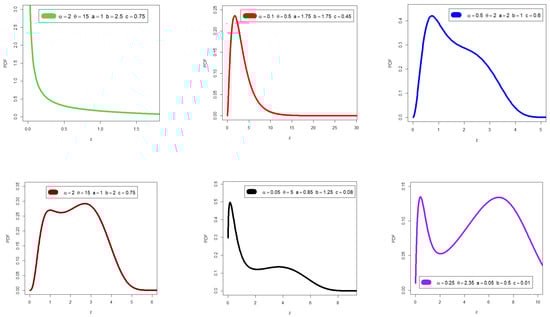
Figure 1.
PDF graphs for some selected parameters values.
Based on Figure 1, it can be seen that the PDF of the new model can be “right skewed heavy tail”, “right skewed heavy tail with one peak”, “right skewed”, and have bimodal density with different shapes. The hazard rate function (HRF) for the GOLLBrXII model can be obtained from . This paper focuses on several estimation methods.
The rest of the paper is organized as follows: The literature review is given in Section 2. Section 3 presents some new properties. The main risk indicators are given in Section 4. Methods of estimation are provided in Section 5. Section 6 presents simulation studies for comparing methods. Section 7 offers data analysis for comparing classical methods and data analysis for comparing models. Risk analysis under insurance claims data utilizing different estimation methods is provided in Section 8. Finally, Section 9 presents some concluding remarks and discussions.
2. Literature Review and Motivation
In this section, a comprehensive literature review is provided to help readers to develop an overall idea about the history of the research problem. This section will include several basic aspects, including those related to the new probability distribution, and others related to applications, including those related to the treatment of actuarial risks and how to evaluate and analyze them.
The BrXII distribution, often known as the Burr distribution, is a continuous probability distribution for a non-negative random variable (NNRV) used in probability theory, statistics, and econometrics; it is one of several alternative distributions referred to as the generalized Burr XII distribution, exponentiated Burr distribution, among others (see Burr [4], Burr [5], Burr [6], Burr and Cislak [7], and Rodriguez [8]). The BrXII distribution has attracted the attention of many researchers in the last two decades, so it has been used in many mathematical and statistical modeling operations, and many researchers have made many generalizations to it, including: the beta BrXII (B BrXII) model was proposed and investigated by Paranaíba et al. [12]. The Kumaraswamy BrXII (KumBrXII) model was put forward and researched by Paranaíba et al. [13]. Yousof et al. [14] created a regression model based on a new family of Burr-Hatke G (BH-G) models. Validation of the BrXII inverse Rayleigh model was conducted by Goual and Yousof [15]. A novel two-parameter BrXII distribution with some copulas, properties, different methods, and modeling acute bone cancer dataset was proposed by Mansour et al. [16]. Elsayed and Yousof [17] developed the generalized Poisson Burr XII (GP BrXII) distribution with four applications by extending the BrXII model. The double BrXII model with censored and uncensored distributional validation utilizing a novel Rao-Robson-Nikulin test was introduced by Ibrahim et al. [18]. Finally, a Bagdonavicius-Nikulin goodness-of-fit test was performed for the compound Topp Leone BrXII model by Khalil et al. [19], among others.
In the actuarial analysis, many works have employed the standard Pareto and standard lognormal distributions to model insurance payments data, and more specifically, massive insurance claim payment data. The extended Pareto has been employed by several academics, including Resnick [20] and Beirlant et al. [21]. The standard Pareto model does not provide a satisfactory match for many actuarial applications when the frequency distributions are hump-shaped because of its monotonically declining density type. In these situations, the standard lognormal is routinely employed to model these datasets, but the lognormal is not suitable for some cases and the Pareto model encompassing more claim payments data. It is clear that left-skewed payment data cannot be explained by the lognormal distribution or the Pareto distribution. To address this flaw in the outdated conventional models, we provide the GOLLBrXII distribution for the negative-skewed insurance claim payments datasets.
In the statistical and actuarial literature, there is a dearth of works that have used probability distributions in the field of processing and analyzing actuarial risks. We mention some of these works, especially the recent ones; for example, see Figueiredo et al. [3], Shrahili et al. [22], and Mohamed et al. ([23,24]). Hence, this important aspect of actuarial science requires a lot of effort to employ probability distributions in the field of actuarial science and to treat, evaluate, and forecast risks.
Although there are numerous established methods for estimation and statistical inference in the statistical literature, we concentrate on the four methods listed above due to their widespread use, effectiveness, and suitability, particularly when combined with the Burr distribution and any derived extensions. These four methods have attracted the attention of many researchers in the last decade. Researchers have used them in statistical modeling and applications in real data. For more details, see Mansour et al. [16] and Ibrahim et al. [18]. We do not mean to imply that these methods do not have failures, or that they do not have defects, but, in any case, we have made every effort to choose the most famous and classic methods with capabilities that are characterized by efficiency and statistical consistency.
3. Properties
3.1. Moment and Asymptotic
Let , the theoretical asymptotic results for the CDF, PDF, and HRF as are given by
and
The theoretical asymptotic results of CDF, PDF, and HRF as are given by
and
The PDF can be rewritten following Cordeiro et al. [11] as
where
and is the PDF of the BrXII model with parameters , and . By integrating (6), the CDF of the GOLLBrXII model is
where is the CDF of the BrXII model with , and . Let be a RV having the BrXII distribution (2) with parameters , and . For , the ordinary and incomplete moments of are, respectively, given by
where and are the beta and the incomplete beta functions of the second type, respectively.
The ordinary moment of is given by Then,
Setting in (8), we obtain the mean of as follows
Furthermore, the can derived as
The variance () can then be obtained from the well-known relationship as
The proportions of the skew coefficient, kurtosis coefficient, failure rate function, and variation in the PDF and failure rate functions all have an impact on how flexible the new distribution is. Additionally, the utility and implementation of the probability distribution in statistical modelling are essential in this context. When we looked at the novel PDF, we found that it was, among other things, highly flexible. This inspired us to critically examine this probability distribution. Using the well-known formulas, the metrics of skewness and kurtosis can be calculated from the standard moments. The effects of the parameters , and on the mean (), variance, skewness, and kurtosis for given values are displayed in Table 2. For Table 2, we note that the GOLLBrXII density can only be right skewed, the kurtosis of the GOLLBrXII model can be more than 3 or less than 3; the parameter has minimal effect on the kurtosis. However, all other parameters have an obvious effect on the kurtosis, the mean of the new model decreases as , and increase and the mean of the new model increases as increases. The moment generated function (MGF) for the GOLLBrXII can be derived due to the expression of Guerra et al. [25], which is calculated as a double infinite sum of incomplete gamma functions.
Table 2.
Numerical analysis for the expected value, the variance, the skewness, the kurtosis under some selected parameter values.
3.2. Incomplete Moments (ICM)
The ICM, say , of the GOLLBrXII distribution can be derived from . From Equation (7), we have
Then,
3.3. Residual and Reversed Residual Life Functions
The moment of the residual life (RSL) is denoted by The moment of the residual life of is given by Then, we can write
The moment reversed residual life (RVRL), . Then, the is defined by
The moment of the RVRL of the RV can then be expressed as
The function = E is called the mean residual lifetime (MRSL) of or its distribution, and is also known as the mean excess loss and the complete expectation of life in insurance. It defines the mean lifetime left for an item of age , or it is the conditional expectation of the residual lifetime of a device at time , given that the device has survived to time . Whereas the failure rate function at provides information on a RV regarding a small interval after , the MRSL function at x considers information regarding the whole remaining interval (,) and satisfies
4. Main Risk Indicators
Actuaries use probability distributions to model and quantify the likelihood of different outcomes and to determine the expected values of future losses. A probability distribution is a function that describes the likelihood of different outcomes for a RV. Actuaries use various types of probability distributions, such as normal, Poisson, exponential, and log-normal, to model different types of risks, such as mortality, morbidity, and property damage. The choice of distribution depends on the nature of the risk being modeled and the data available to support the modeling. Actuaries use probability distributions to calculate the expected values of future losses, which can be used to set insurance premiums, design insurance products, and evaluate investment strategies. Actuaries also use simulation techniques to test their models and to evaluate the impact of various scenarios on the financial outcomes of insurance policies and investments. In this section, we will review a group of important actuarial indicators that are commonly used in evaluating actuarial risks and analyzing the maximum expected losses from the point of view of insurance and reinsurance companies. The new probability distribution is also added according to these actuarial indicators.
4.1. VRk Indicator
Definition 1.
Let denote a loss random variable (LRV). The VRk of at the level, say VRk or , is the quantile (or percentile) of the distribution of .
Then, based on Definition 1, we can simply write for the GOLLBrXII distribution.
where refers to the quantile function of the new model.
4.2. TVRk Risk Indicator
Definition 2.
Let denote a LRV. The TVRk of at the confidence level is the expected loss given that the loss exceeds the of the distribution of , namely
where refers to the significant level.
Then,
Thus, the quantity is an average of all values above the confidence level , which provides more information about the tail of the GOLLBrXII distribution. Finally, can also be obtained from
where is the mean excess loss function (MELF) evaluated at the quantile. Therefore, is larger than its corresponding by the amount of average excess of all losses that exceed the MELF value. In the insurance literature, has been independently developed and it is also called the conditional tail expectation. It is also called the tail conditional expectation (TCE) or expected shortfall (ES) (Tasche [26]; Acerbi and Tasche [27]).
4.3. TV Risk Indicator
Definition 3.
Let denote a LRV. The TV risk indicator (TV ()) can be expressed as
Then, for the GOLLBrXII model, we have
4.4. TMV Risk Indicator
Definition 4.
Let denote a LRV. Then, the TMV can be derived as
Then, for any LRV, , , for the and for the .
5. Methods of Estimation
5.1. Maximum Likelihood Method
A statistical technique called maximum likelihood estimation (MLE) is used to determine the unknown parameters of a certain probabilistic model. To accomplish this, a likelihood function is optimized to increase the probability of the observed data under the presumptive statistical model. The parameter space position, where the likelihood function is optimum, is known as the estimate of the maximum likelihood. Maximum likelihood’s fundamental reasoning is simple and adaptable, and as a result, the technique has taken the lead among statistical inference approaches. The derivative test can be used to identify maxima if the likelihood function is differentiable. The ordinary least squares estimator for a linear regression model, for example, maximizes the likelihood when all observed outcomes are assumed to have normal distributions with the same variance. In certain circumstances, the first-order requirements of the likelihood function may be analytically solved. The log-likelihood function is given by
The function can be optimized by the numerical methods via many programs such as SAS and R, among others. The components of the score vector are
In this regard, we do not intend to develop more algebraic derivations or predictive results in order to focus more on practical aspects and numerical results, especially with regard to simulation results and the results of actuarial risk analysis. However, if you request these derivations, we will provide them.
5.2. The Ordinary Least Square Method
Ordinary least squares estimation (ORLSE), also known as linear least squares, is a statistical technique for figuring out the unknown variables in the model linear regression. In the ORLSE, the sum of squared (SS) vertical distances between the dataset’s observed responses and those anticipated by the linear approximation are minimized using this technique. Particularly when there is just one regressor on the right-hand side, the resultant estimate may be represented using a straightforward formula. The ORLSE is the maximum likelihood estimator when the extra supposition that the errors are normally distributed is held. There are various applications for ORLSE, including econometrics in economics and control theory and signal processing in electrical engineering. Suppose , which refers to the CDF of the GOLLBrXII model, and if be the ordered random sample. The ORLSEs are obtained upon minimizing the following function
where The ORLSEs are obtained via solving the following nonlinear equations that can be easily derived and solved.
5.3. The Weighted Least Square Method
The estimators of the weighted least squares estimation (WLSE) method are unbiased and their estimators have the least variance, unlike many other characteristics that prompted us to use this method. The method has proven its importance and high ability in statistical modeling operations, but in this paper, we employ the method in actuarial risk assessments, and the statistical literature is very scarce in this direction. The WLSE are obtained by minimizing the given form of the equation with respect to the parameters.
where
5.4. Method of Cramer-Von-Mises
The Cramer-Von-Mises estimation (CVME) of the parameters , and are obtained by minimizing
where . Then, the CVME of the parameters are obtained by solving its non-linear equation.
6. Simulation Studies for Comparing Methods
In this section, Monte-Carlo simulation experiments are performed to investigate the effectiveness of the different estimators of the GOLLBrXII distribution’s unknown parameters. The mean squared errors of the various estimators proposed in the preceding section are used to assess their performance (MSEs). We generate 10,000 samples of the GOLLBrXII distribution, where and by choosing initial values as presented in Table 3. The average (AVs) and corresponding values (MSEs) of the estimates for the MLE, ORLSE, WLSE, and CVME methods are reported in Table 4, Table 5, Table 6, Table 7 and Table 8. From Table 4, Table 5, Table 6, Table 7 and Table 8, we can observe that all the estimates for all the selected methods show consistency; i.e., the MSEs decrease as increases. The following results can be highlighted:
Table 3.
Two scenarios for simulations.
Table 4.
MSEs for = 20.
Table 5.
MSEs for = 50.
Table 6.
MSEs for = 100.
Table 7.
MSEs for = 200.
Table 8.
MSEs for = 300.
- For the MLE method (initial values I): MSEs for started with 0.15864 | and ended with 0.00724 | For the MLE method (initial values I): MSEs for started with 0.07010 | and ended with 0.00134 | For the MLE method (initial values I): MSEs for started with 0.05180 | and ended with 0.00018 | For the MLE method (initial values I): MSEs for started with 0.25890 | and ended with 0.01435 | The same comments can be easily addressed.
- The MLE method is the best method in general with the smallest MSEs; then CVMEs, then ORLSEs, and then WLSEs for the most sample sizes.
7. Real-Life Data Analysis and Related Comparisons
In this section, we provide two subsections; the first for comparing the methods with two examples, and the second for comparing models with two applications.
7.1. Data Analysis for Comparing Classical Methods
Model selection is the process of choosing the best model from a pool of candidates based on the performance criteria. This could involve choosing a statistical method from a list of potential models after considering data in the context of learning. In the simplest scenarios, an existing set of data is taken into account. However, the work could also entail planning trials so that the information gathered is useful for the challenge of model choice. The simplest model is still most likely to be the best option when there are several candidate models with comparable explanatory or predictive potential. In the previous section, we compared different estimation methods through reliability data and through a comprehensive simulation study. In this section, we compare the estimation methods, but through two sets of real data. Although we presented the results of the simulation study with some useful comments, the goal of the simulation differs from the goal of applications to real data. In the simulation, we mainly aim to evaluate the behavior of the estimators of the methods with increasing sample size. As for applications, we aim to provide a real comparison between methods in order to determine the best and worst methods in statistical modeling operations. In this direction, we analyzed two sets of engineering and medical data.
Example 1.
Dataset I can be called the breaking stress reliability data. This data consists of 100 observations of the breaking stress of carbon fibers (in Gba) (see Nichols and Padgett [28]). We consider the Cramér-Von Mises , the Anderson-Darling statistics, Kolmogorov Smirnov (KST) and its corresponding p-value.
Table 9 presents the values of estimators of , , , and where and the and statistics for the classical mothods. Figure 2 presents the Kaplan-Meier survival graphs for the breaking stress data.
Table 9.
The values of estimators for all estimation methods, and , KST, and p-value for the breaking stress.
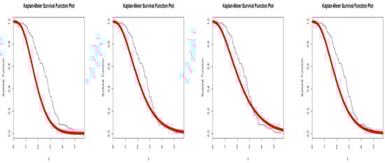
Figure 2.
Kaplan-Meier survival graphs (MLE (first panel), ORLSE (second panel), WLSE (third panel), CVME (fourth panel)) for the breaking stress data.
Based on Table 9, the CVM is recommended to be the best method because it showed the best possible results among all the classical estimation methods used in the estimation with KST = 0.08905 and p-value = 0.40594. At the same time, we do not deny that the remaining methods (ORLSE and WLSE) give acceptable results, which are very close to ML and CVM. For this very reason, the graphs in Figure 2 may not show a significant difference between the four methods used for estimation.
Example 2.
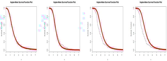
Dataset II is survival times (in days) of 72 guinea pigs infected with virulent tubercle bacilli (see Bjerkedal [29]). Table 10 gives the values of estimators of , , , and where and the and statistics for the classical mothods. Figure 3 presents the Kaplan-Meier survival graphs for the breaking stress data. Based on Table 10, the CVME is recommended to be the best method because it showed the best possible results among all the classical estimation methods used in the estimation with KST = 0.06777 and p-value = 0.89555. At the same time, we do not deny that the remaining methods (ORLSE and WLSE) give acceptable results, which are very close to MLE and CVME. Perhaps for this very reason, the graphs in Figure 3 may not show a significant difference between the four methods used for estimation.
Table 10.
The values of estimators for all estimation methods, and , KST, and p-value for the survival times.
Figure 3.
Kaplan-Meier survival graphs (MLE (first panel), ORLSE (second panel), WLSE (third panel), CVME (fourth panel)) for the survival times data.
7.2. Data Analysis for Comparing Classical Methods
We provide two applications to illustrate the importance, potentiality, and flexibility of the GOLLBrXII model using the same datasets in Section 6. We compare the GOLLBrXII distribution with BrXII, Marshall-Olkin BrXII (MOBrXII), Topp Leone BrXII (T-LBrXII), five-parameters beta-BrXII (5PBBrXII), zografos-Balakrishnan BrXII (Z-BBrXII), Beta BrXII (B BrXII), Beta exponentiated BrXII (BEBrXII), five-parameters Kumaraswamy-BrXII (5PKwBrXII), and Kumaraswamy-BrXII (KwBrXII) distributions. For more details regarding these competitive models, see Elsayed and Yousof [17] and Ibrahim et al. [18].
The total time in test (TTT) graphs for all real-life datasets are presented in Figure 4, and they indicate that the empirical HRFs of the two datasets are monotonically increasing (see Figure 4). The Akaike information (AIC), Bayesian information (BIC), Hannan-Quinn information (HQIC), consistent Akaike information (CAIC), and goodness-of-fit statistics are considered for comparing models. The MLEs, standard errors (SEs), and 95% confidence intervals (CI) for the first data set are provided in Table 11. The AIC, BIC, CAIC, and HQIC for datasets I are shown in Table 12. The MLEs, standard errors (SEs), and 95% confidence intervals (CI) for the second data set are provided in Table 13. The AIC, BIC, CAIC, and HQIC for datasets II are shown in Table 14. Based on the data in Table 12 and Table 14, the GOLLBrXII model offers the best fits in the two applications when compared to other BrXII models, with the least values for BIC, AIC, CAIC, and HQIC.
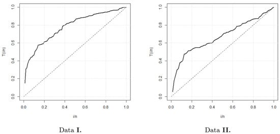
Figure 4.
TTT graphs.
Table 11.
MLEs, SEs, and CI for the breaking stress data.
Table 12.
AIC, BIC, CAIC, and HQIC for breaking stress.
Table 13.
MLEs, SEs, and CI for the survival data.
Table 14.
AIC, BIC, CAIC, and HQIC for survial data.
The predicted PDF graphs for the two real sets of data are shown in Figure 5. The predicted CDF graphs for the two real datasets are displayed in Figure 6. The calculated HRF charts for the two genuine datasets are shown in Figure 7. Figure 8 lists the P-P graphs for the two real datasets, respectively. Figure 9 provides the Kaplan-Meier survival graphs for the two real datasets, respectively. We can see that the revised model provides a satisfactory fit from Figure 5, Figure 6, Figure 7, Figure 8 and Figure 9 (estimated PDFs, estimated CDFs, estimated HRFs, P-P graphs, and Kaplan-Meier survival graphs). Given that the comparisons were carried out using four distinct statistical standards, Table 12 and Table 14 reveal that the new distribution (via two sets of data) has demonstrated its superiority over a significant number of other distributions by other authors.
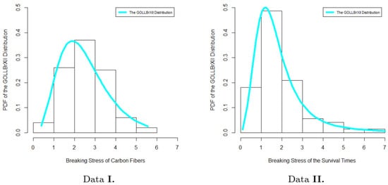
Figure 5.
Estimated PDFs for the two real datasets.
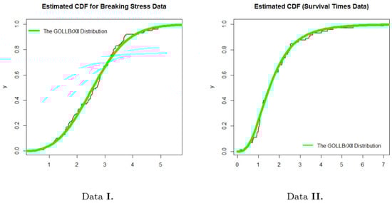
Figure 6.
Estimated CDFs for the two real datasets.
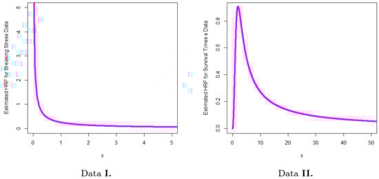
Figure 7.
Estimated HRFs for the two real datasets.
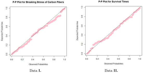
Figure 8.
P-P graphs for the two real datasets.
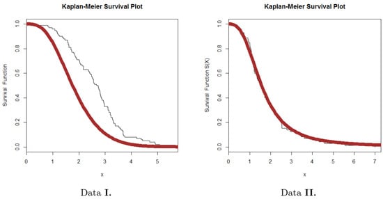
Figure 9.
Kaplan-Meier survival graphs for the two real datasets.
8. Risk Analysis under Insurance Claims Data Utilizing Different Estimation Methods
Actuaries have recently used continuous distributions, especially ones with broad tails, to reflect actual insurance data. Engineering, risk management, dependability, and the actuarial sciences are just a few of the application areas where real data has been simulated using continuous heavy-tailed probability distributions. The skewness of insurance datasets can be either left, right, or right with exceptionally large tails. In this paper, we show how the flexible continuous heavy-tailed GOLLBrXII distribution can be used to represent left-skewed insurance claims data.
Utilizing insurance claims data is challenging despite its huge value. The largest issue is evaluating its quality and counting the number of incomplete or missing observations (see Stein et al. [30] and Lane [31]). For further details, see Ibragimov and Prokhorov [32], Cooray and Ananda [33], Hogg and Klugman [1], and Lane [31]. Real datasets for insurance payments are commonly heavy or right tailed, and they are generally positive. In this section, using a U.K. Motor Non-Comprehensive account as a concrete example, we look at the insurance claims payment triangle. Convenience led us to pick the genesis era from 2007 to 2013 (see Charpentier [34], Shrahili et al. [22], Mohamed et al. [23,24]).
The claims data are presented in the insurance claims payment data frame in the same way that a database would typically store it. The first column contains the development year, the incremental payments, and the origin year, which spans from 2007 to 2013. It is vital to remember that a probability-based distribution was initially used to examine these data on insurance claims. The insurance premium is the sum of money an individual or business pays to purchase an insurance policy. For the coverage of life, an automobile, a house, and health insurance, premiums are paid. Once the premium is earned, the insurance company is paid. It also entails a liability because the insurer is obligated to provide coverage for any claims brought up in relation to the policy. The policy may be cancelled if either the individual or the business fails to pay the premium. In this work, we focus our work on the insurance claims side, which is what was from the data. Perhaps we will find the opportunity in the future to carry out a balanced study examining the claims and the premiums.
We start by examining the data on insurance claims statistics, but this time for data on insurance claims. It is possible to quantitatively, visually, or by combining the two, evaluate real-world data. Initial fits of theoretical distributions such as the normal, exponential, logistic, beta, uniform, lognormal, and Weibull are assessed using the numerical technique (see Table 11), as well as other several graphical/statistical tools, such as the skewness-kurtosis graph (or the Cullen-Frey graph) (see Figure 10).
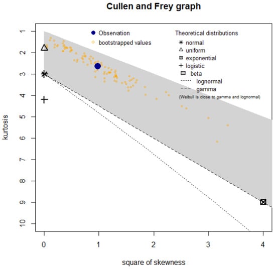
Figure 10.
Cullen-Frey graph for claims payment data.
The nonparametric density estimation (NKDE) method for examining the initial shape of the insurance claims density, the Q-Q graph for examining the “normality” of the current data, the TTT graph for examining the initial shape of the HRF, and the “box graph” for identifying the extreme claims are just a few of the additional graphical methods that are taken into consideration (see Figure 11, bottom right graph). The top left graph of Figure 11 shows the initial density as an asymmetric function with a left tail. No extreme values are shown from Figure 11 (bottom right graph).
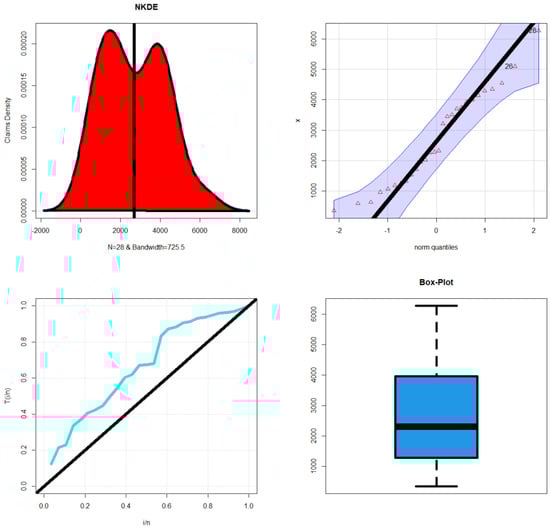
Figure 11.
NKDE graph (top left graph), Q-Q graph(top right graph), TTT graph (bottom left graph), and box graph (bottom right graph) for insurance claims data.
In addition, the bottom left graph of Figure 11 shows that the HRF for the models that account for the observed data should be “monotonically increasing”. It is important to note that there are numerous risk indicators that can be used and employed in the assessment and analysis of actuarial risks. Additionally, there is room for the introduction of new risk indicators that might perform better in some theoretical and practical respects than the established ones. We think that there is still a lot of work to be done in the area of actuarial statistical programming in order to develop more specialized actuarial packages that might make the work of insurance and reinsurance businesses easier.
The first row in Figure 12 shows scattergrams for the data on insurance claims, while the second row shows the autocorrelation function (ACF) and partial autocorrelation function (partial ACF). We provide the ACF that may be used. Figure 12 illustrates the distribution of hills and valleys on the surface with Lag = k = 1 in more detail (bottom left). Theoretical partial ACF with Lag = k = 1 is shown in Figure 12 (the bottom right panel). According to the bottom right corner of Figure 12, the initial lag value is statistically significant; however, none of the other partial autocorrelations for any other delays are. In order to potentially fit these data, an autoregressive (AR(1)) model is suggested.
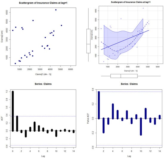
Figure 12.
Scattergrams, ACF, and practical ACF for the the insurance claims data.
The initial NKDE is an asymmetric function with a left tail, as shown in the top left panel of Figure 12. On the other hand, the left tail form is present in the novel model’s density. As a result, it is advised to use the GOLLBrXII model to model the payouts for insurance claims. We present an application for risk assessment and analysis under VRk, TVRk, TV, and TMV measures for the insurance claims data. The risk analysis is conducted for some confidence levels
The five measures are analyzed and then estimated for the GOLLBrXII and Burr XII models. The Burr XII model is the better baseline model for this application. Table 15 summarizes the estimated parameters for KRKIs for the GOLLBrXII and Burr XII models, Table 16 reports the KRKIs for the GOLLBrXII model, and Table 17 reports the KRKIs for the Burr XII model.
Table 15.
Estimated parameters for KRKIs for GOLLBrXII and Burr XII models.
Table 16.
KRKIs under the insurance claims data for the GOLLBrXII model.
Table 17.
KRKIs under the insurance claims data for the Burr XII model.
Table 18 provides the VRk range under the new model and the baseline model for all values. Based on Table 18, the new model is better for all values. Insurance companies can rely on the new distribution in determining the minimum and maximum limits for the volume of insurance claims. This reluctance of claims, which was estimated in the light of historical data, could achieve some safety for insurance companies in avoiding the risks of an inability to pay insurance claims.
Table 18.
VRk range under the new model and the baseline model for all values.
- I.
- Under the MLEs: For the GOLLBrXII model, the quantity VRk ranges from 3313.4 to 17414.62; however, for the Burr XII model, the quantity VRk ranges from 3398.65 to 7369.73.
- II.
- For the GOLLBrXII model, the quantity TVRk ranges from 6610.75 to 32,345.5; however, for the Burr XII model, the quantity TVRk ranges from 4701.5 to 8285.6.
- III.
- For the GOLLBrXII model, the quantity TV ranges from 125,688,493.43 to 2,884,628,282.96; however, for the Burr XII model, the quantity TV ranges from 1,309,732.22 to 776,459.57.
- IV.
- For the GOLLBrXII model, the quantity TMV ranges from 62,850,857.47 to 1,442,346,487.03; however, for the Burr XII model, the quantity TMV ranges from 659,567.64 to 396,515.42.
- V.
- For the GOLLBrXII model, the quantity MELF ranges from 3297.36 to 14,930.9; however, for the Burr XII model, the quantity MELF ranges from 1302.88 to 915.91. However, the same comments can be addressed.
9. Concluding Remarks
The probability-based distributions could provide a reasonable explanation for the exposure to risk. Most often, one number, or at least a small collection of numbers, are used to indicate the level of risk exposure. We examine the actuarial risks using the five previously stated indicators in order to study and evaluate the risks that insurance firms may face in relation to the payment of insurance claims. Four estimation methods are used to calculate these five fundamental indicators. A novel distribution, known as the generalized odd log-logistic Burr type XII, is given and studied as a consequence, keeping this main goal in mind. Through Monte Carlo simulations, the performance of each estimating method is examined. For comparing traditional methodologies, two actual data applications are shown. For comparing the new model with other competing models and demonstrating the significance of the suggested model using the maximum likelihood technique, two actual data applications are offered. The four approaches indicated above and five actuarial indicators based on bimodal insurance claims payment data are used to analyze and evaluate the actuarial risks. The following results can also be shown for most values of :
- I.
- for the GOLLBrXII model VRk for the Burr XII model
- II.
- for the GOLLBrXII model TVRk for the Burr XII model.
- III.
- for the GOLLBrXII model TV for the Burr XII model.
- IV.
- for the GOLLBrXII model TMV for the Burr XII model.
- V.
- VI.
- VII.
- VIII.
- IX.
The generalized odd log-logistic Burr XII model can also be employed for the stress-strength models and multicomponent stress-strength models. It is worth noting that there are many risk indicators that can be used and employed in the evaluation and analysis of actuarial risks, and the door is open to presenting more new risk indicators that may outperform the well-known indicators in some theoretical and applied aspects. We believe that the field of actuarial statistical programming still needs a lot of efforts to provide more specialized actuarial packages that may facilitate the work of insurance and reinsurance companies.
Author Contributions
H.M.Y.: review and editing, data duration, software, validation, writing the original draft preparation, conceptualization; S.I.A.: validation, data duration, conceptualization, writing the original draft preparation, data curation; Y.T.: methodology, data duration, conceptualization, software; W.E.: validation, writing the original draft preparation, conceptualization, data curation, formal analysis, data duration, software; M.M.A.: review and editing, conceptualization, data duration, supervision; M.I.: review and editing, software, data duration, validation, writing the original draft preparation, conceptualization; S.L.A.: review and editing, data duration, software, validation, writing the original draft preparation, conceptualization. All authors have read and agreed to the published version of the manuscript.
Funding
The study was funded by Researchers Supporting Project number (RSP2023R488), King Saud University, Riyadh, Saudi Arabia.
Data Availability Statement
The dataset can be provided upon requested.
Acknowledgments
The study was funded by Researchers Supporting Project number (RSP2023R488), King Saud University, Riyadh, Saudi Arabia.
Conflicts of Interest
The authors declare no conflict of interest.
References
- Hogg, R.V.; Klugman, S.A. Loss Distributions; John Wiley & Sons, Inc.: New York, NY, USA, 1984. [Google Scholar]
- Artzner, P. Application of coherent risk measures to capital requirements in insurance. N. Am. Actuar. J. 1999, 3, 11–25. [Google Scholar] [CrossRef]
- Figueiredo, F.; Gomes, M.I.; Henriques-Rodrigues, L. Value-at-risk estimation and the PORT mean-of-order-p methodology. Revstat 2017, 15, 187–204. [Google Scholar]
- Burr, I.W. Cumulative frequency functions. Ann. Math. Stat. 1942, 13, 215–232. [Google Scholar] [CrossRef]
- Burr, I.W. On a general system of distributions, III. The simple range. J. Am. Stat. Assoc. 1968, 63, 636–643. [Google Scholar]
- Burr, I.W. Parameters for a general system of distributions to match a grid of α 3 and α 4. Commun. Stat. 1973, 2, 1–21. [Google Scholar] [CrossRef]
- Burr, I.W.; Cislak, P.J. On a general system of distributions: I. Its curve-shaped characteristics; II. The sample median. J. Am. Stat. Assoc. 1968, 63, 627–635. [Google Scholar]
- Rodriguez, R.N. A guide to the Burr type XII distributions. Biometrika 1977, 64, 129–134. [Google Scholar] [CrossRef]
- Tadikamalla, P.R. A look at the Burr and related distributions. Int. Stat. Rev. 1980, 48, 337–344. [Google Scholar] [CrossRef]
- Gupta, R.C.; Gupta, R.D. Proportional reversed hazard rate model and its applications. J. Statist. Plan. Inference 2007, 137, 3525–3536. [Google Scholar] [CrossRef]
- Cordeiro, G.M.; Alizadeh, M.; Ozel, G.; Hosseini, B.; Ortega, E.M.M.; Altun, E. The generalized odd log-logistic family of distributions: Properties, regression models and applications. J. Stat. Comput. Simul. 2017, 87, 908–932. [Google Scholar] [CrossRef]
- Paranaíba, P.F.; Ortega, E.M.; Cordeiro, G.M.; Pescim, R.R. The beta Burr XII distribution with application to lifetime data. Comput. Stat. Data Anal. 2011, 55, 1118–1136. [Google Scholar] [CrossRef]
- Paranaíba, P.F.; Ortega, E.M.; Cordeiro, G.M.; Pascoa, M.A.D. The Kumaraswamy Burr XII distribution: Theory and practice. J. Stat. Comput. Simul. 2013, 83, 2117–2143. [Google Scholar] [CrossRef]
- Yousof, H.M.; Altun, E.; Ramires, T.G.; Alizadeh, M.; Rasekhi, M. A new family of distributions with properties, regression models and applications. J. Stat. Manag. Syst. 2018, 21, 163–188. [Google Scholar] [CrossRef]
- Goual, H.; Yousof, H.M. Validation of Burr XII inverse Rayleigh model via a modified chi-squared goodness-of-fit test. J. Appl. Stat. 2020, 47, 393–423. [Google Scholar] [CrossRef] [PubMed]
- Mansour, M.; Yousof, H.M.; Shehata, W.A.M.; Ibrahim, M. A new two parameter Burr XII distribution: Properties, copula, different estimation methods and modeling acute bone cancer data. J. Nonlinear Sci. Appl. 2020, 13, 223–238. [Google Scholar] [CrossRef]
- Elsayed, H.A.H.; Yousof, H.M. Extended Poisson Generalized Burr XII Distribution. J. Appl. Probab. Stat. 2021, 16, 1–30. [Google Scholar]
- Ibrahim, M.; Ali, M.M.; Goual, H.; Yousof, H. The Double Burr Type XII Model: Censored and Uncensored Validation Using a New Nikulin-Rao-Robson Goodness-of-Fit Test with Bayesian and Non-Bayesian Estimation Methods. Pak. J. Stat. Oper. Res. 2022, 18, 901–927. [Google Scholar] [CrossRef]
- Khalil, M.G.; Yousof, H.M.; Aidi, K.; Ali, M.M.; Butt, N.S.; Ibrahim, M. Modified Bagdonavicius-Nikulin Goodness-of-fit Test Statistic for the Compound Topp Leone Burr XII Model with Various Censored Applications. Stat. Optim. Inf. Comput. 2023. [Google Scholar]
- Resnick, S.I. Discussion of the Danish data on large fire insurance losses. ASTIN Bull. 1997, 27, 139–151. [Google Scholar] [CrossRef]
- Beirlant, J.; Joossens, E.; Segers, J. Generalized Pareto fit to the society of actuaries large claims database. N. Am. Actuar. J. 2004, 8, 108–111. [Google Scholar] [CrossRef]
- Shrahili, M.; Elbatal, I.; Yousof, H.M. Asymmetric Density for Risk Claim-Size Data: Prediction and Bimodal Data Applications. Symmetry 2021, 13, 2357. [Google Scholar] [CrossRef]
- Mohamed, H.S.; Ali, M.M.; Yousof, H.M. The Lindley Gompertz Model for Estimating the Survival Rates: Properties and Applications in Insurance. Ann. Data Sci. 2022, 1–19. [Google Scholar] [CrossRef]
- Mohamed, H.S.; Cordeiro, G.M.; Minkah, R.; Yousof, H.M.; Ibrahim, M. A size-of-loss model for the negatively skewed insurance claims data: Applications, risk analysis using different methods and statistical forecasting. J. Appl. Stat. 2022, 1–22. [Google Scholar] [CrossRef]
- Guerra, R.R.; Peña-Ramirez, F.A.; Peña-Ramirez, M.R.; Cordeiro, G.M. A note on the density expansion and generating function of the beta Burr XII. Math. Methods Appl. Sci. 2020, 43, 1817–1824. [Google Scholar] [CrossRef]
- Tasche, D. Expected Shortfall and Beyond. J. Bank. Financ. 2002, 26, 1519–1533. [Google Scholar] [CrossRef]
- Acerbi, C.; Tasche, D. On the coherence of expected shortfall. J. Bank. Financ. 2002, 26, 1487–1503. [Google Scholar] [CrossRef]
- Nichols, M.D.; Padgett, W.J. A bootstrap control chart for Weibull percentiles. Qual. Reliab. Eng. Int. 2006, 22, 141–151. [Google Scholar] [CrossRef]
- Bjerkedal, T. Acquisition of resistance in Guinea pigs infected with different doses of virulent tubercle bacilli. Am. J. Hyg. 1960, 72, 130–148. [Google Scholar]
- Stein, J.D.; Lum, F.; Lee, P.P.; Rich, W.L., III; Coleman, A.L. Use of health care claims data to study patients with ophthalmologic conditions. Ophthalmology 2014, 121, 1134–1141. [Google Scholar] [CrossRef]
- Lane, M.N. Pricing risk transfer transactions 1. ASTIN Bull. J. IAA 2000, 30, 259–293. [Google Scholar] [CrossRef]
- Ibragimov, R.; Prokhorov, A. Heavy Tails and Copulas: Topics in Dependence Modelling in Economics and Finance; World Scientific: Singapore, 2017. [Google Scholar]
- Cooray, K.; Ananda, M.M. Modeling actuarial data with a composite lognormal-Pareto model. Scand. Actuar. J. 2005, 2005, 321–334. [Google Scholar] [CrossRef]
- Charpentier, A. Computational Actuarial Science with R; CRC press: Boca Raton, FL, USA, 2014. [Google Scholar]


Disclaimer/Publisher’s Note: The statements, opinions and data contained in all publications are solely those of the individual author(s) and contributor(s) and not of MDPI and/or the editor(s). MDPI and/or the editor(s) disclaim responsibility for any injury to people or property resulting from any ideas, methods, instructions or products referred to in the content. |
© 2023 by the authors. Licensee MDPI, Basel, Switzerland. This article is an open access article distributed under the terms and conditions of the Creative Commons Attribution (CC BY) license (https://creativecommons.org/licenses/by/4.0/).