1. Introduction
Pairs trading is a statistical arbitrage strategy that emerged from a Morgan Stanley quantitative group from in the 1980s. Investors choose a pair of highly-correlated securities, buy the relatively under-priced security, and sell the relatively over-priced security simultaneously, with the expectation of making a profit from the price spread regression. In this paper, we discuss the dynamic mean-variance (MV) problem for pairs trading in the Scott model, a fast-mean-reverting volatility model.
The cointegration approach is popular in pairs trading and was proposed by Vidyamurthy [
1]. Vidyamurthy assessed the co-movement of securities through conintegration testing and designed a trading rule based on a simple nonparametric threshold. Lin et al. [
2] studied the optimal trading threshold problem by introducing a minimum profit condition for a conintegrated pair of stocks. In a recent work by Yan et al. [
3], they discussed pairs trading under a delayed cointegration model. In the cointegration framework, it is very important to model price spread. Elliott et al. [
4] described spread using a mean-reverting Gaussian Markov chain model and developed an analytical framework for pairs trading strategies. Bertram [
5] developed a statistical arbitrage model for the spread of two log price series under the assumption of the OU process. Many authors have viewed the optimal pairs trading problem as a stochastic control problem and have considereded it by maximizing a variety of utility functions. Jurek and Yang [
6] discussed asset allocation strategies between a mean reverting arbitrage opportunity described by an OU process and a risk-free asset and assigned a closed-form, optimal allocation for CRRA utility over a finite time horizon. Suzuki [
7,
8] and Endres and Stübinger [
9] solved an optimal regime switching problem with the constraints of finite transaction times and transaction fees. Liu and Timmermann [
10] derived a closed-form optimal strategy based on the cointegration assumption with the power utility over the terminal wealth. Chiu and Wong [
11] assumed that the log prices of the risky assets satisfy the linear stochastic differential equation with a constant matrix of cointegration coefficients. They considered the time-consistent dynamic mean-variance problem (according to dynamic programming)and provided a closed-form optimal strategy. Recently, Zhu et al. [
12] assumed that price spread follows an OU process and that one of the corresponding securities satisfies the geometric Brownian motion(GBM) model with a constant volatility. They considered the time-consistent mean-variance problem (see Björk et al. [
13]) for pairs trading and provided a closed-form optimal strategy.
However, in all of the models mentioned above, the drift and the volatility of the (log) price processes are all deterministic functions or constants that are unable to capture some of the stochastic volatility characteristics that can be observed in many markets, such as mean reversion effects, see Cont [
14,
15], Teräsvitra and Zhao [
16], and Gatheral et al. [
17] for empirical evidence related to this. Therefore, in this paper, we assume that price spread follows an OU process and that one of the log prices of the securities satisfies a stochastic volatility model (SVM). Additionally, we discuss the dynamic mean-variance problem in the means of Björk et al. [
13]. Because an SVM can describe price dynamics better, it is more likely to develop strategies that can be used to control trading risk more precisely and bring about greater utility. In this paper, we first discuss the optimal strategy for pairs trading under a general SVM by a PDE. Then, we specify a fast mean-reverting stochastic volatility model, the Scott model [
18], and discuss the approximate optimal strategy.
The main contributions of this paper are as follows: First, we provide a semi-closed-form of the optimal strategy under a general SVM based on the solution of a PDE. Second, we provide an closed-form approximation of the optimal strategy under a fast mean-reverting volatility model that captures the mean-reverting property of volatilities by using the asymptotic analysis technique. Our approximate formula can be proven to have sufficient precision and extremely high computational efficiency compared with the traditional finite difference method(FDM), which is of great practical value. Finally, we calibrate the model parameters using securities data from the Chinese stock markets, and demonstrate the effect of our approximated optimal strategy by comparing it with the optimal strategy described in Zhu et al. [
12]. Empirical studies show that the Scott model can produce a more stable strategy by better capturing mean-reverting volatility.
The remainder of this paper is organized as follows: In
Section 2, we describe the model specifications as well as the optimal dynamic MV problem and provide the semi-closed-form optimal strategy based on a PDE. In
Section 3, we provide a closed-form approximation of the optimal strategy for the Scott volatility model. In
Section 4, we validate the trading strategy empirically using Chinese securities market data.
Section 5 concludes the paper.
2. The Dynamic Mean-Variance Problem for a General Stochastic Volatility Modelstochastic volatility models
In this section, we set up the dynamic mean-variance(MV) problem for pairs trading under a general SVM. Since the MV problem is time inconsistent, we discuss the optimal strategy, according to the definition of the equilibrium strategy introduced by [
13] by transforming the dynamic MV problem to a non-cooperative Nash equilibrium game.
Assume that
is a complete probability space and that,
,
and
are Brownian motions with
We assume that is the filtration generated by , and . The conditional expectation and conditional variance with respect to are denoted as and .
We assume that there is a pair of conintegrated securities denoted as P and Q. The price processes of P and Q are denoted by and , and there is a tradable risk-free asset whose price process is denoted by . Furthermore, we also assume that the market is frictionless, i.e., there are no transaction costs and taxes, and that short selling is allowed.
Assume that the dynamic of the price
satisfies the following stochastic volatility model:
where
is a constant. We assume that the spread of the log-prices log-price of
P and
Q satisfies an OU process. Let
be the spread of the log-prices; then log-price, then
satisfies the following SDE:
where
,
, and
are all constants. The dynamic of the risk-free asset
is given by
Remark 1. Since , according to Itô’s formula, one can see that satisfies the following SDE: We denote
as the weights invested in the securities
P and
Q at time
t in a symmetric pairs trading strategy, and the corresponding wealth process
is given by
Substituting (
1) and (
3) into (
4), one can see that
Let
be the discounted money invested in the security
P, which can be viewed as a strategy; then, the discounted wealth process
is given by
Assume that the discounted wealth at time
is
, then
Let
where
, we consider the following dynamic MV problem:
Because of the time-inconsistency of the MV problem (
8), we introduce the optimal strategy according to the definition of equilibrium strategy provided in Björk et al. [
13].
Definition 1. The strategy is called an optimal strategy if for any permutation ,holds for any . We have the following theorem
Theorem 1 (Main result I). Define . The optimal strategy for the dynamic MV problem (8) is given bywhere is a solution to the following equation:where with the terminal condition . Lemma 1. Let be the strategy given in Theorem 1 and be a solution of the Equation (10); then, Proof. Let
. It follows from Itô’s formula that
One can see that
is a martingale; thus,
which implies (
11). □
Proof of Theorem 1. For the given
, let
be any permutation of
. For any strategy
, introduce
Since
is not dependent on the corresponding discounted wealth process
, it follows from (
6) that
Furthermore, it follows from the proof of Lemma 1 and (
6) that
thus
which completes the proof. □
Remark 2. From the proof of Theorem 1, we can see that is the solution of the following HJB equation: Remark 3. It is unlikely that a closed-form solution of the PDE (10) can be achieved without specifying . Therefore, we will consider the Scott model, one of the most widely known mean-reverting stochastic volatility models, and will discuss the approximate solution. 3. Closed-Form Approximation under the Scott Model
In order to capture the fast mean-reverting characteristics of volatility (see Fouque [
19,
20] for empirical studies), we introduce the Scott model, initially proposed by Scott (1987) [
18], which is a well-known mean-reverting volatility model. Under the Scott model, the underlying security price is modeled by:
where
and
. Since
,
,
. Clearly, the volatility is modeled by an OU process. We assume
to ensure the fast mean-reverting property and set
for convenience. According to Theorem 1, the corresponding PDE for the optimal strategy is given by:
where
with the terminal condition
. It is difficult to solve the PDE (
12) explicitly and to achieve a closed-form optimal strategy. Therefore, in this section, we will use the asymptotic analysis technique to find a closed-form approximation of the PDE (
12).
Let
; one can see from (
12) that
satisfies the following PDE:
Let
and
. Since
, it is reasonable to assume that
. We introduce the following operator
where
Then the PDE (
13) can be written in the following form
To provide an approximation for
, we need to introduce
and define the functional
as
for all
h such that
. The following lemma can be found in Fouque [
19].
Lemma 2. The following equationonly has a solution if satisfiesfor each , . 3.1. An Approximation for
Assume that
g is a solution of (
14). We can construct an asymptotic expansion with respect to
for
g as the following
Substituting it into (
14), we obtain
For simplicity, we assume that
,
. Since the operator
only involves partial derivatives with respect to
y, one can see that
Then, Equation (
15) can be simplified into the following form
It is natural to consider the following equations
To make sure the Equation (
17) has a solution, it follows from Lemma 2 that for each
, the right part of (
17) should satisfy the following equation
Since
, if we let
, one can see that
Furthermore, from the definition of
, one can see that
which is a linear function of
x. Assigning the boundary value of
as
, the solution can be directly given by
Similarly, to ensure that Equation (
18) has a solution, we need
With the bound condition
, one can see that
is a solution. Therefore, a natural approximation for
is given by
Thus, we have the following theorem:
Theorem 2 (Main result II). Denote . Let Then, there exists a constant C that is independent of ϵ such that An approximate optimal strategy is given by Remark 4. Compared with the traditional finite difference method(FDM), we can obtain an explicit solution with a significant advantage in computational complexity using the asymptotic analysis technique. In practice, at each decision moment, we only need to calculate the optimal strategy at one specific point , which describes the market state at that time, rather than all values on a series of grid points. In addition, since our problem is defined on an unbounded domain, in order to apply the FDM, the solution area must be cutoff from infinity and additional artificial boundary conditions must be added. This will introduce additional boundary errors and increase the complexity of the theoretical analysis and numerical calculations.
Remark 5. From the error estimation given in Theorem 2, we can see that the accuracy of our closed-form approximation of the optimal strategy is mainly controlled by volatility mean-reversion speed parameter a. Faster mean-reversion speed implies a more accurate strategy.
3.2. Some Auxiliary Approximations
We established the following lemmas to helping prove Theorem 2.
Lemma 3. If , then
If , then
Lemma 4. Given that satisfies and , for some positive constants , let satisfy the following equation Then, for some positive constant independent of ϵ.
This lemma provides an estimation for the linear operator
. If we choose
in Lemma 4, by using (
A1), we obtained the following corollary:
Corollary 1. Let be the solution of the equation ; then, there exists a positive constant independent of ϵ such that Lemma 5. Let be the OU process in the Scott model; then, for all , there exists a positive constant independent of ϵ such that 3.3. The Proof of Theorem 2
We only need to consider error estimation. The residue portion can be defined as
Recalling
and
we have
One can see that
solves following equation:
Applying Feymann–Kac formula,
demonstrates probabilistic representation as follows
where
is driven by
From (
28), one can see that the boundary of
is controlled by both
and
. In the following sections, we provide estimations for these two parts.
According to Lemma 4,
holds for some positive constants
. We choose
One can see from (
19) that
Thus,
,
,
, and
satisfy Equation (
27). Furthermore, one can easily see that there exists a constant
such that
Using Lemma 5, one can see that
Denote
then (
22) follows. The approximate optimal strategy is given by directly applying Theorem 1.
4. Empirical Experiments
In this section, we compare the effect of our strategy (the optimal approximate strategy in the Scott model) and the strategy proposed by Zhu et al. (the optimal strategy in the constant volatility model (see Zhu et al. [
12])) on both real scenarios and simulated scenarios. We select three stock pairs (listed in
Table 1) traded on the Chinese security markets SSE and SZSE to illustrate our results using the standard cointegration testing method mentioned by Chambers [
21]. For the estimation of the Scott model, we combine the maximum likelihood estimation(MLE) with the extended Kalman filter to produce an on-line updated estimation (see Wang et al. [
22] and Simon [
23] for details). We also recommended Aihara [
24] for an alternative robust filtering estimation. Then, we empirically validate the strategies given in
Section 3 based on the real market data from the Chinese security markets SSE and SZSE.
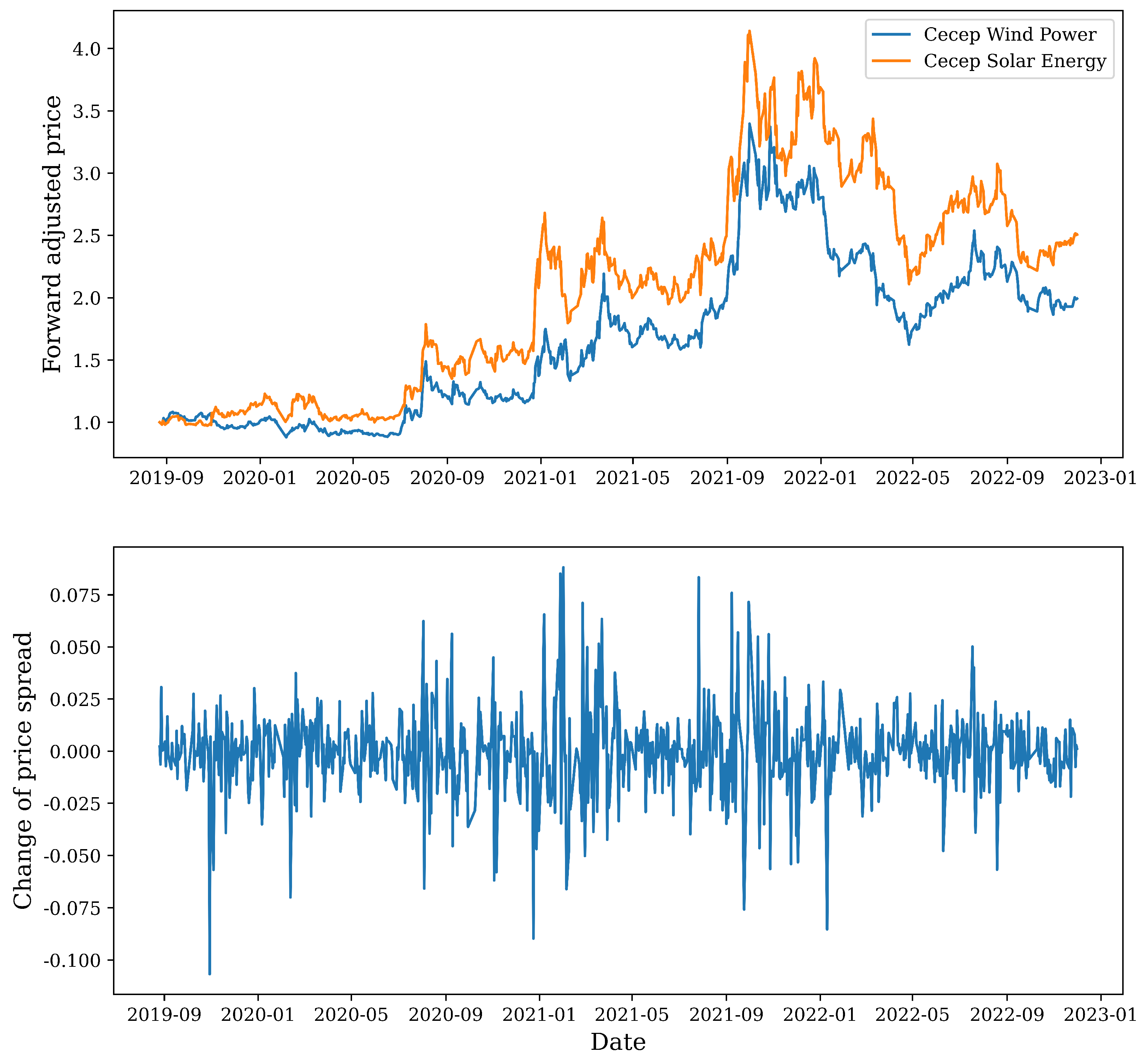
The sample period is from 1 June 2019 to 1 December 2022 across different industries, but the stocks in each pair are in the same industry and are highly correlated in terms of both fundamentals and price series. The data were obtained from TDX software, and we only used the daily closing prices. Typically, we used the forward-adjusted prices to avoid the dividend effect.
Figure 1 presents the forward-adjusted stock prices and the dynamics of the corresponding price spread for the first pair as an example.
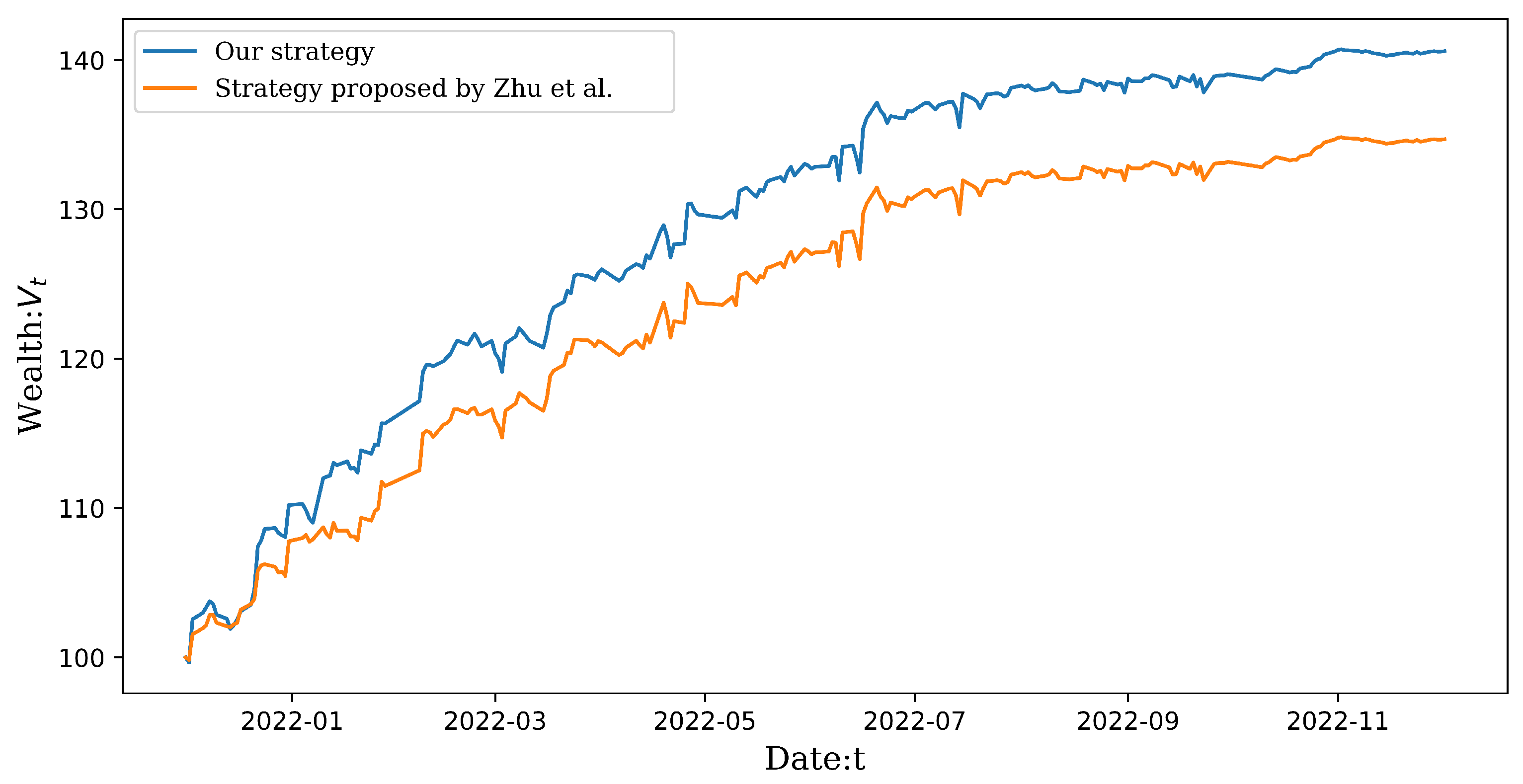
Starting from 1 December 2021, we performed out-of-sample testing for all cases using the moving-window method. Parameters were updated everyday by using data from last 375 trading days (on and a half years). We chose
and equally allocate the initial endowment of 100 units among the selected pairs. The paths of the wealth processes obtained from our strategy under the Scott model and from the strategy proposed by Zhu et al. are shown in
Figure 2, respectively.
Table 2 presents some of the commonly used statistics denoting strategy performance.
Figure 2 and
Table 2 indicate that our strategy under the Scott model outperforms the strategy proposed by Zhu et al. under the constant volatility model with respect to important indicators such as the Sharp ratio, the profit-loss ratio and the win rate in the out-of-sample testing.
To further compare the value of the mean-variance objective function
J for these two strategies, we implemented simulations with respect to the parameters estimated using real market data for the stock pairs listed in
Table 1. Parameters for the simulation are given in
Table 3. As for the strategy proposed by Zhu et al., we used
as the constant volatility, which is the long-term average volatility in the Scott model.
We chose
, and simulated each pair 1000 times with risk aversion
values rangingvaries from
to
. The statistics of the discounted terminal wealth for each pair are shown in
Table 4,
Table 5 and
Table 6.
J is the value of the objective function defined in (
7).
Table 4,
Table 5 and
Table 6 indicate the effectiveness of both strategies by comparing the average terminal wealth with the initial asset
. Both strategies yield a discounted final wealth greater than
in every case, which means that profit is always higher than the risk-free return. Furthermore, comparing the strategy statistics of the strategy proposed by Zhu et al. and our strategy in each case, we found that the standard deviation of the terminal wealth of our strategy is always smaller than that of the strategy proposed by Zhu et al. Although the mean may be lower, ultimately, the
J value of our strategy is always greater than that of the strategy proposed by Zhu et al. This phenomenon suggests that the approximate optimal strategy under the Scott model outperforms the optimal strategy under the constant volatility strategy, by producing more stable profits. It is noteworthy that
plays a critical role in controlling the uncertainty of the outcome result of both strategies. The mean and the standard deviation of the terminal wealth decrease as
increases. Intuitively, a larger
indicates more risk aversion, which leads to smaller allocation on the risky assets and thus lower uncertainty.
Clearly, our strategies show effectiveness for both simulated and real out-of-sample data. The comparison of the strategy proposed by Zhu et al. and our approximate strategy shows that the Scott model can better capture the mean-reverting characteristic of volatility, resulting in a more stable trading strategy.


