Abstract
The slime mould algorithm may not be enough and tends to trap into local optima, low population diversity, and suffers insufficient exploitation when real-world optimization problems become more complex. To overcome the limitations of SMA, the Gaussian mutation (GM) with a novel strategy is proposed to enhance SMA and it is named as SMA-GM. The GM is used to increase population diversity, which helps SMA come out of local optima and retain a robust local search capability. Additionally, the oscillatory parameter is updated and incorporated with GM to set the balance between exploration and exploitation. By using a greedy selection technique, this study retains an optimal slime mould position while ensuring the algorithm’s rapid convergence. The SMA-GM performance was evaluated by using unconstrained, constrained, and CEC2022 benchmark functions. The results show that the proposed SMA-GM has a more robust capacity for global search, improved stability, a faster rate of convergence, and the ability to solve constrained optimization problems. Additionally, the Wilcoxon rank sum test illustrates that there is a significant difference between the optimization outcomes of SMA-GM and each compared algorithm. Furthermore, the engineering problem such as industrial refrigeration system (IRS), optimal operation of the alkylation unit problem, welded beam and tension/compression spring design problem are solved, and results prove that the proposed algorithm has a better optimization efficiency to reach the optimum value.
MSC:
90C27
1. Introduction
The method of optimization involves finding the best global response for a given problem in the search space. Several real-world problems are facing optimization challenges. The need for novel optimization strategies becomes more apparent than before as problems become more complicated. Several approaches have been significantly advanced in the last few decades to solve optimization problems. For example, prior to the development of heuristic optimization techniques, the only method available for solving issues was mathematical optimization. However, these techniques require knowledge of the optimization problem’s properties, such as continuity or differentiability. Metaheuristic techniques have gained increasing momentum in optimization techniques in recent years. Several popular algorithms in this domain are particle swarm optimization (PSO) [1], genetic algorithms (GA) [2], moth flame optimization [3], whale optimization algorithm [4], grey wolf optimization [5], and so on. These algorithms find application in several fields of research and industry as well. Notwithstanding these optimizers’ advantages, the fundamental question is whether an optimizer can solve each optimization problem. In optimization, as stated by the No Free-Lunch (NFL) theorem [6], researchers are permitted to create new algorithms that solve optimization problems more successfully. This makes it accessible to researchers to propose algorithm improvements that are more effective in specific situations, which advances the solution of complex problems in optimization.
Constrained optimization problems (COPs) are optimization problems that are currently in existence but are frequently limited by certain restrictions. Constrained evolutionary algorithms handle constrained optimization problems by combining evolutionary algorithms with constraint-handling technology. Evolutionary algorithms are commonly employed to tackle constrained optimization problems because of their strong universality, robustness, reliability, and low information requirements [7]. Meanwhile, over the past 20 years, numerous algorithm-based constraint-handling strategies have been suggested. Currently, the most popular and straightforward approach for handling constraints is the penalty function method [8], which includes or removes a penalty term from the objective function to change a constrained optimization problem into an unconstrained optimization problem. Since most real-world problems include constraints, it is essential to determine the optimum solution for an optimization problem with constraints, such as resources, time, cost, or design constraints. Slime Mould Algorithm (SMA), a unique bio-inspired optimization method [9], was proposed in 2020 by Li et al. The oscillatory behavior of slime mould during foraging serves as its inspiration. The benefits of the SMA are its excellent scalability, few parameters, and straightforward concepts.
While the SMA has been shown to work exceptionally well, it is not without the limitations. It is unable to find stability between the search trends—exploration and exploitation. This limitation could lead to inadequate solution precision, slower convergence, and an inability to come out of local optimum values. To improve the limitations of the SMA algorithm, this study proposes an enhanced algorithm called SMA-GM that presents a Gaussian mutation (GM) technique for improving SMA. The main contributions are as follows:
- The proposed work designs the Gaussian mutation (GM) scheme, which acts on the current positions of slime mould. The proposed scheme can efficiently boost the local search capability of the optimal position of slime mould and avoid falling into the local optima;
- The greedy selection approach is used for selection purposes to make sure that the slime mould with better fitness enters the next generation, ensures the algorithm’s convergence speed, and preserves population diversity;
- The proposed strategy is verified by using 13 unconstrained and constrained optimization problems and CEC2022 benchmark functions. Furthermore, the comparison of the SMA-GM with the original SMA and with some well-established optimization algorithms has been shown, and the constrained engineering problem is solved through SMA-GM;
- The experimental results, along with the Wilcoxon rank sum test as a statistical test, demonstrate the advantages and the superior performance of the proposed SMA-GM algorithm. The findings prove that the GM approach effectively improves the classical SMA’s search efficiency.
The remaining structure of this paper is organized as follows: Section 2 provides related work. Section 3 presents the preliminaries. In Section 4, the proposed SMA-GM algorithm is explained. Experimental results are given in Section 5. Section 6 includes the mechanical engineering design problem. Lastly, conclusions and directions for further study are presented in Section 7.
2. Related Work
The referenced literature studies show that the researchers have created a wide range of hybrid and metaheuristic versions of SMA to address many kinds of stochastic problems by mimicking the behavior of slime mould in finding out the food source. Yuan L et al. [10] proposed an improved algorithm by embedding elite and chaotic stochastic approaches into the structure of SMA for maintaining better stability among exploration and exploitation stages. Naik et al. [11] enhanced the SMA’s exploration capability by adding a balanced optimizer balanced pool, which improves the SMA individuals’ randomness. Houssein et al. [12] used an adaptive guided differential evolution (DE) algorithm for improving SMA. Yu et al. [13] introduced a quantum-based enhanced SMA, which gives better results in many optimization problems. A hybrid of arithmetic optimizer with SMA was employed by Chauhan S et al. [14] for improving the lesser internal memory and low convergence at local optimal. Zhao J et al. [15] enhanced the searching ability of SMA by replacing random weights through levy flights. Abualigah L et al. [16] proposed an opposition-based learning algorithm to increase the SMA rate of convergence and further levy flight distribution is incorporated with SMA for improving exploration and exploitation stages. Örnek et al. [17] propose the updating of SMA position by imposing the reciprocal oscillation feature of sine and cosine through each generation, which successfully boosts the exploration phase.
Gaussian mutation (GM) is also an optimization algorithm. Researchers have proposed GM as an improvement mechanism to boost the exploration or exploitation function. Yu et al. [18] proposed the quantum revolving door and GM approach for improving the dragonfly algorithm (DA) performance efficiently. Zhang et al. [19] employed fruit fly optimization (FOA) with a GM strategy and a chaotic local search approach for solving problems of feature. Chen et al. [20] proposed improved bacterial foraging optimization (BFO) with GM and a chaotic design for strengthening its performance. To balance exploration and exploitation, Luo et al. [21] developed an enhanced multi-strategy grasshopper optimization algorithm (GOA) with GM, levy flight, and opposition-based learning strategies. An enhanced Gaussian barebone was proposed by S. Wu et al. [22] as the DE mutation extension to improve the update approach of SMA.
3. Preliminary
3.1. Slime Mould Algorithm
With several novel characteristics and a unique mathematical framework that makes use of adaptive weights to simulate positive and negative feedback through bio-oscillator-based propagation waves as best paths for linking food for better exploration and exploitation, the SMA [9] is a novel stochastic optimizer resulting from the slime mould oscillation model in nature. The SMA mimics the behavioral changes that slime moulds undergo when searching for and encircling food during the foraging phase. They have a fan-like morphology at the front, followed by a web of connecting veins. The diffusive waves are created by the slime mould’s bio-oscillator, which modifies the cytoplasmic flow in the veins as they reach the food point and eventually generate the optimal path. The constant z with value 0.03 and transition probabilities are critical parameters for maintaining balance in the SMA. SMA will randomly explore between the bounds set by and when randomly created values are smaller than z. On the other hand, SMA will exploit and search in neighboring areas of the current position if the random value, , is greater than . SMA will wrap around the current best position when is smaller than . The current location’s fit will determine the wrapping direction and radius. The following operations highlight the SMA behavior.
Approach food: For simulating the contraction mode and to represent the approaching behavior of slime mould, the given below rule is presented
where decreases linearly from one to zero and has a range of [−a, a]. indicates the location of the slime mould, , and signify two arbitrarily chosen individuals from the population, means the slime mould weight, and indicates the current iteration. represents the individual position with the maximum odor concentration. The following is the formula:
The following is the formula for and :
where indicates the smell index, i.e., it is the sorted order of fitness values; signifies the optimum fitness found in the current iterative manner, presents the poorest fitness value found in the iterative course, and shows that ranks the first half of the population and that the random value in the interval [0, 1] is denoted by .
Wrap food: The mathematical strategy given below is applied for updating the location of slime mould
where and indicate the arbitrary value in [0, 1] and , indicates the lower and upper boundaries of the search range, and is the parameter taken as 0.03.
Oscillation: With the increasing number of iterations, the value gradually approaches zero and oscillates arbitrarily between [−a, a]. oscillates from [−1, 1] and ultimately tends to zero. The pseudocode of SMA is presented in Algorithm 1.
| Algorithm 1: Pseudocode of SMA |
Begin
|
| Calculate the fitness of all slime mould |
| Calculate the W by Equation (4) |
| For |
| Equation (6) |
| End for |
|
| End |
3.2. Gaussian Mutation
The popular optimization technique that works well at the exploitation stage is the Gaussian mutation (GM). The Gaussian distribution, represented by , where and are the variable’s mean and standard deviation, is widely employed in statistics and the natural sciences to represent real-valued random variables. Gaussian distribution includes the renowned rule, which provides a chance for foraging depending upon the requirement of the problem. Gaussian distribution has been widely utilized in the literature to modify control parameter values but it is rarely employed to create new mutation operators to retain a robust local search capability while increasing diversity. The GM operator is used to enhance the SMA to exploit the benefits of the Gaussian distribution fully. The Gaussian probability density formulation is represented in the following way:
The scheme GM is expressed in the following way
where is the parameter’s current value and represents the arbitrary value from Gaussian distribution with mean 0 and standard deviation GM is the mutation operation that introduces population variability and explores the search space. When using GM, the original population is replaced with an arbitrary number that satisfies the variance and mean values. The GM scheme emphasizes a local area close to the original individual based on the normal distribution characteristics and it has demonstrated excellent efficiency in various optimizers.
4. Proposed Methodology
SMA has limitations even though it performs competitively when compared to other algorithms. The reduced population diversity of SMA enables it to enter the local optimum quickly. As the problem grows more complex and converges more slowly in subsequent iterations, SMA finds it challenging to balance exploration and exploitation. To further boost the performance of SMA and considering that the NFL inspires us to enhance the existing algorithms’ performance, Gaussian mutation (GM) is proposed to strengthen the SMA’s search capability and to achieve local and global optimality and is named the SMA-GM algorithm. Back and Schwefe [23] proposed using the Gaussian mutation (GM) to increase the search efficiency of heuristic algorithms. In general, GM produces new solutions that are near the candidate solutions. When the search is being conducted, it explores the search space in small steps, increasing the diversity of the population. Random perturbations are introduced to the current solution based on a Gaussian (normal) distribution. The proposed SMA-GM holds a better position when compared with the target value of the current optimum individual solution. The algorithm produces well-balanced local and global results because of the proposed strategy. A random variable is created by taking the mean of zero and the standard deviation of one. The Gaussian distribution function can be expressed as follows:
where the variance value of the candidate solutions is σ2. To thoroughly study the features of the current population, two locations are arbitrarily selected, and their difference is considered to link with the Gaussian distribution operator to construct the proposed GM mechanism. The following is the presentation for GM strategy:
where is the Gaussian distribution mechanism of Equation (9), and is the optimum location for the current iteration of the original SMA. Following the GM operation, the new position is presented by . The positions of the two slimes selected randomly from the population are represented by and , respectively. The value of oscillates randomly between and approaches with increasing iterations. In order to further balance the exploitation and exploration and making the smooth oscillation process, the parameter is updated as follows:
where, is a dynamic parameter adaptively adjusted with the number of iterations. indicates the current iteration and indicates maximum number of iterations. Algorithm 2 displays the proposed algorithm’s pseudocode after the normal execution of SMA while updating the parameter . The optimum location is mutated to create a new mutated solution using the GM process through Equation (10).
| Algorithm 2: Pseudocode of the SMA-GM algorithm |
Begin
|
| Calculate the W by Equation (4) and a by Equation (11) |
| For |
| Equation (6) |
| Update the position of the slime mould and the optimal position as |
| Gaussian mutation mechanism |
| by Equation (12) |
| Update optimal solution to |
| Replace the parent slime with the generated mutant slimes if its fitness is found to be better. |
| End If |
| End For |
|
| End |
The new mutated solution is then compared to the optimal position of the original SMA to determine whether the new mutated solution is still the better solution and if not, the optimal position of the original SMA is updated to the optimal solution through a greedy selection mechanism. Individuals who have better fitness are selected to enter the next iteration. The computing process for this is shown below.
The pseudocode of SMA-GM illustrates how the proposed method reconsiders the position details following the original algorithm’s search for a feasible outcome. The above-mentioned technique not only broadens the population’s diversity but also boosts the effectiveness of the search process; in the process, the enhanced version keeps the original algorithm’s structure relatively straightforward. SMA-GM consists of the subsequent parts for complexity, such as initialization, fitness evaluation, sorting, weight update, position update, Gaussian mutation, and greedy search. Among them, represents the number of slime mould, represents the dimension, and represents the maximum number of iterations. The total complexity of SMA-GM is . Figure 1 presents the flowchart of the SMA-GM algorithm.
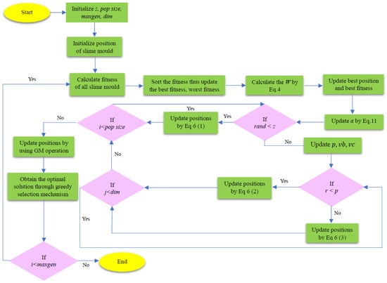
Figure 1.
Flowchart of the SMA-GM algorithm.
5. Experimental Setup and Results
Optimization problems are generally categorized into two: unconstrained and constrained. The optimization method in the unconstrained problems seeks for an objective function’s minimum or maximum possible value. Since the optimal solution for the second kind of problem must meet the constraints specified for the problem, the method is more complex. In simple words, the solution ought to be feasible. To verify the performance of SMA-GM, the results of the proposed algorithm are compared against four state-of-the-art algorithms from the literature, including SMA [9], GWO [5], MFO [3], and WOA [4] and two more improved optimization algorithms are included for fair comparison, which are AGWO [24] and IChoA [25]. The parameter settings of these algorithms are given in Table 1. The environmental conditions are an 11th Gen Intel(R) Core (TM) i3-1125G4 @ 2.00GHz, 8.00 GB of RAM and the Windows 11 operating system and the simulation experiments are set up on the MATLAB R2021a platform. The SMA-GM algorithm was evaluated and compared with other algorithms using 38 functions, including 13 unconstrained, 13 unconstrained (F1–F13), constrained benchmark functions (G1 to G13), and CEC2022 benchmark functions. The “Mean”, “St.dev”, “Best”, and “Worst” values of the objective function are given after each problem was run 30 times and the number of iterations of each algorithm was fixed to 1000 with a population size 30 and the maximum number of function evaluations is set to 30,000.

Table 1.
Parameter setting of the involved algorithms.
5.1. Unconstrained Benchmark Functions
This section includes the 13 benchmark functions that were utilized for the experiments. These functions are categorized as unimodal (F1–F7) and multimodal functions (F8–F13). The unimodal functions are employed for testing an algorithm’s potential for exploitation. Conversely, the ability to explore and the stability of algorithms can be found in the multimodal test functions that have a large number of local minima. For each function, the experiment is carried out for 30, 60, and 200 dimensions and the search range of all the functions is set to [−100, 100]. The main parameter values of each algorithm are listed in Table 1 and Table 2 lists the summary of unimodal and multimodal test functions. It should be noted that SMA-GM employed the same parameter values as the original algorithm. As such, it could offer a guarantee of stability in the proposed algorithm’s performance. Additionally, for a fair comparison, the test conditions were the same as those listed in Table 1.

Table 2.
Summary of unconstrained benchmark functions.
5.1.1. Exploration and Exploitation Analysis
Table 3 displays the results of the unimodal and multimodal test functions. According to the experimental findings, SMA-GM performs better in most of the test functions. Most notably, SMA-GM achieved satisfactory results in both low and high dimensions for the unimodal functions (F1–F7). In all three dimensions, SMA-GM is able to consistently achieve the theoretically optimal solutions for F1 and F3. In comparison, the other comparable algorithms are not very capable of achieving the theoretical optimal value in all the test functions and perform weaker than SMA-GM. Comparing the test results of each dimension, the results show that the SMA-GM’s performance has not dropped too much with increasing dimensions, which illustrates that SMA-GM has outstanding local exploitation capability. For the multimodal functions (F8–F13), the SMA-GM steadily achieves the theoretical optimal values at F9–F11 in all three dimensions (30, 60, and 200). SMA-GM has the overall best performance in the multimodal functions, signifying that the improved algorithm extensively boosts the global exploration capability of SMA.

Table 3.
Results of the unconstrained benchmark function in different dimensions.
5.1.2. Convergence and Scalability Analysis
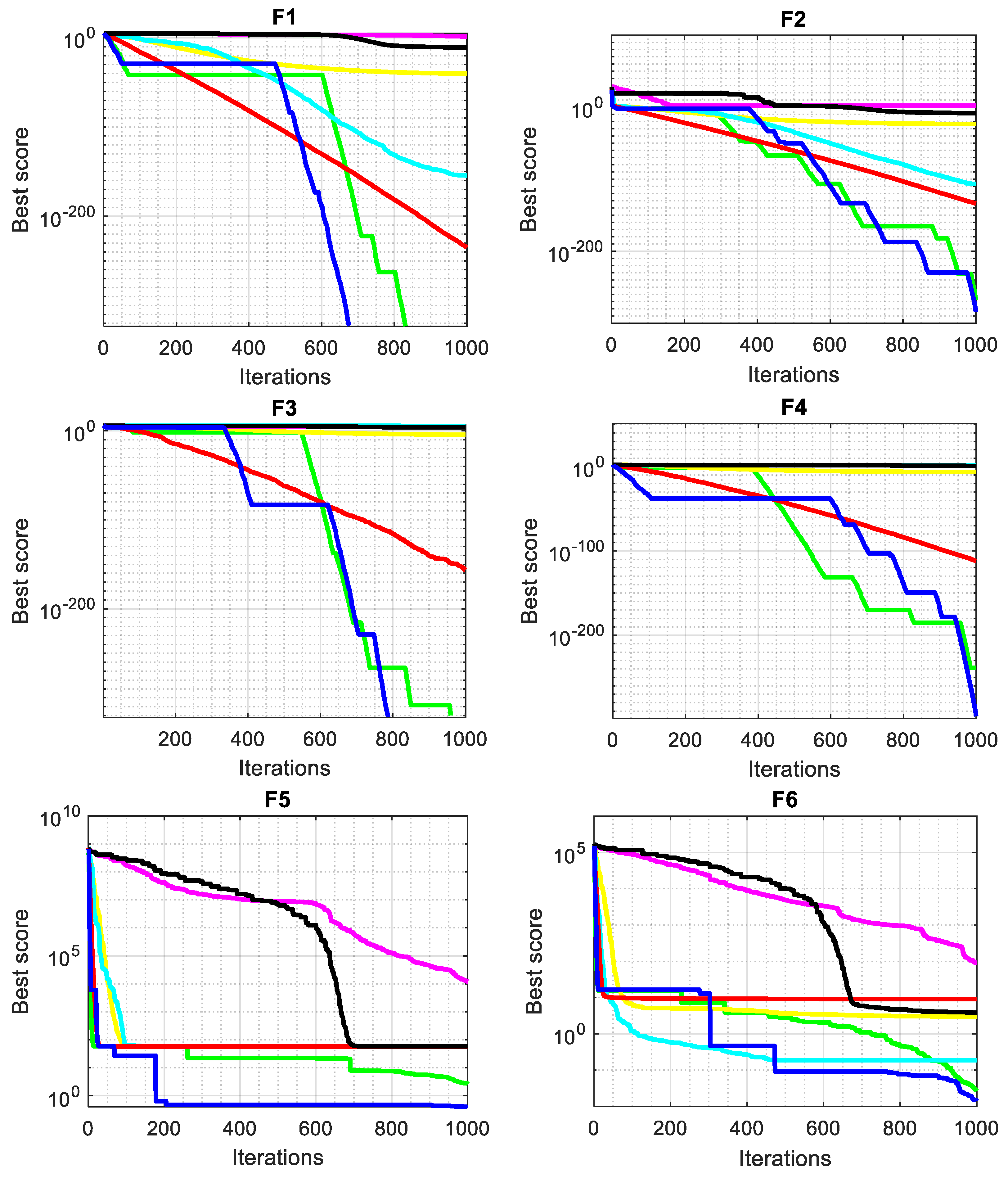
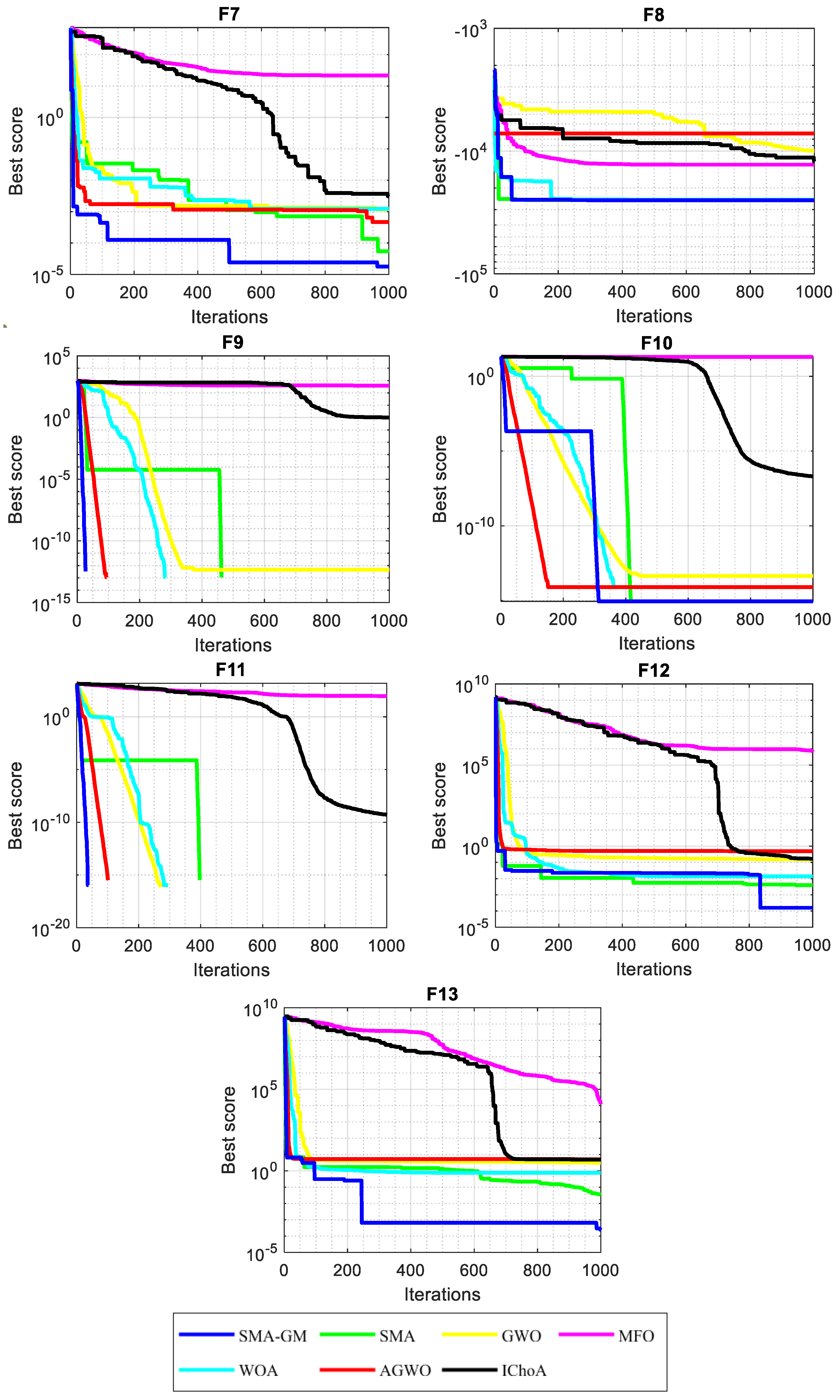
In order to study the convergence performance of SMA-GM, convergence curves are plotted according to the results with 60 dimensions, as given in Figure 2. In unimodal functions, the curve is smooth and continuously decreasing, demonstrating the algorithm’s ability to find the optimal solution. For multimodal functions, the convergence curve descends in steps, signifying the algorithm’s capability to steadily escape local optima and reach the global optimum. At the beginning of the iteration, the decline speed for F1, F2, F4, and F10 of SMA and AGWO in the convergence curve is faster than that of SMA-GM. But in the later stage of the iteration, SMA-GM exceeds SMA and AGWO, indicating the robust development ability of the proposed algorithm. Therefore, the improvement strategy proposed in this paper can successfully enhance the convergence speed of SMA and achieve better optimization results.

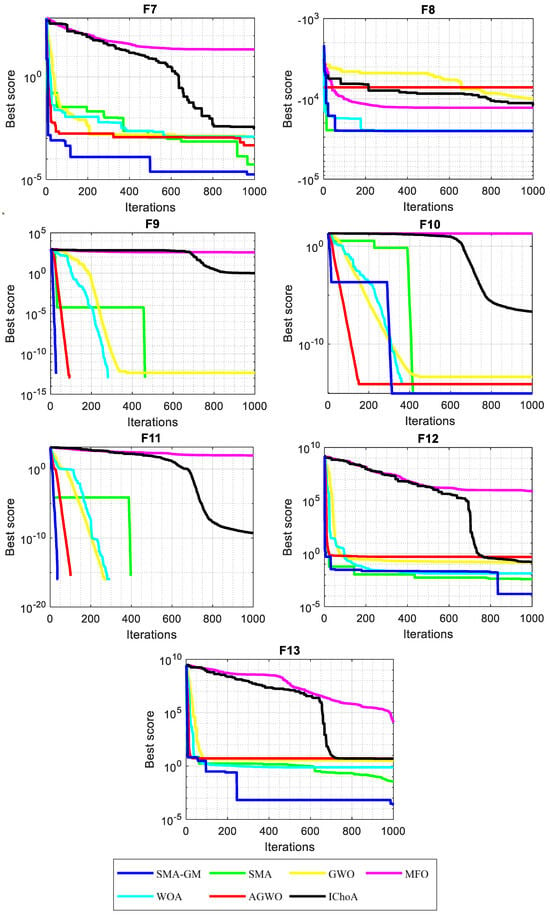
Figure 2.
Convergence curves of unconstrained benchmark functions with 60 dim.
The scalability test reveals the performance fluctuation of optimization algorithms. In this study, the performance of SMA-GM in various dimensions (dim = 30, 60, 200) was also tested. It is evident that the algorithm will have greater difficulty in locating the global optimal solution for the higher dimension. Notably, all other experimental parameters were constant in accordance with the aforementioned descriptions, with the exception of the dimension setting. The experiments’ mean value (mean) and standard deviation (Std) are used to measure the results and Table 3 displays the experimental results. A particular algorithm’s quality and accuracy are indicated by its mean value, while its stability is indicated by its standard deviation. The results of the unimodal and multimodal functions both showed that SMA-GM performed exceptionally well in higher dimensions. SMA-GM outperformed SMA and other well-known algorithms in all of the functions except F6. It should be mentioned that these comparison algorithms (GWO, MFO, WOA, AGWO, and IChoA) usually showed weak optimization capabilities, particularly in higher dimensions where the algorithms’ performance fluctuates with increasing dimensionality. Hence, the proposed SMA-GM performed more consistently with better optimization behavior when handling high-dimensional problems.
5.1.3. Diversity Analysis
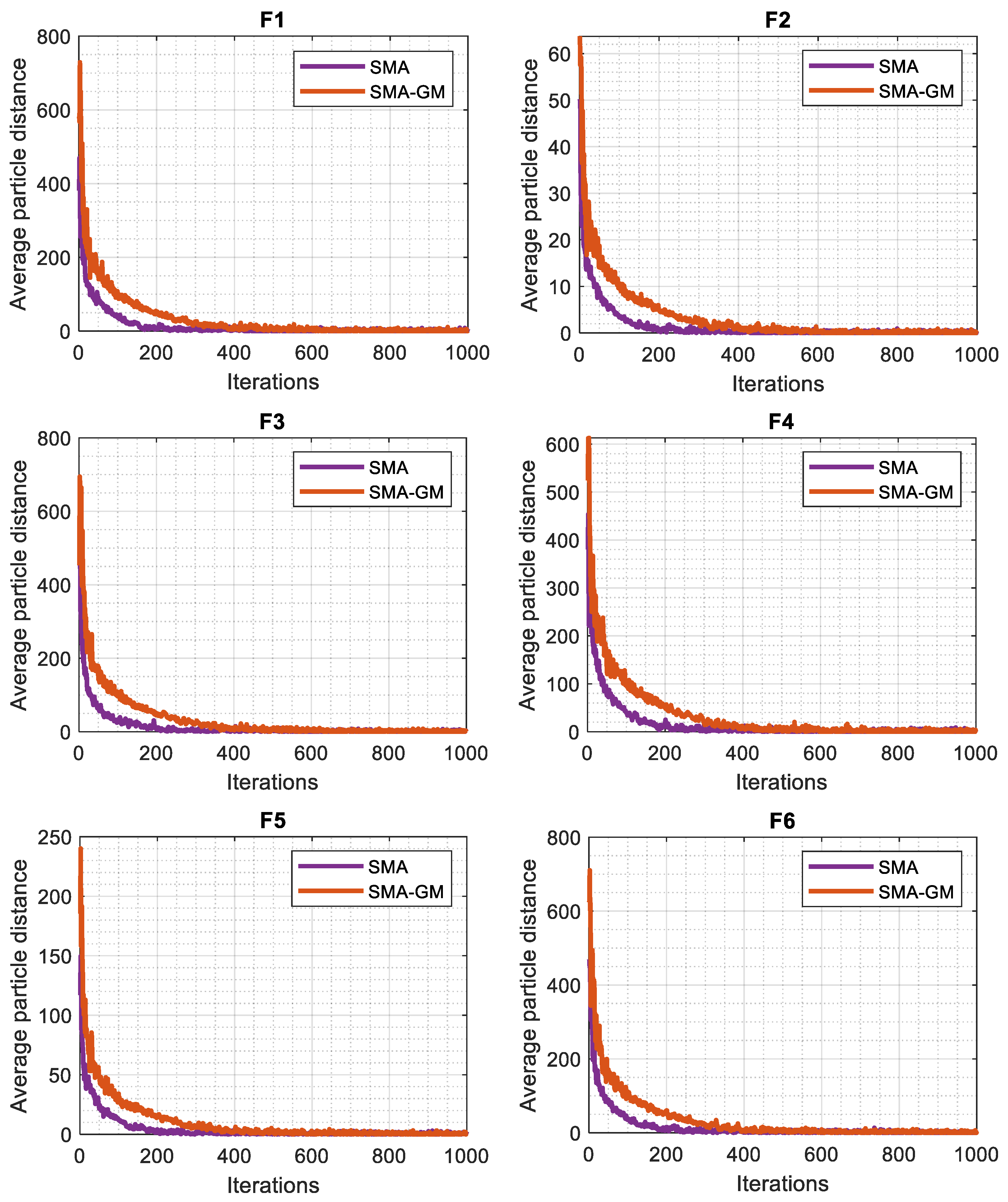
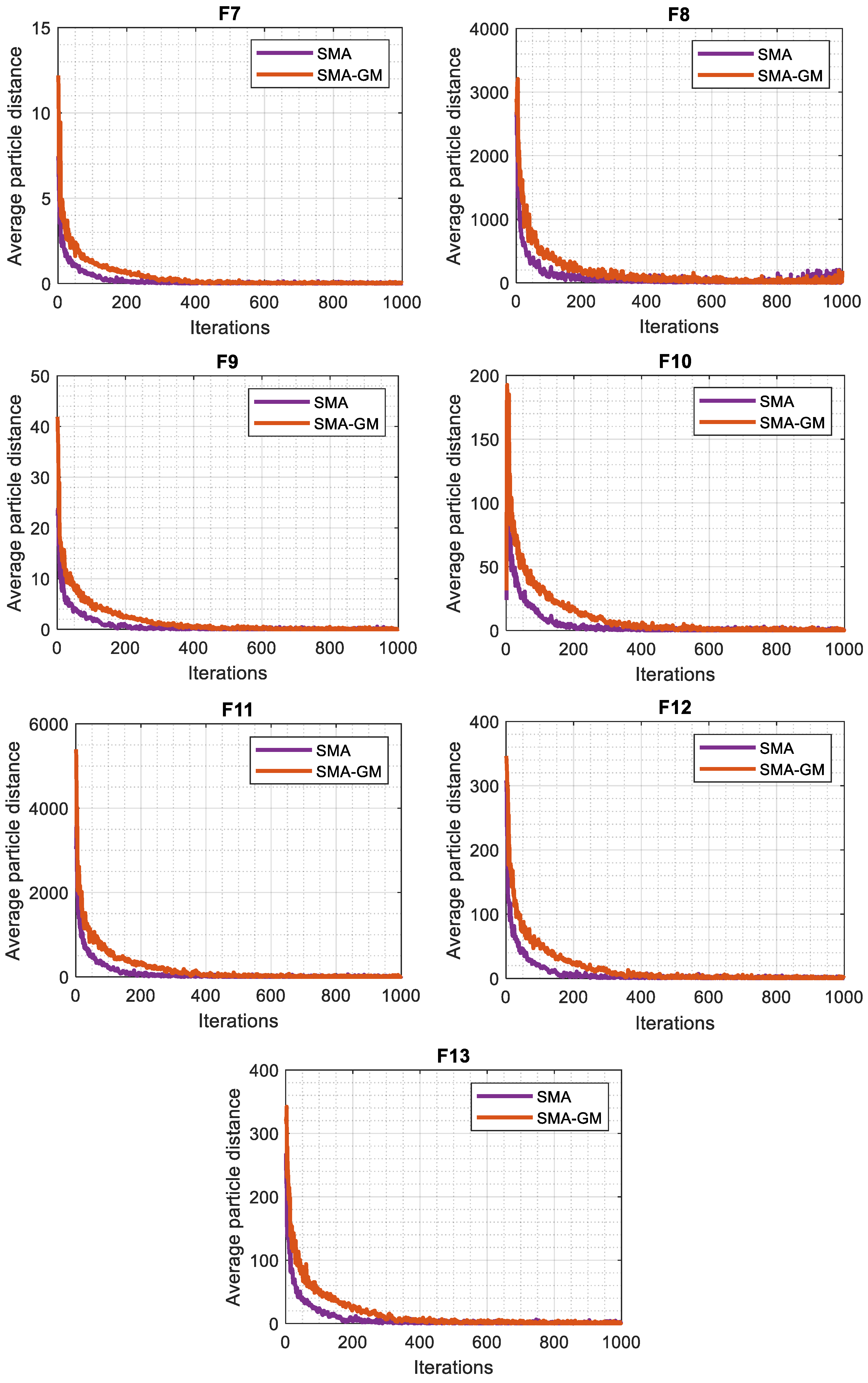
Generally, the algorithm that gives priority to the exploitation phase will have a high convergence rate but there would be a risk of trapping into the local optima. However, the algorithm that focusses more on the exploration phase finds the more search space and the chance of finding the global solution increases though the convergence rate may be weak. Thus, a rationally working algorithm attempts to maintain the balance between these two phases. The diversity test is one of the methods for balance analysis between these two phases. The diversity curves, as seen in Figure 3 for unconstrained functions, indicate the average distance between the search agents during the iterations. The diversity is derived using the following equations, which were inspired by certain studies [26,27]:
where is the number of search agents, indicates the dimension of the problem, presents the dimension of search agent , and presents the median of dimension of the total population.
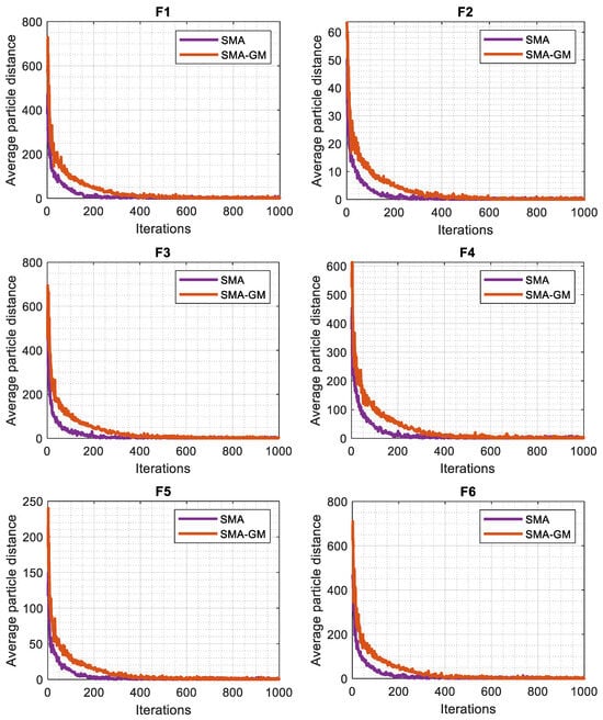
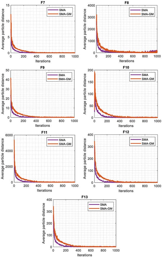
Figure 3.
Diversity analysis of SMA and SMA-GM.
The diversity in each dimension is defined as the distance between the dimension of each search agent and the average median of the dimension. The variation in diversity between the original SMA and SMA-GM is shown in Figure 3. The average distance between the search agents is displayed on the vertical axis, while the number of iterations is displayed on the horizontal axis. Because of the random initialization process, it is evident that both algorithms reflect high diversity in the initial phase of the execution. Then, as a result of various algorithmic operations, the diversity varies. As the iterations increase, the search agents traverse the whole search space and the average distance gradually becomes smaller, making the diversity decrease, and the algorithms gradually go into the exploitation phase, which is consistent with the above analysis. However, in most of the test functions, the average distance in each iteration is high for the SMA-GM algorithm as compared to SMA, which shows the better ability of search in the SMA-GM in terms of exploring new search regions of the search space. This shows the effect of improving the search mechanism of slime moulds through the GM strategy in the SMA-GM algorithm.
5.2. Constrained Handling Technique
The intelligent constrained handling strategy must use the constraints (restrictions) conditions during optimization to optimize the constrained problems [28,29]. The method of including a penalty to the objective function’s value is employed in this article. Equations (16)–(19) were applied for this purpose. The constraint and objective function values are denoted by the parameters and , respectively, in these equations. Furthermore, the constraint values are for the inequality and for the equality constraints. Here, is the solution vector. Additionally, the number of inequality and equality constraints is and , respectively, and the whole constraint is . In this study, 1E-04 is the small tolerance for the parameter.
5.3. Results and Discussion on Constrained Functions
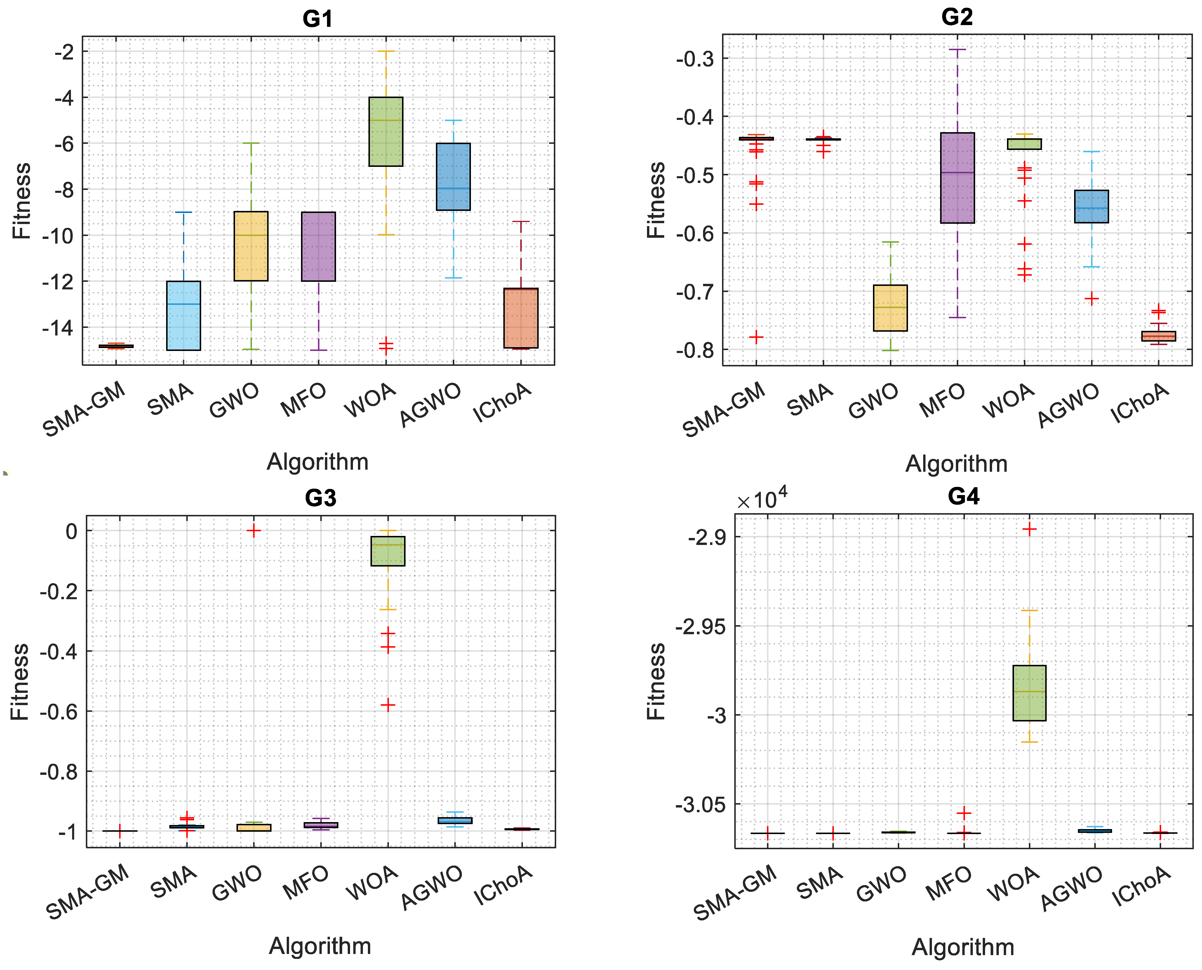
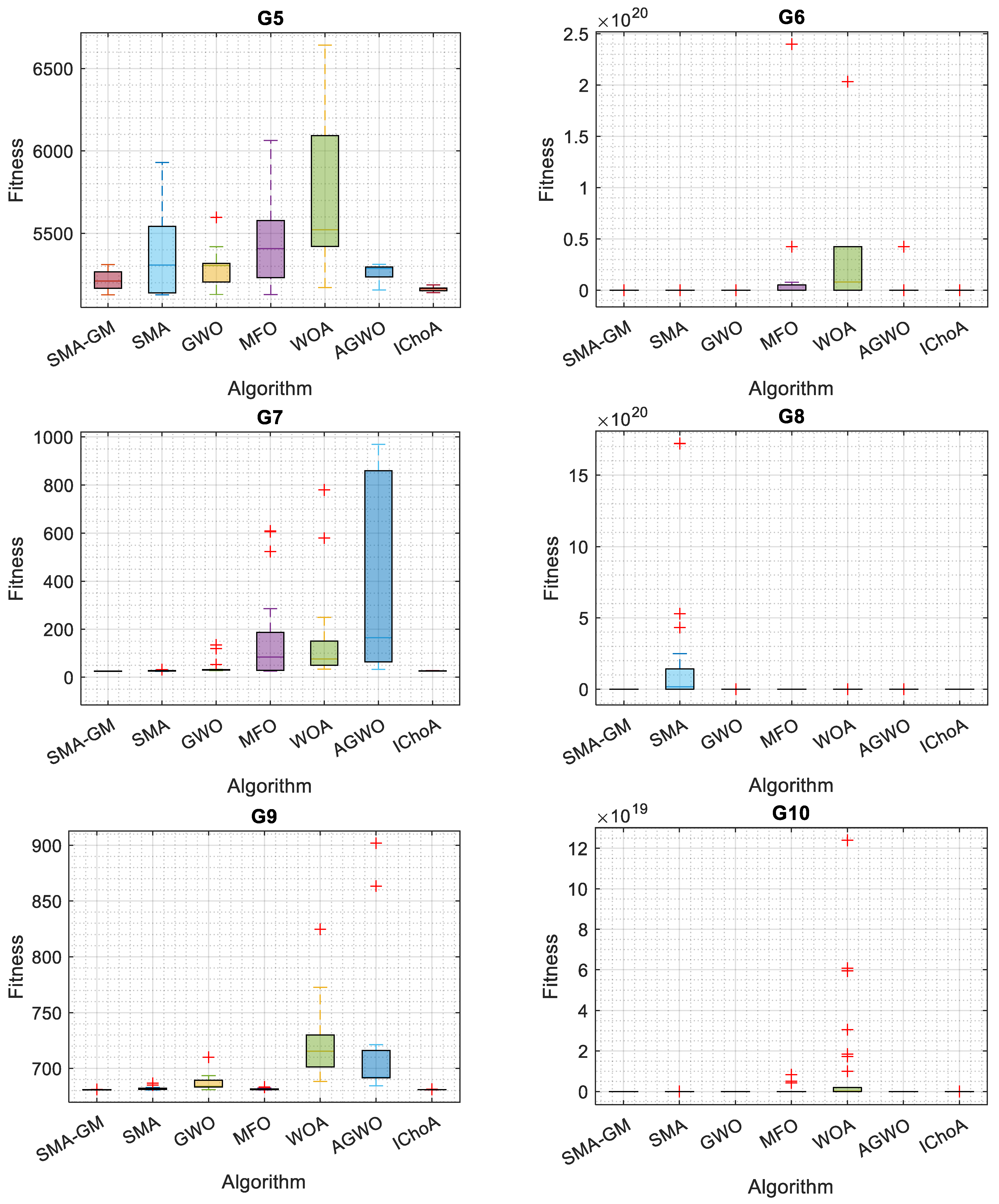
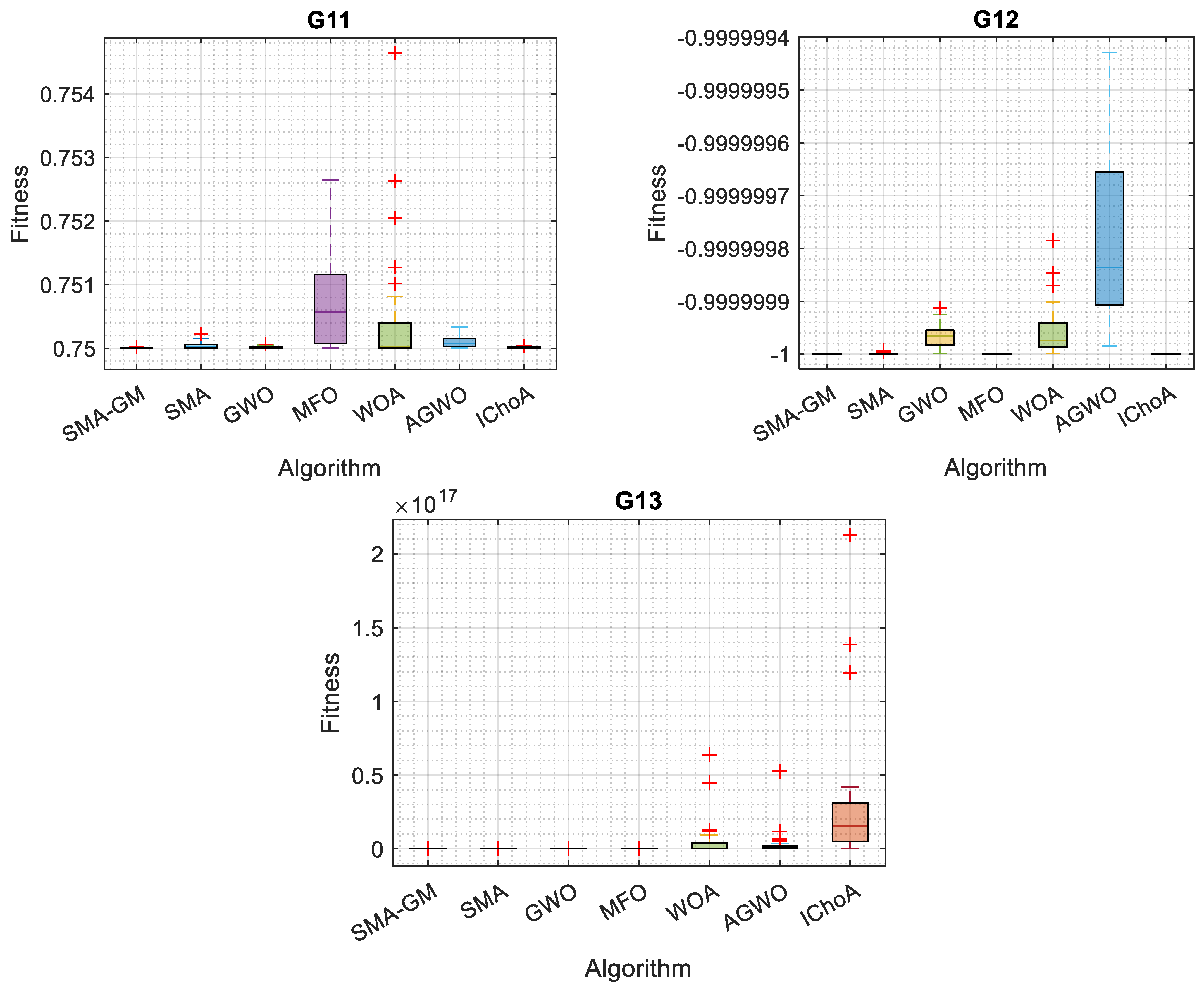
Considering 13 commonly used constrained benchmark functions, the proposed SMA-GM’s capability to handle constrained problems was evaluated. Table 4 shows the different linear, non-linear, and quadratic equations for each problem in the set that take the form of equality and inequality constraints. Table 5 illustrates the results for each constrained benchmark function employed with SMA-GM and other algorithms. The results clearly illustrate that SMA-GM outperforms all other algorithms for 10 of the 13 constrained benchmark functions with excellent efficiency, showing the superiority of the proposed algorithm. IChoA outperformed SMA-GM in the G2 problem; in the G8 problem, SMA-GM performed better than SMA but could not outperform the other algorithms for the G8 problem and for the G5 problem, IChoA performed better than SMA-GM. For problem G11, compared with SMA, GWO, and IChoA, SMA-GM obtained similar results and for the G12 problem, SMA-GM, MFO, and IChoA acquired identical results. The algorithm has produced satisfactory results, either optimal or nearly optimal. According to the results, the proposed Gaussian mutation (GM)-based SMA-GM outperforms the competitive metaheuristic techniques in terms of solution accuracy except for the G2, G5, and G8 problems. Boxplots in Figure 4 strengthen the conclusion mentioned above. The SMA-GM algorithm demonstrates excellent robustness for handling constrained problems, as evidenced by the lowermost position and least height of the box, which is plotted by the obtained outcomes.

Table 4.
Summary of constrained benchmark functions.

Table 5.
Comparison results of constrained benchmark functions.
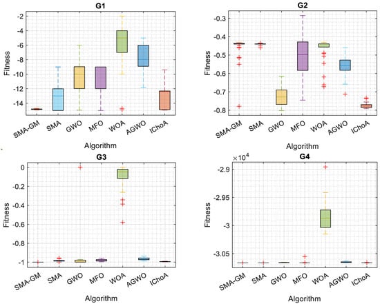
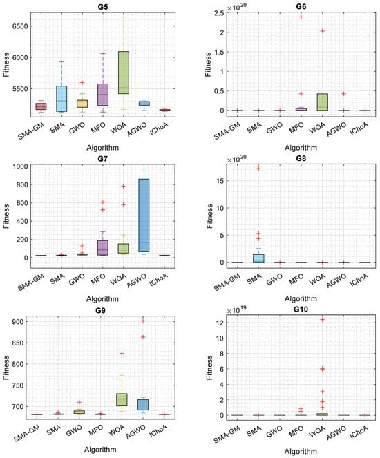
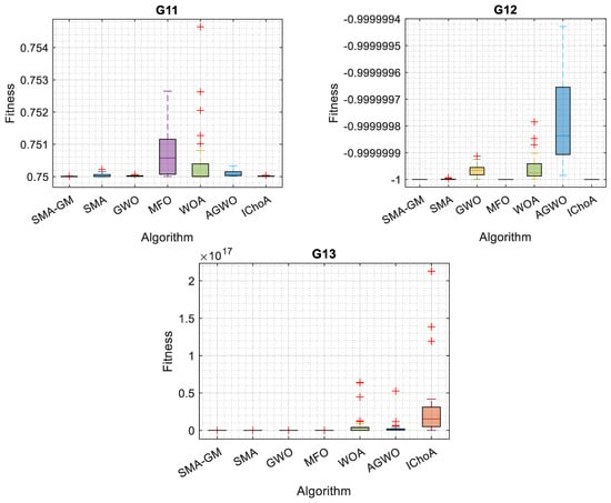
Figure 4.
Boxplot of the SMA-GM algorithm and other algorithms on constrained functions.
5.4. Results and Discussions on CEC2022 Benchmark Functions
In this section, the most recent CEC2022 test functions are selected to further evaluate the performance of the proposed SMA-GM and compare it with other above-mentioned algorithms. The highly complex global optimization problems are simulated by the CEC 2022 test function [30]. All functions were tested in 20-dimensional space to guarantee the validity and fairness of the experimental results. In total, 12 test functions, 4 of which are classified as compositional, unimodal, essential, and hybrid, are included in Table 6 as the summary of CEC2022. The algorithm parameter values used were the same as those listed in Table 1. Table 7 presents the mean and standard deviation (Std) for 30 independent runs, illustrating the higher performance of SMA-GM for 10 out of the 12 test functions in the CEC-2022 test suite. By analyzing the results, it is clear that SMA-GM has satisfactory exploration and exploitation abilities to solve optimization problems. Compared with other algorithms, its optimization accuracy, solution stability, and adaptability to different functions have noticeable advantages and SMA-GM has gained more competitive results.

Table 6.
Description of CEC2022 functions.

Table 7.
Comparison results of SMA-GM with other algorithms for CEC2022 functions.
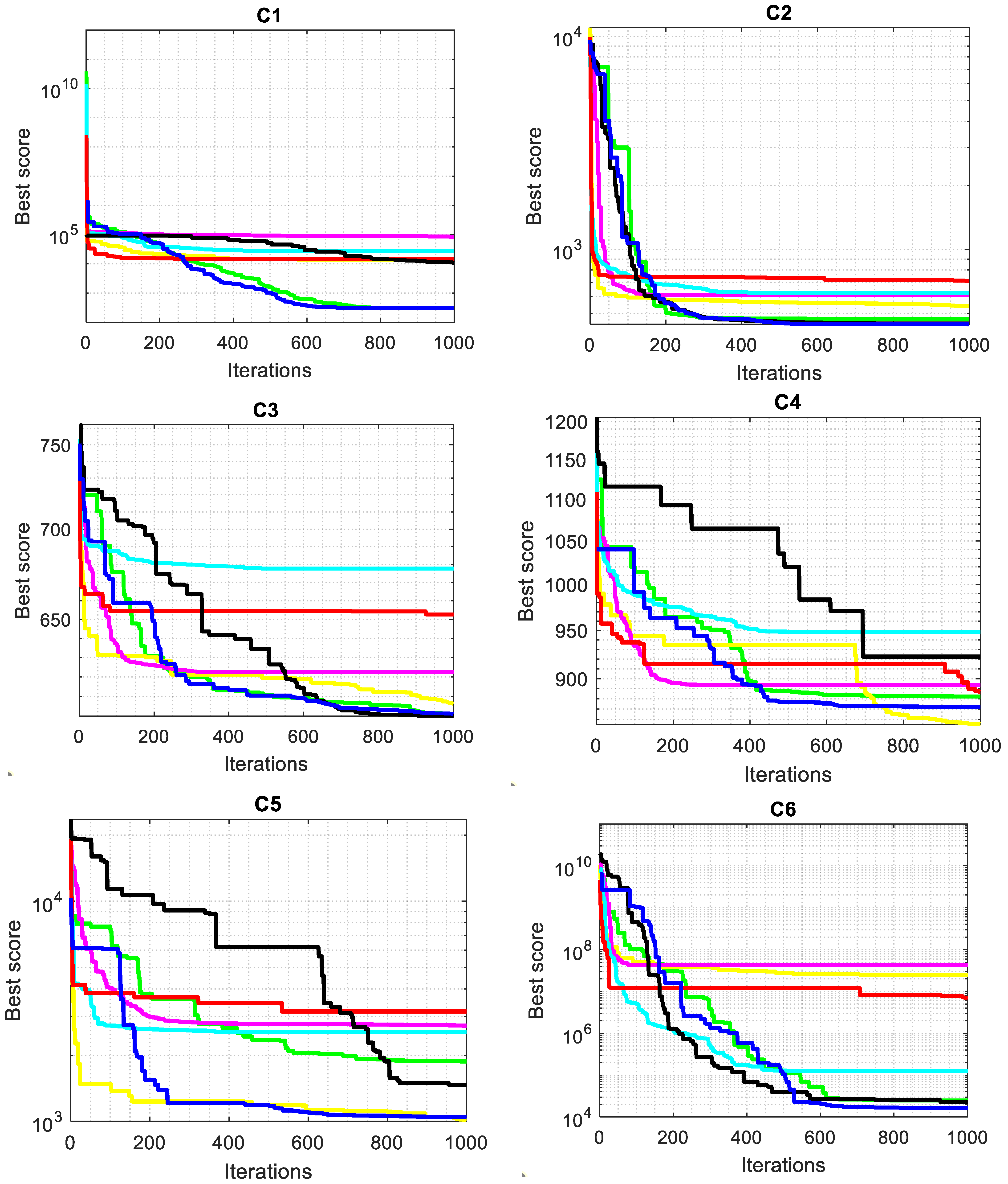
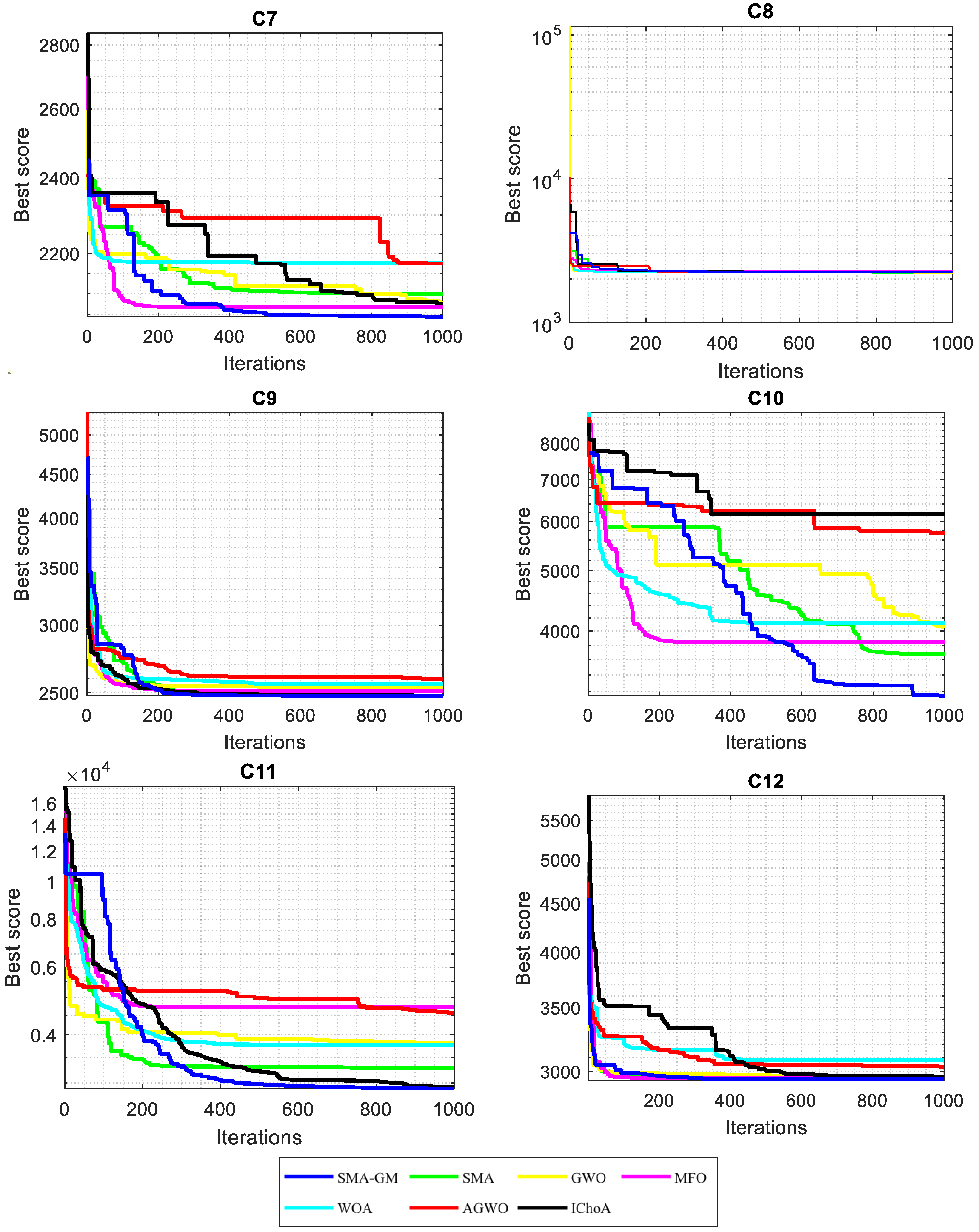
As seen in Figure 5, the convergent graphs are extracted from the CEC2022 test functions to thoroughly validate the SMA-GM algorithm’s performance. The convergence curve shows that whereas other algorithms enter local optima too early, SMA-GM has a faster rate of convergence in the functions C1–C3 and C6–C12. In order to prevent stagnation into local minima, SMA-GM’s performance first explored the majority of the search space. Later, it gradually switched to the exploitation operator to quickly reduce diversity during the second half of the optimization process, speeding convergence toward the most promising region so far found. Due to the search process variation, the SMA-GM performs well, which allows the algorithm to have a strong exploration and exploitation operator during the optimization process. The GM operator helps to preserve population diversity, prevents the system from becoming stuck in local optima, and speeds up the convergence towards the best-so-far solution.
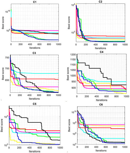
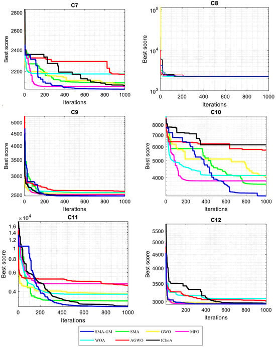
Figure 5.
Convergence curves of CEC2022 benchmark functions.
5.5. Wilcoxon Rank Sum Test
The statistical analysis of the significant difference between the two methods can be conducted using the non-parametric Wilcoxon rank sum test [31]. The Wilcoxon rank sum test method is employed in this study to evaluate if the experimental findings of the SMA-GM algorithm and the counterpart algorithms differ significantly from one another. The results of each algorithm running independently 30 times on the 13 constrained functions (G1–G13) and CEC2022 test functions listed above provide the data utilized in the rank sum test. The rank sum test p-value between SMA-GM and each comparison algorithm is displayed in Table 8. The null hypothesis is rejected when the difference between the two algorithms is significant (p < 0.05). In Table 8, the denotes the independent results obtained from SMA-GM and its corresponding optimizer are identical. The majority of p-values shown in Table 8 is less than 5%, which indicates that the alternative hypothesis is accepted. Hence, the outcome of SMA-GM is different from those of the other compared algorithms. Thus, SMA-GM is a robust optimizer, as verified by its capability to overcome SMA, GWO, MFO, WOA, AGWO, and IChoA, which are the most competent and highly cited metaheuristic optimizers.

Table 8.
Wilcoxon rank sum test results (p-values) of SMA-GM with each algorithm for the constrained function and CEC2022 test function.
6. Constrained Engineering Design Problem
The goal of developing and improving any stochastic search algorithm is to find solutions to real-world problems. In the preceding section, the SMA-GM efficacy was studied through numerical constrained experiments. This section evaluates the exploration and exploitation abilities in real-life situations using the SMA-GM algorithm. In this section, the SMA-GM algorithm is used to solve mechanical engineering design problems, such as the industrial refrigeration system (IRS) design problem, optimization of the alkylation unit procedure, welded beam, and tension/compression spring design problem.
6.1. Optimal Design of an Industrial Refrigeration System
Solving engineering design problems aims to provide the best possible design scheme while taking into account a variety of constraints. SMA-GM is compared with the metaheuristic algorithms mentioned above and the same parameter settings are listed in Table 1. Nowadays, energy saving and emission reduction work has become the focus of several fields. IRS accounts for a large proportion of energy consumption, so it is essential to optimize and control the IRS [32]. The optimal design of IRS is a highly complex mechanical engineering design problem, which has 14 design variables and 15 constraints. Below is an illustration of its mathematical formulation.
- Minimize
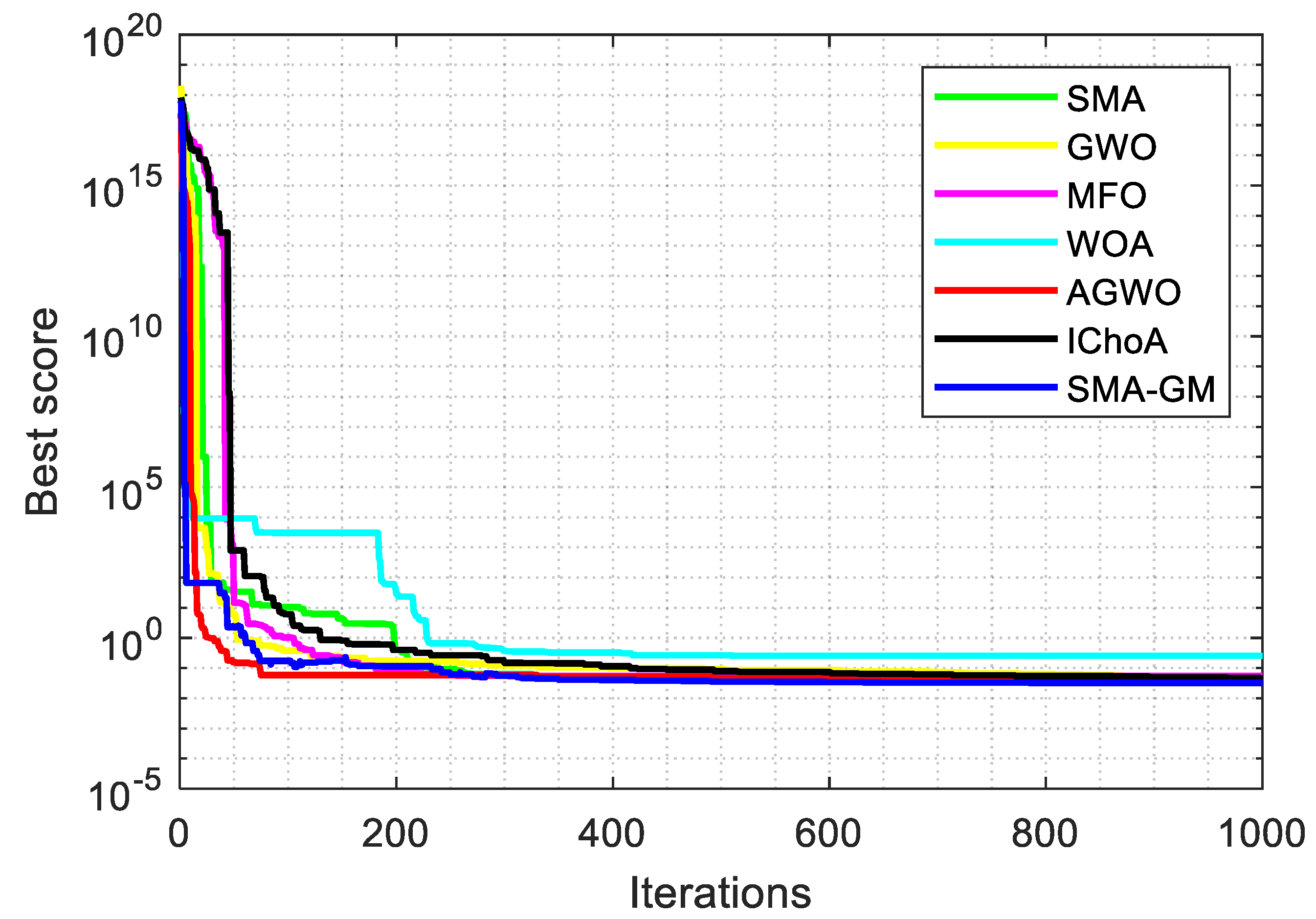
Table 9 compares the results of SMA-GM with the other four optimizers to show which one is best at solving the IRS design problem. Table 10 presents the optimal constraint values. These findings show that SMA-GM outperforms the other optimizers and converges faster than the other optimizers, as shown in Figure 6.

Table 9.
Optimal design of IRS.

Table 10.
Constraint values of the IRS design problem.
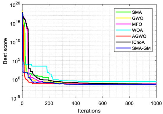
Figure 6.
Convergence curve for IRS.
6.2. Optimal Operation of an Alkylation Unit
The optimal operation of an alkylation unit is very common in the petroleum industry [33]. In the alkylation process, the reactor is filled with the olefin feedstock (100% butane), pure isobutane recycling, and 100% isobutene supplement, along with the acid catalyst. The reactor product is then sent through a fractionator to separate the isobutene and alkane. Additionally, spent acid, the base product, is taken out of the reactor. The alkylation product is the objective function and the primary goal of this problem is to raise the octane number of the olefin feedstock in acidic conditions. This is a complex optimization problem with 14 constraints and 7 variables. Below is an illustration of its mathematical formulation.
- Maximize
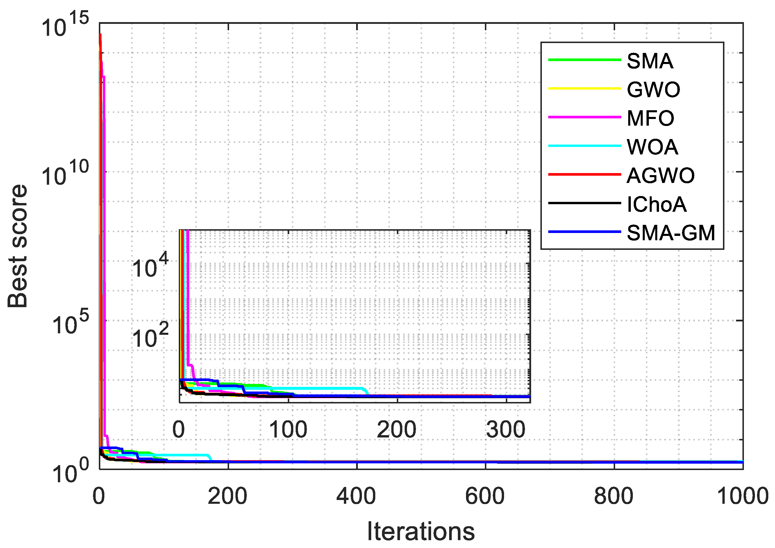
Table 11 shows that the SMA-GM algorithm performs better than other algorithms, signifying that it can maximize the alkylation product value and has a better result for the optimization of the alkylation process. The convergence curve for the optimal operation of the alkylation unit is shown in Figure 7 and Table 12 shows the constraint values. It can be seen from the Figure that the convergence performance of the proposed algorithm is not optimal at the initial stage. But at the later stage of the iteration, the SMA-GM algorithm can get rid of the local optima and continue exploring to improve the overall optimization performance.

Table 11.
Optimal operation of an alkylation unit.
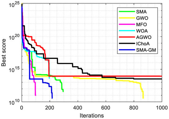
Figure 7.
Convergence curve for the optimal operation of an alkylation unit.

Table 12.
Constraint values of the optimal operation of an alkylation unit.
6.3. Welded Beam Design
The objective of the problem is to construct a welded beam [33] with minimal cost under the bounds of buckling load (), end deflection of the beam , bending stress , and shear stress . It considers the weld thickness , the joint length the height of the beam, and the thickness as variables and the mathematical formulation of this problem is shown as follows:
- Consider
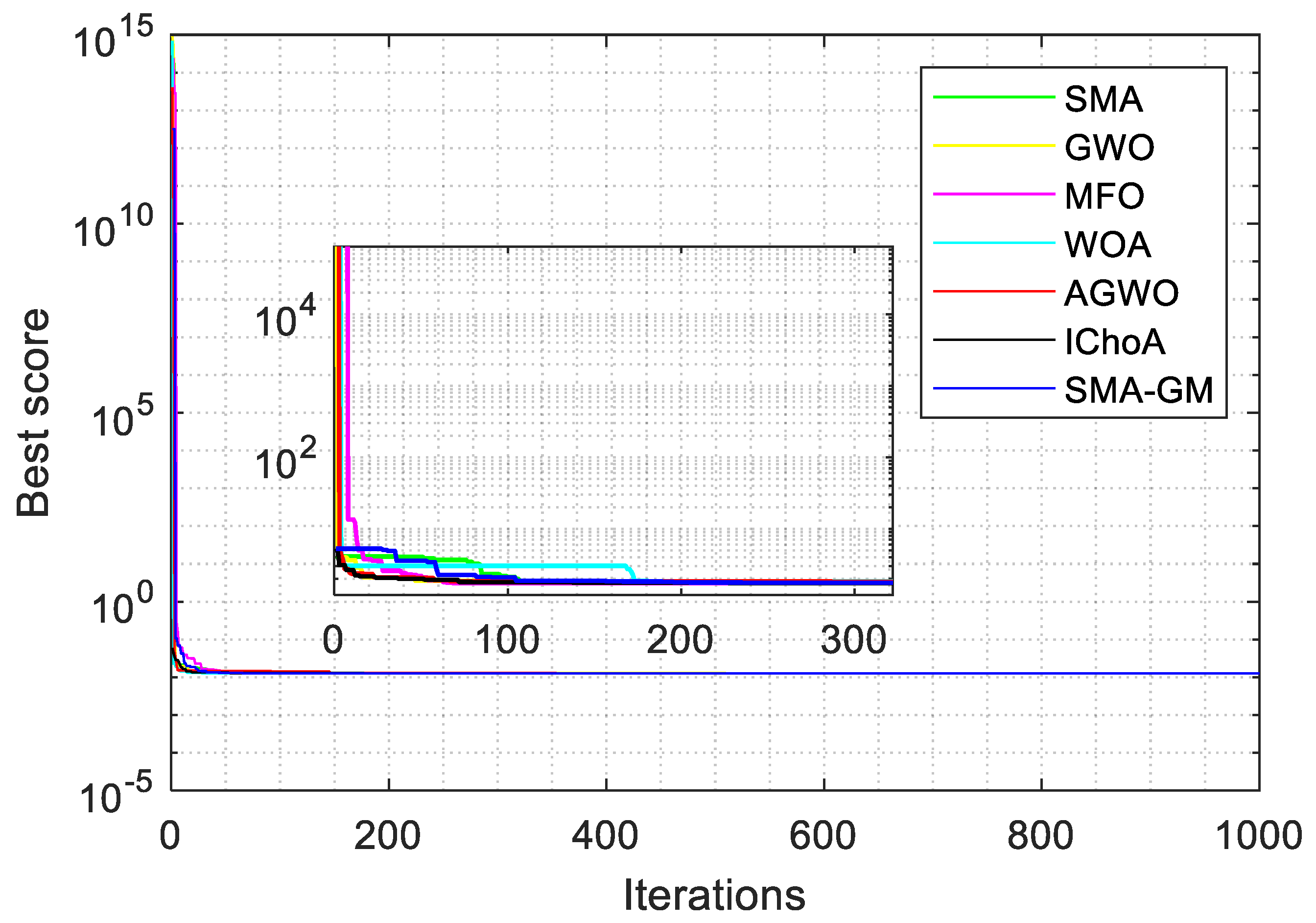
The optimal solution of SMA-GM and other counterparts on the welded beam problem are presented in Table 13 and Table 14, which gives the corresponding constraint values of these algorithms for this problem. According to the comparative results, SMA-SM achieved optimum parameter values resulting in optimum cost function value 1.7249 with ideal parameter [0.20573, 3.4704, 9.037, 0.20573] for welded beam design problem. Figure 8 shows the convergence behavior of the SMA-GM and other algorithms for this problem.

Table 13.
Optimal result of the welded beam design problem.

Table 14.
Constraint values of the welded beam design problem.
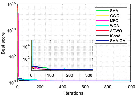
Figure 8.
Convergence curve for the welded beam design problem.
6.4. Tension/Compression Spring Design Problem
The tension/compression spring problem is a classic structural engineering design problem [33], whose purpose is to minimize the weight of tension or compression spring under certain constraints such as shear stress, surge frequency, and deflection. To solve the problem, three core variables are needed: the diameter of the wire (d), mean value of the coil diameter (D), and number of active coils (N). The mathematical model of this problem is as follows:
- Consider
The results of SMA-GM and competitor algorithms in terms of achieving the optimal solution for the tension/compression spring design optimization problem are reported in Table 15. In addition, Table 16 provides the corresponding constraint values of these algorithms for this problem. As can be seen from Table 15, the SMA-GM algorithm not only performed the best out of all comparison algorithms but also obtained the solution closest to the optimal value of the tension/compression spring design problem. For qualitative analysis, the convergence plots were recorded and illustrated in Figure 9 and the figure simply proves the efficient convergence potential of the SMA-GM. Therefore, we can say that the SMA-GM algorithm not only has an excellent ability to solve complex engineering problems but also shows high efficiency and accuracy and obtains the optimal solution with the best parameter and constraint values.

Table 15.
Optimal result of the tension/compression spring design problem.

Table 16.
Constraint values of the tension/compression spring design problem.
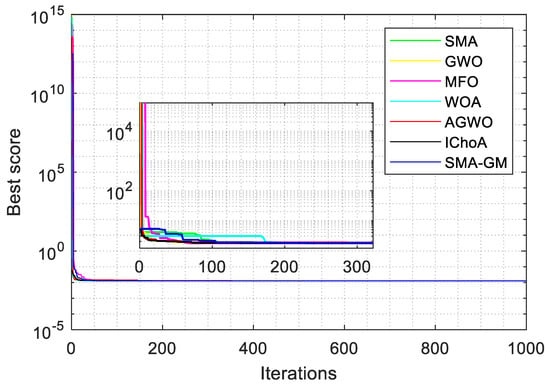
Figure 9.
Convergence curve for the tension/compression spring design problem.
7. Conclusions
A novel algorithm named SMA-GM has been proposed in this paper. SMA-GM has been proposed to address the shortcomings of the original SMA algorithm, such as its tendency to trap into local optima and insufficient exploitation. In the proposed method for avoiding SMA’s limitations, the exploitation phase of the original SMA has improved through the Gaussian mutation (GM) mechanism. The proposed SMA-GM performs exceptionally well in terms of convergence rate, stability, and optimization reliability compared to other metaheuristic algorithms. According to experiments conducted on the unconstrained, constrained, and CEC2022 functions and to further check the potential of SMA-GM, the complex constrained engineering problems show the superiority of the proposed algorithm as compared to other algorithms. To avoid the local optima, the GM strategy introduces a slight arbitrary variation into the group of search agents, improving convergence and enhancing exploitation potential while expanding the individual search space. Strengthening the global search and boosting the updated population is the primary goal of the proposed GM strategy. To guarantee that slime moulds with better fitness enter the next generation, the greedy selection mechanism was included. Convergence curves, diversity curves, and boxplot results showed that the proposed SMA-GM algorithm has efficiently enhanced the convergence accuracy, fitness performance, and the algorithm’s stability.
The proposed SMA-GM has some limitations in practical application. If the scale of the problem is too large, difficulty could arise in selecting the optimal solution. However, like other stochastic algorithms, SMA-GM might not always reach the global optima for all benchmark functions and is susceptible to being trapped at local minima. The limitations of SMA-GM must be addressed to improve its ability to provide global solutions. By overcoming these challenges, SMA-GM can advance toward becoming a widely accepted and widely used state-of-the-art algorithm.
In future studies, more effective constraint processing methods must be developed and incorporated into other metaheuristic algorithms. Multi-objective optimization is also a highly challenging area. Future work can focus on combining the proposed algorithm with different techniques to handle multi-objective optimization problems, focusing more on the operators to analyze the diversity and striking a balance between exploration and exploitation. Consequently, the proposed algorithm can be applied to complex optimization problems involving many design variables. It is worthwhile to investigate whether the SMA-GM may be used for a more extensive variety of real-life problems in future research. This will contribute to further validating the algorithm’s applicability to generate optimal solutions for a wide variety of optimization problems.
Author Contributions
G.T.: Conceptualization and Writing—original Draft, A.P.: Writing—review and editing and Supervision, N.M.: Methodology and Investigation, A.R.: Writing—review and editing, R.S.: Methodology, Supervision, Visualization, Writing—review and editing, Project Administration, and Funding Acquisition. All authors have read and agreed to the published version of the manuscript.
Funding
This research received no external funding.
Data Availability Statement
The data used in the current study are available from the corresponding author on reasonable request.
Conflicts of Interest
The authors declare no conflicts of interest regarding the publication of this research.
References
- Eberhart, R.; Kennedy, J. A new optimizer using particle swarm theory. In MHS’95, Proceedings of the Sixth International Symposium on Micro Machine and Human Science, Nagoya, Japan, 4–6 October 1995; IEEE: Piscataway, NJ, USA, 1995; pp. 39–43. [Google Scholar]
- Holland, J.H. Genetic algorithms. Sci. Am. 1992, 267, 66–73. [Google Scholar] [CrossRef]
- Mirjalili, S. Moth-flame optimization algorithm: A novel nature-inspired heuristic paradigm. Knowl. Based Syst. 2015, 89, 228–249. [Google Scholar] [CrossRef]
- Mirjalili, S.; Lewis, A. The Whale Optimization Algorithm. Adv. Eng. Softw. 2016, 95, 51–67. [Google Scholar] [CrossRef]
- Mirjalili, S.; Mirjalili, S.M.; Lewis, A. Grey Wolf Optimizer. Adv. Eng. Softw. 2014, 69, 46–61. [Google Scholar] [CrossRef]
- Wolpert, D.H.; Macready, W.G. No Free Lunch Theorems for Optimization. IEEE Trans. Evol. Comput. 1997, 1, 67–82. [Google Scholar] [CrossRef]
- Mirrashid, M.; Naderpour, H. Transit search: An optimization algorithm based on exoplanet exploration. Results Control Optim. 2022, 7, 100127. [Google Scholar] [CrossRef]
- Schlüter, M.; Gerdts, M. The oracle penalty method. J. Glob. Optim. 2010, 47, 293–325. [Google Scholar] [CrossRef]
- Li, S.; Chen, H.; Wang, M.; Heidari, A.A.; Mirjalili, S. Slime Mould Algorithm: A new method for stochastic optimization. Future Gener. Comput. Syst. 2020, 111, 300–323. [Google Scholar] [CrossRef]
- Yuan, L.; Ji, J.; Liu, X.; Liu, T.; Chen, H.; Chen, D. An Improved Elite Slime Mould Algorithm for Engineering Design. CMES-Comput. Model. Eng. Sci. 2023, 137, 415–454. [Google Scholar] [CrossRef]
- Naik, M.K.; Panda, R.; Abraham, A. An entropy minimization based multilevel colour thresholding technique for analysis of breast thermograms using equilibrium slime mould algorithm. Appl. Soft Comput. 2021, 113, 107955. [Google Scholar] [CrossRef]
- Houssein, E.H.; Mahdy, M.A.; Blondin, M.J.; Shebl, D.; Mohamed, W.M. Hybrid slime mould algorithm with adaptive guided differential evolution algorithm for combinatorial and global optimization problems. Expert Syst. Appl. 2021, 174, 114689. [Google Scholar] [CrossRef]
- Yu, C.; Heidari, A.A.; Xue, X.; Zhang, L.; Chen, H.; Chen, W. Boosting quantum rotation gate embedded slime mould algorithm. Expert Syst. Appl. 2021, 181, 115082. [Google Scholar] [CrossRef]
- Chauhan, S.; Vashishtha, G.; Kumar, A. A symbiosis of arithmetic optimizer with slime mould algorithm for improving global optimization and conventional design problem. J. Supercomput. 2022, 78, 6234–6274. [Google Scholar] [CrossRef]
- Juan, Z.; Zheng-Ming, G.; Wu, S. The improved slime mould algorithm with Levy flight. J. Phys. Conf. Ser. 2020, 1617, 012033. [Google Scholar]
- Abualigah, L.; Diabat, A.; Elaziz, M.A. Improved slime mould algorithm by opposition-based learning and Levy flight distribution for global optimization and advances in real-world engineering problems. J. Ambient. Intell. Humaniz. Comput. 2023, 14, 1163–1202. [Google Scholar] [CrossRef]
- Örnek, B.N.; Aydemir, S.B.; Düzenli, T.; Özak, B. A novel version of slime mould algorithm for global optimization and realworld engineering problems: Enhanced slime mould algorithm. Math. Comput. Simul. 2022, 198, 253–288. [Google Scholar] [CrossRef]
- Yu, C.; Cai, Z.; Ye, X.; Wang, M.; Zhao, X.; Liang, G.; Li, C. Quantum-like mutation-induced dragonfly-inspired optimization approach. Math. Comput. Simul. 2020, 178, 259–289. [Google Scholar] [CrossRef]
- Zhang, X.; Xu, Y.; Yu, C.; Heidari, A.A.; Li, S.; Chen, H.; Li, C. Gaussian mutational chaotic fruit fly-built optimization and feature selection. Expert Syst. Appl. 2020, 141, 112976. [Google Scholar] [CrossRef]
- Chen, H.; Zhang, Q.; Luo, J.; Xu, Y.; Zhang, X. An enhanced bacterial foraging optimization and its application for training kernel extreme learning machine. Appl. Soft Comput. 2020, 86, 105884. [Google Scholar] [CrossRef]
- Luo, J.; Chen, H.; Xu, Y.; Huang, H.; Zhao, X. An improved grasshopper optimization algorithm with application to financial stress prediction. Appl. Math. Model. 2018, 64, 654–668. [Google Scholar] [CrossRef]
- Wu, S.; Heidari, A.A.; Zhang, S.; Kuang, F.; Chen, H. Gaussian bare-bone slime mould algorithm: Performance optimization and case studies on truss structures. Artif. Intell. Rev. 2023, 56, 9051–9087. [Google Scholar] [CrossRef]
- Bäck, T.; Schwefel, H.P. An overview of evolutionary algorithms for parameter optimization. Evol. Comput. 1993, 1, 1–23. [Google Scholar] [CrossRef]
- Ma, C.; Huang, H.; Fan, Q.; Wei, J.; Du, Y.; Gao, W. Grey wolf optimizer based on Aquila exploration method. Expert Syst. Appl. 2022, 205, 117629. [Google Scholar] [CrossRef]
- Preeti; Kaur, R.; Singh, D. Dimension learning based chimp optimizer for energy efficient wireless sensor networks. Sci. Rep. 2022, 12, 14968. [Google Scholar] [CrossRef] [PubMed]
- Qtaish, A.; Albashish, D.; Braik, M.; Alshammari, M.T.; Alreshidi, A.; Alreshidi, E.J. Memory-based Sand Cat Swarm Optimization for Feature Selection in Medical Diagnosis. Electronics 2023, 12, 2042. [Google Scholar] [CrossRef]
- Duan, Y.; Liu, C.; Li, S.; Guo, X.; Yang, C. Manta ray foraging and Gaussian mutation-based elephant herding optimization for global optimization. Eng. Comput. 2023, 39, 1085–1125. [Google Scholar] [CrossRef]
- Deb, K. An efficient constraint handling method for genetic algorithms. Comput. Methods Appl. Mech. Eng. 2000, 186, 311–338. [Google Scholar] [CrossRef]
- Runarsson, T.P.; Yao, X. Stochastic ranking for constrained evolutionary optimization. IEEE Trans. Evol. Comput. 2000, 4, 284–294. [Google Scholar] [CrossRef]
- Abdel-Basset, M.; Mohamed, R.; Sallam, K.M.; Chakrabortty, R.K. Light spectrum optimizer: A novel physics-inspired metaheuristic optimization algorithm. Mathematics 2022, 10, 3466. [Google Scholar] [CrossRef]
- Derrac, J.; García, S.; Molina, D.; Herrera, F. A practical tutorial on the use of nonparametric statistical tests as a methodology for comparing evolutionary and swarm intelligence algorithms. Swarm Evol. Comput. 2011, 1, 3–18. [Google Scholar] [CrossRef]
- Azizi, M.; Talatahari, S.; Giaralis, A. Optimization of engineering design problems using atomic orbital search algorithm. IEEE Access 2021, 9, 102497–102519. [Google Scholar] [CrossRef]
- Kumar, A.; Wu, G.; Ali, M.Z.; Mallipeddi, R.; Suganthan, P.N.; Das, S. A test-suite of non-convex constrained optimization problems from the real-world and some baseline results. Swarm Evol. Comput. 2020, 56, 100693. [Google Scholar] [CrossRef]
Disclaimer/Publisher’s Note: The statements, opinions and data contained in all publications are solely those of the individual author(s) and contributor(s) and not of MDPI and/or the editor(s). MDPI and/or the editor(s) disclaim responsibility for any injury to people or property resulting from any ideas, methods, instructions or products referred to in the content. |
© 2024 by the authors. Licensee MDPI, Basel, Switzerland. This article is an open access article distributed under the terms and conditions of the Creative Commons Attribution (CC BY) license (https://creativecommons.org/licenses/by/4.0/).


