Music Genre Classification Based on VMD-IWOA-XGBOOST

Abstract

Music genre classification is significant to users and digital platforms. To enhance the classification accuracy, this study proposes a hybrid model based on VMD-IWOA-XGBOOST for music genre classification. First, the audio signals are transformed into numerical or symbolic data, and the crucial features are selected using the maximal information coefficient (MIC) method. Second, an improved whale optimization algorithm (IWOA) is proposed for parameter optimization. Third, the inner patterns of these selected features are extracted by IWOA-optimized variational mode decomposition (VMD). Lastly, all features are put into the IWOA-optimized extreme gradient boosting (XGBOOST) classifier. To verify the effectiveness of the proposed model, two open music datasets are used, i.e., GTZAN and Bangla. The experimental results illustrate that the proposed hybrid model achieves better performance than the other models in terms of five evaluation criteria.

1. Introduction

Mobile devices and streaming services have revolutionized music access, making it more convenient for users. The abundance of digital music poses a significant challenge for music information retrieval (MIR), particularly in swiftly locating preferred tracks within vast libraries based on genres. Music genre classification (MGC) is a popular application for MIR, and music genres are vital labels for organizing and retrieving music, which is essential for solving classification challenges [1,2].

Most of the early music genre classification and labeling was performed manually, which required worker expertise. Music streaming platforms often employ music specialists to conduct music tagging, leading to high accuracy, albeit at a substantial expense. At times, platforms permit non-professional users to contribute tags by making the tagging feature accessible, and these user-generated tagging data are incorporated into the music tags. While this approach reduces costs, it often results in numerous instances of mislabeling within categories [3]. Therefore, it is necessary to achieve music genre classification by computational methods. Currently, the mainstream classification of music genres is divided into two classification methods: image classification, based on music spectrograms, and symbolic description music classification, based on symbolic data types [4].

For the first classification method, most studies perform the short-time Fourier transform (STFT) on the raw data, visualizing the raw data as spectrograms, or obtain Meier spectrograms so as to acquire deeper acoustic features to improve the classification accuracy of the subsequent model. With the breakthrough of computer vision (CV), researchers have carried out a series of studies on music genre classification based on deep learning (DL) [5]. Since the spectrogram of audio is similar to that of red-green-blue (RGB) images, most CV models can be applied in the field of MGC. In view of this, Oliveira et al. [6] transformed audio signals into spectrograms and extracted features from images. Yang et al. [7] proposed a novel method for music genre classification that can be applied to the spectrograms. By considering the possible differences between spectra, he proposed an attention mechanism model based on the bidirectional recurrent neural network (BRNN) for music genre classification, and experiments showed that the proposed model outperformed the traditional model. Cheng et al. [8] combined the music genre classification with the YOLO architecture. In their work, extracted visual Meier spectrograms were used as the input features, and higher accuracy was achieved. Laiali et al. [9] transformed audio data into spectrograms using STFT, the audio features were extracted using Mel-frequency cepstral coefficients (MFCCs) for classification, and the experimental results showed that AlexNet demonstrated the best performance among the group of convolutional neural network (CNN) classifiers. Costa et al. [10] proposed a novel method to transform audio signals into spectrograms and extract texture features from image time-frequency features; this method surpassed the best results in the MIREX2010 competition in the LMD dataset. Gan [11] found that the CNN-based method ignores the temporal characteristics of the audio itself; therefore, he combined the convolutional structure with a bidirectional recurrent neural network and proposed a convolutional recurrent neural network classification architecture. Accurate results on the GTZAN dataset were obtained. Balachandra [12] improved the moth algorithm IMOF and successfully applied it to the task of music genre classification. He achieved good classification results by optimizing the weights of a deep belief network (DBN) and performing classification. Wang et al. [13] used bidirectional long short-term memory (BiLSTM) for feature extraction and VGG-16Net to achieve better results on the MSD-I, GTZAN, and ISMIR2004 datasets. Rui [14] found that manual parameter setting could not achieve good results in music emotion classification. Therefore, Rui proposed the quantum particle swarm optimization (QPSO) algorithm to optimize the parameters of the CNN-RF model. Li et al. [15] found that a traditional CNN attempts to classify the input spectrograms with a softmax layer that lacks the ability to distinguish the deeper features of the music. In response to inadequate discrimination caused by softmax loss, an angular margin and cosine margin softmax loss (AMCM-Softmax) approach is proposed to augment the discriminative efficacy of deep features.

For the second classification method, as these music features are rooted in musical symbols, prevalent formats such as Music Digital Interface (MIDI), MusicXML, and MEI are frequently utilized [16]. In order to capture more features when performing classification, some scholars began to use symbolic data types. For example, as early as 2003, Tzanetakis and Cook used a duration histogram (DH) to capture rhythmic information for classification, and, at the same time, they established one of the most widely used publicly available datasets, GTZAN [17]. Karydis captured the pitch information characteristics of music to classify genres and achieved good performance [18]. In 2004, McKay and Fujinaga extracted 109 high-level musical features from MIDI files, which are related to the strength, instrumentation, pitch, melody, rhythm, and chords of music. The number of features was expanded in the literature [19] to 160, which were used to automatically classify music genres; good classification results were obtained. Jorge et al. [20] incorporated conventional musical attributes, such as note histograms and statistical moments, alongside innovative features extracted from MIDI files to classify genres using a traditional machine learning classifier. Their findings indicate that regular-kNN surpasses other traditional machine learning models in performance. Lee et al. [21] expanded their analysis by incorporating additional musicological features, blending musical instrument data with raw audio and MIDI phrases as input variables for classification. They employed traditional machine learning algorithms, such as support vector machines (SVM), decision trees, and random forest (RF), for their classification tasks. Qiu et al. [22] introduced an unsupervised latent music representation learning method based on a deep 3D convolutional denoising autoencoder (3D-DCDAE) for music genre classification. This method aims to learn common representations from a large amount of unlabeled data to improve the performance of music genre classification. This not only minimizes training time compared to partial models but also achieves superior classification accuracy. Cheng et al. [23] used Librosa to classify raw audio by measuring its key features such as the corresponding Mel-spectrum, which greatly improved the convenience of feature extraction. Meanwhile, Sakinat O. et al. [24] utilized publicly available Nigerian songs to extract audio features using Librosa. They introduced the ORIN dataset, making it publicly accessible. In addition, kNN, SVM, extreme gradient boosting (XGBOOST), and RF were employed. Experimental results revealed that XGBOOST outperformed other methods, achieving superior classification accuracy.

Given the above analysis, the existing studies achieved competitive performance in music genre classification. However, some issues still need to be addressed: (i) In terms of feature extraction, various feature selection algorithms are used to capture the powerful features, but the intrinsic pattern of original features can be further extracted. (ii) Regarding parameter optimization, machine learning models rely on the parameter setting in classification tasks, but traditional parameter optimization methods (such as grid search, PSO algorithm, etc.) always obtain a local optimization solution, resulting in limited performance.

In view of this, this paper introduces a hybrid model for music genre classification. The original audio is transformed into numerical data first; then, the maximum information coefficient (MIC) is used for feature selection. Subsequently, variational mode decomposition (VMD) is employed to extract the inner pattern of the top-five features. To reduce the complexity and capture effective information from original features, in this paper, we adopt the decomposition-based approach for classification. The main contributions are outlined as follows:

• A hybrid model with VMD-IWOA-XGBOOST is proposed for music genre classification. MIC is used to screen out high-correlation features, VMD is chosen to extract the key information of features, an Improved Whale Optimization Algorithm (IWOA) is proposed to improve the parameter setting, and XGBOOST is utilized as the classification model.
• An IWOA is proposed for parameter optimization. By refining the search process, contracting encircling, and altering the spiral position, comparative analysis reveals the superiority of the IWOA.

The remainder of the paper is organized as follows: Section 2 describes the methodology; Section 3 describes the experimental results and analytics; Section 4 summarizes the conclusions.

2. Methodology

2.1. Feature Extraction

In this paper, we extract features from time and frequency domains for the GTZAN dataset, and the following main musical features have a large difference in classification of musical genres: zero-crossing rate (ZCR), spectral centroid, spectral roll-off, spectral bandwidth, chroma frequency, root-mean-square energy (RMSE), delta, Mel-spectrogram, tempo, and Mel-frequency cepstral coefficients (MFCCs) [25]. Below, we provide descriptions of features extracted from the frequency domain:

(1)

The zero-crossing rate is the rate of change of a signal symbol, i.e., the probability of changing from a negative or opposite number to a positive number [26]. The over-zero rate is an important feature in the field of speech recognition and music information retrieval, and its defining formula is provided below:

$$zcr=\frac{1}{T-1}{\displaystyle \sum _{t=1}^{T-1}sign\left\{s_t{s}_{t-1}<0\right\}}$$

(1)

where $s$ is the signal length $T$, and the $sign$ function assigns a value of 1 when {} is true, and 0 otherwise.

(2)

The spectral center of mass is a critical physical parameter elucidating the timbral characteristics of a sound signal. It delineates the frequency-weighted average of energy distribution within a specified frequency band, functioning as the locus of gravity for its constituent frequencies. Consequently, it offers pivotal insights into the frequency and energy distributions inherent to the sound signal. It represents the brightness of the signal spectrum and is regarded as the cross-section of the STFT amplitude spectrum. The following is its defining formula:

$$sc=\frac{{\displaystyle \sum _{k=1}^{K}kX\left(k\right)}}{{\displaystyle \sum _{k=1}^{K}X\left(k\right)}}$$

(2)

where $X\left(k\right)$ is the spectrum of the DFT (discrete Fourier transform) at moment $k$ of amplitude.

(3)

Spectral roll-off generally means that the frame center frequency is below the default threshold of the spectrum (typically 85%). This is another attribute used to estimate the spectral pattern. Spectral roll-off points serve as discriminative indicators within audio signals, facilitating the identification of distinct sounds, including the timbral nuances exhibited by various instruments. These features, typically integrated with other descriptors such as MFCCs, zero-crossing rate, and bandwidth measures, are employed synergistically to enhance the efficacy of audio processing tasks. The calculation formula is provided below:

$${\displaystyle \sum _{n=1}^{Q_t}0.85\times X\left(k\right)}$$

(3)

(4)

Spectral bandwidth refers to a fundamental parameter in signal processing and spectroscopy, representing the range of frequencies encompassed by a signal or a spectral distribution. It is calculated with the following formula:

$$f_c=\frac{{\displaystyle \sum _{k=1}^K}s\left(k\right)f\left(k\right)}{{\displaystyle \sum _{k=1}^K}s\left(k\right)}$$

(4)

(5)

Chroma frequency is used to indicate the energy of each tone level between musical signals, providing a metric characteristic in cases where there is a great similarity between musical segments.

(6)

RMSE is a method of characterizing the energy of a signal. It is expressed in Equation (5), while its rooted calculation is shown in Equation (6).

$${\displaystyle \sum _{n=1}^N{\left|x\left(n\right)\right|}^2}$$

(5)

where $x\left(n\right)$ denotes the discrete time node signal.

$$\sqrt{\frac{{\displaystyle \sum _{n=1}^N}{\left|x\left(n\right)\right|}^2}{N}}$$

(6)

(7)

In the case of Mel-frequency cepstral coefficients (MFCCs), the vast majority of its parameters are related to the amplitude of the frequency. The MFCC is an important feature of audio signals and it is used for rapid speech recognition [27]. Its equation is as follows:

$$mel\left(f\right)=1125\times \ln \left(1+\frac{f}{100}\right)$$

(7)

(8)

The harmonic and percussive harmonic will reveal more horizontal or pitch-dependent changes. The percussive harmonic will show more vertical or time-dependent changes. These features are generally obtained using a fast Fourier transform (FFT).

(9)

Tempo is a fundamental aspect of music theory and analysis, denoting the rate or speed at which a musical piece progresses, typically measured in beats per minute (BPM).

2.2. The Maximal Information Coefficient

Reshef et al. proposed the maximum information coefficient, which can not only measure the linear and nonlinear relationship between data variables but can also mine the non-functional dependence between variables [28].

The calculation of MIC is very simple; if there exist two variables $V_1$ = {$v_1\left(i\right)$ }, $i$ = 1, 2, …, $n$ and $V_2$ = {$v_2\left(i\right)$ }, $i$ = 1, 2, …, n, both of which are related in some way, and if those variables $v_1\left(i\right)$ and $v_2\left(i\right)$, $i$ = 1, 2, …, n, can be formed into a set $D$ {$v_1\left(i\right)$, $v_2\left(i\right)$ }, then the calculation for determining the relationship between the two sides of the above is as follows:

(1)

Firstly, $V_1$ and $V_2$ are arranged in ascending order, and, subsequently, an $x_t$ × $y_t$ grid $G_t$ is defined as a sequence partition, where each sample point of $V_1$ is partitioned into $x_t$ parts, each sample point of $V_2$ is partitioned into $y_t$ parts, and some cells are allowed to be empty sets.

(2)

The probability distribution function $D{|}_{G_t}$ of all cells of the grid $G_t$ species is derived; at this time, the maximum mutual information value obtained is $\max$ $I\left(D{|}_{G_t}\right)$, and the value of its identity matrix is $M{\left(D\right)}_{x,y}$, as shown in Equation (8):

$$M{\left(D\right)}_{x,y}=\frac{\max I\left({D|}_{G_i}\right)}{\ln \min \left(x,y\right)}=\frac{p\left(x_t,y_t\right)\ln \frac{p\left(x_t,y_t\right)}{p\left(x_t\right)p\left(y_t\right)}}{\ln \min \left(x_t,y_t\right)}=\frac{\max \left({\displaystyle \sum _{i=1}^x}{\displaystyle \sum _{j=1}^y}\ln \frac{n_{ij}}{N}-{\displaystyle \sum _{i=1}^x}\frac{{\displaystyle \sum _{j=1}^y}{n}_{ij}}{N}\ln \frac{{\displaystyle \sum _{j=1}^y}{n}_{ij}}{N}-{\displaystyle \sum _{i=1}^y}\frac{{\displaystyle \sum _{j=1}^x}{n}_{ij}}{N}\ln \frac{{\displaystyle \sum _{j=1}^x}{n}_{ij}}{N}\right)}{\ln \min \left(x_t,y_t\right)}$$

(8)

where $p\left(x_t,y_t\right)$ represents the joint probability density function of elements $x_t$ and $y_t$ within grid $G_t$. $p\left(x_t\right)$ and $p\left(y_t\right)$ denotes the edge density distribution functions of $x_t$ and $y_t$, respectively. $n_{ij}$ is the number of cell samples falling in the $j$ th row and the $i$ th column of the grid $G$, and $N$ is the total number of samples.

(3)

Since different grids $G$ lead to different probability distribution functions D|G, the maximum mutual information coefficients MIC of the variables $V_1$ and $V_2$ are searched for the optimal grid $G$ by the exhaustive method for the feature matrix:

$$MIC\left(D\right)=\underset{xy<B\left(N\right)}{\max }\left\{M{\left(D\right)}_{x,y}\right\}=\max \frac{\max I\left({D|}_G\right)}{\ln \min \left(x,y\right)}=M\left(D\right)x,y$$

(9)

where $I\left(D{|}_G\right)$ represents the probability distribution function encompassing all elements within the grid $G_t$. $B\left(N\right)$ is the maximum grid for an exhaustive search.

The final MIC obtained is assigned values between [0, 1]; the greater the correlation of the variables, the greater the MIC value, and vice versa.

2.3. Variational Mode Decomposition

VMD is a non-recursive signal processing method which can decompose the original signal f(t) into a series of intrinsic mode function (IMF) with finite bandwidth by iteratively searching for the optimal solution of the variational modes. The method has good noise immunity and can effectively overcome the mode aliasing problem of empirical mode decomposition (EMD) [29]. The essential idea of VMD is to computationally solve the variational problem. The computational steps are as follows:

(1)

The analytical signal of each mode is solved by the Hilbert transform, and the spectrum is constructed at the same time. Finally, the analytical signal of each decomposed mode component $u_k$ at time t is obtained:

$$\left(\delta \left(t\right)+\frac{j}{\pi t}\right)\times u_k\left(t\right)$$

(10)

(2)

The predicted center frequency is multiplied with the resolved signal of each IMF component for frequency correction, and the spectrum of each decomposed IMF component is shifted to the corresponding frequency band:

$$\left[\left(\delta \left(t\right)+\frac{j}{\pi t}\right)\times u_k\left(t\right)\right]e^{-j{\omega }_{k}t}$$

(11)

where $\left(\delta \left(t\right)+\frac{j}{\pi t}\right)$ is the Hilbert transform functor and $e^{-j{\omega }_{k}t}$ is the correction factor.

(3)

The variational problem with constraints is constructed by using the above-demodulated signal, calculating the bias, and then estimating the bandwidth from its squared paradigm, as shown below:

$$\left\{\begin{array}{l}\underset{\left\{u_k\hspace{1em}{\omega }_k\right\}}{\min }\left\{{\displaystyle \sum _{k=1}^K{\left|{\partial }_t\left[\left(\delta \left(t\right)+\frac{j}{\pi t}\right)\times u_k\left(t\right)\right]e^{-j{\omega }_{k}t}\right|}_2^2}\right\}\hfill \\ s.t.{\displaystyle \sum _{k=1}^K{u}_k\left(t\right)=f\left(t\right)}\hfill \end{array}\right.$$

(12)

where $\left\{u_k\right\}$ is the set of IMF components for each decomposition, $\left\{w_k\right\}$ denotes the set of center frequencies for each mode component, ${\partial }_t$ denotes the bias operation on the variable t, $\delta \left(t\right)$ denotes the unit-pulse signal function, * denotes the convolution operation, $f\left(t\right)$ denotes the original signal, and ${\left| \right|}_2^2$ denotes the L2 paradigm.

(4)

In order to transform the constrained variational problem into an $\alpha$ variational problem without constraints, the original problem can be converted into a problem of solving the Lagrange function maximum by introducing the Lagrange multiplier a with the quadratic penalty factor $\lambda$, which has the following expression:

$$L\left(\left\{{\mu }_k\right\},\left\{{\omega }_k\right\},\alpha \right)=\alpha {\displaystyle \sum _{k=1}^K\left|{\left.{\partial }_t\left[\left(\delta \left(t\right)+\frac{j}{\pi t}\right)\times u_k\left(t\right)\right]e^{-j{\omega }_{k}t}\right|}_2^2\right.}+{\left|\left.f\left(t\right)-{\displaystyle \sum _{k=1}^K{u}_k\left(t\right)}\right|\right.}_2^2+<\alpha \left(t\right),f\left(t\right)-{\displaystyle \sum _{k=1}^K{u}_k\left(t\right)} >$$

(13)

where $\alpha$ denotes the Lagrange multiplier, $\lambda$ denotes the quadratic penalty factor, and $< , >$ denotes the dot product operation.

(5)

The optimal solution of the constrained variational model is solved by updating $u_k$, $w_k$, and $\alpha$ in the frequency domain using the alternating direction multiplier method, and the updated equation is shown below:

$${\widehat{\mu }}_k^{n+1}\left(\omega \right)=\frac{\widehat{f}\left(\omega \right)-{\displaystyle \sum _{i\ne k}{\widehat{\mu }}_i\left(\omega \right)+\frac{\widehat{\alpha }\left(\omega \right)}{2}}}{1+2\lambda {\left(\omega -{\omega }_k\right)}^2}$$

(14)

$${\omega }_k^{n+1}=\frac{{\displaystyle {\int }_0^{\infty }\omega {\left|\left.{{\widehat{\mu }}_k}^{n+1}\left(\omega \right)\right|\right.}_2^2}d\omega }{{\displaystyle {\int }_0^{\infty }\left|{\left.{{\widehat{\mu }}_k}^{n+1}\left(\omega \right)\right|}_2^{2}d\omega \right.}}$$

(15)

$${\alpha }^{n+1}\left(\omega \right)={\alpha }^n\left(\omega \right)+\Theta \left[\widehat{f}\left(\omega \right)-{\displaystyle \sum _{k=1}^K{{\widehat{\mu }}_k}^{n+1}\left(\omega \right)}\right]$$

(16)

$${\displaystyle \sum _{k=1}^K\frac{\Vert {{\widehat{\mu }}_k}^{n+1}\left(\omega \right)-{{\widehat{\mu }}_k}^n\left(\omega \right){\Vert }_2^2}{\Vert {{\widehat{\mu }}_k}^{n+1}\left(\omega \right){\Vert }_2^2}}<\epsilon$$

(17)

where $n$ is the number of iterations; ${\widehat{\mu }}_i\left(\omega \right)$,$\widehat{f}\left(\omega \right)$, and $\widehat{\alpha }\left(\omega \right)$ are the Fourier transforms of $\mu \left(t\right)$, $f\left(t\right)$, and $\alpha \left(t\right)$, respectively; $\left|{\widehat{\mu }}_k\left(\omega \right)\right|$ is the Wiener filtering of each component of IMF after Fourier transform; $\Theta$ is the noise tolerance limit; ${{\omega }_k}^{n+1}$ is the center frequency of the $k$ th mode component at the $n+1$ th iteration; and $\epsilon$ is the set threshold of convergence accuracy. Using Equations (12)–(14), ${{\mu }_k}^{n+1}$, ${{\omega }_k}^{n+1}$, and ${\alpha }^{n+1}$ are continuously updated until the termination condition of Equation (17) is satisfied; then, the iteration is terminated.

2.4. Improved Whale Optimization Algorithm

The WOA algorithm is a bionic intelligent optimization algorithm that has been developed to simulate the unique foraging style of whales. It assumes that the current individual is the prey, and all other individuals in the group approach the optimal individual. The WOA is divided into three main phases: searching for foraging, contraction of encirclement, and helical updating of the position [30]. The underlying WOA formula can be found in the literature [30]. This study proposes an improved whale optimization algorithm, as described below.

(1)

Adaptive weighting

First, we choose the number of iterations t to constitute the adaptive inertia weights, as shown in Equation (18), based on the variation of the number of update iterations in the whale optimization algorithm:

$$w\left(t\right)=0.2\times \cos \left(\frac{\pi }{2}\times \left(1-\frac{t}{t_{\max }}\right)\right)$$

(18)

The improved whale optimization algorithm position is updated as follows:

$$\overrightarrow{X}\left(t+1\right)=\left\{\begin{array}{ll}w\left(t\right){\overrightarrow{X}}^{\ast }\left(t\right)-\overrightarrow{A}\cdot \overrightarrow{D}\hfill & ,if p<0.5\\ w\left(t\right)\overrightarrow{X^{\ast }}+\overrightarrow{D^{\prime }}\times e^{bl}\times \cos \left(2\pi l\right)\hfill & ,if p\ge 0.5\end{array}\right.$$

(19)

(2)

Variable helix position

The parameter b is designated as a variable that changes with the number of iterations to dynamically adjust the shape of the spiral during whale searching, and after combining the adaptive weights, the new spiral position is updated as follows:

$$\overrightarrow{X}\left(t+1\right)=\overrightarrow{D^{\prime }}\times e^{bl}\times \cos \left(2\pi l\right)+\overrightarrow{X^{\ast }}$$

(20)

$$b=e^{5\times \cos \left(\pi \times \left(1-\frac{t}{t_{\max }}\right)\right)}$$

(21)

(3)

Differential variance scale factor

We found that the algorithm will generate new feasible solutions around the optimal solution when it is close to the optimal solution, which will cause premature convergence as the number of iterations increases. To solve this problem, we borrowed the idea of variance perturbation factor for use in the differential evolutionary algorithm and introduced this variance perturbation factor in the process of shrinking the surroundings to form the optimal solution, which can make the algorithm jump out of the local optimum and improve the optimization accuracy of the local optimum [31]. The variance perturbation factor is shown in Equation (22):

$$\gamma =F\left({\overrightarrow{X}}^{\ast }\left(t\right)-\overrightarrow{X}\left(t\right)\right)$$

(22)

where $F$ is the variance perturbation factor.

2.5. XGBOOST

Extreme gradient boosting tree (GBDT) is an optimization of the boosting algorithm, which combines multiple regression tree classifiers into a single powerful classifier with the advantages of fast training speed with high generalization ability [32]. It generates new trees to fit the residuals of the previous tree by iterating continuously, and its accuracy improves as the number of iterations increases. The simplified form of its objective function after Taylor expansion is shown in (23):

$$O_{obj}=-\frac{1}{2}{\displaystyle \sum _{j=1}^T\frac{G_j^2}{H_j+\lambda }+}\gamma T$$

(23)

where $O_{obj}$ is the objective function, T is the number of leaves in the regression tree, $G_j$ is the first order derivative, $H_j$ is the second order derivative, $\lambda$ is the regularization parameter, and $\gamma$ is the learning rate.

2.6. The Proposed VMD-IWOA-XGBOOST Model

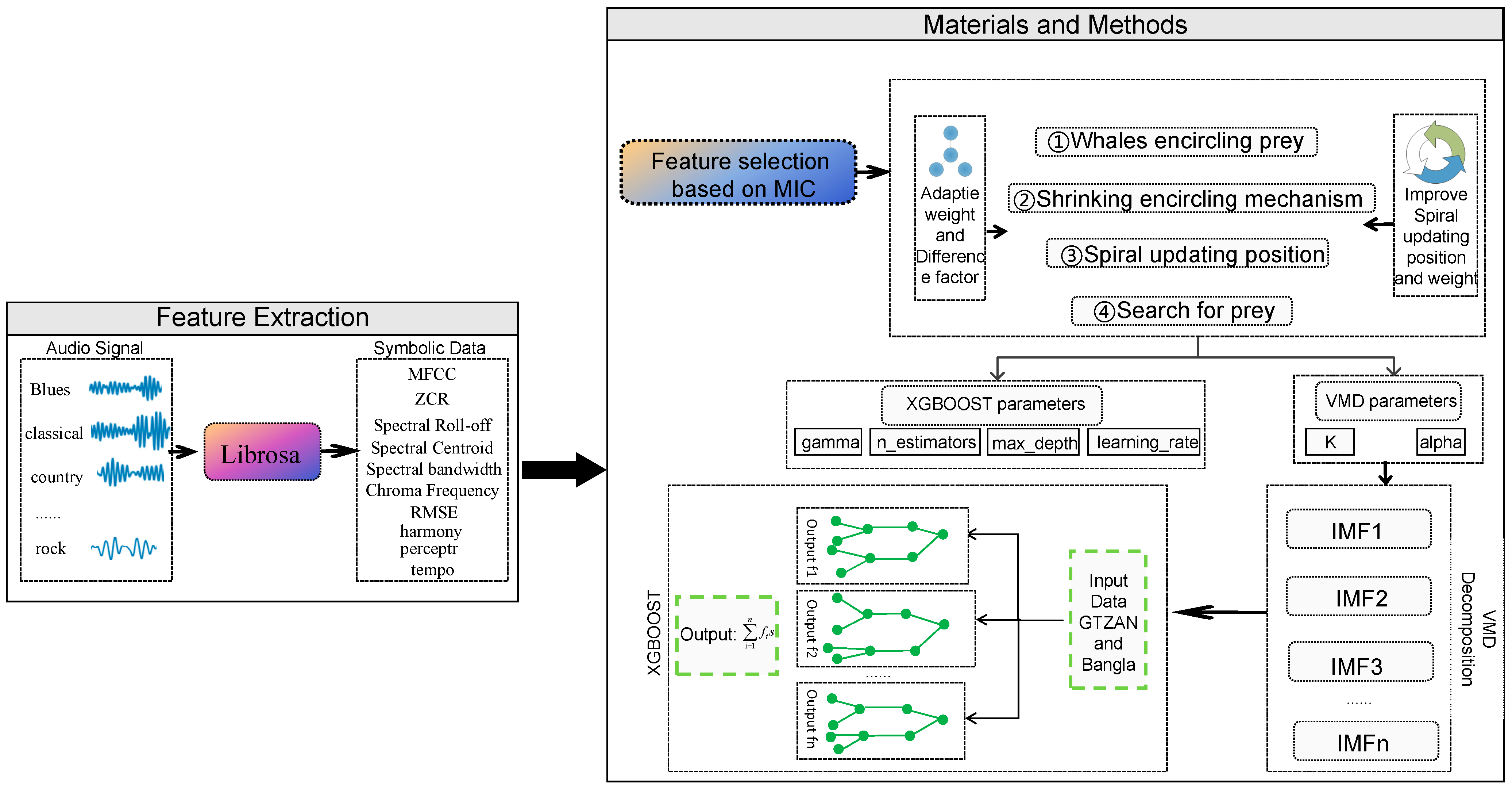
In this section, we describe the framework of the VMD-IWOA-XGBOOST model. The modeling framework is shown in Figure 1. The details are elaborated as follows:

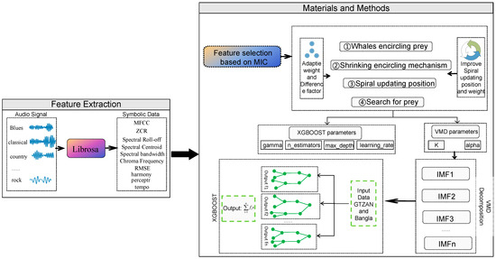
Figure 1. Music genre classification framework.

Step1: the original GTZAN audio dataset is processed through Librosa (version of Librosa is 0.9.1).

Step2: critical features are selected through MIC, the highest features are obtained first, and decomposition techniques are used to reduce the complexity of selected features.

Step3: we optimize the parameters of VMD and XGBOOST using the IWOA.

Step4: we carry out feature decomposition using the IWOA-optimized VMD method.

Step5: the decomposed modes are divided into a training set and a test set with 80% in the training set and 20% in the test set.

Step6: IWOA-optimized XGBOOST is used to classify.

3. Experiment

3.1. Data Set

We used two open datasets (GTZAN and Bangla) for the experiment. GTZAN is a classical dataset that includes a collection of 10 Western music genres, including but not limited to hip-hop, country, metal, blues, jazz, rock, disco, etc. Each of these genres contains 100 pieces of music, and each piece of music (a total of 1000 songs) is in a 30-s WAV audio format with 16-bit audio files in 22,050 HZ mono [24]. Considering the richness and diversity of Bangla music, we selected a Bangla music dataset for music genre classification, following the work of Mamun [26] et al., by selecting six classic Bangla music genres, each with approximately 250–300 songs of music. We named this the Bangla Music Dataset and made it available.

3.2. Evaluation Criteria

In order to verify the generalization of our proposed model, we employ the GTZAN and Bangla datasets. We adopted $macro-precision$, $macro-recall$, $macro-F1-score$, $Accuracy$, and $MCC$ to evaluate experimental results. Firstly, we introduced the basic $precision$, $recall$, $F1-score$, $Accuracy$ and $MCC$. Equation (24) is the $precision$ formula, $TP$ is the true example, and $FP$ is the false positive example. Precision can be interpreted as the ability of the classifier to predict only true samples as positive and actually correct. Equation (25) is the recall formula, $FN$ is the false negative example, and recall can be understood as the percentage of the number of test samples that are true positive examples that are actually classified as positive. Equation (26) is the formula for $F1-score$ calculation, and $F1$ is the harmonic mean coefficient between $precision$ and $recall$; if the $precision$ and $recall$ are higher, then the value of $F1$ will be higher. Equation (27) is the formula for $Accuracy$, $TN$ is the true counterexample, and the purpose of calculating $Accuracy$ is to find the ratio of the number of correct judgments to all judgments. In order to achieve a fairer experimental result, we will use $precision$, $recall$, and $F1-score$ to find their respective average values. The calculation formula is shown in Equations (28)–(30).

$$precision=\frac{TP}{TP+FP}$$

(24)

$$recall=\frac{TP}{TP+FN}$$

(25)

$$F1-score=\frac{2\times \left(precision\times recall\right)}{precision+recall}$$

(26)

$$Accuracy=\frac{TP+TN}{TP+FN+FP+FN}$$

(27)

$$MCC=\frac{TP\times TN-FP\times FN}{\sqrt{\left(TP+FP\right)\left(TP+FN\right)\left(TN+FP\right)\left(TN+FN\right)}}$$

(28)

$$macro-precision=\frac{1}{n}{\displaystyle \sum _{i=1}^{n}precision}$$

(29)

$$macro-recall=\frac{1}{n}{\displaystyle \sum _{i=1}^{n}recal{l}_i}$$

(30)

$$macro-F1=\frac{2\times \left(macro-precision\times macro-recall\right)}{macro-precision+macro-recall}$$

(31)

3.3. Parameter Settings

This experiment was conducted using the Windows 11 operating system, an 11th Gen Intel (R) Core (TM) i5-11300H @ 3.10 GHz 3.11 GHz processor, and a 16 GB RAM computer based on the Python version 3.9.18 runtime environment. This environment provides sufficient arithmetic power, as well as experimental stability.

In the model training, the two classifiers were used (BP and long short-term memory (LSTM)) and, using the Adam optimizer, iterations were set to 10,000, and batch size was set to 512. For XGBOOST, adaptive boosting (AdaBoost), RF, and GBDT, which are not optimized by IWOA, their n_estimators were set to 100, and their learning_rate was set to 0.01. The specific experimental parameters are shown in Table 1.

Table 1. Model parameters.

Model	Parameters	Values
BP	epoch, batch_size	10,000, 512
LSTM	epoch, batch_size	10,000, 512
AdaBoost	n_estimators, learning_rate	100, 0.01
GBDT	n_estimators, learning_rate, max_depth	100, 0.01, 5
XGBOOST	gamma, n_estimators, learning_rate, max_depth	0, 100, 0.01, 5
RF	n_estimators, max_depth, min_samples_leaf	100, 5, 2
WOA-XGBOOST	gamma, n_estimators, learning_rate, max_depth	[0~10] [50~5000] [0.01~0.5] [1~20]
VMD-IWOA-XGBOOST	K, alpha, gamma, n_estimators, learning_rate, max_depth	[3~100] [100~25,000] [0~10] [50~5000] [0.01~0.5] [1~20]

3.4. Experiment Results

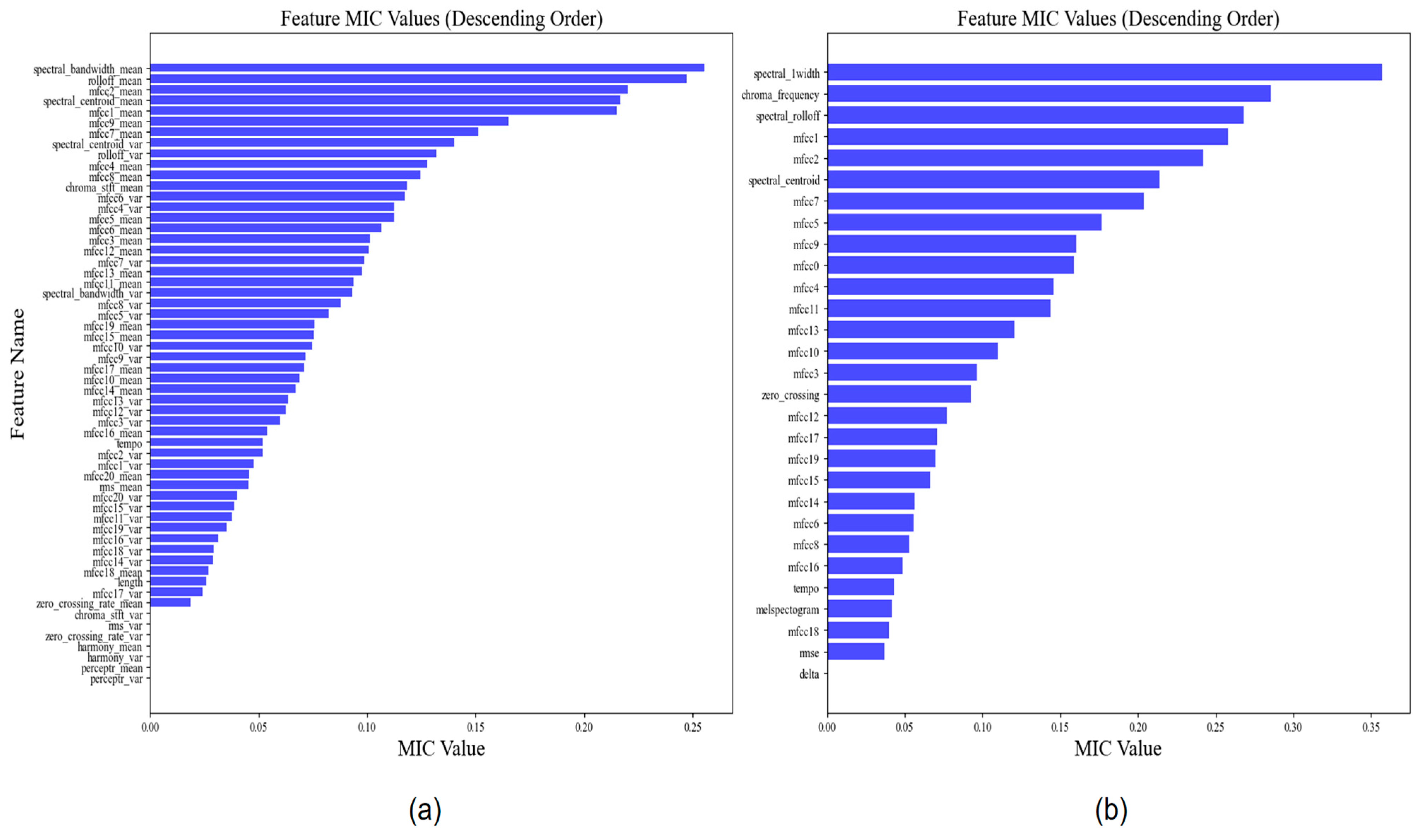
3.4.1. Feature Selection Results

In this section, we describe the feature selection that was conducted with the MIC method. The resultant graphs are shown in Figure 2, and the values of each weight are shown in Table 2.

Figure 2. MIC feature selection.

Table 2. Feature selection.

Data	Features	Weight
GTZAN	spectral_bandwidth_mean	0.2556
	rolloff_mean	0.2473
	mfcc2_mean	0.2201
	spectral_centroid_mean	0.2165
	mfcc1_mean	0.2150
	mfcc9_mean	0.1650
	Mfcc7_mean	0.1512
	spectral_centroid_var	0.1403
	rolloff_var	0.1318
	Mfcc4_mean	0.1275
	Mfcc8_mean	0.1244
	chroma_stft_mean	0.1183
	Mfcc6_var	0.1172
	Mfcc4_var	0.1125
	Mfcc5_mean	0.1123
	Mfcc6_mean	0.1066
	Mfcc3_mean	0.1012
	Mfcc12_mean	0.1006
	Mfcc7_var	0.0984
	Mfcc13_mean	0.0973
	Mfcc11_mean	0.0938
	spectral_bandwidth_var	0.0929
	Mfcc8_var	0.0876
	Mfcc5_var	0.0823
	Mfcc19_mean	0.0755
	Mfcc15_mean	0.0754
	Mfcc10_var	0.0747
	Mfcc9_var	0.0714
	Mfcc17_mean	0.0709
	Mfcc10_mean	0.0688
	Mfcc14_mean	0.0672
	Mfcc13_var	0.0636
	Mfcc12_var	0.0624
	Mfcc3_var	0.0598
	Mfcc16_mean	0.0539
	tempo	0.0519
	Mfcc2_var	0.0518
	Mfcc1_var	0.0475
	Mfcc20_mean	0.0456
	Rms_mean	0.0450
	Mfcc20_var	0.0401
	Mfcc15_var	0.0387
	Mfcc11_var	0.0377
	Mfcc19_var	0.0352
	Mfcc16_var	0.0313
	Mfcc18_var	0.0294
	Mfcc14_var	0.0290
	Mfcc18_mean	0.0270
	length	0.0256
	Mfcc17_var	0.0241
	zero_crossing_rate_mean	0.0184
	chroma_stft_var	0
	Rms_var	0
	zero_crossing_rate_var	0
	harmony_mean	0
	harmony_var	0
	perceptr_mean	0
Bangla	spectral_1width	0.3569
	chroma_frequency	0.2854
	spectral_rolloff	0.2682
	mfcc1	0.2579
	mfcc2	0.2421
	spectral_centroid	0.2141
	Mfcc7	0.2038
	Mfcc5	0.1764
	Mfcc9	0.1603
	Mfcc0	0.1586
	Mfcc4	0.1456
	Mfcc11	0.1437
	Mfcc13	0.1204
	Mfcc10	0.1099
	Mfcc3	0.0965
	zero_crossing	0.0923
	Mfcc12	0.0771
	Mfcc17	0.0710
	Mfcc19	0.0697
	Mfcc15	0.0664
	Mfcc14	0.0564
	Mfcc6	0.0555
	Mfcc8	0.0528
	Mfcc16	0.0483
	tempo	0.0434
	melspectogram	0.0415
	Mfcc18	0.0396
	rmse	0.0370
	delta	0
	perceptr_var	0

Figure 2a shows the MIC feature selection results for the GTZAN dataset, and Figure 2b shows the feature selection results for the Bangla dataset.

3.4.2. Decomposition Results

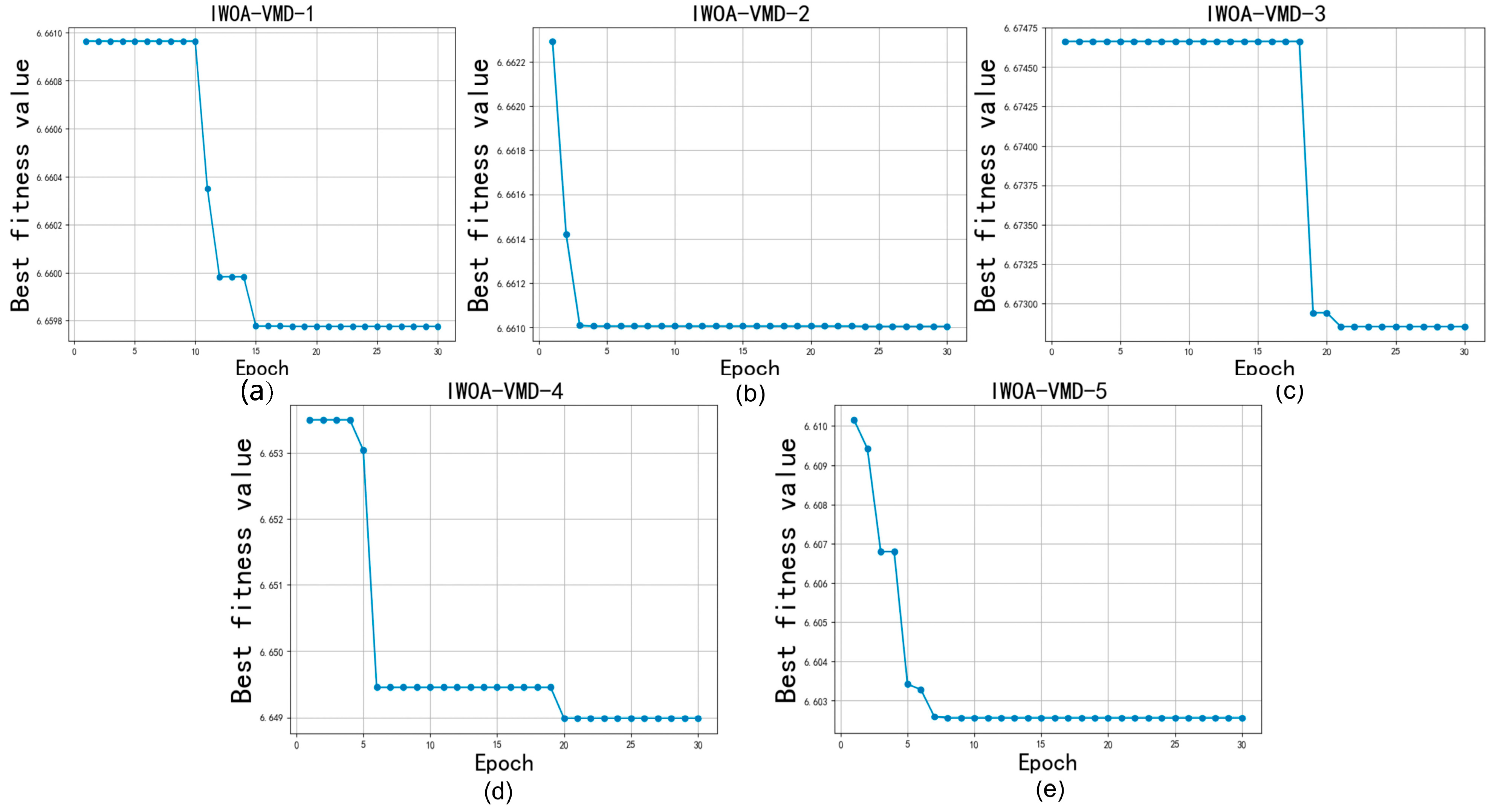
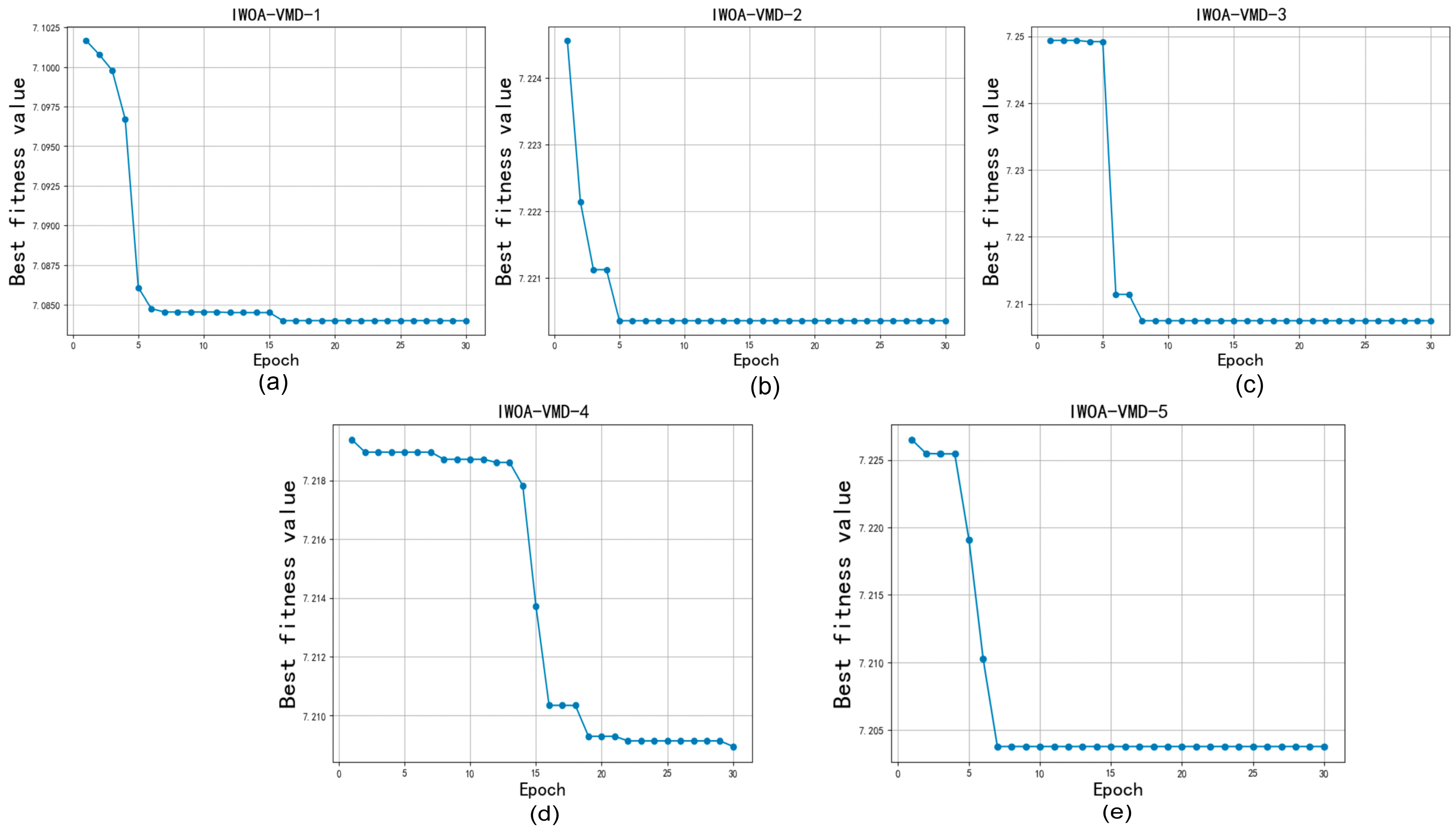
In this subsection, we selected the five features with the highest weight values for decomposition to reduce the accuracy impact of the high complexity and non-linearity of the data. Since the number of decompositions and the penalty factor alpha have a more obvious effect on the decomposition, the parameters of VMD needed to be optimized. We first optimized the K value and alpha of the VMD through IWOA to ensure the best decomposition effect and then set the population of IWOA to 10 and the number of iterations to 30. The optimization process is shown in Figure 3 and Figure 4, and the decomposition process of the VMD is shown in Figure 5 and Figure 6.

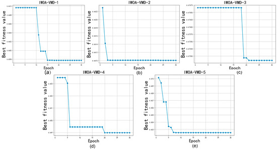
Figure 3. IWOA optimize VMD for GTZAN.

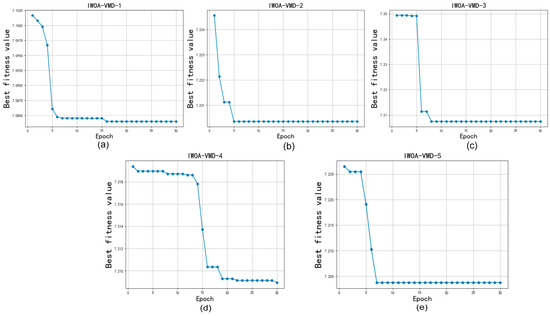
Figure 4. IWOA optimize VMD for Bangla.

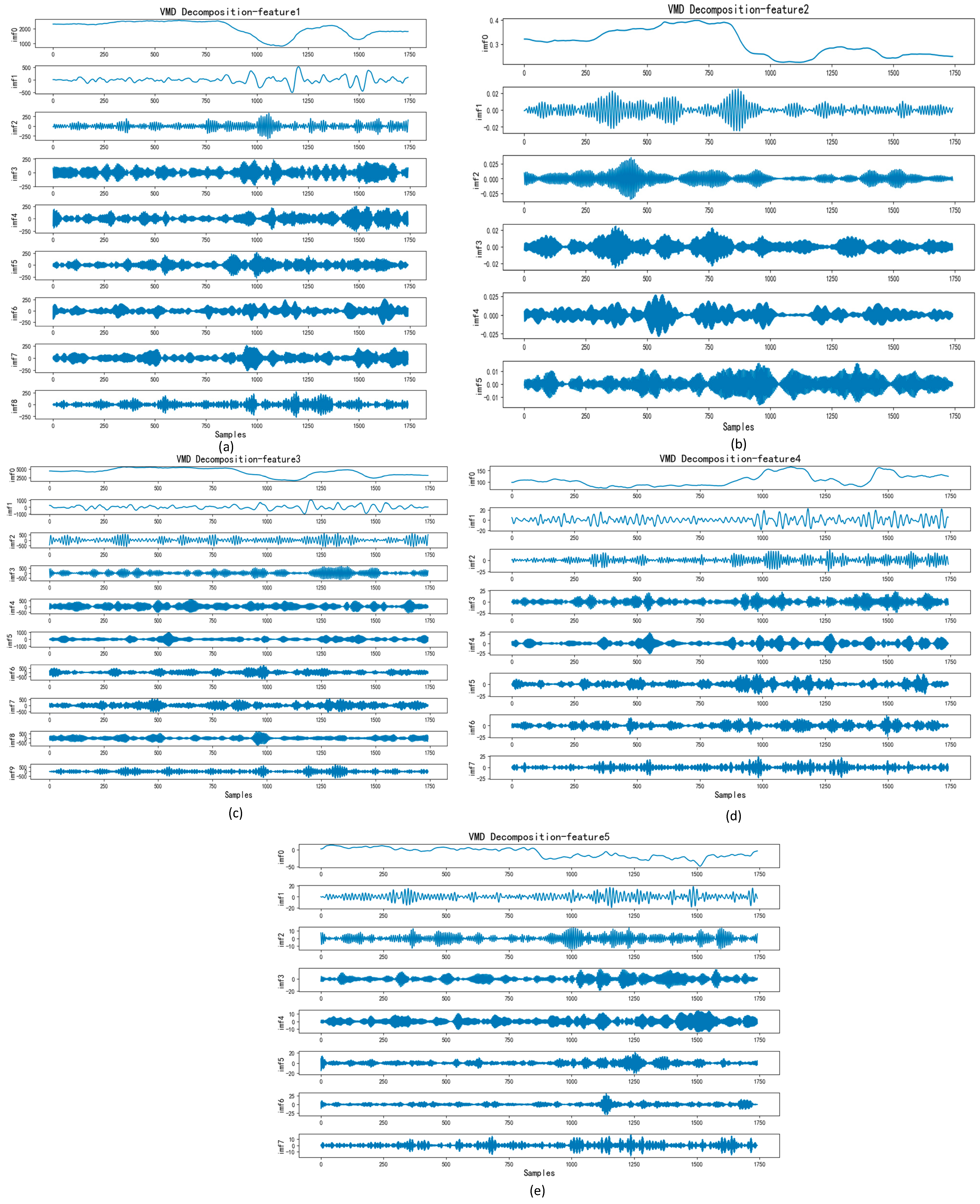
Figure 5. VMD decomposition for GTZAN.

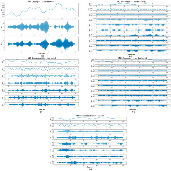
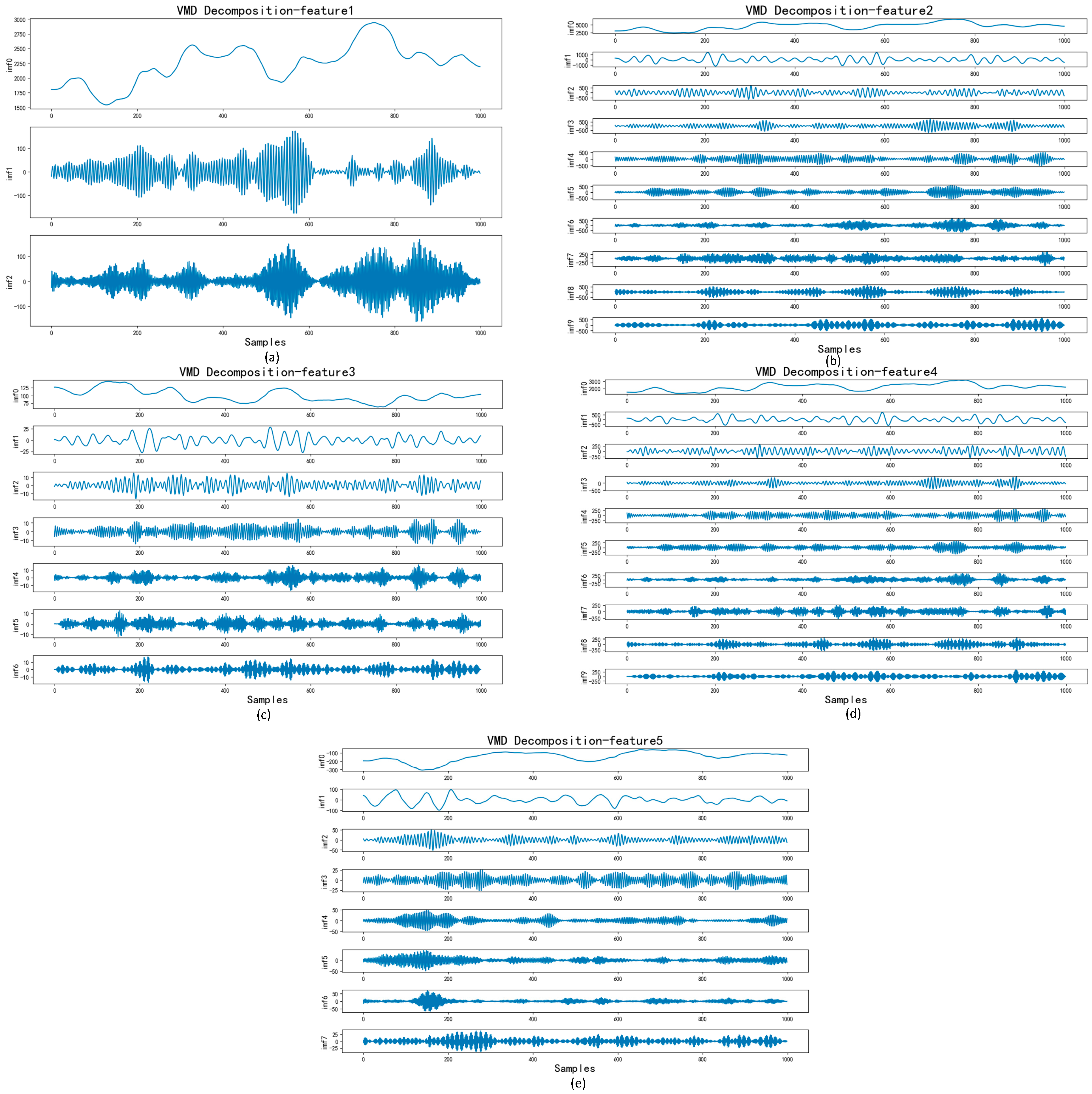
Figure 6. VMD decomposition for Bangla.

Figure 5 illustrates the VMD decomposition process, showcasing the decomposition of features with the highest weight from GTZAN selected by MIC. From Figure 5a–e, the IMF components depict a progressive reduction in data volatility, indicating a continuous decrease in signal complexity throughout the process.

Figure 6 displays the VMD decomposition process of Bangla’s corresponding features. As depicted in Figure 6a–e, the complexity of the data continues to diminish, indicating a clear reduction in complexity throughout the decomposition process.

3.4.3. Analysis of Classification Results

In order to verify the performance and generalization of the VMD-IWOA-XGBOOST model, in this section, we set up a comparison test using different classifiers for comparison. The classification results of the various models are presented in the form of confusion matrices. As illustrated in Figure 7 and Figure 8, the summation of matrix elements yields the aggregate count of songs within the test set. In the confusion matrix representation, the x-axis denotes the sequential indexing of predicted music genres, while the y-axis signifies the sequential indexing of actual music genres. The diagonal elements represent the count of accurately classified genres.

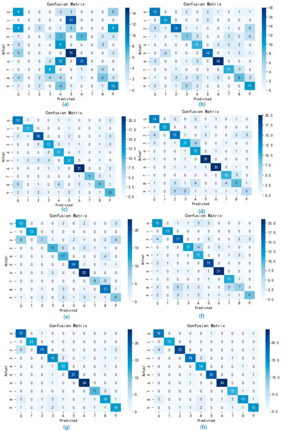
Figure 7. Confusion matrix of the GTZAN experiments.

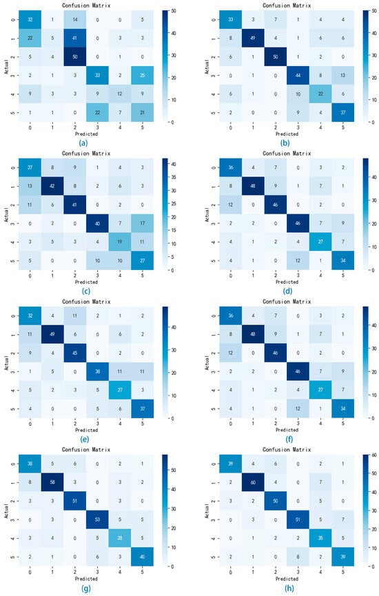
Figure 8. Confusion matrix of the Bangla experiments.

Figure 7a shows the confusion matrix using the AdaBoost classifier experiment weights on the GTZAN test set, where the accuracy value is 0.335, the macro-precision is 0.276, the macro-recall is 0.319, and the macro-F1-score value is 0.271. Figure 8a shows the confusion matrix using the AdaBoost classifier experiment weights on the Bangla test set, where the accuracy value is 0.438, the macro-precision is 0.427, the macro-recall is 0.447, and the macro-F1-score value is 0.405. The classification outcomes derived from the AdaBoost classifier exhibit a notable deficiency in performance, failing to produce satisfactory results.

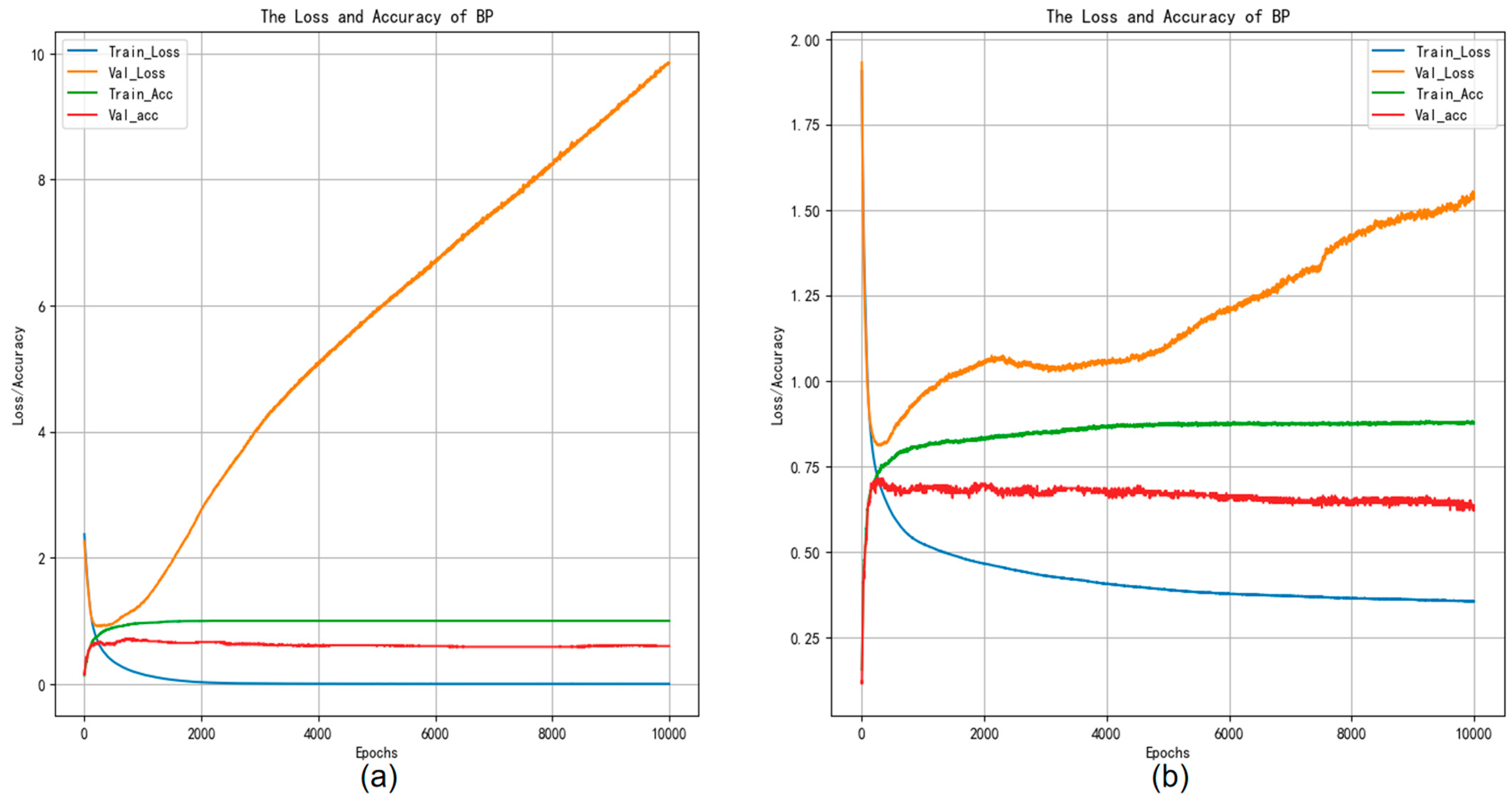
Figure 7b shows the confusion matrix using the BP neural network classifier experiment weights on the GTZAN test set. The classification outcomes are summarized as follows: the accuracy value is 0.625, the macro-precision is 0.648, the macro-recall is 0.639, and the macro-F1-score value is 0.639. Figure 8b shows the confusion matrix using the BP neural network classifier experiment weights on the Bangla test set, and the accuracy value is 0.647, the macro-precision is 0.637, the macro-recall is 0.638, and the macro-F1-score value is 0.636. From this result, we can conclude that the performance of our proposed model surpasses that of the AdaBoost model. Moreover, Figure 9 depicts the accuracy versus loss function curve of the BP neural network.

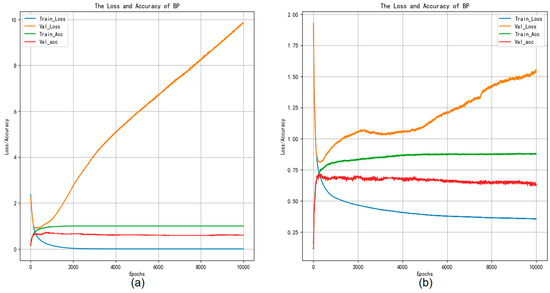
Figure 9. Accuracy and loss curves of the BP experiments training.

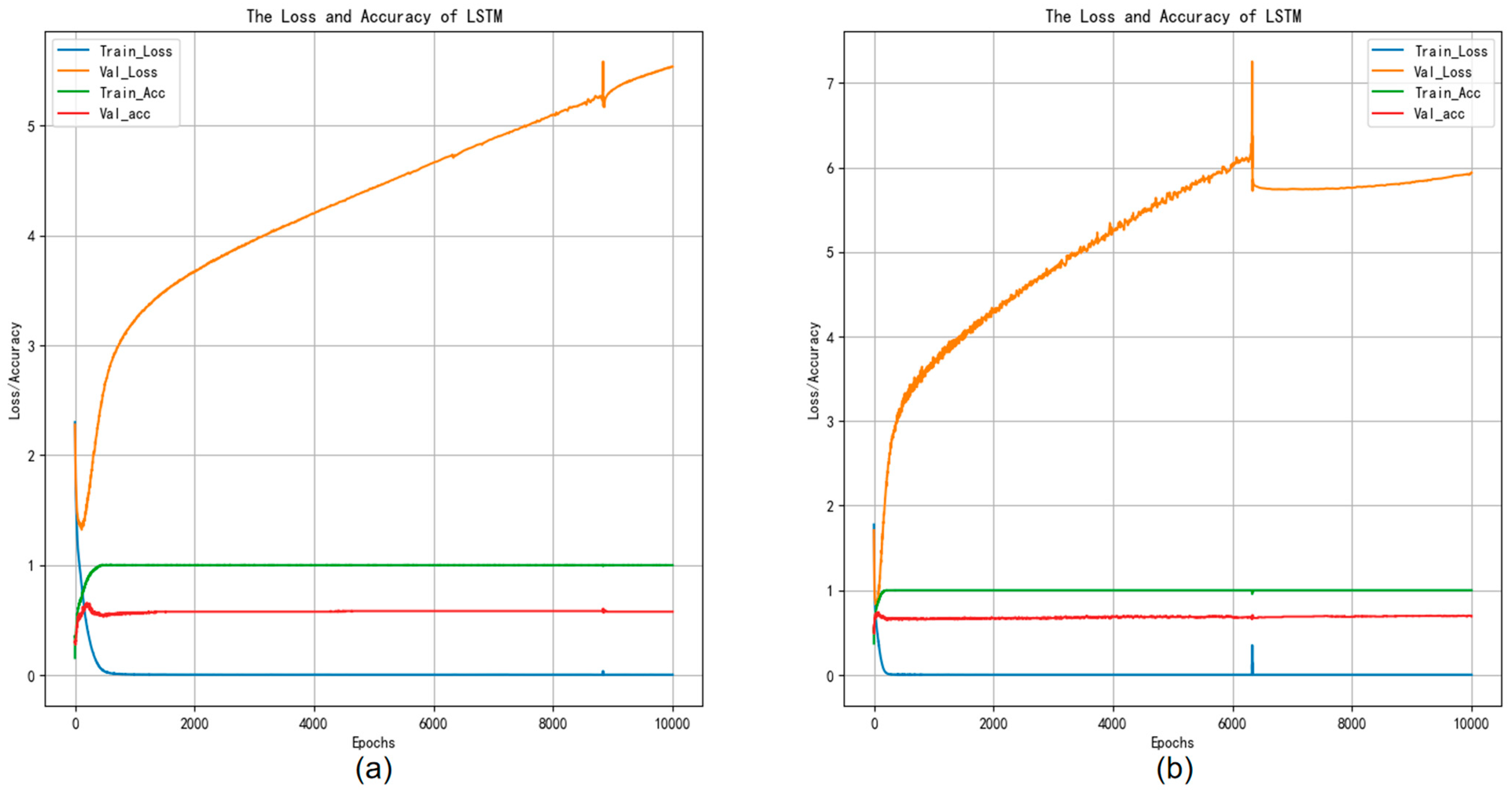
Figure 7c shows the confusion matrix using the LSTM neural network classifier experiment weights on the GTZAN test set. The results can be summarized as follows: the accuracy value is 0.645, the macro-precision is 0.661, the macro-recall is 0.653, and the macro-F1-score value is 0.647. Figure 8c shows the confusion matrix using the LSTM neural network classifier experiment weights on the Bangla test set; the accuracy value is 0.679, the macro-precision is 0.645, the macro-recall is 0.669, and the macro-F1-score value is 0.667. In comparison, based on the experimental results, LSTM demonstrates superior performance over the BP neural network, attributed to its heightened ability in feature extraction across variables, which enhances classification accuracy. Moreover, Figure 10 depicts the accuracy versus loss function curve of the LSTM neural network.

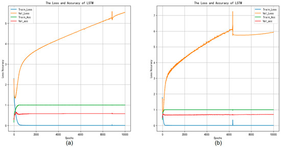
Figure 10. Accuracy and loss curves of the LSTM experiments training.

Figure 7d shows the confusion matrix using the GBDT classifier experiment weights on the GTZAN test set. The classification outcomes can be summarized as follows: the accuracy value is 0.64, the macro-precision value is 0.649, the macro-recall is 0.661, and the macro-F1-score value is 0.642. Figure 8d shows the confusion matrix using the GBDT classifier experiment weights on the Bangla test set. The classification outcomes are summarized as follows: the accuracy value is 0.679, the macro-precision is 0.676, the macro-recall is 0.676, and the macro-F1 score value is 0.673. In contrast, according to the experimental findings, GBDT exhibits similar classification performance to LSTM while offering quicker training speeds.

Figure 7e shows the confusion matrix using the RF classifier experiment weights on the GTZAN test set. The classification results are summarized as follows: the accuracy value of the RF classifier is 0.655, the macro-precision value is 0.687, the macro-recall is 0.673, and the macro-F1-score is 0.659. Figure 8e shows the confusion matrix using the GBDT classifier experiment weights on the Bangla test set, and the accuracy value is 0.653, the macro-precision is 0.653, the macro-recall is 0.659, and the macro-F1-score value is 0.659. Based on these findings, RF not only outperforms LSTM and GBDT in classification but also provides quicker training speeds, making it a good choice for classification modeling.

Figure 7f shows the confusion matrix using the XGBOOST classifier experiment weights on the GTZAN test set. The classification outcomes can be summarized as follows: the accuracy value of the XGBOOST classifier is 0.665, the macro-precision is 0.678, the macro-recall is 0.686, and the macro-F1-score is 0.665. Figure 8f shows the confusion matrix using the XGBOOST classifier experiment weights on the Bangla test set, where the accuracy value is 0.689, the macro-precision is 0.674, the macro-recall is 0.675, and the macro-F1 score value is 0.672. These results exceed those of all previously mentioned models, establishing it as our benchmark model for optimization.

We enhanced XGBOOST to achieve higher classification accuracy, leveraging its exceptional performance among numerous classification models as a guiding factor. Using the WOA algorithm, we optimized the parameters of XGBOOST, including the number of estimators, maximum depth, learning rate, and gamma, aiming to enhance its classification performance. The optimized results surpassed those of XGBOOST without WOA optimization. Figure 7g shows the confusion matrix using the WOA-XGBOOST classifier experiment weights on the GTZAN test set, where the accuracy was 0.765, the macro-precision was 0.767, the macro-recall was 0.776, and the macro-F1-score was 0.767. Figure 8g shows the confusion matrix using the XGBOOST classifier experiment weights on the Bangla test set. The classification results are summarized as follows: the accuracy is 0.767, the macro-precision is 0.759, the macro-recall is 0.759, and the macro-F1-score value is 0.759. The results above demonstrate that the optimized XGBOOST exhibits enhanced proficiency in genre classification.

Recognizing the intricate and volatile nature of numerical music features, we employed decomposition techniques to alleviate the complexity of features, thereby improving classification accuracy. Initially, we identified the five most heavily weighted features using MIC. Following that, we utilized VMD to optimize the decomposition parameters, such as the decomposition number “K” and penalty factor “alpha”, employing the IWOA to attain optimal decomposition performance. After decomposition, the dataset was split into training and test sets with a 0.8:0.2 ratio. Subsequently, XGBOOST was optimized using the IWOA for final classification. Figure 7h shows the confusion matrix using the VMD-IWOA-XGBOOST classifier experiment weights on the GTZAN test set. The following is a summary of the classification outcomes: the accuracy value of VMD-IWOA-XGBOOST is 0.855, the macro-precision is 0.854, the macro-recall is 0.866, and the macro-F1-score value is 0.855. Figure 8h shows the confusion matrix using the VMD-IWOA-XGBOOST classifier experiment weights on the Bangla test set. In summary, the accuracy is 0.785, the macro-precision is 0.782, the macro-recall is 0.782, and the macro-F1-score value is 0.780. These results illustrate the significantly enhanced performance of the decomposed and reclassified model compared to other comparative models, highlighting its superior generalization ability, and providing a novel reference framework for tackling music classification challenges.

From Figure 9a,b, it can be observed that when the training loss decreases but remains unchanged, while the test loss continues to rise, overfitting may be occurring. This indicates that the model performs admirably on the training set, yet demonstrates subpar performance on the test data, signifying a lack of generalizability to novel datasets.

Figure 10a indicates that after a decrease in training loss, the testing loss continues to rise, indicating a certain degree of overfitting, resulting in poor classification and generalization performance of the model on the testing dataset. In Figure 10b, the test loss initially rises, then declines and tends to stabilize, while the training loss remains unchanged. This indicates a bottleneck in the learning process, with suboptimal performance on the test set, resulting in weaker performance in music genre classification.

The comparative results are shown in Table 3. It can be shown that the proposed model is superior to the other benchmark models in terms of four evaluation metrics on two datasets.

Table 3. Comparison between the results using the proposed method and the results using other methods.

Data	Model	Accuracy	MCC	Macro-Precision	Macro-Recall	Macro-F1-Score
GTZAN	AdaBoost	0.335	0.265	0.276	0.319	0.271
	BP	0.625	0.588	0.648	0.639	0.641
	LSTM	0.645	0.660	0.661	0.653	0.647
	GBDT	0.640	0.601	0.649	0.661	0.642
	RF	0.655	0.620	0.687	0.673	0.659
	XGBOOST	0.665	0.630	0.678	0.686	0.665
	WOA-XGBOOST	0.785	0.760	0.787	0.796	0.790
	VMD-IWOA-XGBOOST	0.855	0.844	0.854	0.866	0.855
Bangla	AdaBoost	0.438	0.339	0.427	0.447	0.405
	BP	0.647	0.583	0.637	0.638	0.636
	LSTM	0.679	0.643	0.645	0.669	0.667
	GBDT	0.679	0.616	0.677	0.676	0.673
	RF	0.653	0.585	0.652	0.652	0.648
	XGBOOST	0.689	0.618	0.674	0.675	0.672
	WOA-XGBOOST	0.767	0.720	0.759	0.759	0.759
	VMD-IWOA-XGBOOST	0.785	0.742	0.782	0.782	0.780

To underscore the superiority of the model proposed in this paper, we conducted a t-test to assess its significance. Utilizing 10-fold cross-validation, we obtained experimental results for each model, followed by t-test analysis to ascertain their significance. Additionally, we measured the running time of each model for comparative reference. Table 4 presents the significant results of the t-test.

Table 4. Model t-test experiment and runtime analysis.

Data	Model	Running Time (s)	p-Values
GTZAN	AdaBoost	6.675	0.000
	BP	329.710	0.027
	LSTM	1422.501	0.010
	GBDT	90.445	0.003
	RF	4.588	0.003
	XGBOOST	4.742	0.011
	WOA-XGBOOST	2382.100	0.350
	VMD-IWOA-XGBOOST	1017.203	/
Bangla	AdaBoost	6.125	0.000
	BP	448.431	0.556
	LSTM	2104.9	0.041
	GBDT	55.12	0.044
	RF	4.322	0.001
	XGBOOST	5.235	0.037
	WOA-XGBOOST	2879	0.376
	VMD-IWOA-XGBOOST	1854.5	/

As depicted in Table 4, the 10-fold cross-validation results of the model proposed in this paper exhibit significant superiority compared to other models, as indicated by the t-test. While the difference may not be pronounced when compared to WOA-XGBOOST, the model’s running speed significantly outpaces that of WOA-XGBOOST.

4. Conclusions

In this paper, we propose a hybrid model which uses signal decomposition, the optimization algorithm, and the machine learning model for music genre classification. Librosa is used to transform the original audio into numerical or symbolic features, MIC is used for feature selection, VMD is employed to reduce the complexity of the original features, IWOA is proposed to optimize the parameters of VMD and XGBOOST, and XGBOOST is used for prediction. In this experimental study, two datasets, GTZAN and Bangla, are used as sample data, and eight different models are selected for comparative experiments. The experimental results for our proposed hybrid model were significantly better than those achieved with other models. The contributions of this paper are summarized as follows:

• A hybrid model with VMD-IWOA-XGBOOST is proposed for music genre classification. MIC is used to screen out five high-correlation features, the signal decomposition technique VMD is chosen to extract the key information of features, IWOA is proposed to improve parameter optimization, and XGBOOST is utilized as the classification model.
• An IWOA is developed by refining the search process, contracting encircling, and altering the spiral position. We propose using an IWOA for parameter optimization. Comparative analysis reveals that the IWOA outperforms the WOA algorithm in terms of four evaluation metrics.

References

- Campobello, G.; Dell’Aquila, D.; Russo, M.; Segreto, A. Neuro-genetic programming for multigenre classification of music content. Appl. Soft Comput. 2020, 94, 106488. [Google Scholar] [CrossRef]
- Oramas, S.; Barbieri, F.; Nieto, O.; Serra, X. Multimodal deep learning for music genre classification. Trans. Int. Soc. Music. Inf. Retr. 2018, 1, 4–21. [Google Scholar] [CrossRef]
- Xie, C.; Song, H.; Zhu, H.; Mi, K.; Li, Z.; Zhang, Y.; Cheng, J.; Zhou, H.; Li, R.; Cai, H. Music genre classification based on res-gated CNN and attention mechanism. Multimed. Tools Appl. 2023, 83, 13527–13542. [Google Scholar] [CrossRef]
- Qiu, L.; Li, S.; Sung, Y. DBTMPE: Deep Bidirectional Transformers-Based Masked Predictive Encoder Approach for Music Genre Classification. Mathematics 2021, 9, 530. [Google Scholar] [CrossRef]
- Nag, S.; Basu, M.; Sanyal, S.; Banerjee, A.; Ghosh, D. On the application of deep learning and multifractal techniques to classify emotions and instruments using Indian Classical Music. Phys. A Stat. Mech. Its Appl. 2022, 597, 127261. [Google Scholar] [CrossRef]
- Costa, Y.M.; Oliveira, L.S.; Silla, C.N. An evaluation of Convolutional Neural Networks for music classification using spectrograms. Appl. Soft Comput. 2017, 52, 28–38. [Google Scholar] [CrossRef]
- Yu, Y.; Luo, S.; Liu, S.; Qiao, H.; Liu, Y.; Feng, L. Deep attention based music genre classification. Neurocomputing 2020, 372, 84–91. [Google Scholar] [CrossRef]
- Cheng, Y.-H.; Kuo, C.-N. Machine Learning for Music Genre Classification Using Visual Mel Spectrum. Mathematics 2022, 10, 4427. [Google Scholar] [CrossRef]
- Almazaydeh, L.; Atiewi, S.; Al Tawil, A.; Elleithy, K. Arabic music genre classification using deep convolutional neural networks (CNNS). Comput. Mater. Contin. 2022, 72, 5443–5458. [Google Scholar] [CrossRef]
- Costa, Y.M.G.; Oliveira, L.S.; Koerich, A.L.; Gouyon, F.; Martins, J.G. Music genre classification using LBP textural features. Signal Process. 2012, 92, 2723–2737. [Google Scholar] [CrossRef]
- Gan, J. Music Feature Classification Based on Recurrent Neural Networks with Channel Attention Mechanism. Mob. Inf. Syst. 2021, 2021, 7629994. [Google Scholar] [CrossRef]
- Kumaraswamy, B. Optimized deep learning for genre classification via improved moth flame algorithm. Multimed. Tools Appl. 2022, 81, 17071–17093. [Google Scholar] [CrossRef]
- Wang, H.; Siti, S.; Chen, Z.; Shan, Q.; Ren, L. An intelligent music genre analysis using feature extraction and classification using deep learning techniques. Comput. Electr. Eng. 2022, 100, 107978. [Google Scholar] [CrossRef]
- Tian, R.; Yin, R.; Gan, F. Music sentiment classification based on an optimized CNN-RF-QPSO model. Data Technol. Appl. 2023, 57, 719–733. [Google Scholar] [CrossRef]
- Li, J.; Han, L.; Wang, Y.; Yuan, B.; Yuan, X.; Yang, Y.; Yan, H. Combined angular margin and cosine margin softmax loss for music classification based on spectrograms. Neural Comput. Appl. 2022, 34, 10337–10353. [Google Scholar] [CrossRef]
- Chudy, M.; Nawrocka-Wysocka, A.; Łukasik, E.; Kuśmierek, E.; Parkoła, T. Incorporating symbolic representations of traditional music into a digital library. In Proceedings of the 10th International Conference on Digital Libraries for Musicology (DLfM ‘23), Milan, Italy, 10 November 2023; Association for Computing Machinery: New York, NY, USA, 2023; pp. 30–34. [Google Scholar] [CrossRef]
- Tzanetakis, G.; Ermolinskyi, A. Cook Pitch histograms in audio and symbolic music information retrieval. J. New Music Res. 2003, 32, 143–152. [Google Scholar] [CrossRef]
- Karydis, I. Symbolic Music Genre Classification Based on Note Pitch and Duration. In Advances in Databases and Information Systems. ADBIS 2006; Lecture Notes in Computer Science; Manolopoulos, Y., Pokorný, J., Sellis, T.K., Eds.; Springer: Berlin/Heidelberg, Germany, 2006; Volume 4152. [Google Scholar] [CrossRef]
- McKay, C.; Fujinaga, I. Automatic genre classification using large high-level musical feature sets. In Proceedings of the 5th International Symposium on Music Information Retrieval, Barcelona, Spain, 10–14 October 2004; pp. 1–6. [Google Scholar] [CrossRef]
- Valverde-Rebaza, J.; Soriano, A.; Berton, L.; de Oliveira, M.C.F.; De Andrade Lopes, A. Music Genre Classification Using Traditional and Relational Approaches. In Proceedings of the 2014 Brazilian Conference on Intelligent Systems, Sao Paulo, Brazil, 18–22 October 2014; pp. 259–264. [Google Scholar] [CrossRef]
- Lee, J.; Lee, M.; Jang, D.; Yoon, K. Korean Traditional Music Genre Classification Using Sample and MIDI Phrases. KSII Trans. Internet Inf. Syst. 2018, 12, 1869–1886. [Google Scholar] [CrossRef]
- Qiu, L.; Li, S.; Sung, Y. 3D-DCDAE: Unsupervised Music Latent Representations Learning Method Based on a Deep 3D Convolutional Denoising Autoencoder for Music Genre Classification. Mathematics 2021, 9, 2274. [Google Scholar] [CrossRef]
- Cheng, Y.-H.; Chang, P.-C.; Kuo, C.-N. Convolutional Neural Networks Approach for Music Genre Classification. In Proceedings of the 2020 International Symposium on Computer, Consumer and Control (IS3C), Taichung City, Taiwan, 13–16 November 2020; pp. 399–403. [Google Scholar] [CrossRef]
- Sakinat, O. Folorunso, Sulaimon A. Afolabi, Adeoye B. Owodeyi, Dissecting the genre of Nigerian music with machine learning models. J. King Saud Univ.-Comput. Inf. Sci. 2022, 34, 6266–6279. [Google Scholar] [CrossRef]
- Tzanetakis, G.; Cook, P. Musical genre classification of audio signals. IEEE Trans. Speech Audio Process. 2002, 10, 293–302. [Google Scholar] [CrossRef]
- Al Mamun, M.A.; Kadir, I.; Rabby, A.S.A.; Al Azmi, A. Bangla Music Genre Classification Using Neural Network. In Proceedings of the 2019 8th International Conference System Modeling and Advancement in Research Trends (SMART), Moradabad, India, 22–23 November 2019; pp. 397–403. [Google Scholar] [CrossRef]
- Abou-Abbas, L.; Tadj, C.; Fersaie, H.A. A fully automated approach for baby cry signal segmentation and boundary detection of expiratory and inspiratory episodes. J. Acoust. Soc. Am. 2017, 142, 1318. [Google Scholar] [CrossRef] [PubMed]
- Reshef, D.N.; Reshef, Y.A.; Finucane, H.K.; Grossman, S.R.; McVean, G.; Turnbaugh, P.J.; Lander, E.S.; Mitzenmacher, M.; Sabeti, P.C. Detecting Novel Associations in Large Data Sets. Science 2011, 334, 1518–1524. [Google Scholar] [CrossRef] [PubMed]
- Dragomiretskiy, K.; Zosso, D. Variational Mode Decomposition. IEEE Trans. Signal Process. 2014, 62, 531–544. [Google Scholar] [CrossRef]
- Mirjalili, S.; Lewis, A. The Whale Optimization Algorithm. Adv. Eng. Softw. 2016, 95, 51–67. [Google Scholar] [CrossRef]
- Adilaxmi, M.; Bhargavi, D.; Phaneendra, K. Numerical Solution of Singularly Perturbed Differential-Difference Equations using Multiple Fitting Factors. Commun. Math. Appl. 2019, 10, 681–691. [Google Scholar] [CrossRef]
- Chen, T.; Guestrin, C. XGBoost: A Scalable Tree Boosting System. In Proceedings of the 22nd ACM SIGKDD International Conference on Knowledge Discovery and Data Mining (KDD ‘16), San Francisco, CA, USA, 13–17 August 2016; Association for Computing Machinery: New York, NY, USA, 2016; pp. 785–794. [Google Scholar] [CrossRef]
Disclaimer/Publisher’s Note: The statements, opinions and data contained in all publications are solely those of the individual author(s) and contributor(s) and not of MDPI and/or the editor(s). MDPI and/or the editor(s) disclaim responsibility for any injury to people or property resulting from any ideas, methods, instructions or products referred to in the content. |
© 2024 by the authors. Licensee MDPI, Basel, Switzerland. This article is an open access article distributed under the terms and conditions of the Creative Commons Attribution (CC BY) license (https://creativecommons.org/licenses/by/4.0/).