Abstract
In this study, an inverse conjugate heat transfer problem is examined to estimate temporally and spatially the dependent unknown surface heat flux using thermography techniques with a thermal camera in a three-dimensional domain. Thermography techniques encompass a broad set of methods and procedures used for capturing and analyzing thermal data, while thermal cameras are specific tools used within those techniques to capture thermal images. In the present study, the interface conditions of the plate and air domains are obtained using perfect thermal contact conditions, and therefore we define the problem studied as an inverse conjugate heat transfer problem. Achieving the simultaneous solution of the continuity, Navier–Stokes, and energy equations within the air domain, alongside the heat conduction equation in the plate domain, presents a more intricate challenge compared to conventional inverse heat conduction problems. The validity of our inverse solutions was verified through numerical simulations, considering various inlet air velocities and plate thicknesses. Notably, it was found that due to the singularity of the gradient of the cost function at the final time point, the estimated results near the final time must be discarded, and exact measurements consistently produce accurate boundary heat fluxes under thin-plate conditions, with air velocity exhibiting no significant impact on the estimates. Additionally, an analysis of measurement errors and their influence on the inverse solutions was conducted. The numerical results conclusively demonstrated that the maximum error when estimating heat flux consistently remained below 3% and higher measurement noise resulted in the accuracy of the heat flux estimation decreasing. This underscores the inherent challenges associated with inverse problems and highlights the importance of obtaining accurate measurement data in the problem domain.
Keywords:
inverse conjugate heat transfer problem; conjugate gradient method; spatially and temporally dependent heat flux estimation MSC:
65K10; 65M30; 65M32; 65Q10; 76B99
1. Introduction
Thermography is a technique used to create images of temperature variations on the surfaces of objects by detecting the infrared radiation emitted, utilizing infrared cameras or sensors to measure the radiation. The collected data are then converted into temperature values and displayed as thermal images.
Thermography has applications across various fields. (a) In the medical field, it is used for diagnosing health conditions, detecting anomalies in body temperature, and identifying areas of inflammation or injury; (b) in building inspections, thermography is used to detect energy inefficiencies, moisture intrusion, insulation defects, and structural anomalies in buildings; (c) in electrical inspections, it aids in identifying overheating components, loose connections, and potential faults in electrical systems; (d) in non-destructive testing, it is employed to identify defects, cracks, and anomalies in materials without causing damage to them; and (e) in industrial applications, thermography is utilized for the predictive maintenance of machinery, monitoring manufacturing processes, and detecting hot spots or applied heat fluxes in industrial equipment. Overall, thermography provides valuable insights into temperature distribution and helps diagnose problems or anomalies across various applications. In this study, thermography technology is used to identify unknown applied heat fluxes in inverse problems.
To classify inverse problems, we begin with the presumption of a direct problem rooted in the field of mathematical physics. This implies that when we possess comprehensive knowledge about a physical system, we are equipped with a classical mathematical portrayal of said system, encompassing aspects such as uniqueness, stability, and the existence of solutions for the corresponding mathematical problem. However, when tasked with determining one or more unknown parameters characterizing this system based on additional experimental data, we are faced with an inverse problem.
Recent advancements in mathematical theory have spurred the evolution of efficient methodologies and algorithms to tackle a range of inverse heat transfer problems. Currently, we possess the tools necessary to successfully resolve and practically apply inverse heat transfer problems across various applied research endeavors, as well as in the experimental development of thermal engineering applications.
Inverse heat transfer problems encompass a spectrum of classifications, including inverse heat conduction problems (the most prevalent), inverse heat convection problems, inverse heat radiation problems, and inverse heat conjugation problems. Researchers have comprehensively explored inverse problems related to heat conduction [1,2,3,4,5,6,7,8,9], heat convection [10,11,12,13,14,15,16], and heat radiation [17,18,19], employing diverse algorithms. However, investigations into inverse conjugate heat transfer problems [20,21,22] remain notably scarce within the available literature.
It is worth noting that practical thermal science and engineering applications fall under the purview of direct heat conduction–convection coupled problems. In these scenarios, the velocity, pressure, and temperature distributions within a system can be computed through the implementation of the known initial and boundary conditions. This entails the simultaneous resolution of the continuity, momentum, and energy equations within the fluid domain, along with the energy equation governing the solid domain.
Contrary to direct heat conduction–convection-coupled problems, resolving an inverse heat conduction–convection-coupled problem involves determining either the system’s initial condition, its boundary conditions, or any unknown functions based on the temperatures measured within it. In this scenario, the continuity, momentum, and energy equations must be tackled concurrently. This significantly complicates the computational process, leading to a scarcity of works in the literature addressing this particular challenge.
Among the array of algorithms available for tackling inverse heat transfer problems, gradient-based and self-regularized iterative algorithms stand out as potent optimization tools. This method is particularly renowned for its effectiveness and efficiency when calculating the gradient of a cost function, making it a primary choice for addressing inverse heat transfer problems. Both the steepest descent method (SDM) [23] and the conjugate gradient method (CGM) [23] are gradient-based and self-regularized iterative algorithms. Unlike methods that demand prior knowledge of the functional forms of unknown quantities, these algorithms generate dependable estimates without such prerequisites. As a result, they have emerged as potent tools for function estimation in inverse problems, particularly for addressing three-dimensional challenges.
For example, Zhou et al. [24] utilized the conjugate gradient method (CGM) in an inverse heat conduction problem to estimate the heat flux and temperature distribution on the front surface of a three-dimensional object based on measurements taken on the back surface. Their numerical findings revealed that the CGM was highly effective, accurately estimating the two-dimensional heat flux and temperature distribution on the front surface through inverse estimations. Huang and Wang [25] employed the CGM to tackle a transient three-dimensional heat conduction inverse problem, aiming to estimate the unknown time-dependent boundary heat flux. Their study revealed averaged relative errors of 8.3% and 3.7% for Cases 1 and 2, respectively, with a 2% measurement error.
Huang and Chen [26] utilized the CGM to address a three-dimensional irregular-duct flow problem within the inverse heat convection domain, aiming to estimate the unknown boundary heat flux. Their investigation revealed that the error in the estimated heat flux increased proportionally with the duct thickness. Zhang et al. [27] conducted a study on an inverse heat radiation problem, aiming to simultaneously estimate the radiative properties (namely, the extinction coefficient, scattering albedo, and wall emissivity) of a cylindrical system. They based their analysis on the radiative heat flux measurements obtained from various boundaries and employed the CGM. Their findings demonstrated that the proposed inverse analysis method effectively retrieved the previously unknown radiative physical properties of the cylindrical system.
It should be noted that the above problems are related to inverse heat conduction, convection, or radiation; no inverse heat conjugated problems were investigated. Recently, Huang and He [21] employed the CGM for the first time to determine the unknown space-dependent heat flux in a steady-state 3-D inverse conjugate heat transfer problem, and subsequently [22] conducted experiments to verify the validity of the CGM when estimating the heat flux of a steady-state inverse heat conduction–convection conjugated problem. To our knowledge, the CGM has not been previously applied to address a three-dimensional time-dependent inverse heat conduction–convection conjugated problem.
An advantage of the CGM lies in its ability to handle problems without prior knowledge of the functional form of the unknown functions. This allows for the correction and estimation of a large number of unknowns in each iteration, consistently yielding accurate estimates. In addition, CFD-ACE+ [28] is a commercial computational fluid dynamics solver that solves the conservation equations of mass, momentum, energy, chemical species, and other scalar transport equations using the finite volume method. These equations enable coupled simulations of fluid, thermal, chemical, biological, electrical, and mechanical phenomena. It has been widely employed in numerous studies on inverse problems [21,22] for direct problem computations.
Therefore, the present study demonstrates the first use of the CGM for optimization, utilizing CFD-ACE+ as a computational tool, to address a 3-D transient inverse conjugate heat transfer problem that predicts boundary heat flux, which varies both spatially and temporally.
2. The Direct Problem
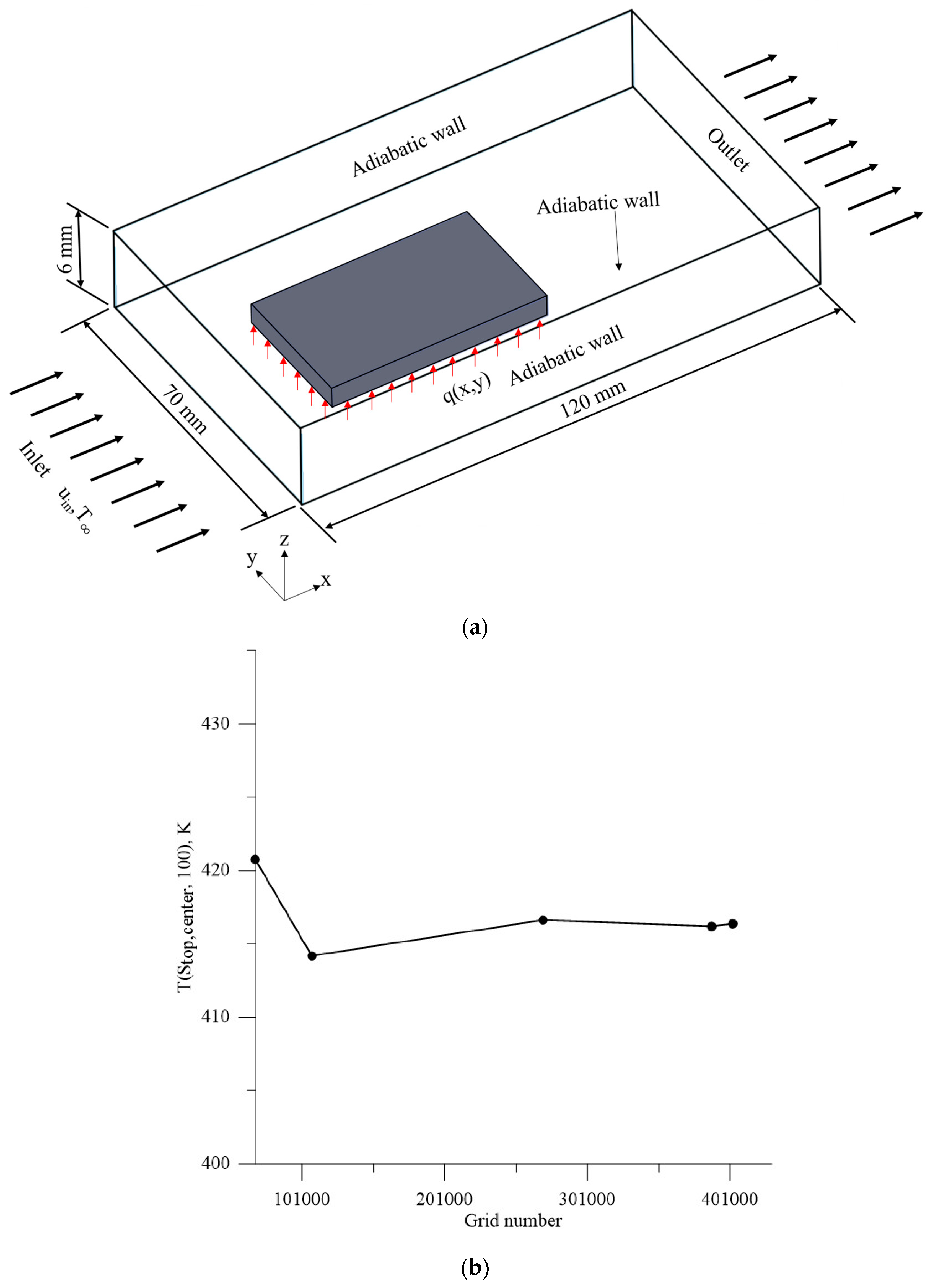
The CGM was employed in conjunction with thermography technology to predict the bottom surface heat flux, which is a function of space and time in a three-dimensional inverse conjugate heat transfer problem, of a rectangular plate. The computational domain, denoted as Ω, consists of two sub-domains: a plate sub-domain, Ωp, and an air sub-domain, Ωa. The flat plate is positioned within a rectangular duct, where its lower surface Sbottom experiences an unknown heat flux, q(Sbottom,t), while incompressible ambient air with the inlet velocity and ambient temperature Uin and , respectively, flows into Ω, contributing to the cooling of the rectangular plate. The initial temperature conditions for both Ωp and Ωa are set as equal to the ambient temperature .
The boundary interface surfaces between Ωp and Ωa adhere to the perfect thermal contact condition, ensuring that the temperature and heat flux of the plate match those of the air on the interface surfaces. Figure 1 illustrates the geometry and computational domain considered in the present work.
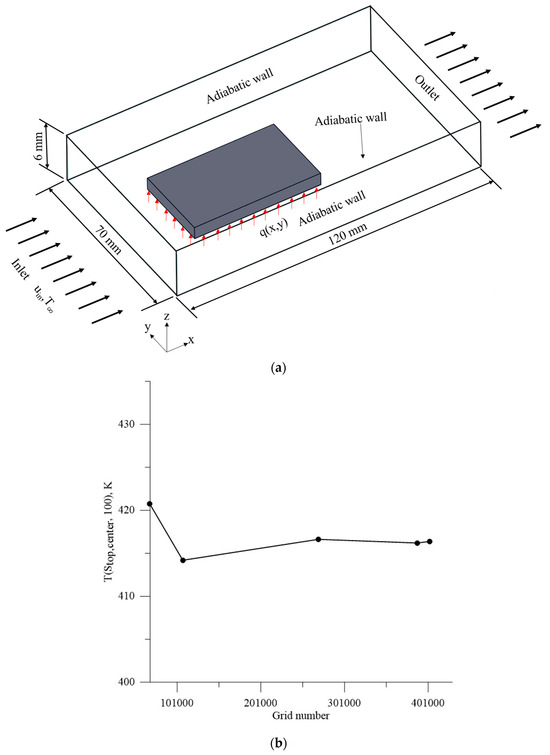
Figure 1.
(a) The computational domain and model geometry used in this study and (b) the plots of the grid independence test.
The mathematical models for the present direct problem are illustrated below.
- (I)
- Plate domain (Ωp)
The initial condition of the plate is equal to , and an unknown heat flux q(Sbottom) is applied to the bottom surface Sbottom, i.e.,
- (II)
- Air domain (Ωa)
The mathematical models for the continuity, Navier–Stokes, and energy equations for the air domain are as follows:
Here, ka, ρa, cpa, Ta, and U symbolize the air thermal conductivity, density, heat capacity, temperature, and velocity vector, respectively. The inlet and initial conditions of air are given below:
The viscous dissipation function, denoted as Φ, is specified as:
- (III)
- Plate–air interface ()
The interface conditions of Ωp and Ωa are as follows:
The software package CFD-ACE+ is utilized to compute the solutions for the above direct problem in Ω.
3. The Inverse Problem
In the context of the 3-D inverse heat conduction–convection-coupled problem under consideration, the boundary heat flux q(Sbottom,t) is regarded as unknown, varying in both space and time. All other terms in Equations (1)–(8) are known. The temperature measurements captured on Stop using a thermal camera are deemed available.
Consider the temperature reading for Stop, denoted as Yp(Stop,t) ≡ Yk,m, where k ranges from 1 to K and m ranges from 1 to M. Here, k and m represent the measured temperatures for different times and positions on Stop. It is important to note that Yp(Stop,t) should contain errors for measurements. The addressed inverse problem is resolved by utilizing Yp(Stop,t) to estimate the heat flux q(Sbottom,t).
The objective is to minimize the following cost function in order to estimate q(Sbottom,t):
where Tk,m represent the computed values at (xm,ym,tk) and indicates the Dirac delta function.
4. CGM for Minimization
The iterative-based CGM [23] given below is considered to estimate the unknown heat flux q(Sbottom,t) by minimizing the cost function J[q(Sbottom,t)]:
Here, is the search step size and Pn(Sbottom,t) is the direction of descent, which can be obtained using the following equation:
where is the gradient of the cost function and the conjugate coefficient γn can be computed from
The values of and must be known prior to computing the iterative Equation (10). The values of and can be obtained by utilizing the solutions of the following sensitivity and adjoint problems.
4.1. The Sensitivity Functions
The sensitivity functions are formulated by introducing a perturbation to the unknown heat flux in the original direct problem described by Equations (1)–(8) through the following steps. In the direct problem, q, Tp, and Ta are replaced by q + Δq, Tp + ΔTp, and Ta + ΔTa, resulting in the perturbed problem, where Δ represents the perturbed value. Subsequently, the direct problem is subtracted from the perturbed problem and the higher-order terms are neglected; the sensitivity problem can then be derived.
For the linear problem considered here, the perturbation of the heat flux Δq does not influence the values of U and P derived from Equations (3) and (4); therefore, Equations (3) and (4) only need to be solved once for all subsequent iterations.
- (I)
- Plate domain (Ωp)
Here, the initial and boundary conditions of the sensitivity problem are as follows:
Tp(Ωp,0) = 0 at t = 0
- (II)
- Air domain (Ωa)
The corresponding energy equation is shown below.
The inlet and initial conditions for the sensitivity function in Ωa can be obtained as follows:
Uin = uin and ΔTa,in = 0, t > 0
ΔTa(Ωa,0) = 0
- (III)
- Plate–air interface ()
The interface conditions are defined as follows:
The sensitivity problem outlined above is tackled using CFD-ACE+.
To ascertain the value of , a modified cost function is given below. In Equation (9), is initially replaced by and subsequently linearized using a Taylor expansion, resulting in the expression given below:
The solution of Equations (13)–(17) can be solved by using [23]. Minimizing Equation (18) with respect to yields the following expression for the determination of :
4.2. The Adjoint Functions
The adjoint functions are acquired through the following process. Equations (1) and (5) are multiplied by λp and λa, respectively, and the resultant expressions are integrated over the corresponding time domain t and spatial domains Ωp and Ωa. Subsequently, the outcomes are added to the right-hand side of Equation (9) to formulate the following functional J[q(Sbottom,t)]:
The variation ΔJ can be determined by introducing the perturbations Δq to q, ΔTp to Tp, and ΔTa to Ta in Equation (20). By subtracting the original Equation (20) from the perturbed expression and neglecting second and higher order terms, the following equation is obtained:
Green’s second identity is applied to simplify the last two integration terms in Equation (21); Equations (14b) and (17) are utilized; and as ΔJ approaches zero, the integrands involving ΔTp and ΔTa vanish. This process results in the following adjoint problem for solving the adjoint functions λp and λa.
- (I)
- Plate domain (Ωp)
λp(Ωp,tf) = 0
- (II)
- Air domain (Ωa)
The inlet and final conditions in Ωa are as follows:
Uin = uin and λa,in = 0, t > 0
λa(Ωa,tf)= 0
- (III)
- Plate–air interface ()
The interface conditions for the surface are as follows:
The interface condition for Stop is as follows:
Equation (27) suggests that there are additional applied heat sources on the interface surface Stop for the adjoint problem.
In addition, it is noted that the form of energy equations for the adjoint problems in Ωp and Ωa, i.e., Equations (22) and (24), are different from the direct and sensitivity problems; instead of the traditional initial value problem, they become the final time value problem, and the final condition at time t = tf is specified, i.e., as in Equations (23a) and (25b). However, these problems can be transformed into an initial value problem by the transformation of the time variables to τ = tf − t. Thereafter, the form of the energy equations becomes identical to those of the direct and sensitivity problems, and then the solutions to the adjoint functions outlined above can be obtained using CFD-ACE+.
Eventually, the following expression for the perturbation of cost function remains.
In addition, the perturbation of the cost function can be obtained as follows [23]:
A comparison of Equations (28) and (29) results in the expression of the gradient of the cost function :
From Equations (23a) and (25b), it is evident that the final time conditions for the adjoint functions λp(Ωp,tf) and λa(Ωa,tf) are both equal to zero. This indicates that the gradient of the cost function is consistently zero at t = tf. Consequently, no corrections can be made at t = tf, and the estimated heat flux will perpetually equate to the initial guess value.
In addition, estimations in the proximity of t = tf will suffer distortion due to singularity at this point. To mitigate the influence of this final time effect on estimation accuracy, extending the computational time domain is recommended. For instance, when estimating heat flux between 1 and 95 s, extending the time domain to tf = 100 s is recommended.
4.3. Discrepancy Principle
The accuracy of any inverse problem relies entirely on the quality of the measurement data. Utilizing precise measuring instruments is imperative, and fine-tuning these instruments is also essential for acquiring the best possible measurement data.
For errorless measured data, the stopping criterion can be defined as
Here, ε is a small, specified number. However, in practical scenarios where measurement temperatures include errors, the cost function is not anticipated to converge to ε due to the ill-posed nature of the inverse problem.
The discrepancy principle [21,22] is then employed to determine the value of ε. The difference between the estimated and measured temperatures is assumed to be σ:
Here, σ is the standard deviation of the measurements. Equation (32) is substituted into Equation (9) to obtain the stopping criterion ε:
ε = KMσ2
5. Results and Discussion
The objective of this work is to employ the CGM for estimating the temporally and spatially varying boundary heat flux q(Sbottom,t) in a 3-D inverse conjugate heat transfer problem. This investigation operates under the assumption of lacking any prior knowledge regarding the functional form of the unknown parameters. Thus, the task at hand is a function estimation within the realm of inverse problems.
In this study, we examined a rectangular plate with the dimensions of Lx = 50 mm, Ly = 30 mm, and Lz = 1 mm. Additionally, a duct with the dimensions of was considered. The heating duration was fixed at 100 s for this investigation.
To discretize the problem, the plate was divided into a grid with 80, 60, and 4 elements along the x, y, and z directions, respectively, and 100 divisions along the time axis. The Sbottom of the plate experienced the heat flux q(Sbottom,t), while the remaining surfaces were subject to a conjugate heat transfer boundary condition. Moreover, an ideal thermal contact condition was enforced across all interface surfaces between the plate and air.
The CFD-ACE+ software was employed to compute the center-point temperature at t = 100 s, T(Stop,center,100), for Q = 10 W, uin = 5 m/s, and = 300 K. Five different grid sizes, 68,640, 108,000, 270,000, 388,800, and 403,200, were tested, yielding temperatures of 420.701 K, 414.165 K, 416.597 K, 416.169 K, and 416.351 K, respectively. When comparing the results between the grid sizes of 270,000 and 388,800, the relative error in T(Stop,center,100) was merely 0.103%. Consequently, 270,000 grid numbers were chosen for the subsequent computations. The plots of the grid independence test are illustrated in Figure 1b.
Two examples with different forms of heat fluxes were examined to validate the efficacy of the CGM when forecasting the unknown q(Sbottom,t) on the bottom surface. This prediction was based on the simulated temperatures obtained on Stop.
Measurement data with random errors were simulated in this work. These errors were generated using normally distributed, uncorrelated errors with a zero mean and a constant standard deviation. This process resulted in the creation of the following set of simulated measurement data, denoted as Y:
Y = Yexact + ω σ
In the context of this representation, Yexact signifies the temperatures for Stop, corresponding to the exact heat flux q(Sbottom,t). The symbol σ denotes the standard deviation in the measured temperatures, while ω is a random number generated within the range of −2.576 to 2.576 by the IMSL subroutine DRNNOR [29], intended to establish a 99% confidence bound.
An advantageous aspect of employing the CGM for computing the inverse problem lies in the flexibility it offers in selecting initial guesses for the unknown quantities. Thus, for all investigated cases in this study, the initial guess q(Sbottom,t)0 = 0.1 was considered arbitrary.
(A) Example 1
The unknown q(x,y,t) on Stobottom is assumed to be a step function, as outlined below:
The step function is independent of positions x and y on the surface Sbottom, with its values varying solely with time.
The plate is discretized into a grid with 80, 60, and 100 divisions along the x, y, and t directions. Consequently, a total of 480,000 unknown discretized values of q(Sbottom,t) need to be estimated over (Sbottom,t), while 480,000 extractions of the measured temperatures obtained by an infrared camera are assumed to be available for the Stop surface. Below, the numerical experiments conducted to estimate the unknown q(Sbottom,t) using the CGM are outlined.
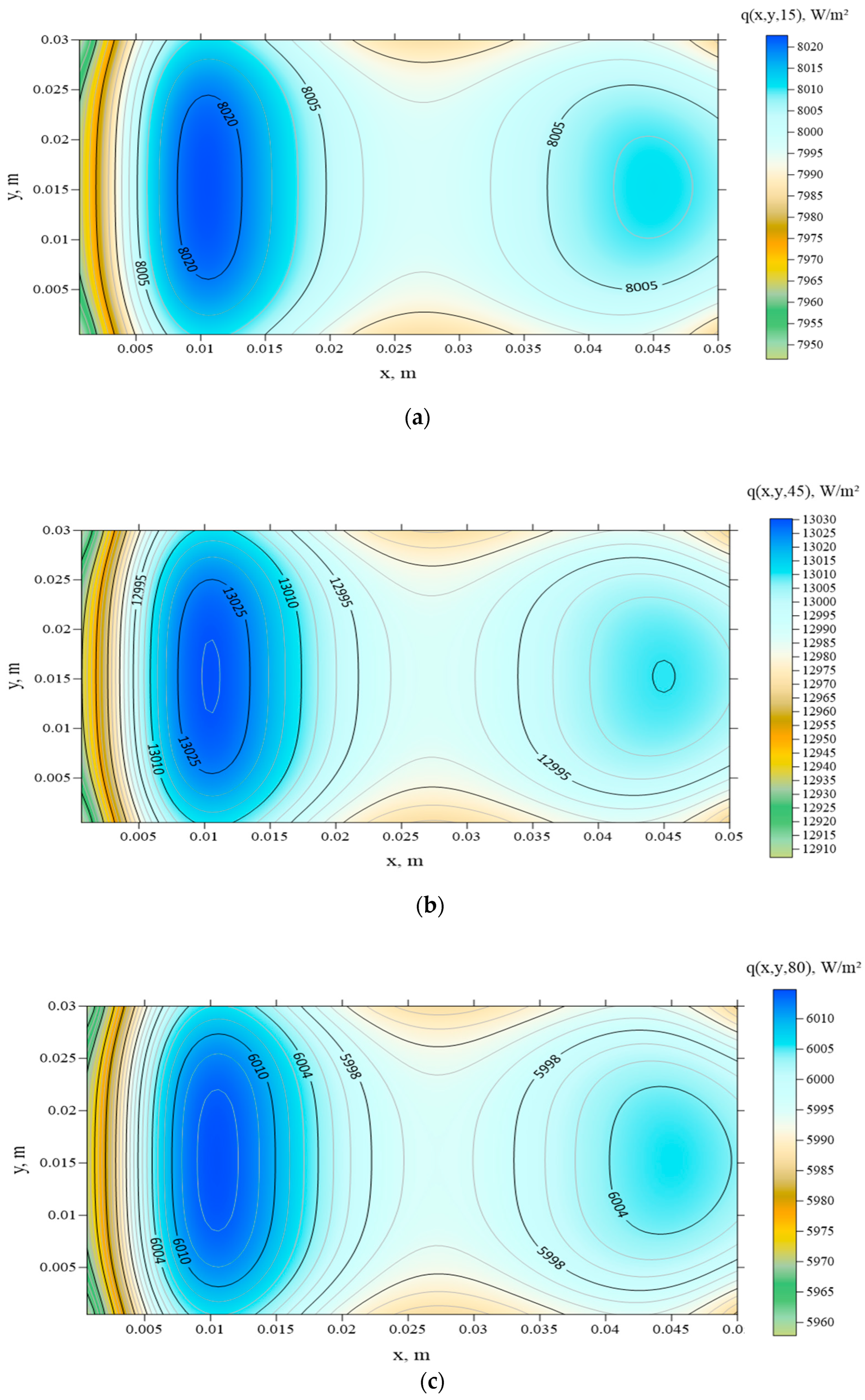
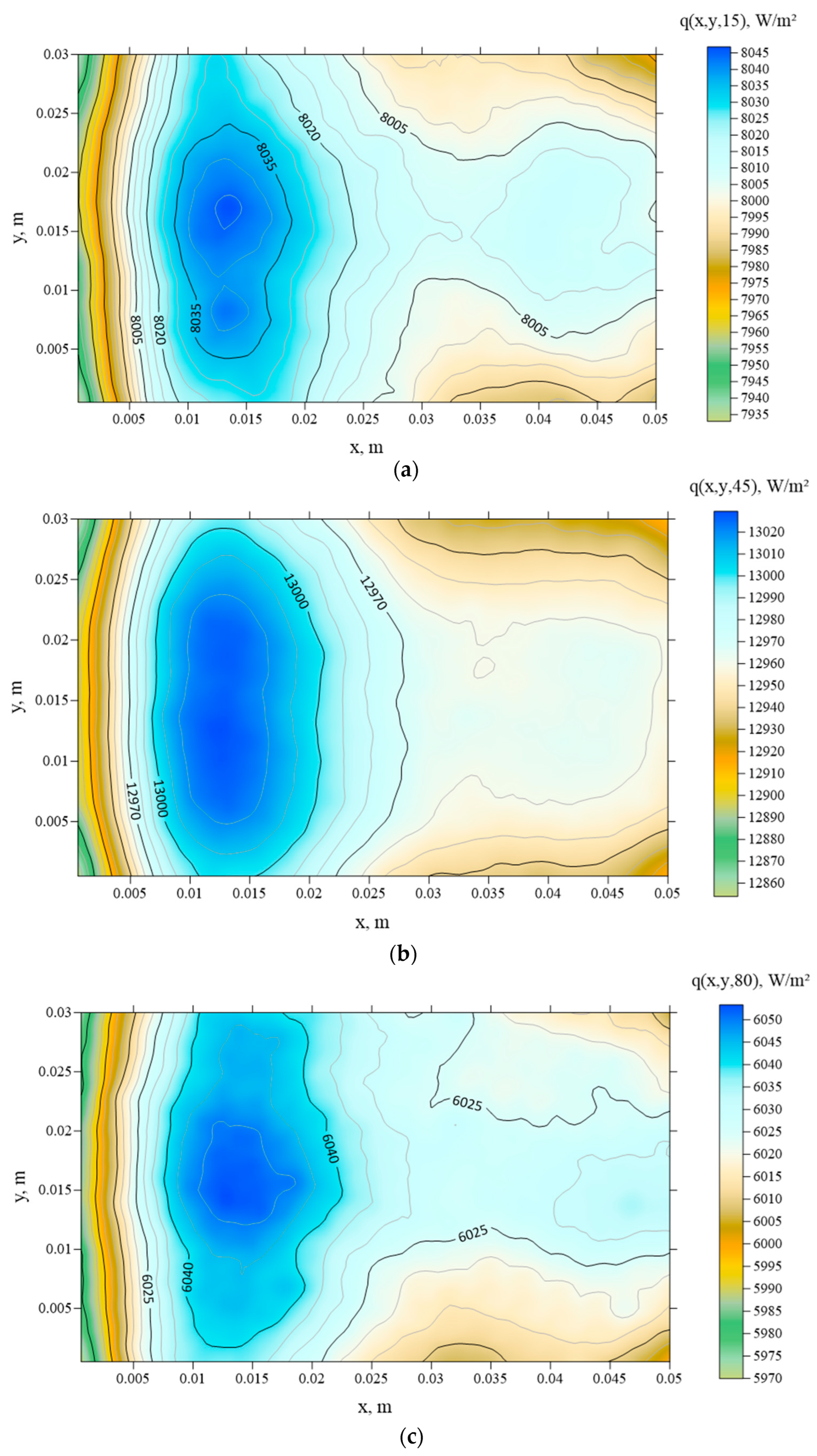
Initially, the inverse problem is conducted assuming that σ = 0.0, uin = 5 m/s, Tp(Ωp,0) = Ta(Ωa,0) = = 300 K, and Lz = 1 mm, corresponding to a thin-plate condition. The cost function decreases to 13 after 100 iterations. Contour plots depicting the estimated heat fluxes at t = 15, 45, and 80 s are presented in Figure 2a–c, respectively. These figures reveal that with exact measurements, the estimated values closely match the exact heat flux described by Equation (35).

Figure 2.
Two-dimensional plots of the estimated heat fluxes over Sbottom at t = (a) 15, (b) 45, and (c) 80 s when σ = 0, Lz = 1 mm, and uin = 5 m/s in Example 1.
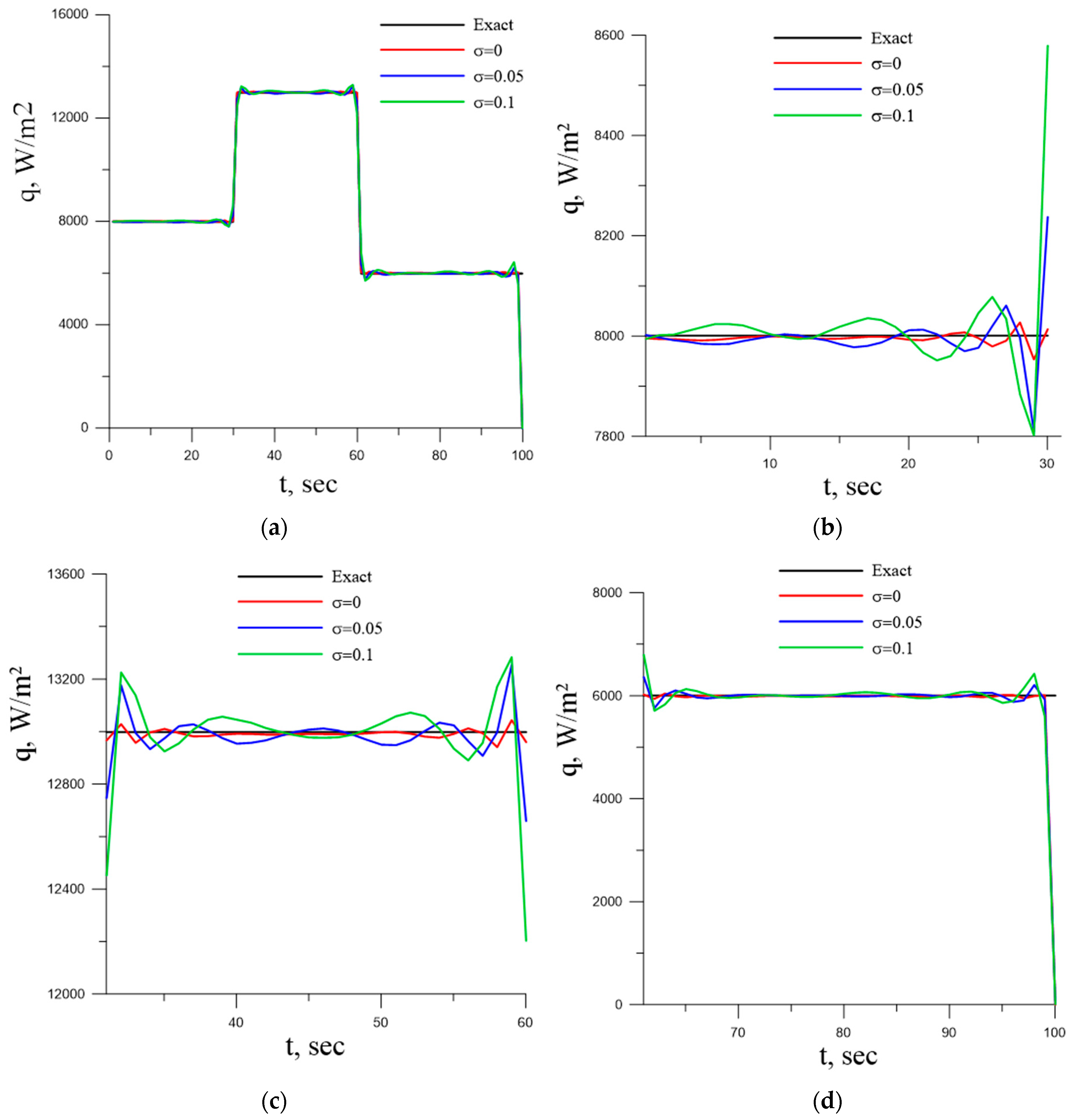
To provide a clearer presentation of the inverse solutions, the exact and estimated q(Sbottom,t) values when σ = 0 at (0.025 m, 0.015 m, 0.0 m) for (a) 0 < t < 100, (b) 0 < t < 30, (c) 30 < t < 60, and (d) 60 < t < 100 s are depicted in Figure 3a–d, respectively. It is notable that the estimated heat flux near the discontinuity (at t = 30, 60, and 100 s) displays oscillatory behavior, although the amplitude is generally small.

Figure 3.
The variations in exact and estimated heat flux with time at (0.025 m, 0.015 m, 0.0 m) for (a) 0 < t < 100, (b) 0 < t < 30, (c) 30 < t < 60, and (d) 60 < t < 100 s using Lz = 1 mm and uin = 5 m/s in Example 1.
Figure 3a demonstrates that the estimation of the heat flux showed excellent accuracy over time, except for the values near the final time t = 100 s, as previously mentioned. However, if the estimations are limited to t = 95 s, the accuracy of the estimations remains high. Consequently, for all subsequent cases considered, errors in the estimated temperatures and heat fluxes are calculated up to t = 95 s.
The equations defining the computed average errors of the estimated temperature, denoted as ERR1%, and heat flux, denoted as ERR2%, are presented below.
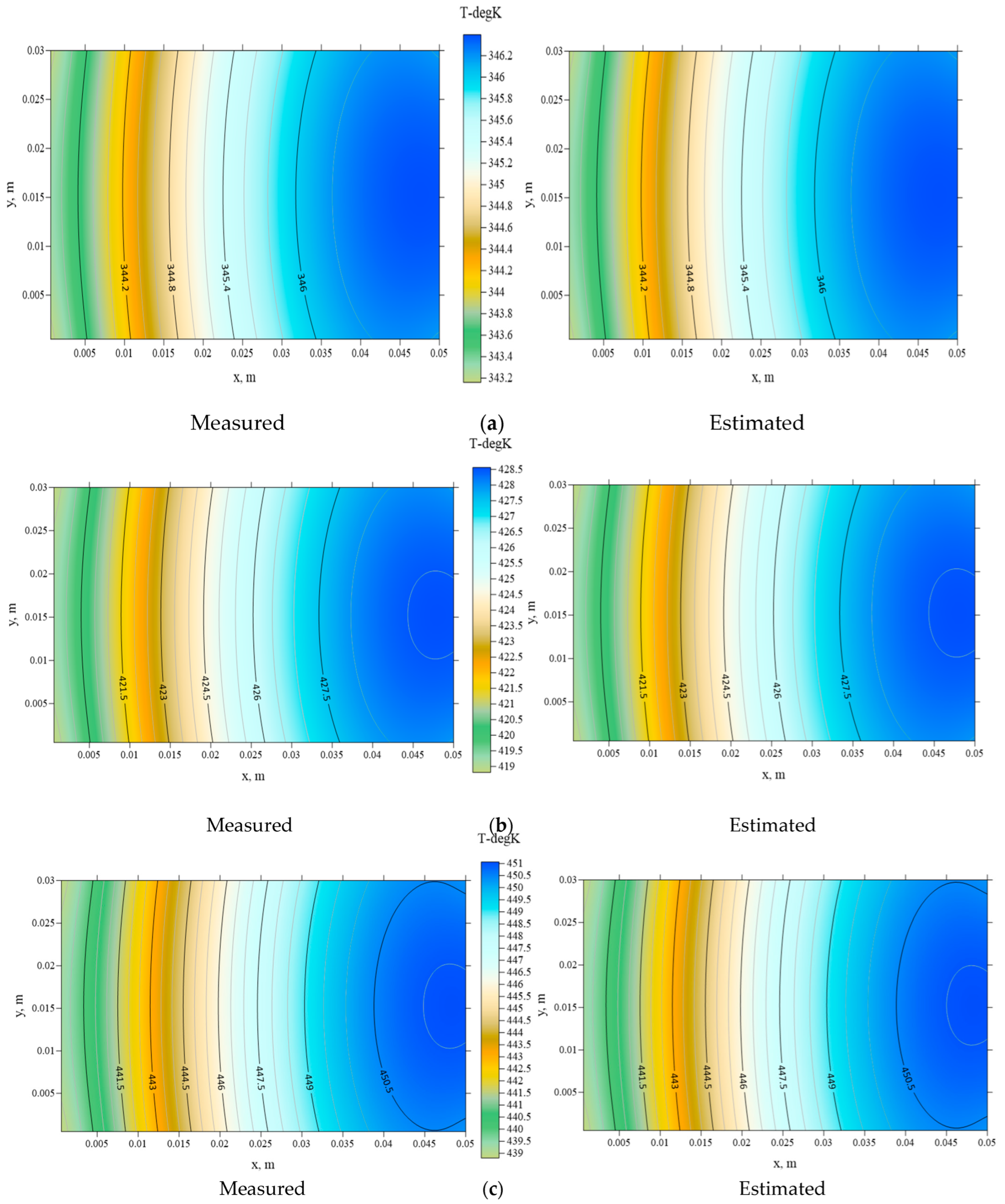
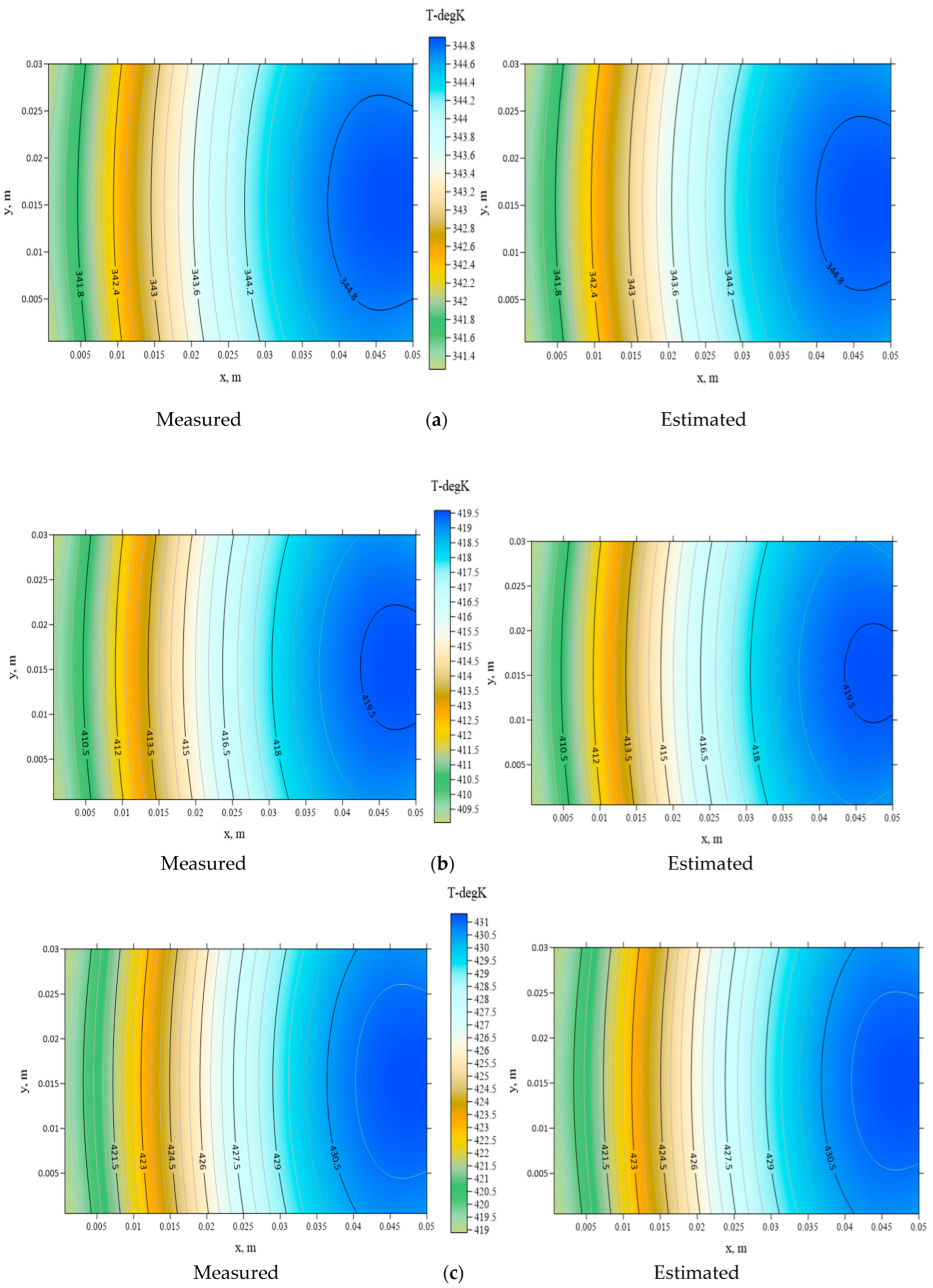
The corresponding measured Y(Stop,t) and estimated T(Stop,t) temperatures are presented in Figure 4a–c at t = 15, 45, and 80 s, respectively. From Figure 4, it is evident that the measured and estimated temperatures are nearly identical, suggesting the validity of the inverse algorithm for the present inverse conjugate heat transfer problem. The computed errors were ERR1 = 0.001% and ERR2 = 0.17% when σ = 0.0.
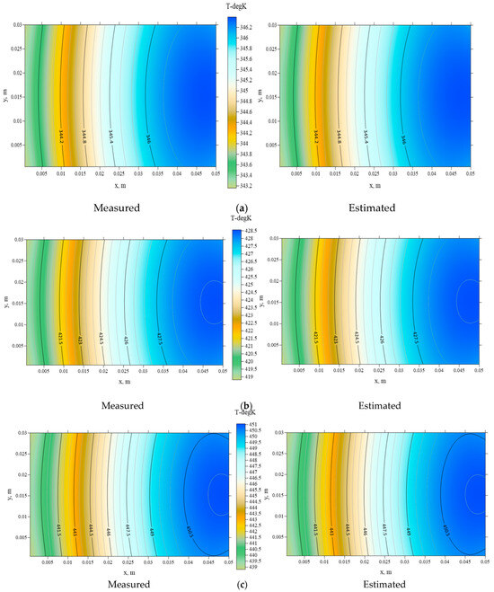
Figure 4.
The 2-D plots of measured and estimated temperatures over Stop at t = (a) 15, (b) 45, and (c) 80 s when σ = 0, Lz = 1 mm, and uin = 5 m/s in Example 1.
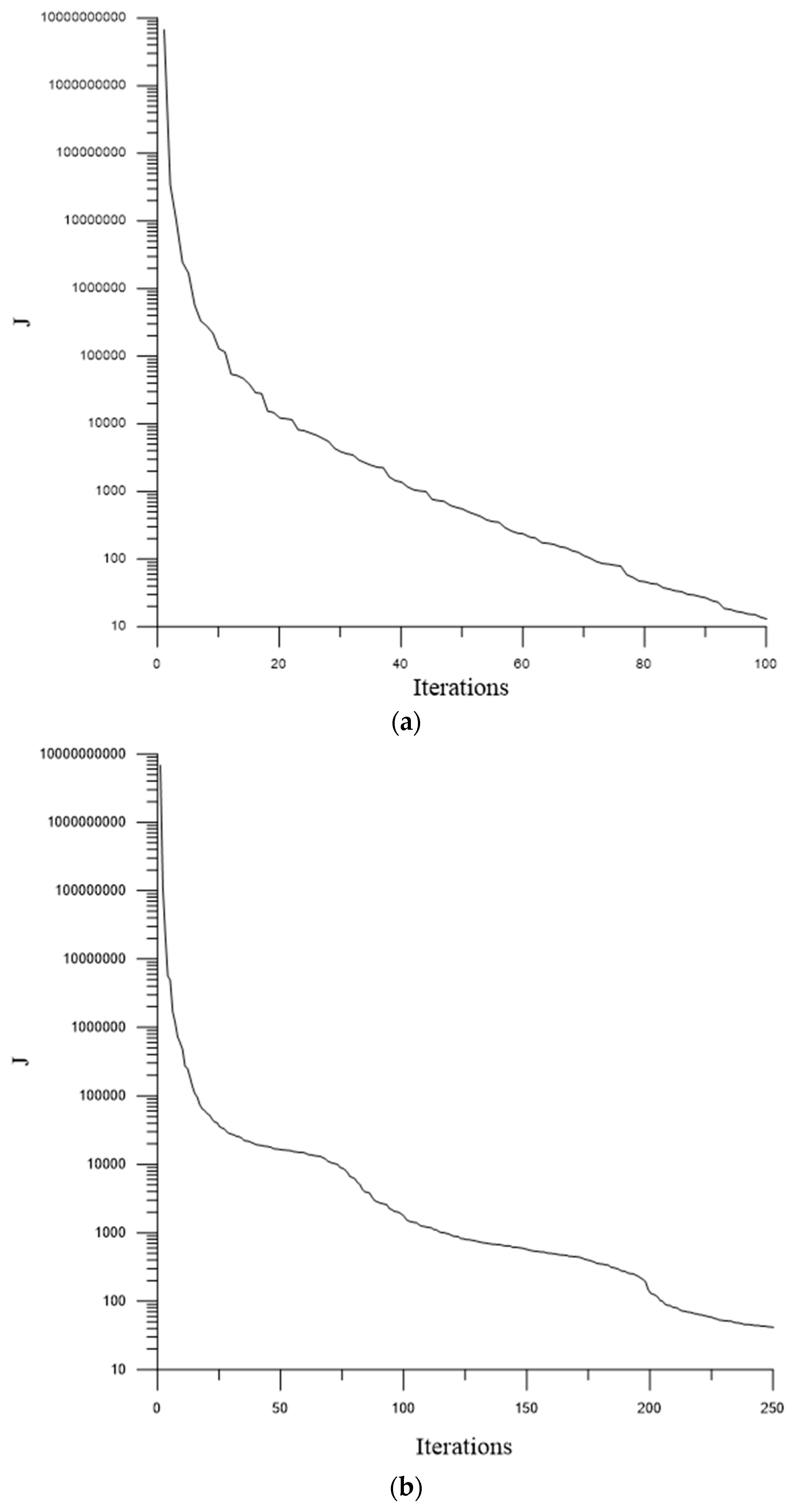
Figure 5a illustrates the cost function versus the iteration numbers, demonstrating a decrease from 6,734,652,281 to 13 after 100 iterations. This trend suggests that the estimated q(Sbottom,t) rapidly converges towards the exact q(Sbottom,t) globally using the CGM, as the convergent speed is very rapid over the initial iterations. Subsequently, the remaining iterations are utilized to fine-tune the estimated q(Sbottom,t) locally.

Figure 5.
The rate of convergence in (a) Example 1 and (b) Example 2 when uin = 5 m/s, Lz = 1 mm, and σ = 0.
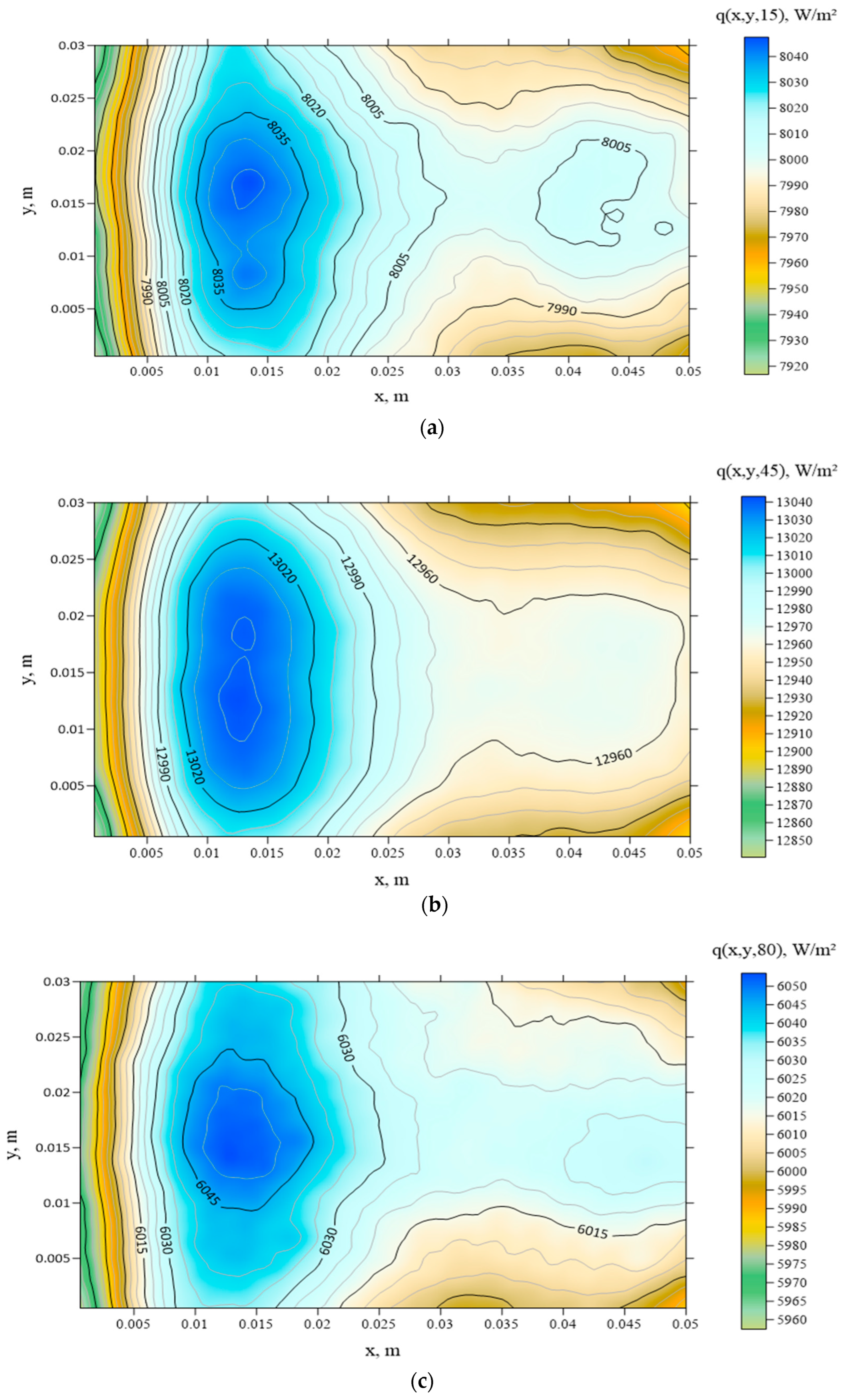
Here, the investigation focuses on the primary concern of how inexact temperature measurements impact the estimation of heat flux in inverse problems. Initially, the measurement error is set to σ = 0.05, and then it is increased to σ = 0.1. The convergent criterion ε is obtained with Equation (33), and the estimated q(Sbottom,t) is obtained after 60 and 44 iterations. The average errors ERR1 and ERR2 are 0.009% and 0.5% for σ = 0.05, respectively, and 0.019% and 0.92% for σ = 0.1, respectively. The 2-D plots of the estimated q(Sbottom,15), q(Sbottom,45) and q(Sbottom,80) are shown in Figure 6a–c for σ = 0.1. These findings suggest that the reliability of heat flux estimation persists even when utilizing inexact measurements.

Figure 6.
The 2-D plots of the estimated heat fluxes over Sbottom at t = (a) 15, (b) 45, and (c) 80 s when σ = 0.1, Lz = 1 mm, and uin = 5 m/s in Example 1.
Once again, the estimated q(Sbottom,t) values when σ = 0.05 and 0.1 at (0.025 m, 0.015 m, 0.0 m) for (a) 0 < t < 100, (b) 0 < t < 30, (c) 30 < t < 60, and (d) 60 < t < 100 s are plotted in Figure 3a,d, respectively. It is noticeable that the oscillation behaviors of the estimated heat flux become more pronounced near the discontinuity region as the measurement error is increased.
To explore the impact of the inlet air velocity on the estimated results and confirm the effectiveness of the proposed algorithm, we elevated the air velocity to uin = 8 m/s for Lz = 1 mm when σ = 0, 0.05, and 0.1. The corresponding iteration numbers, cost function J, and ERR1 and ERR2 values are presented in Table 1. The values of ERR1 and ERR2 are 0.0007% and 0.16% for σ = 0.0, 0.009% and 0.53% for σ = 0.05, and 0.02% and 0.93% for σ = 0.1, respectively. The 2-D plots of the q(Sbottom,15), q(Sbottom,45), when q(Sbottom,80) are illustrated in Figure 7a–c, respectively, and the measured temperatures Y(Stop,15), Y(Stop,45), and Y(Stop,80) and estimated the temperatures T(Stop,15), T(Stop,45), and T(Stop,80) are given in Figure 8a–c, respectively, when σ = 0.1.

Table 1.
The estimated results with different operational conditions for Examples 1 and 2.

Figure 7.
The 2-D plots of the estimated heat fluxes over Sbottom at t = (a) 15, (b) 45, and (c) 80 s when σ = 0.1, Lz = 1 mm, and uin = 8 m/s in Example 1.

Figure 8.
The 2-D plots of measured and estimated temperatures over Stop at t = (a) 15, (b) 45, and (c) 80 s when σ = 0.1, Lz = 1 mm, and uin = 8 m/s for Example 1.
A comparison of these figures demonstrates a remarkable similarity between the estimated values of q(Sbottom, t) over Sbottom for uin = 5 and 8 m/s. These findings imply that for laminar flow, the air velocity exerts a negligible influence on the inverse solutions.
(B) Example 2
The assumed functional form of the q(Sbottom,t) now takes the following expression:
This representation corresponds to a combination of sine and cosine functions, providing a thorough examination of the inverse algorithm due to the complexity of the spatially and temporally varying heat flux functions. Example 2 was used to verify the CGM’s capability of accurately estimating the defined heat fluxes.
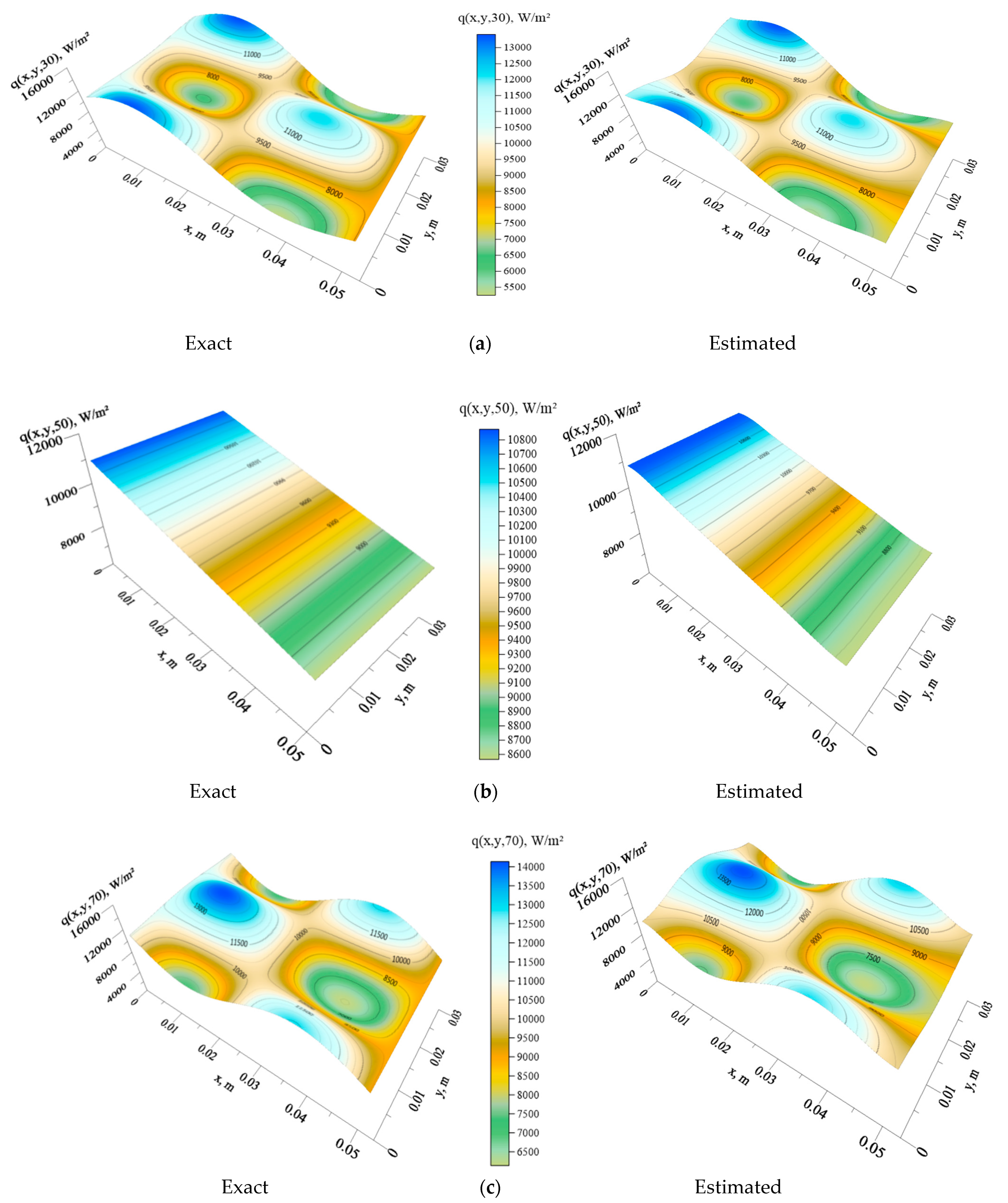
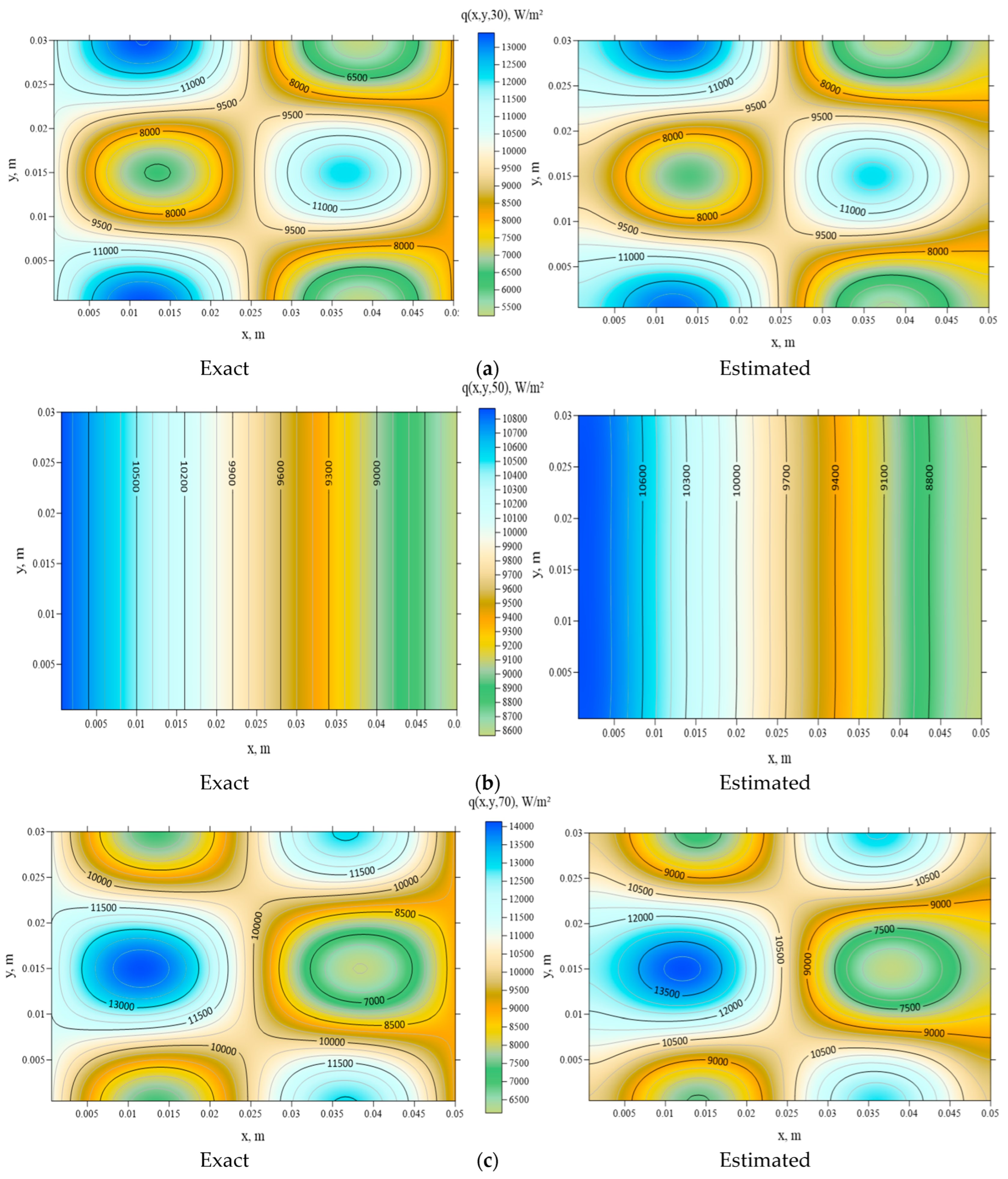
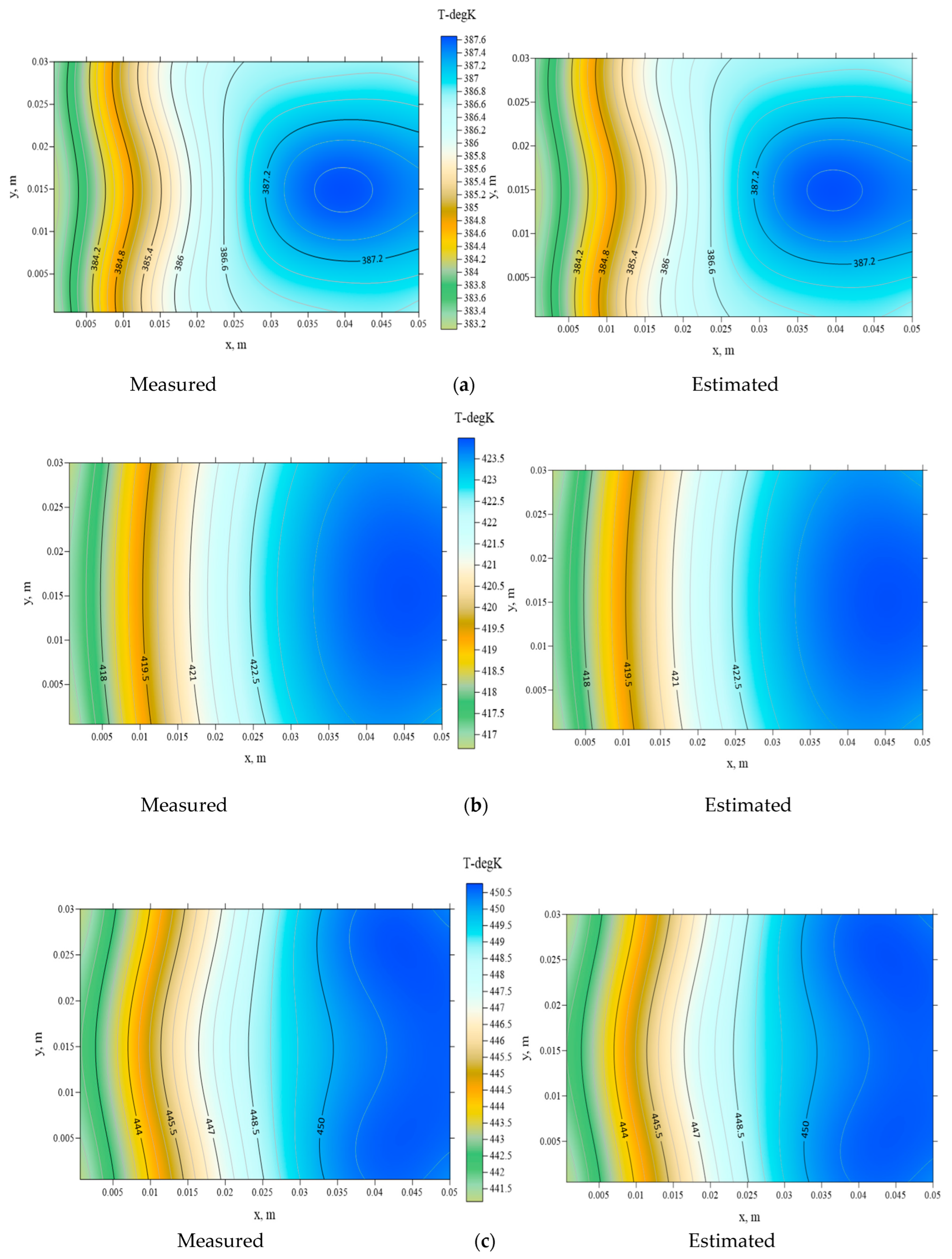
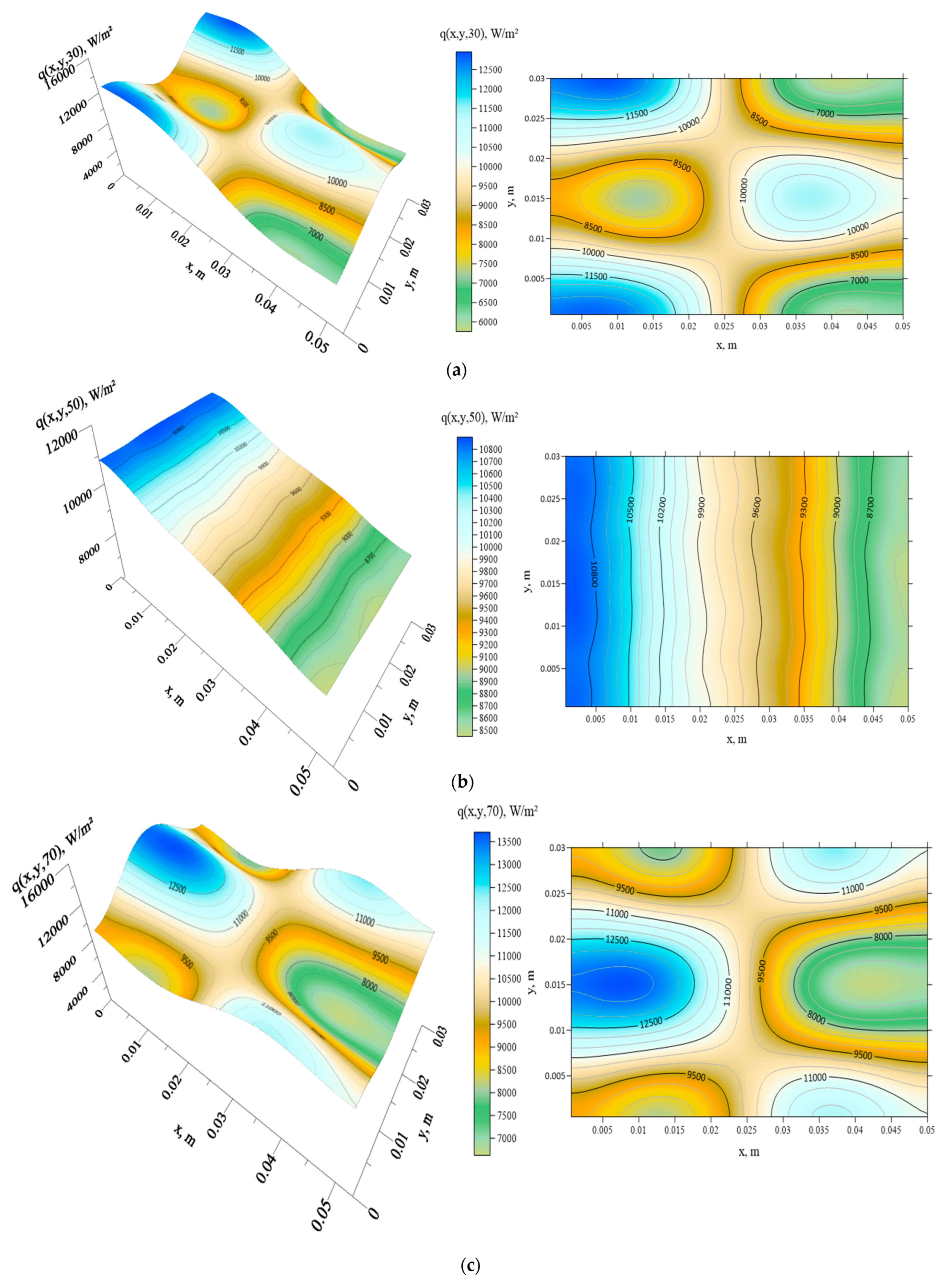
The 3-D and 2-D plots for the exact q(Sbottom,30), q(Sbottom,50), and q(Sbottom,70) are illustrated in Figure 9 and Figure 10, respectively, while the 2-D plots of the exact measured temperatures Y(Stop,30), Y(Stop,50), and Y(Stop,70) based on the exact q(Sbottom,t) value are given in Figure 11.

Figure 9.
The 3-D plots of the exact and estimated heat fluxes over Sbottom at t = (a) 30, (b) 50, and (c) 70 s when σ = 0, Lz = 1 mm, and uin = 5 m/s in Example 2.

Figure 10.
The 2-D plots of the exact and estimated heat fluxes over Sbottom at t = (a) 30, (b) 50, and (c) 70 s when σ = 0, Lz = 1 mm, and uin = 5 m/s in Example 2.
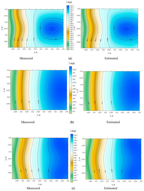
Figure 11.
The 2-D plots of measured and estimated temperatures over Stop at t = (a) 30, (b) 50, and (c) 70 s when σ = 0, Lz = 1 mm, and uin = 5 m/s in Example 2.
The inverse algorithm is then executed when σ = 0, Lz = 1 mm, and uin = 5 m/s. The functional J exhibits a rapid convergence rate within the initial iterations, diminishing to 42 after 250 iterations. The predicted 3-D and 2-D contour plots of q(Sbottom,30), q(Sbottom,50), and q(Sbottom,70) are presented in Figure 9 and Figure 10, respectively, and the estimated T(Stop,30), T(Stop,50), and T(Stop,70) values are presented in Figure 11. The values of ERR1 and ERR2 were computed to be 0.001% and 1.29%, respectively.
Based on the plotted figures and calculated errors, it can be concluded that the estimation of heat flux using the CGM is highly accurate, even when the considered function of the spatially distributed heat flux is very complex.
In Figure 5b, the cost function is plotted against the number of iterations using exact measurements, showing a decrease from 6,999,812,239 to 42 over 250 iterations. This outcome underscores the rapid convergence of the estimated q(Sbottom,t) towards the exact global q(Sbottom,t) during the initial iterations, while the subsequent iterations focus on refining the estimated q(Sbottom,t) locally.
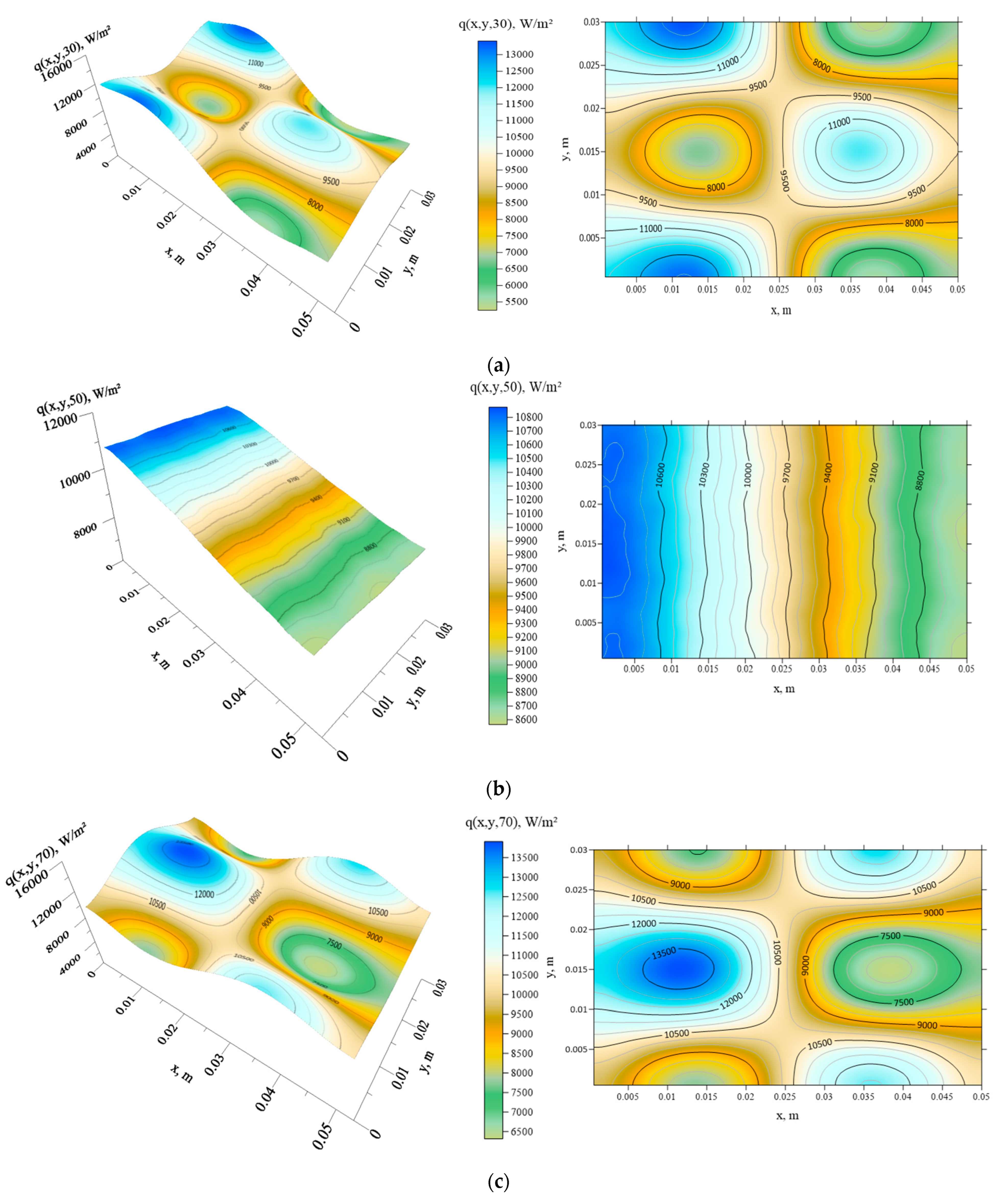
Next, the noise data are increased to σ = 0.05. The estimated q(Sbottom,t) is obtained after 182 iterations, and the 3-D and 2-D plots of the estimated q(Sbottom,30), q(Sbottom,50), and q(Sbottom,70) values are shown in Figure 12. The values of ERR1 and ERR2 were 0.01% and 2.45%, respectively.

Figure 12.
The 3-D and 2-D plots of the estimated heat fluxes over Sbottom at t = (a) 30, (b) 50 and, (c) 70 s when σ = 0.05, Lz = 1 mm, and uin = 5 m/s in Example 2.
This result underscores the reliability of the estimated heat fluxes even in the presence of measurement errors. However, when the measurement error is increased to σ = 0.1, the estimations become less accurate. This suggests that when the shape of the spatially distributed heat flux becomes more complex, more precise measurement data are necessary to achieve accurate estimations.
Next, we delve into the examination of how wall thickness affects the estimated heat flux. The inverse algorithm is used, with σ = 0 and 0.05 for Lz = 2 mm and uin = 5 m/s. When σ = 0, the cost function decreases to 65 after 250 iterations, and the values of ERR1 and ERR2 are calculated to be 0.002% and 2.99%, respectively. When σ = 0.05, J decreases to 1193 after 143 iterations, and ERR1 and ERR2 are 0.01% and 5.19%, respectively. They are reported in Table 1. The estimated 3-D and 2-D plots of the heat fluxes q(Sbottom,30), q(Sbottom,50), and q(Sbottom,70) are shown in Figure 13. Again, the estimation remains reliable for Lz = 2 mm but is less accurate compared to the case for Lz = 1 mm.

Figure 13.
The 3-D and 2-D plots of the estimated heat fluxes over Sbottom at t = (a) 30, (b) 50, and (c) 70 s when σ = 0.05, Lz = 2 mm, and uin = 5 m/s in Example 2.
Drawing from the outcomes of the two test examples outlined previously, it can be inferred that the spatially and temporally dependent surface heat flux q(Sbottom,t), in an inverse conjugate heat transfer scenario, has been precisely estimated. The function estimation retained its reliability whether exact or inexact temperature measurements were employed, particularly in cases of thin walls.
6. Conclusions
The successful resolution of a three-dimensional inverse conjugate heat transfer problem was achieved in order to estimate unknown temporally and spatially dependent boundary heat fluxes, using a thermal camera to perform thermography techniques. The conjugate gradient method (CGM) was chosen as the optimization algorithm due to its capability to handle function estimation problems without the need to assume a specific functional form for the heat flux, and the initial guesses for the inverse solutions were assumed arbitrarily. While the CGM was previously employed in solving inverse heat conduction, convection, or radiation problems, its application to inverse conjugate heat transfer problems has not been explored until now.
Various test cases were examined, encompassing different functional forms of heat fluxes, plate thicknesses, inlet velocities, and measurement errors. The simulation outcomes revealed that the CGM-derived estimates of the heat fluxes remained dependable even with increasing inlet air velocities and measurement errors under thin-wall conditions (i.e., Lz = 1 or 2 mm). Notably, when σ = 0, the maximum errors of ERR1 and ERR2 were found to be less than 0.001% and 0.17%, respectively, in Example 1, and less than 0.002% and 2.99%, respectively, in Example 2. It was also noted that smaller measurement errors were necessary when estimating the complex heat flux function in Example 2 to achieve the same level of accuracy required for both Examples 1 and 2. Additionally, the mitigation of poor estimations near the final time point caused by the singularity of the cost function gradient at tf can be achieved by extending the measurement duration.
The numerical experiments conducted led to the conclusion that CFD-ACE+ is a highly effective computational tool for resolving the addressed three-dimensional inverse conjugate heat transfer problem, enabling the determination of unknown surface heat fluxes through the CGM. When accounting for non-ideal thermal contact conditions, thermal contact conductance arises, resulting in additional heat losses. By detecting and incorporating these heat losses into thermography techniques, achieving precise estimations of heat flux becomes feasible.
The proposed algorithm holds promise for applications in numerous practical three-dimensional inverse engineering problems, thereby offering a versatile and reliable solution.
Author Contributions
Methodology, C.-H.H.; Software, K.-C.F.; Validation, C.-H.H.; Formal analysis, C.-H.H.; Investigation, K.-C.F.; Resources, C.-H.H.; Data curation, K.-C.F.; Writing—original draft, K.-C.F.; Writing—review & editing, C.-H.H.; Visualization, C.-H.H.; Supervision, C.-H.H.; Funding acquisition, C.-H.H. All authors have read and agreed to the published version of the manuscript.
Funding
This work was supported in part through the National Science and Technology Council, Taiwan, Grant number NSTC-112-2221-E-006-140-MY3.
Data Availability Statement
Data are contained within the article.
Conflicts of Interest
The authors declare no conflict of interest.
References
- Asif, M.; Tariq, A.; Singh, K.M. Estimation of thermal contact conductance using transient approach with inverse heat conduction problem. Heat Mass Transf. 2019, 55, 3243–3264. [Google Scholar] [CrossRef]
- Bozzoli, F.; Cattani, L.; Mocerino, A.; Rainieri, S.; Bazán, F.S.V. A novel method for estimating the distribution of convective heat flux in ducts: Gaussian filtered singular value decomposition. Inverse Probl. Sci. Eng. 2019, 27, 1595–1607. [Google Scholar] [CrossRef]
- Cui, M.; Mei, J.; Zhang, B.-W.; Xu, B.-B.; Zhou, L.; Zhang, Y. Inverse identification of boundary conditions in a scramjet combustor with a regenerative cooling system. Appl. Therm. Eng. 2018, 134, 555–563. [Google Scholar] [CrossRef]
- Guo, Z.; Lu, T.; Liu, B. Inverse heat conduction estimation of inner wall temperature fluctuations under turbulent penetration. J. Therm. Sci. 2017, 26, 160–165. [Google Scholar] [CrossRef]
- Kostin, A.B. Counterexamples in inverse problems for parabolic, elliptic, and hyperbolic equations. Comput. Math. Math. Phys. 2014, 54, 797–810. [Google Scholar] [CrossRef]
- Ku, C.-Y.; Xiao, J.-E.; Huang, W.-P.; Yeih, W.; Liu, C.-Y. On Solving Two-Dimensional Inverse Heat Conduction Problems Using the Multiple Source Meshless Method. Appl. Sci. 2019, 9, 2629. [Google Scholar] [CrossRef]
- Lukyanenko, D.; Yeleskina, T.; Prigorniy, I.; Isaev, T.; Borzunov, A.; Shishlenin, M. Inverse Problem of Recovering the Initial Condition for a Nonlinear Equation of the Reaction–Diffusion–Advection Type by Data Given on the Position of a Reaction Front with a Time Delay. Mathematics 2021, 9, 342. [Google Scholar] [CrossRef]
- Al-Mahdawi, H.K.I.; Abotaleb, M.; Alkattan, H.; Tareq, A.Z.; Badr, A.; Kadi, A. Multigrid Method for Solving Inverse Problems for Heat Equation. Mathematics 2022, 10, 2802. [Google Scholar] [CrossRef]
- Mohebbi, F. Function Estimation in Inverse Heat Transfer Problems Based on Parameter Estimation Approach. Energies 2020, 13, 4410. [Google Scholar] [CrossRef]
- Naveira-Cotta, C.P.; Cotta, R.M.; Orlande, H.R.B. Inverse analysis of forced convection in micro-channels with slip flow via integral transforms and Bayesian inference. Int. J. Therm. Sci. 2010, 49, 879–888. [Google Scholar] [CrossRef]
- Rothermel, D.; Schuster, T. Solving an inverse heat convection problem with an implicit forward operator by using a projected quasi-Newton method. Inverse Probl. 2021, 37, 045014. [Google Scholar] [CrossRef]
- VanderVeer, J.R.; Jaluria, Y. Solution of the inverse jet in a crossflow problem by a predictor–corrector technique. Int. J. Heat Mass Transf. 2015, 89, 929–936. [Google Scholar] [CrossRef]
- VanderVeer, J.R.; Jaluria, Y. Solution of an inverse convection problem by a predictor–corrector approach. Int. J. Heat Mass Transf. 2013, 65, 123–130. [Google Scholar] [CrossRef]
- Prud’homme, M.; Nguyen, T.H. Solution of inverse free convection problems by conjugate gradient method: Effects of Rayleigh number. Int. J. Heat Mass Transf. 2001, 44, 2011–2027. [Google Scholar] [CrossRef]
- VanderVeer, J.R.; Jaluria, Y. Optimization of an inverse convection solution strategy. Int. J. Heat Mass Transf. 2014, 73, 664–670. [Google Scholar] [CrossRef]
- Bangian-Tabrizi, A.; Jaluria, Y. An optimization strategy for the inverse solution of a convection heat transfer problem. Int. J. Heat Mass Transf. 2018, 124, 1147–1155. [Google Scholar] [CrossRef]
- Liu, D.; Wang, F.; Yan, J.H.; Huang, Q.X.; Chi, Y.; Cen, K.F. Inverse radiation problem of temperature field in three-dimensional rectangular enclosure containing inhomogeneous, anisotropically scattering media. Int. J. Heat Mass Transf. 2008, 51, 3434–3441. [Google Scholar] [CrossRef]
- Liu, L.H.; Tan, H.P.; Yu, Q.Z. Inverse radiation problem of sources and emissivities in one-dimensional semitransparent media. Int. J. Heat Mass Transf. 2001, 44, 63–72. [Google Scholar] [CrossRef]
- Park, H.M.; Yoon, T.Y. Solution of the inverse radiation problem using a conjugate gradient method. Int. J. Heat Mass Transf. 2000, 43, 1767–1776. [Google Scholar] [CrossRef]
- Wen, S.; Qi, H.; Ren, Y.-T.; Sun, J.-P.; Ruan, L.-M. Solution of inverse radiation-conduction problems using a Kalman filter coupled with the recursive least–square estimator. Int. J. Heat Mass Transf. 2017, 111, 582–592. [Google Scholar] [CrossRef]
- Huang, C.H.; He, K.-J. A Steady-State Inverse Heat Conduction-Convection Conjugated Problem in Determining Unknown Spatially Dependent Surface Heat Flux. Case Stud. Therm. Eng. 2022, 39, 102411. [Google Scholar] [CrossRef]
- Huang, C.H.; He, K.-J. An Experimental Inverse Problem in Determining Spatially Varying Surface Heat Flux Using Measured Temperature Readings. Case Stud. Therm. Eng. 2023, 49, 103227. [Google Scholar] [CrossRef]
- Alifanov, O.M. Inverse Heat Transfer Problems; Springer: Berlin/Heidelberg, Germany, 1994. [Google Scholar]
- Zhou, J.; Zhang, Y.; Chen, J.K.; Feng, Z.C. Inverse estimation of surface heating condition in a three-dimensional object using conjugate gradient method. Int. J. Heat Mass Transf. 2010, 53, 2643–2654. [Google Scholar] [CrossRef]
- Huang, C.H.; Wang, S.P. A Three-Dimensional Inverse Heat Conduction Problem in Estimating Surface Heat Flux by Conjugate Gradient Method. Int. J. Heat Mass Transf. 1999, 42, 3387–3403. [Google Scholar] [CrossRef]
- Huang, C.H.; Chen, W.C. A Three-Dimensional Inverse Forced Convection Problem in Estimating Surface Heat Flux by Conjugate Gradient Method. Int. J. Heat Mass Transf. 2000, 43, 3171–3181. [Google Scholar] [CrossRef]
- Zhang, C.; Li, B.-W.; Zhou, R.-R.; Li, P.-X.; Huang, L.-Y. Inverse analysis of radiative properties of internal medium and surface for cylindrical system using CSM-CGM approach. Int. J. Therm. Sci. 2023, 190, 108329. [Google Scholar] [CrossRef]
- CFD-ACE+ User’s Manual, ESI-CFD Inc.: Bagnuex, France, 2020.
- IMSL by Perforce©, Perforce Software, Inc.: Minneapolis, USA, 2021.
Disclaimer/Publisher’s Note: The statements, opinions and data contained in all publications are solely those of the individual author(s) and contributor(s) and not of MDPI and/or the editor(s). MDPI and/or the editor(s) disclaim responsibility for any injury to people or property resulting from any ideas, methods, instructions or products referred to in the content. |
© 2024 by the authors. Licensee MDPI, Basel, Switzerland. This article is an open access article distributed under the terms and conditions of the Creative Commons Attribution (CC BY) license (https://creativecommons.org/licenses/by/4.0/).

