Article

A Mathematical Analysis of Competitive Dynamics and Aggressive Treatment in the Evolution of Drug Resistance in Malaria Parasites

1
School of Economics and Management, Shanghai Maritime University, Shanghai 201306, China
2
Shanghai Institute of Aerospace System Engineering, Shanghai 201108, China
*
Author to whom correspondence should be addressed.
Mathematics 2024, 12(10), 1595; https://doi.org/10.3390/math12101595
Submission received: 24 April 2024 / Revised: 15 May 2024 / Accepted: 18 May 2024 / Published: 20 May 2024

Abstract

:
Experimental evidence supports the counterintuitive notion that rapid eradication of pathogens within a host, infected with both drug-sensitive and -resistant malaria parasites, can actually accelerate the evolution of drug-resistant pathogens. This study aims to analyze the competitive dynamics between these two strains through a mathematical model and evaluate the impact of aggressive treatment on the spread of drug resistance. We conducted equilibrium, uncertainty, and sensitivity analyses to assess the model, identifying and measuring the influence of key factors on the outcome variable (the population of drug-resistant parasites). Both equilibrium and local sensitivity analyses concurred that the density of drug-resistant parasites is notably affected by genetic instability, the production rate of red blood cells, the number of merozoites, and competition factors. Conversely, there is a negative relationship between genetic instability and one of the competition coefficients. Global sensitivity analysis offers a comprehensive examination of the impact of each input parameter on the temporal propagation of drug resistance, effectively accounting for the interplay among parameters. Both local and global sensitivity analyses underscore the continuous impact of drug treatment on the progression of drug resistance over time. This paper anticipates exploring the underlying mechanisms of drug resistance and providing theoretical support for developing more effective drug treatment strategies.

1. Introduction

Drug resistance in malaria refers to the ability of strains of Plasmodium parasites to persist and reproduce even when exposed to recommended or higher doses of antimalarial drugs [1]. This resistance arises due to the widespread use of common antimalarial medications, leading to resistance in severe forms of the disease. Despite intensified efforts for control, progress towards malaria elimination has stalled in recent years [2,3]. The World Health Organization has recommended several artemisinin-based combination therapies (ACTs) for the treatment of uncomplicated falciparum malaria [4]. While ACTs have significantly reduced malaria morbidity and mortality rates globally, the challenge of drug resistance persists, particularly in regions such as Southeast Asia [5], South America [6], Papua New Guinea [7], and Eastern Africa [8].
In theory, drug treatment is a crucial intervention for patients infected with malaria, as it can alleviate symptoms and reduce mortality rates. However, during drug treatment, sensitive parasites are typically eliminated. If the concentration achieved is insufficient to kill all drug-resistant mutants, populations of surviving resistant mutants will rapidly expand, enabling their survival and reproduction [9]. This scenario increases the likelihood of drug resistance spreading to the next generation, potentially leading to its widespread prevalence. Importantly, experimental evidence suggests that, when an aggressive treatment regimen is employed, sensitive parasites are swiftly eradicated, potentially giving a competitive advantage to drug-resistant parasites [10,11,12]. Therefore, the competition between sensitive and drug-resistant parasites is crucial in this context [13,14,15]. In contrast, a more moderate treatment approach allows some sensitive parasites to persist and compete with drug-resistant strains, thereby suppressing the latter and delaying the onset of resistance [16]. Based on this analysis, it is evident that drug treatment plays a pivotal role in influencing the development of drug resistance. Consequently, there is an urgent need to explore the relationship between drug-resistant parasites and drug concentration, which is a topic of paramount importance.
Mathematical modeling is considered a crucial tool for understanding the evolution of drug resistance. This tool not only elucidates interactions between different parasite strains, but also provides a theoretical foundation for managing resistance. In recent years, various epidemiological models have emerged for studying drug-resistant parasites. One study indicated that high transmission intensity may hinder the evolution of resistance by affecting host population immunity [17]. Similarly, another study found that early transmission of drug-sensitive parasites and asymptomatic infections can delay the onset of drug resistance [18]. Additionally, models have focused on the relative size of the host population infected with resistant parasites and its impact on the spread of drug resistance [19]. Mathematical models for malaria have integrated treatment and varying levels of resistance to analyze the role of treatment in the development of drug resistance [20]. Concurrently, research has investigated the potential contribution of co-infection competitive release to the emergence of resistance [21]. While some studies aim to devise optimal strategies for controlling resistance spread through model analysis, research simultaneously addressing drug treatment and competition is relatively scarce [22,23]. Therefore, it is necessary to construct a comprehensive model that integrates these key elements and draws upon experimental findings from multiple sources [15,16,24].
One of the primary objectives of this paper is to identify influential factors and explore the relationship between the density of drug-resistant parasites and input parameters. Typically, this goal can be achieved by directly computing the mathematical expression representing the state variable of drug-resistant parasites in our model. However, due to the complexity of our model, deriving a specific formulation for the state variable of drug-resistant parasites proves to be a challenging task. Consequently, we are compelled to seek alternative approaches. Uncertainty and sensitivity analyses serve as important tools for gaining insights into the mechanisms governing system behaviors. In particular, uncertainty analysis helps quantitatively assess biases in the results of epidemiological studies, enhancing our understanding of the inherent uncertainties in the data and methodologies used [25]. By conducting sensitivity analysis, we can not only identify the parameters significantly influencing the outcome variables of interest, but also quantify how input uncertainties impact the overall results of the model [26].
This paper focuses on a thorough investigation of the model proposed in [27], which considers the dynamics of drug treatment and within-host competition between drug-sensitive and drug-resistant parasites. Built upon empirical observations [15,16,24], these observations highlight a counterintuitive phenomenon: rapid pathogen clearance in a host co-infected with both drug-sensitive and drug-resistant malaria parasites may paradoxically accelerate the emergence of drug resistance. This paradox arises from the competitive interactions between the two parasite strains. To validate and refine the model, we aligned it with experimental data to facilitate parameter estimation for subsequent statistical analysis. Subsequently, we conducted a series of analytical procedures, including uncertainty analysis, local sensitivity analysis, and global sensitivity analysis, to investigate the behavior of the model under various conditions. We particularly focused on the state variable representing the density of drug-resistant parasites, depicting it as a function of various input parameters through uncertainty analysis. Sensitivity analysis helps clarify how changes in the input parameters influence the evolution of drug resistance within the parameter space defined by the parameter ranges. In conclusion, the outcomes of this study hold the potential to provide insights for formulating optimal policies to manage drug resistance and control disease transmission.

2. Methods

2.1. Model

In this paper, we considered the model proposed in [27].
S ( t ) = Λ β 1 S I s β 2 S I r d 1 S , I s ( t ) = α β 1 S I s + p α β 2 S I r γ 1 I s I r ( d 2 + μ ) I s , I r ( t ) = ( 1 p ) α β 2 S I r γ 2 I s I r d 3 I r .
The model considers the dynamic changes in three distinct cell populations: uninfected red blood cells denoted as S ( t ) , drug-sensitive malaria parasites represented by I s ( t ) , and drug-resistant malaria parasites indicated as I r ( t ) . Uninfected red blood cells are continually supplied at a constant net rate Λ from the bone marrow and have a natural life expectancy of 1 / d 1 days. Malaria parasites infect red blood cells at a rate proportional to the contact rate associated with their population size. The transmission rates for the wild-type and drug-resistant parasites are denoted as β 1 and β 2 , respectively. Following a series of multiplication cycles, each infected red blood cell produces α infective merozoites (in the case of P. falciparum, each infected cell yields a substantial number of merozoites, typically ranging from 8 to 32 in humans). The parameter p represents the proportion of drug-sensitive parasites released from a red blood cell infected by a drug-resistant strain. The competition between the two parasite strains is characterized by the terms γ 1 I s ( t ) I s ( t ) and γ 1 I s ( t ) I s ( t ) , which align with the formulation used in numerous intra-host competition models. Both parasite strains experience mortality at per capita rates denoted as d 2 and d 3 . Additionally, the clearance rate of the wild-type strain is represented by μ .

2.2. Parameter Estimation

Parameter estimation was carried out within the dynamic framework of malaria infection, encompassing both competition and drug treatment. The model parameter values were estimated using the least squares method to fit a dataset on malaria infection from [24]. The least squares problem involves minimizing the discrepancy between the sum of squared differences and the observed data over a parameter vector space constrained by a predefined feasible region. It is crucial to recognize that the standard least squares formulation comprises two fundamental components: mathematical and statistical [28]. The mathematical model utilized in this study is the malaria model (1) we developed. The statistical model is built on the assumption that the output of the model and associated random deviations (measurement errors) are governed by the random variables:
Y j = I r ( t j ; θ ) + ϵ j , f o r j = 1 , , n ,
where θ = ( α , β 1 , β 2 , γ 1 , γ 2 , d 2 , d 3 , μ , p ) and I r ( t j ; θ ) denotes the output of the mathematical model (1). The random variables ϵ j model the random deviations away from I r ( t , θ ) and are assumed to satisfy that all ϵ j are independent and identically distributed random variables, E ( ϵ j ) = 0 for every j and v a r ( ϵ j ) = σ 2 < for every j. The objective function is given by
θ O L S = a r g m i n θ Θ j = 1 n ( Y j I r ( t j ; θ ) ) 2 ,
where θ O L S is the estimator, the set of parameter vectors θ constrained by a prespecified feasible region Θ . Θ is primarily determined based on the biological significance of the parameter. j represents the time point at which the time series data are observed, and n is the number of data points available for inference. Hence, the model solution I r ( t ; θ ) yields the best fit to the time series data Y j . The l s q c u r v e f i t function in Matlab 2015b (Mathworks, Inc., Natick, MA, USA) is used to find the least squares best fit to the data. Moreover, in Matlab, two numerical optimization methods are available to solve the nonlinear least squares problem: The trust-region-reflective algorithm and the Levenberg–Marquardt algorithm.

2.3. Equilibrium Analysis

In order to explore the relationship between the drug-resistant parasites and each parameter, computing the interior equilibrium is of primary importance. To determine the interior equilibrium of system (1), we denote P * = ( S * , I s * , I r * ) and let the right-hand side of (1) be zero. It then follows from the last two equations of (1) that
I s * = ( 1 p ) α β 2 S * d 3 γ 2
and
I r * = ( α β 1 S * d 2 μ ) [ ( 1 p ) α β 2 S * d 3 ] γ 1 [ ( 1 p ) α β 2 S * d 3 ] p α β 2 γ 2 S * .
Substituting I r * and I s * into the first equation of (1), we obtain the S * that satisfies
f ( S * ) : = k 1 S * 3 + k 2 S * 2 + k 3 S * + k 4 = 0 ,
where
k 1 = α 2 β 1 β 2 2 ( 1 p ) 2 ( γ 1 + γ 2 ) , k 2 = α β 2 ( 1 p ) [ 2 β 1 γ 1 d 3 + β 1 γ 2 d 3 + β 2 γ 2 ( d 2 + μ ) ] α β 2 γ 2 d 1 [ γ 1 ( 1 p ) p γ 2 ] , k 3 = Λ α β 2 γ 2 [ γ 1 ( 1 p ) p γ 2 ] β 1 γ 1 d 3 2 β 2 γ 2 d 3 ( d 2 + μ ) + γ 1 γ 2 d 1 d 3 , k 4 = Λ γ 1 γ 2 d 3 .
It is noteworthy that not all I r * values can keep positive due to the complex existence condition of I r * . According to Theorem 3 of [27], we can obtain the existence condition of the interior equilibrium P * . Model (1) also exhibits a fixed-point bifurcation. For details, please refer to Reference [27].
Theorem 1 
([27], Theorem 3). Assume that k 3 > 0 (or k 3 < 0 and k 2 > 0 ) and Δ : = k 2 2 3 k 1 k 3 > 0 . Then, (1) has two positive roots S ± * with S + * > S > S * , when f ( S ) > 0 . Moreover, the interior equilibrium exists by further assuming that S * (one of S ± * ) satisfies
( H 1 )
d 3 ( 1 p ) α β 2 < S * < min d 2 + μ α β 1 , γ 1 d 3 α β 2 ( γ 1 ( 1 p ) γ 2 p )  or
( H 2 )
max d 2 + μ α β 1 , d 3 ( 1 p ) α β 2 , γ 1 d 3 α β 2 ( γ 1 ( 1 p ) γ 2 p ) < S *

2.4. Uncertainty Analysis and Sensitivity Analysis Methods

2.4.1. Uncertainty Analysis

Uncertainty analysis was formally used to quantify the variability in the outcome variable, which was due to the uncertainty in estimating the values of the input parameters [29,30]. This type of analysis provides insight into the range of potential results that the model can generate. To initiate the uncertainty analysis, it was essential to define the prior distribution of the input parameters under consideration. Subsequently, a Latin Hypercube Sampling (LHS) method was applied. The outcomes were visualized through a histogram, shedding light on how the distribution changes when different assumptions and prior distributions for the bias parameters are altered [25]. To gain a comprehensive understanding of the outcome variable, various statistical measures such as the mean, variance, median, quantiles, and others were employed as valuable approaches.

2.4.2. Local Sensitivity Analysis (LSA)

Local sensitivity refers to the sensitivity of parameters with respect to a given parameter set, where only one parameter varies in a certain range and the other parameters are fixed. If the output variable y can be defined as follows:
y = f ( x ) = f ( x 1 , x 2 , , x n ) ,
where x = ( x 1 , x 2 , , x n ) represent the input parameters, the usual method to compute the sensitivity of the i-th input parameter on the outcome variable is by the partial derivative y x i at the nominal value of parameter x i . Derivative-based sensitivity analysis finds its rationale in the Taylor series expansion [31]. Note that it was hard to quantify the sensitivity if x i and y varied in different units of measurement; therefore, normalizing the sensitivity indices was necessary, which took the form:
S i = y x i σ x i σ y ,
where σ x i and σ y represent the standard deviation of input parameter x i and outcome variable y in Monte Carlo sampling, respectively. The normalized sensitivities of the model output are then given as
L 1 = | S i | / n , L 2 = ( S i 2 ) / n ;
L 1 and L 2 measure the impact of the input parameter on the model outcome variable to give a preference for tuning the parameter with a high sensitivity. Derivative-based sensitivity methods are widely performed due to the efficient calculations, but this also has the drawback that they provide information about local sensitivity only.

2.4.3. Global Sensitivity Analysis (GSA)

Compared to the local sensitivity analysis, GSA is performed over the entire parameter space, where all parameter variations are simultaneously considered. In addition, the interaction between the input parameters we are concerned with would be calculated. In this paper, we mainly apply the variance-based GSA method, i.e., the Sobol sensitivity method. The essence of Sobol sensitivity analysis is to measure sensitivity through variance decomposition [32,33]. According to Equation (6), x = ( x 1 , x 2 , , x n ) represent the input parameters, which are defined on an n-dimensional unit cube H n = x | 0 x i 1 , i = 1 , 2 , , n . Based on the Sobol method, y = f ( x ) can be decomposed into single model parameters and the subitem function of the parameter interaction:
f ( x ) = f 0 + i = 1 n f i ( x i ) + i = 1 n i j n f i j ( x i , x j ) + + f 1 , 2 , , n ( x 1 , x 2 , . , x n ) .
The number of all subitems is 2 n , and the subitem function is obtained by calculating the following multiple integrals:
f 0 = 0 1 f ( x ) d x , f i ( x i ) = 0 1 f ( x ) k i d x k f 0 , f i j ( x i , x j ) = 0 1 f ( x ) k i , j d x k f 0 f i ( x i ) f j ( x j ) .
Similarly, other subitem functions of high order can be achieved. f 0 is a constant, and the integral of every summand over any of its own variables is zero:
0 1 f i 1 , , i s ( x i 1 , , x i s ) d x k = 0 , 1 i 1 i 2 i s n , 1 s k .
The subitem functions in Equation (10) satisfy Equation (11), and it can be inferred that every subitem function in Equation (9) is orthogonal, which is:
H n f i 1 , , i s ( x i 1 , , x i s ) f j 1 , , j l ( x j 1 , , x j l ) d x = 0 , for ( x i 1 , , x i s ) ( x j 1 , , x j l ) .
Based on the above properties, the variance of output variable V ( y ) can be decomposed as follows:
V ( y ) = i = 1 n V i ( x i ) + i = 1 n i j n V i j ( x i , x j ) + + V 1 , 2 , , n ( x 1 , x 2 , , x n ) ,
where V i 1 , , i s = 0 1 f i 1 , , i s 2 ( x i 1 , , x i s ) d x i 1 , , x i s . is the partial variance corresponding to the subitem function of Equation (9). The Sobol global sensitivity indices are defined by
S i 1 , i 2 , , i s = V i 1 , i 2 , , i s V ( y ) .
We mainly considered first-order Sobol indices and total Sobol indices, which are
S i = V i V ( y ) ,
and
S T i = S i + S i j ( i j ) + + S 1 i s .
Equation (15) is the first-order Sobol index. Equation (16) is the total-order sensitivity index, as an extension of the Sobol sensitivity indices, which is defined as the ratio of the sum of the related sensitivity indices. Equations (15) and (16) explain the reason why the higher value of S i , the more importance of parameter x i on the outcome variable, but this is not applicable in reverse. In other words, a low value of the first-order index cannot necessarily stand for having no influence on the outcome variable due to the parameters’ interactions, which lead to a larger total-order index. Hence, total-order indices have a great significance. Parameter x i has no impact on the outcome variable in the case S T i = 0 and vice versa. In summary, first-order Sobol indices refer to the influence of each parameter on the outcome variable alone, which measure the importance of each parameter itself, whereas the total Sobol indices not only characterize the contribution of the concerned parameters, but also their interactions. The calculation of Sobol sensitivity indices involves the computation of multiple integrals, which is very complicated and difficult, especially for complex nonlinear models. Therefore, the Monte Carlo method is employed to approximate the multiple integral solution.

3. Results

3.1. Parameter Estimates

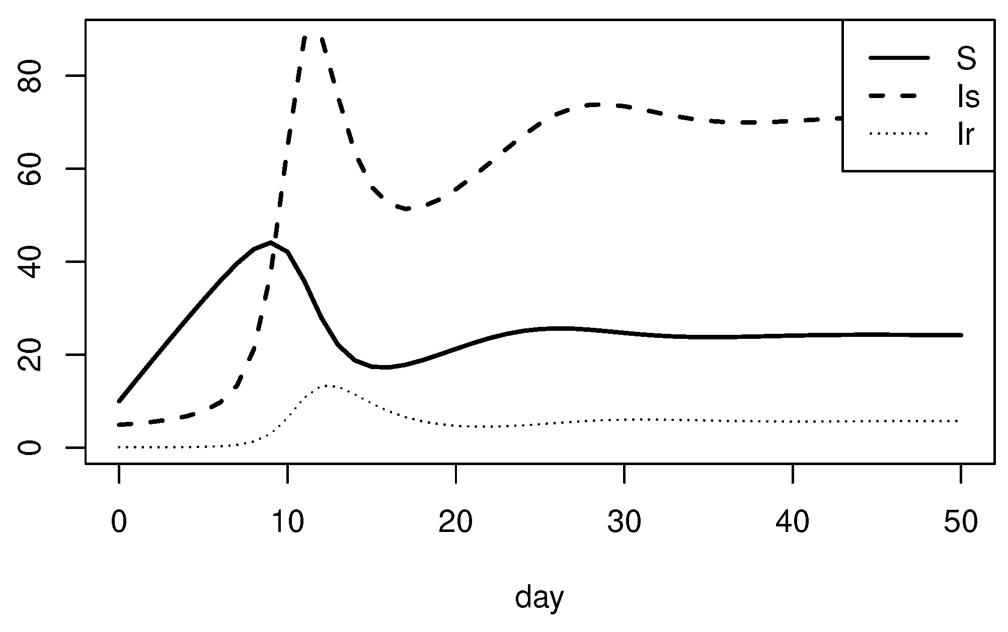
Optimal fits were obtained for the dataset in Figure 1. The model has a goodness-of-fit ratio R 2 = 0.9436 . In this paper, we fixed the parameter value of the production rate of RBCs ( Λ ) and the decay rate of RBCs ( d 1 ) based on the research of Anderson [34]. The estimated parameter values are shown in Table 1, where d 3 < d 2 accorded with the fact that the resistant mutants have a higher death rate than wild-type strains, reflecting the biological cost of resistance [19]. In addition, the solution curve was obtained on the basis of the parameter set we estimated (Figure 2), and the three cell populations involved in this model finally reached a steady state.

3.2. Equilibrium Analysis

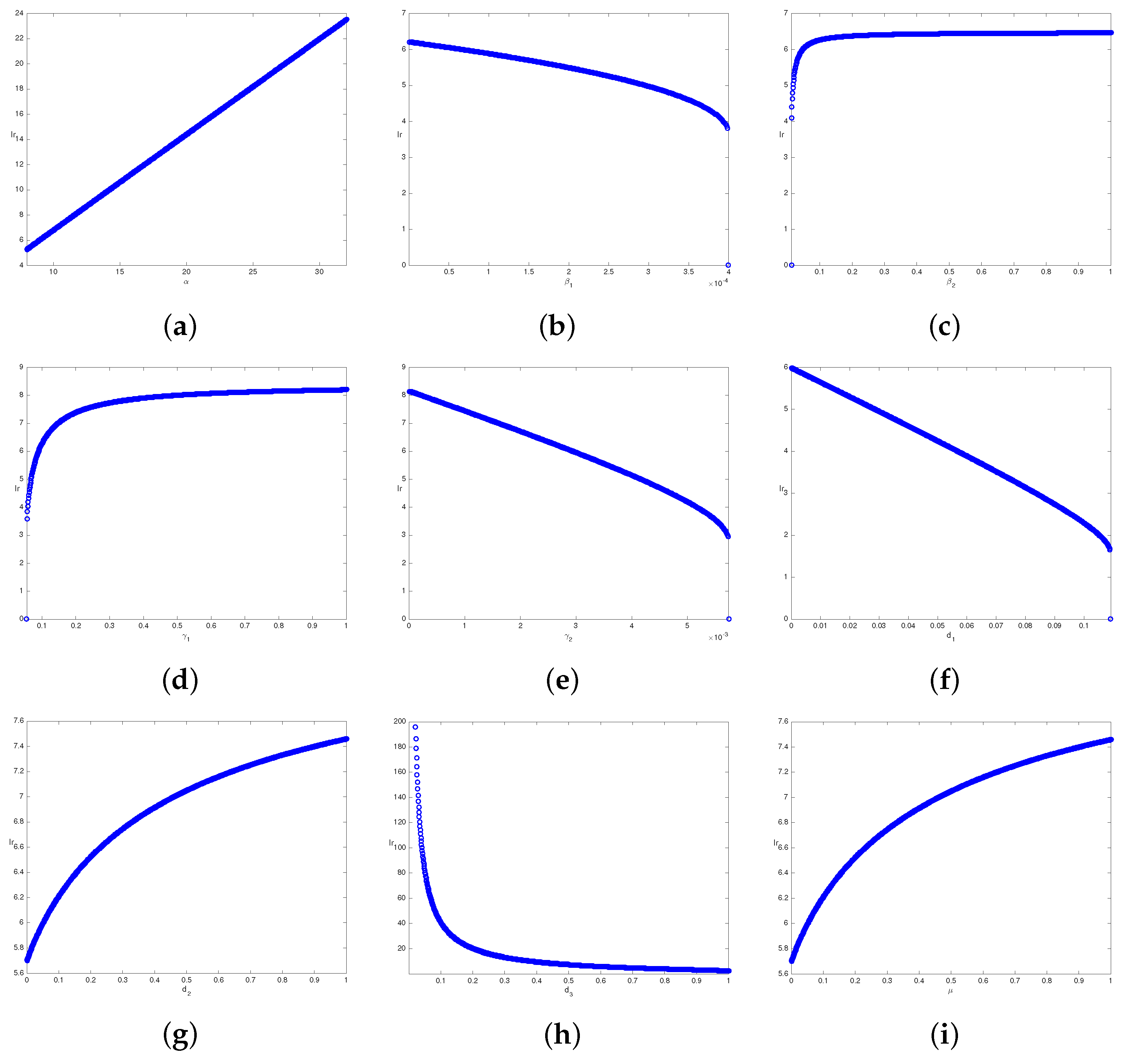
Equilibrium analysis is employed to observe the relationship between the parameters and the drug-resistant parasites in this paper. Calculating the interior equilibrium of the dynamical system is a necessary step, then we primarily focus on the part of I r in the equilibrium. Equilibrium analysis results are obtained in Figure 3. The results show a strong positive linearity between α and I r * as α varies in the interval [ 8 , 32 ] (Figure 3a), indicating the more merozoites were produced, the higher the value of I r * was. As the parameters β 1 and β 2 increase, I r * exhibits the tendency of decreasing and increasing, respectively (Figure 3b,c), but in general, their impact on I r * is not obvious, such that their effective intervals are much smaller. The trends of γ 1 (rising) and γ 2 (falling) on I r * are opposite, which exactly shows the importance of competition, that drug-resistant parasites could be controlled by competition to some extent, and the resistant parasites could not be suppressed once they obtain a strong competitive ability. Moreover, the results of the upward tendency of μ and d 2 just coincide with the research of Hansen [16] that aggressive treatment (a high level drug concentration) can fail and threaten patient health and lifespan. I r * reduces with the increasing d 1 and d 3 ; the reason is obvious: that d 3 , as the decay rate of drug-resistant parasites, will inevitably lead to the reduction of I r * with its increasing. The rising death rate of uninfected RBCs indicates the reduction of the resources of drug-resistant parasites, thereby leading to their decreasing. Therefore, on the contrary, Λ , as the production rate of uninfected RBCs, has a positive effect on I r * . In addition, the negative linear relationship between p and I r * demonstrated that the gene stability can affect I r * to a great extent.

3.3. Uncertainty Analysis Results

Uncertainty analysis is performed in order to describe the range of possible outcomes given a set of inputs (where each input parameter has some uncertainty). Therefore, in this paper, uncertainty analysis would be performed to describe the range in the density of drug-resistant parasites in steady states, given that a range of input parameters is simulated. There were 50,000 input parameters samples extracted to obtain 11,888 effective samples that yielded a positive equilibrium. Descriptive statistics (mean, var, etc.) were calculated to describe the distribution of the outcome variables I r * that we were concerned with. The LHS uncertainty technique is a formal approach to quantify the effect the uncertainty of the input variables on the prediction precision of the output variables for which we aimed. First, we sampled all parameters by using the LHS method (Figure 4). The descriptive statistics of I r * is shown in Table 2. The acquired frequency distribution in Figure 4 illustrates a wide range of I r * for a great uncertainty in estimating the values of eleven input parameters, with a range from 4.61 × 10 5 to 200.3142 . Accordingly, 5 % to 95 % of I r * fell in the interval [ 1.5219 , 51.7296 ] due to the left-skewed character of the frequency distribution. The variance was fairly large, which indicated a high volatility of I r , due to the uncertainty of all parameters.

3.4. Sensitivity Analysis Results

Sensitivity analysis is performed in order to describe how sensitive the outcome variables are to the variation of individual input parameters. Since there may be multiple input parameters, sensitivity analysis could determine which ones drive the majority of the variation in the outcome.

3.4.1. Local Sensitivity Analysis

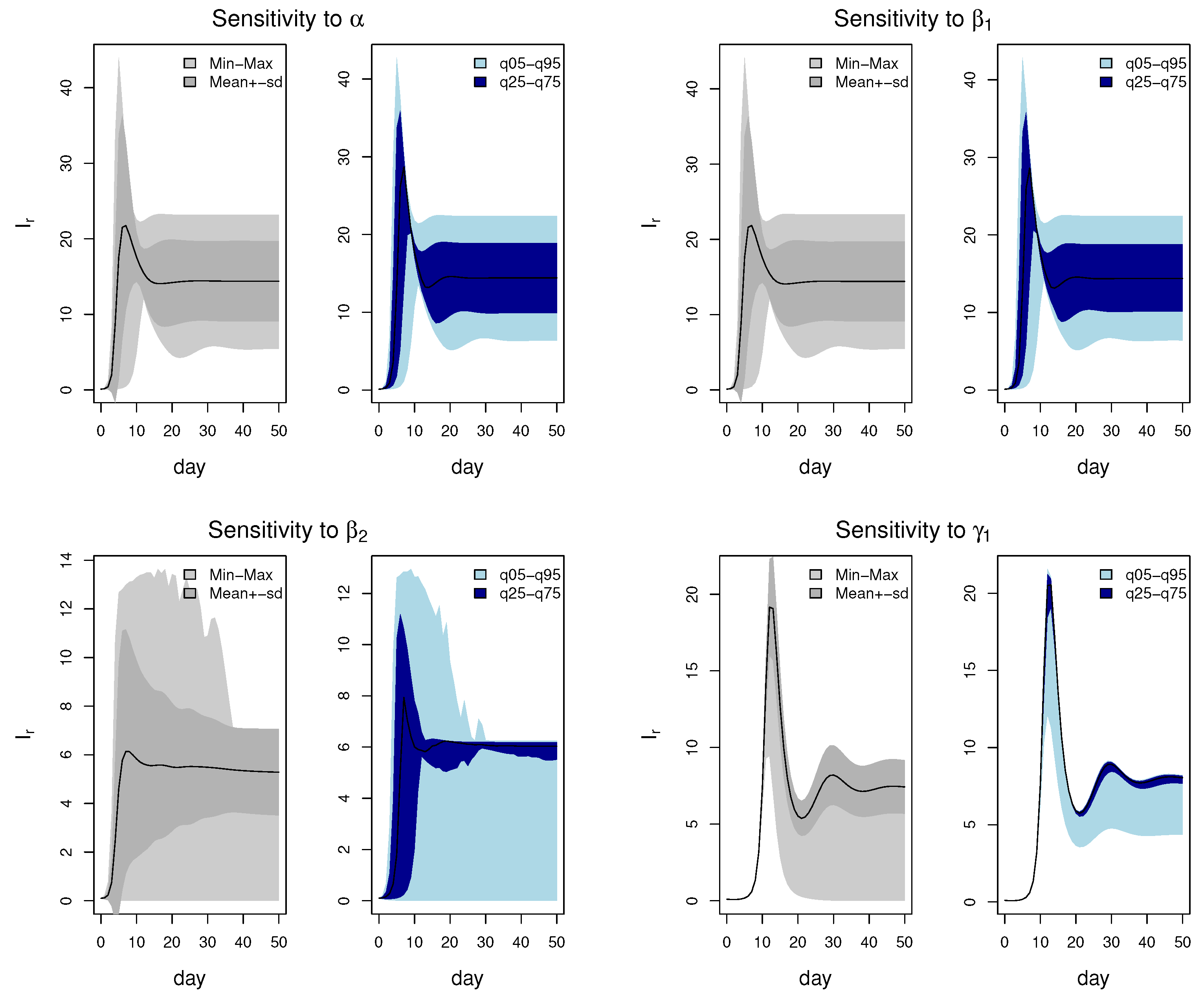
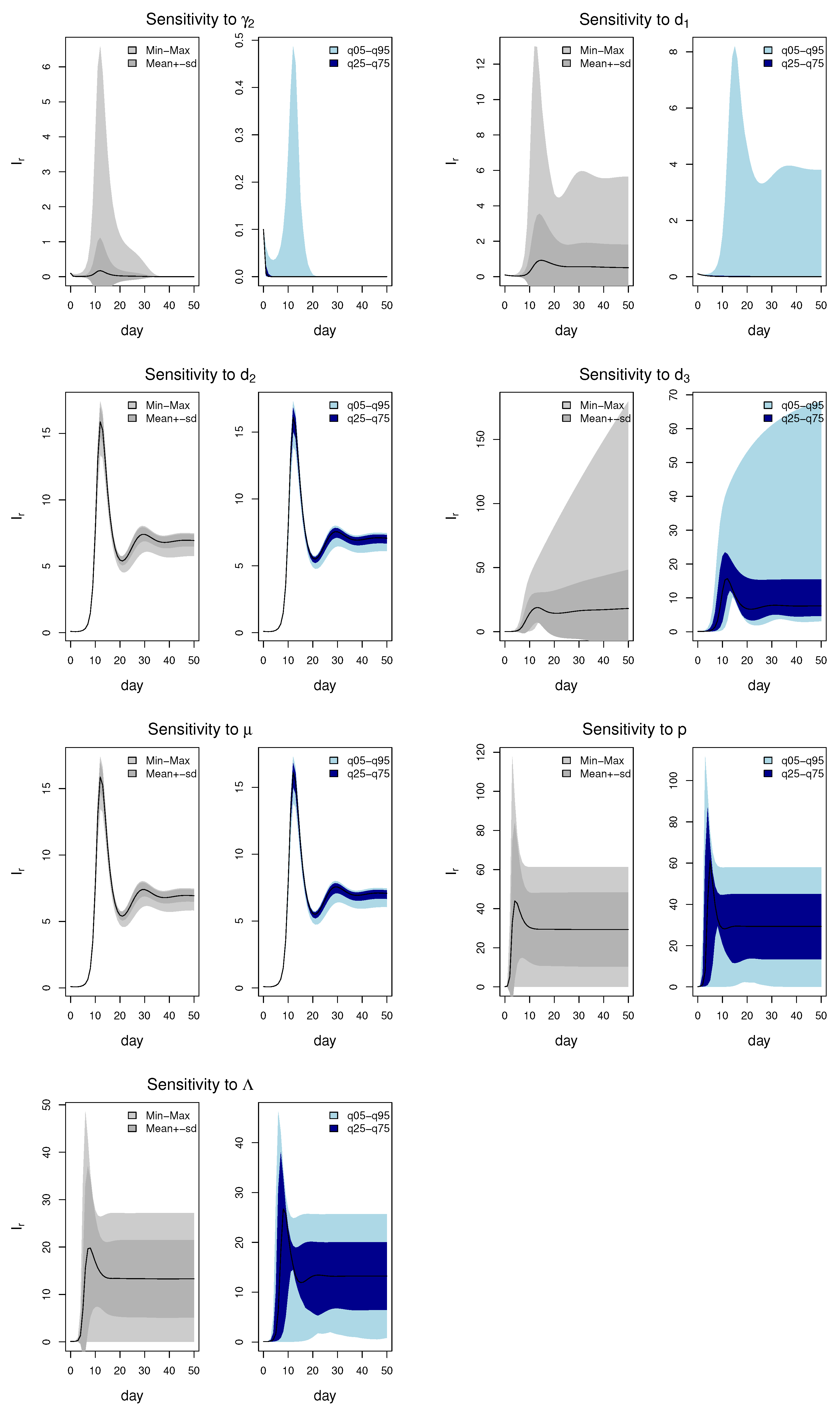
Local sensitivity refers to the sensitivity of parameters with respect to a given parameter set. This type of analysis is usually carried out by partial derivatives of the output functions at a fixed and predefined point of the parameter space. We are mainly concerned with the local sensitivity of the parameters we estimated in Table 1. The LSA results offered a sensitivity order, which is p, α , β 2 , Λ , d 3 , γ 1 , γ 2 , β 1 , d 1 , d 2 , μ from large to small by the measurement of L 1 and L 2 . The mean of the sensitivity index has the same direction as the equilibrium analysis results of each parameter. Table 3 and Figure 5 illustrate that d 2 and μ have a little effect on I r in the local parameter space, and p affect I r most near the estimated parameter, indicating that the proportion of drug-sensitive parasites released from an infected RBC by drug-resistance parasites is fairly important in a local parameter space. On the contrary, the direct effect of the decay rate of drug-sensitive parasites and the drug concentration was not significant may due to ignoring the interaction between these parameters.

3.4.2. Global Sensitivity Analysis

When the sensitivity index for an output variable is examined over the time course of the simulation, the relative importance of the parameters is shown to vary widely depending on the time point of inspection. The global sensitivity analysis results were obtained by employing the Sobol method, which provided a factor-based decomposition of the output variance. The first-order indices only account for the direct contribution of each parameter. The total Sobol indices quantified the fraction of the variance to explain the variability of each parameter full consideration of their interaction effects. Figure 6 depicts the first-order Sobol indices and the total Sobol indices; both of them range from 0 to 1 for all parameters. The first-order Sobol index of γ 2 is high in the first few days, but then decreases sharply, and other parameters remain zero in the concerned time course. The total Sobol index of γ 2 is high during the time interval, and p, Λ , β 2 , α , μ , and d 2 increase to a high value with time varying, indicating their relative importance to the drug-resistant strains. The other remaining parameters including β 1 , d 1 , and γ 1 are relatively less sensitive to resistant strains. Combining the two figures, we could deduce that, between those parameters, an interaction may exist.

4. Discussion and Conclusions

We have studied model (1) with the aim of exploring the impact of within-host competition and drug treatment on drug-resistant parasites. The results of our analysis have not only provided predictions, but have also painted a clearer picture of the influential parameters, laying the groundwork for the formulation of effective strategies in resistance management.
One of the key parameters, denoted as α , exhibits a significant correlation with drug-resistant parasites ( I r * ), underscoring the importance of the infected red blood cell’s capacity to produce merozoites. The infection process is characterized by repetitive cycles of invasions and merozoite production, as detailed by Anderson [34]. Consequently, inhibiting merozoite invasion of erythrocytes emerges as a viable strategy to reduce the number of drug-resistant parasites. The rate of malaria parasite infection plays a pivotal role in determining the invasive and infectious abilities of parasites [35]. As a result, variations in β 1 and β 2 can directly impact the population of drug-resistant parasites, as illustrated in Figure 3b,c. It is worth noting a phenomenon wherein increasing β 1 and β 2 leads to diminishing changes in I r * , suggesting that, within a certain range, adjusting the infection rate can effectively manage the evolution of drug resistance.
There is a growing interest in the potential of drug-based strategies beyond the initial treatment of malaria cases to further reduce morbidity and mortality and advance towards malaria elimination. Nevertheless, it is crucial to acknowledge the harsh reality that the emergence of resistance to anti-malarial drugs or combination therapies exposes the vulnerability of current strategies. The rapid elimination of drug-sensitive parasites can create a favorable environment for the survival of resistant parasites [24,36], a phenomenon well explained by the trends in I r * seen in Figure 3g,i. Furthermore, aggressive elimination of sensitive strains can lead to competitive release of drug-resistant parasites, given the absence of competitors (drug-sensitive parasites) to suppress them, highlighting the significance of competition between the two parasite types [16]. This relationship is depicted in Figure 3d,e, illustrating how the competitive ability of resistant strains directly affects their population. Another essential factor in the control of drug resistance is the genetic stability of resistant parasites, as evidenced by the decline in their numbers in Figure 3j. Hence, efforts to enhance the genetic stability of resistant parasites hold promise in resistance management. Finally, the tendencies of I r * in response to varying parameters such as Λ , d 1 , and d 3 are both reasonable and evident.
To further elucidate the sources of uncertainty, sensitivity analysis emerges as a fundamental technique, encompassing both local sensitivity analysis (LSA) and global sensitivity analysis (GSA). Typically, conducting LSA involves calculating the derivative of the outcome variable concerning each input parameter, making slight perturbations near the best point estimates. Numerous studies have delved into LSA, often by analyzing the basic reproduction number ( R 0 ) to examine disease equilibria in various epidemiological models [37,38]. In some cases, additional conditions are necessary because R 0 alone may not determine the existence of interior equilibria. Consequently, we have opted to directly focus on the interior equilibrium for our sensitivity analysis, utilizing numerical methods to gain deeper insights. Our LSA findings emphasize the significance of genetic instability and the number of merozoites in influencing the outcomes of the model. Intriguingly, drug concentration appears to be the least sensitive parameter to resistant strains. This observation may be attributed to the inherent limitations of LSA, which does not account for interactions between inputs, potentially making it challenging to establish a definitive ranking of the key parameters.
Global sensitivity analysis, on the other hand, excels in addressing this limitation by considering interactions among input parameters and varying all of them simultaneously within a certain range for epidemiological models. In contrast to LSA, GSA highlights the importance of μ , possibly due to its strong interactions with other parameters. Additionally, γ 2 maintains the highest sensitivity throughout the analysis, suggesting that drug therapy indirectly induces changes in the population of resistant parasites, potentially through competition dynamics. The implementation of aggressive treatment could trigger competitive release of drug-resistant parasites, as sensitive strains diminish. Hence, the competitive aspect should not be underestimated, and enhancing competition between the two strains may offer a viable approach to controlling drug-resistant parasites. The temporal variation in the sensitivity of state variables to parameters is a valuable aspect of infectious disease modeling studies [39]. Notably, the sensitivity of μ declines around the 40th day, possibly resulting from the elimination of drug-sensitive parasites by treatment, leaving fewer sensitive parasites to make a diminishing contribution. Parameters p, α , Λ , and β 2 continue to play a similarly crucial role compared to the LSA and maintain a high level of sensitivity throughout the simulation period.
Generally, Sobol global sensitivity analysis allows for accurate assessment of the parameters’ main effects and interactions and is applicable to various parameter space dimensions and model types, albeit with high computational costs. In contrast, MeFAST [40] incorporates the use of multiple statistical tests for the significance of the parameters; however, its performance may be suboptimal in highly nonlinear systems, and its evaluation of high-order interactions among parameters is limited. The Morris method [41] incurs lower computational costs, making it suitable for high-dimensional parameter spaces and complex models; nevertheless, its evaluation of interactions among parameters is limited. Derivative-based global sensitivity [40] assessment methods can provide rapid and accurate results, but are only applicable to differentiable functions and may have limited sensitivity evaluation capabilities for highly nonlinear systems. Therefore, when selecting methods, it is necessary to consider a combination of factors such as computational costs, applicability, and evaluation accuracy.
The model effectively aligns with the available data, yielding a set of estimated parameter values that form the foundation for subsequent analysis. In our investigation, we conducted equilibrium analysis, uncertainty analysis, and sensitivity analysis to explore the parameters that significantly influence and are chiefly responsible for the development of drug resistance. It is important to note that our study does not aim to directly propose specific drug resistance management strategies, but rather, intends to offer recommendations derived from mathematical findings and logical reasoning for more effective drug resistance control. The scope of this research solely considers the impact of drug treatment on sensitive strains. In future work, we plan to explore an extended dynamical system that incorporates the immune response into the model [42,43,44]. The immune response can play a pivotal role in preventing the re-invasion of merozoites or eliminating infected red blood cells [45].

Author Contributions

Conceptualization, T.S. and Y.W.; methodology, T.S.; software, Y.W.; validation, T.S., Y.W. and Y.L.; formal analysis, T.S.; writing—original draft preparation, T.S.; writing—review and editing, T.S.; visualization, Y.W.; supervision, G.F.; funding acquisition, Y.L. and G.F. All authors have read and agreed to the published version of the manuscript.

Funding

This research is partially supported by the National Natural Science Foundation of China (12101318, 12101393) and the National Social Science Foundation of China (22BTJ018).

Data Availability Statement

The data utilized in this study are derived from previously published works, which are openly available in [24] (https://www.pnas.org/doi/full/10.1073/pnas.1100299108, accessed on 11 May 2023). The specific datasets and their respective access details can be found within the referenced publications.

Acknowledgments

In the preparation of this paper, the author utilized Grammarly, an AI-assisted language editing tool, to enhance the grammatical correctness and fluency of our sentences.

Conflicts of Interest

The authors declare no conflict of interest.

References

  1. WHO. World Malaria Report 2020; WHO: Geneva, Switzerland, 2020. [Google Scholar]
  2. Nguyen, T.D.; Gao, B.; Amaratunga, C.; Dhorda, M.; Tran, T.N.A.; White, N.J.; Dondorp, A.M.; Boni, M.F.; Aguas, R. Preventing antimalarial drug resistance with triple artemisinin-based combination therapies. Nat. Commun. 2023, 14, 4568. [Google Scholar] [CrossRef] [PubMed]
  3. D’Alessandro, U.; Buttiëns, H. History and importance of antimalarial drug resistance. Trop. Med. Int. Health 2010, 6, 845–848. [Google Scholar] [CrossRef] [PubMed]
  4. WHO. Report on Antimalarial Drug Efficacy, Resistance and Response: 10 Years of Surveillance (2010–2019); WHO: Geneva, Switzerland, 2020. [Google Scholar]
  5. Dondorp, A.M.; Nosten, F.; Yi, P.; Das, D.; Phyo, A.P.; Tarning, J.; Lwin, K.M.; Ariey, F.; Hanpithakpong, W.; Lee, S.J.; et al. Artemisinin resistance in Plasmodium falciparum malaria. New Engl. J. Med. 2009, 361, 455–467. [Google Scholar] [CrossRef] [PubMed]
  6. Mathieu, L.C.; Cox, H.; Early, A.M.; Mok, S.; Lazrek, Y.; Paquet, J.C.; Ade, M.P.; Lucchi, N.W.; Grant, Q.; Udhayakumar, V.; et al. Local emergence in Amazonia of Plasmodium falciparum k13 C580Y mutants associated with in vitro artemisinin resistance. Elife 2020, 9, e51015. [Google Scholar] [CrossRef] [PubMed]
  7. Miotto, O.; Sekihara, M.; Tachibana, S.I.; Yamauchi, M.; Pearson, R.D.; Amato, R.; Gonçalves, S.; Mehra, S.; Noviyanti, R.; Marfurt, J.; et al. Emergence of artemisinin-resistant Plasmodium falciparum with kelch13 C580Y mutations on the island of New Guinea. PLoS Pathog. 2020, 16, e1009133. [Google Scholar] [CrossRef]
  8. Balikagala, B.; Fukuda, N.; Ikeda, M.; Katuro, O.T.; Tachibana, S.I.; Yamauchi, M.; Opio, W.; Emoto, S.; Anywar, D.A.; Kimura, E.; et al. Evidence of artemisinin-resistant malaria in Africa. New Engl. J. Med. 2021, 385, 1163–1171. [Google Scholar] [CrossRef] [PubMed]
  9. Acosta, M.M.; Bram, J.T.; Sim, D.; Read, A.F. Effect of drug dose and timing of treatment on the emergence of drug resistance in vivo in a malaria model. Evol. Med. Public Health 2020, 2020, 196–210. [Google Scholar] [CrossRef] [PubMed]
  10. Hastings, I. A model for the origins and spread of drug-resistant malaria. Parasitology 1997, 115, 133–141. [Google Scholar] [CrossRef]
  11. Mackinnon, M.J.; Hastings, I.M. The evolution of multiple drug resistance in malaria parasites. Trans. R. Soc. Trop. Med. Hyg. 1998, 92, 188–195. [Google Scholar] [CrossRef]
  12. Hastings, I.M.; D’Alessandro, U. Modelling a predictable disaster: The rise and spread of drug-resistant malaria. Parasitol. Today 2000, 16, 340–347. [Google Scholar] [CrossRef]
  13. Huijben, S.; Nelson, W.A.; Wargo, A.R.; Sim, D.G.; Drew, D.R.; Read, A.F. Chemotherapy, within-host ecology and the fitness of drug-resistant malaria parasite. Evolution 2010, 64, 2952–2968. [Google Scholar] [CrossRef] [PubMed]
  14. Wargo, A.R.; Huijben, S.; Roode, J.C.D.; Shepherd, J.; Read, A.F. Competitive release and facilitation of drug-resistant parasites after therapeutic chemotherapy in a rodent malaria model. Proc. Natl. Acad. Sci. USA 2007, 104, 19914–19919. [Google Scholar] [CrossRef]
  15. Bushman, M.; Morton, L.; Duah, N.; Quashie, N.; Abuaku, B.; Koram, K.A.; Dimbu, P.R.; Plucinski, M.; Gutman, J.; Lyaruu, P.; et al. Within-host competition and drug resistance in the human malaria parasite Plasmodium falciparum. Proc. Biol. Sci. 2016, 283, 20153038. [Google Scholar] [CrossRef]
  16. Hansen, E.; Woods, R.J.; Read, A.F. How to use a chemotherapeutic agent when resistance to it threatens the patient. PLoS Biol. 2017, 15, e2001110. [Google Scholar] [CrossRef]
  17. Whitlock, A.O.; Juliano, J.J.; Mideo, N. Immune selection suppresses the emergence of drug resistance in malaria parasites but facilitates its spread. PLoS Comput. Biol. 2021, 17, e1008577. [Google Scholar] [CrossRef]
  18. Ayala, M.J.; Villela, D.A. Early transmission of sensitive strain slows down emergence of drug resistance in Plasmodium vivax. PLoS Comput. Biol. 2020, 16, e1007945. [Google Scholar] [CrossRef] [PubMed]
  19. Mackinnon, M.J. Drug resistance models for malaria. Acta Trop. 2005, 94, 207–217. [Google Scholar] [CrossRef]
  20. Tchuenche, J.M.; Chiyaka, C.; Chan, D.; Matthews, A.; Mayer, G. A mathematical model for antimalarial drug resistance. Math. Med. Biol. 2011, 28, 335–355. [Google Scholar] [CrossRef] [PubMed]
  21. Hansen, J.; Day, T. Coinfection and the evolution of drug resistance. J. Evol. Biol. 2015, 27, 2595–2604. [Google Scholar] [CrossRef]
  22. Chiyaka, C.; Garira, W.; Dube, S. Effects of treatment and drug resistance on the transmission dynamics of malaria in endemic areas. Theor. Popul. Biol. 2009, 75, 14–29. [Google Scholar] [CrossRef]
  23. Fatmawati.; Tasman, H. An optimal control strategy to reduce the spread of malaria resistance. Math. Biosci. 2015, 262, 73–79. [Google Scholar] [CrossRef]
  24. Read, A.F.; Day, T.; Huijben, S. The evolution of drug resistance and the curious orthodoxy of aggressive chemotherapy. Proc. Natl. Acad. Sci. USA 2011, 108, 10871–10877. [Google Scholar] [CrossRef]
  25. Jurek, A.M.; Maldonado, G.; Greenland, S.; Church, T.R. Uncertainty analysis: An example of its application to estimating a survey proportion. J. Epidemiol. Community Health 2007, 61, 650–654. [Google Scholar] [CrossRef]
  26. Vesselinova, N.; Alexandrov, B.S.; Wall, M.E. Dynamical Model of Drug Accumulation in Bacteria: Sensitivity Analysis and Experimentally Testable Predictions. PLoS ONE 2016, 11, e0165899. [Google Scholar] [CrossRef] [PubMed]
  27. Song, T.; Wang, C.; Tian, B. Modelling intra-host competition between malaria parasites strains. Comput. Appl. Math. 2020, 39, 1–17. [Google Scholar] [CrossRef]
  28. Brauer, F.; Castillo Chavez, C. Mathematical Models in Population Biology and Epidemiology; Springer: Berlin/Heidelberg, Germany, 2001; pp. 267–291. [Google Scholar]
  29. Iman, R.L.; Helton, J.C. An investigation of uncertainty and sensitivity analysis techniques for computer models. Risk Anal. 2010, 8, 71–90. [Google Scholar] [CrossRef]
  30. Blower, S.M.; Dowlatabadi, H. Sensitivity and uncertainty analysis of complex models of disease transmission: An HIV model, as an example. Int. Stat. Rev. 1994, 62, 229–243. [Google Scholar] [CrossRef]
  31. Borgonovo, E. Sensitivity analysis of model output with input constraints: A generalized rationale for local methods. Risk Anal. 2010, 28, 667–680. [Google Scholar] [CrossRef] [PubMed]
  32. Sobol’, I.M. Sensitivity estimates for nonlinear mathematical models. Math. Model. Comput. Exp. 1993, 1, 407–414. [Google Scholar]
  33. Saltelli, A.; Annoni, P.; Azzini, I.; Campolongo, F.; Ratto, M.; Tarantola, S. Variance based sensitivity analysis of model output. Design and estimator for the total sensitivity index. Comput. Phys. Commun. 2010, 181, 259–270. [Google Scholar] [CrossRef]
  34. Anderson, R.M.; May, R.M.; Gupta, S. Non-linear phenomena in host-parasite interactions. Parasitology 1989, 99, S59–S79. [Google Scholar] [CrossRef]
  35. Hetzel, C.; Anderson, R.M. The within-host cellular dynamics of bloodstage malaria: Theoretical and experimental studies. Parasitology 1996, 113, 25–38. [Google Scholar] [CrossRef]
  36. Slater, H.C.; Okell, L.C.; Ghani, A.C. Mathematical modelling to guide drug development for malaria elimination. Trends Parasitol. 2017, 33, 175–184. [Google Scholar] [CrossRef]
  37. Samsuzzoha, M.; Singh, M.; Lucy, D. Uncertainty and sensitivity analysis of the basic reproduction number of a vaccinated epidemic model of influenza. Appl. Math. Model. 2013, 37, 903–915. [Google Scholar] [CrossRef]
  38. Dunn, J.M.; Davis, S.; Stacey, A.; Diuk-Wasser, M.A. A simple model for the establishment of tick-borne pathogens of Ixodes scapularis: A global sensitivity analysis of R 0. J. Theor. Biol. 2013, 335, 213–221. [Google Scholar] [CrossRef]
  39. Wu, J.; Dhingra, R.; Gambhir, M.; Remais, J.V. Sensitivity analysis of infectious disease models: Methods, advances and their application. J. R. Soc. Interface 2013, 10, 20121018. [Google Scholar] [CrossRef]
  40. Dela, A.; Shtylla, B.; de Pillis, L. Multi-method global sensitivity analysis of mathematical models. J. Theor. Biol. 2022, 546, 111159. [Google Scholar] [CrossRef]
  41. Qian, G.; Mahdi, A. Sensitivity analysis methods in the biomedical sciences. Math. Biosci. 2020, 323, 108306. [Google Scholar] [CrossRef]
  42. Chen, H.; Wang, W.; Fu, R.; Luo, J. Global analysis of a mathematical model on malaria with competitive strains and immune responses. Appl. Math. Comput. 2015, 259, 132–152. [Google Scholar] [CrossRef]
  43. Hellriegel, B. Modelling the immune response to malaria with ecological concepts: Short-term behaviour against long-term equilibrium. Proc. Biol. Sci. 1992, 250, 249–256. [Google Scholar]
  44. Li, Y.; Ruan, S.; Xiao, D. The within-host dynamics of malaria infection with immune response. Math. Biosci. Eng. 2013, 8, 999–1018. [Google Scholar]
  45. Stevenson, M.M.; Riley, E.M. Innate immunity to malaria. Nat. Rev. Immunol. 2004, 4, 169–180. [Google Scholar] [CrossRef] [PubMed]
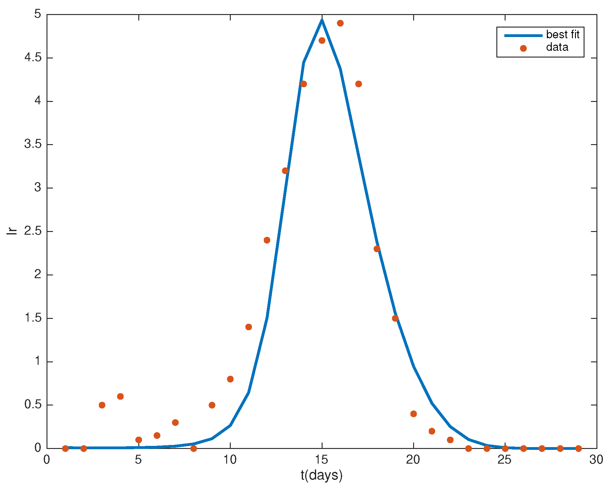
Figure 1. Drug-resistant parasites’ data (red dot) with model best fit (blue line). Each data point is assumed to have the same measurement error, estimated from competitive release of drug resistance data in the research of Read [24]. The y-axis is plotted using a log scale, reflecting the drug-resistant parasite density.
Mathematics 12 01595 g001
Figure 2. The solution curve of the model with the estimated parameters according to the data. The solid line, the dashed line, and the dotted line represent red blood cells, drug-sensitive parasites, and drug-resistant parasites, respectively.
Mathematics 12 01595 g002
Figure 3. Relationship between eleven sampled input parameters and equilibrium of I r . These results were obtained using a sample size of 1000. (a) I r vs. α . (b) I r vs. β 1 . (c) I r vs. β 2 . (d) I r vs. γ 1 . (e) I r vs. γ 2 . (f) I r vs. d 1 . (g) I r vs. d 2 . (h) I r vs. d 3 . (i) I r vs μ .
Mathematics 12 01595 g003
Figure 4. Uncertainty analysis of equilibrium of I r on all parameters.
Mathematics 12 01595 g004
Figure 5. Local sensitivity of state variable I r (drug-resistant parasites) on all parameters. The light grey region represents from the minimum value to the maximum value; the dark grey region is from the mean value minus the standard deviation to the mean value plus the standard deviation. The light blue region ranges from the 5th percentile to the 95th percentile; the dark blue region ranges from the 25th percentile to the 75th percentile.
Mathematics 12 01595 g005aMathematics 12 01595 g005b
Figure 6. Sobol sensitivity indices for state variable I r (drug-resistant parasites). The left graph depicts the tendency of the first-order Sobol index, and the right graph describes the total sobol index of all model parameters.
Mathematics 12 01595 g006
Table 1. Parameters in the model.
ParameterDefinitionEstimated ValueRangeRef.
α number of merozoites that an infected RBC can produce8.559469[8, 32]
β 1 infection rate of drug-sensitive malaria parasites 1.497515 × 10 4 [0, 1]
β 2 infection rate of drug-resistant malaria parasites0.03018763[0, 1]
γ 1 competitive coefficient0.08115581[0, 1]
γ 2 competitive coefficient0.003323166[0, 1]
Λ production rate of RBCslog10 (41,500) [34]
d 1 decay rate of RBCs0.00833 [34]
d 2 decay rate of drug-sensitive malaria parasites 1.497515 × 10 4 [0, 1]
d 3 decay rate of drug-resistant malaria parasites0.6355716[0, 1]
μ level of drug concentration 1.497515 × 10 4 [0, 1]
pproportion of drug-sensitive parasites released0.8605191[0, 1]
from an infected RBC by drug-resistance parasites
Table 2. Descriptive statistics from the uncertain analysis of Ir in Figure 4.
MinimumMaximumMeanMedianVariance5th Percentile5th Percentile
4.610 ×   10 5 200.314216.586810.7515398.99291.521951.7296
Table 3. Value of local sensitivity function.
Para α β 1 β 2 γ 1 γ 2 Λ d 1 d 2 d 3 μ p
L 1   a 7.70.465.62.72.46.70.30.000826.60.0008262
L 2   a 1.60.00761.50.440.41.30.00620.000131.10.0001312
M e a n   b 6.4−0.461.32.7−2.46.2−0.280.00082−6.60.00082−60
a Here, L 1 = | S i | / n , L 2 = ( S i 2 ) / n are the L 1 - and L 2 -norm, respectively. b The Mean column is the mean of the sensitivity functions.
Disclaimer/Publisher’s Note: The statements, opinions and data contained in all publications are solely those of the individual author(s) and contributor(s) and not of MDPI and/or the editor(s). MDPI and/or the editor(s) disclaim responsibility for any injury to people or property resulting from any ideas, methods, instructions or products referred to in the content.