Abstract
In order to enhance the trajectory tracking accuracy of distributed-driven intelligent vehicles, this paper formulates the tasks of torque output control for longitudinal dynamics and steering angle output control for lateral dynamics as Markov decision processes. To dissect the requirements of action output continuity for longitudinal and lateral control, this paper adopts the deep deterministic policy gradient algorithm (DDPG) for longitudinal velocity control and the deep Q-network algorithm (DQN) for lateral motion control. Multi-agent reinforcement learning methods are applied to the task of trajectory tracking in distributed-driven vehicle autonomous driving. By contrasting with two classical trajectory tracking control methods, the proposed approach in this paper is validated to exhibit superior trajectory tracking performance, ensuring that both longitudinal velocity deviation and lateral position deviation of the vehicle remain at lower levels. Compared with classical control methods, the maximum lateral position deviation is improved by up to 90.5% and the maximum longitudinal velocity deviation is improved by up to 97%. Furthermore, it demonstrates excellent generalization and high computational efficiency, and the running time can be reduced by up to 93.7%.
Keywords:
distributed drive autonomous vehicles; trajectory tracking; multi-agent deep reinforcement learning; deep deterministic policy gradient; deep Q-network MSC:
68T42
1. Introduction
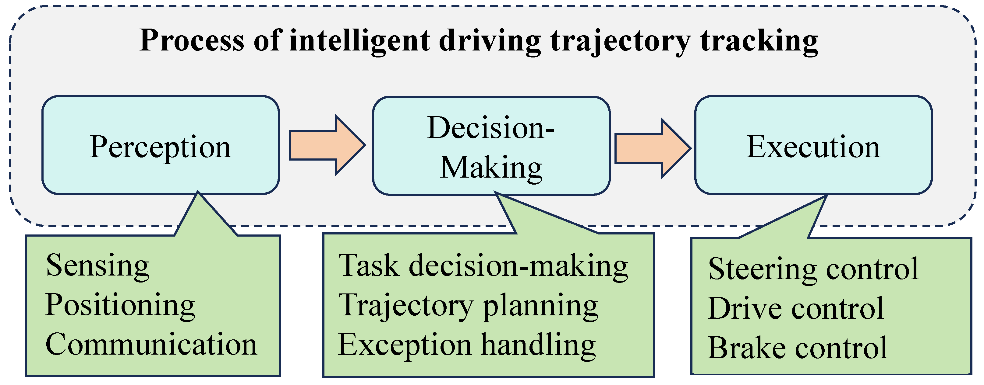
In recent years, distributed drive autonomous vehicles (DDAVs), integrating distributed electric propulsion, have emerged as a pivotal direction in automotive technological advancement because of their notable advantages in energy efficiency, environmental friendliness, rapid response, simple structure, and high transmission efficiency [1,2]. As illustrated in Figure 1, the realization of intelligent vehicle trajectory tracking involves three main stages including perception, decision-making, and execution. Execution (motion control) represents the final frontier in intelligent driving, with trajectory tracking standing at its core. This involves orchestrating the longitudinal and lateral motion control of vehicles through the control of chassis systems such as drive, braking, and steering, enabling precise tracking of desired longitudinal velocities and timely arrival at corresponding reference trajectory points [3]. It is evident from this analysis that the execution phase, encompassing longitudinal and lateral vehicle motion control, constitutes a pivotal determinant of the precision in vehicle trajectory tracking. Simultaneously, the speed of computations plays a crucial role in determining the efficacy of control, particularly in hazardous scenarios. The enhancement of computational speed in the execution phase is therefore vital for improving safety measures. Hence, augmenting both the precision of control and computational speed within the trajectory tracking execution phase emerges as imperative for the advancement of intelligent vehicle driving technology.

Figure 1.
Process of intelligent driving trajectory tracking.
In the current academic discourse on trajectory tracking for intelligent vehicles, the mainstream approach involves separately designing lateral motion controllers and longitudinal motion controllers, which are then combined. However, these designed control laws often demand high precision in vehicle dynamic parameters and computational resources [4,5,6,7,8,9]. Common methods for designing longitudinal controllers include proportional–integral–derivative (PID) methods, sliding mode control algorithms, or model predictive control (MPC) methods. These methods achieve autonomous driving longitudinal speed tracking by directly outputting vehicle acceleration or braking torque. Some scholars have proposed improvements to these methods; for instance, reference [10] combines PID methods with radial basis function neural networks to enhance robustness. Reference [11] presents an adaptive sliding mode control method, introducing parameter adaptation laws to compensate for variations in environmental disturbances and model uncertainties. Reference [12] employs MPC algorithms to design hierarchical controllers for distributed-driven vehicles, achieving autonomous driving longitudinal speed tracking and verifying control performance. Reference [13] combines neural networks with sliding mode control algorithms, resulting in an improved adaptive sliding mode control algorithm with better robustness. As for lateral controllers, they aim to stabilize the tracking of desired trajectories by controlling vehicle steering. Currently, they can be categorized into two types as follows: those based on kinematic control and those based on dynamic control. The design of specific control laws mostly involves PID methods, pure tracking algorithms, Linear Quadratic Regulator (LQR) methods, and MPC-based methods. Scholars have also made corresponding improvements in this domain. For example, reference [14] enhances PID methods based on kinematic models, which exhibit improved robustness with the introduction of neural networks. Reference [15] proposes an adaptive pure tracking algorithm based on kinematic models, effectively reducing tracking errors by combining PI control with pure tracking algorithms. Reference [16] proposes an online adaptive module for tire parameters in MPC controllers based on vehicle dynamic models, updating parameters online to reduce model mismatch and enhance the robustness of lateral motion controllers.
However, the dynamic response of DDAV exhibits not only strong nonlinearity but also uncertainty and time-varying characteristics, which can affect the precision of the aforementioned control laws. Compared with mainstream methods, the integration of neural networks can effectively enhance control effectiveness and robustness [17,18,19]. Therefore, some scholars propose utilizing deep reinforcement learning (DRL), which requires less computational power and lower precision of mathematical models in handling nonlinear control problems. Deep reinforcement learning (DRL) is an amalgamation of deep learning and reinforcement learning, possessing both the feature extraction capabilities of deep neural networks and the decision-making advantages of reinforcement learning. It enables end-to-end learning, from perception to decision control, based on deep neural networks. DRL methods engage in trial-and-error learning through interaction with the environment, allowing the model to explore and obtain optimal decision-making for control systems autonomously. Common algorithms such as DQN, DDPG, and DDQN exemplify DRL’s versatility. DRL finds extensive applications in fields like communication control, mechanical control systems, autonomous driving, and intrusion detection systems (IDSs) [20]. Reference [21] applied DRL to traffic control without lanes, designing reward and penalty functions to maintain vehicle ideal speeds while minimizing collisions among vehicles. Reference [22] developed a vision-based DRL autonomous driving agent, which, utilizing patterns detected by perception modules on lane markings and the rear end of preceding vehicles, achieved lane-keeping and car-following tasks. Reference [23] employed DRL to train agents capable of autonomously overtaking both stationary and moving vehicles on roads while avoiding collisions with obstacles ahead and to the right. Reference [24] utilized DRL in conjunction with hybrid A* path planning for parking maneuvers in autonomous vehicles, addressing the issue of traditional model predictive control (MPC) methods’ lack of consideration for the right-of-way of traffic participants in trajectory planning. References [25,26] employ reinforcement learning methods to design autonomous driving longitudinal controllers, achieving vehicle speed cruising by directly controlling vehicle acceleration for autonomous braking and driving. References [27,28] apply reinforcement learning methods to design steering control strategies, enabling trained agents to perform lane changes or turning actions by outputting front wheel angles in autonomous driving environments. It is evident that applying DRL to trajectory tracking control for intelligent vehicles and using single-agent DRL methods in the design of individual longitudinal or lateral controllers demonstrate unique advantages. However, most of these approaches combine mainstream control methods with DRL methods, failing to exploit the advantages of DRL fully.
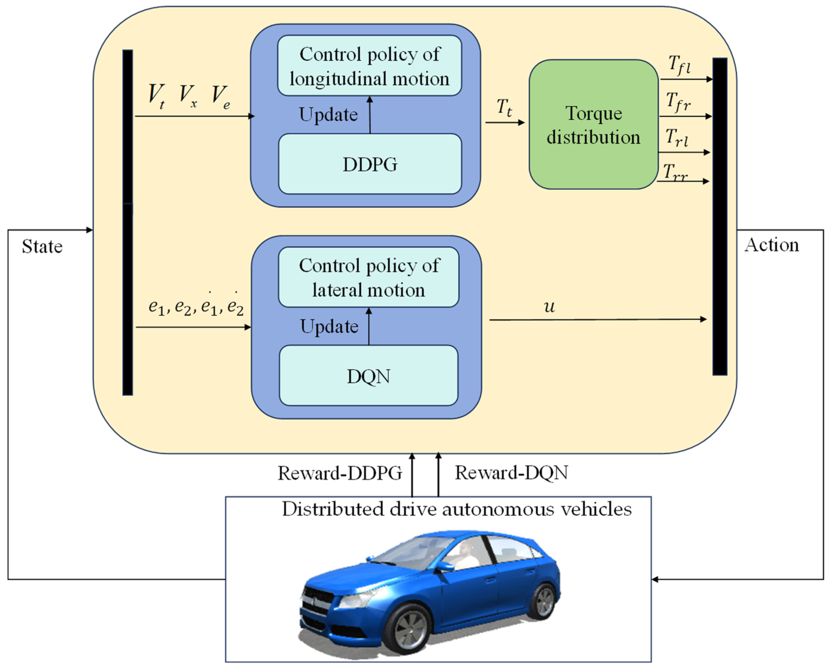
To address this, our study applies multi-agent systems to the trajectory tracking task of distributed-driven vehicles with distributed drive characteristics. Based on this idea, we propose a distributed drive autonomous vehicle (DDAV) trajectory tracking control method based on multi-agent deep reinforcement learning (MADRL), as illustrated in Figure 2. The main contributions are listed as follows:
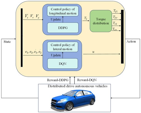
Figure 2.
The structure of the control system.
(1) Employing MADRL for trajectory tracking controller design, utilizing distributed training among agents, and continuously training and iterating using deep reinforcement learning methods by designing reward and penalty functions and corresponding networks. This approach aims to achieve optimal longitudinal and lateral control while approaching the global optimum to the maximum extent, thereby improving upon mainstream control methods that require high precision in parameters and are prone to “local optima” issues, with higher operational efficiency.
(2) Moreover, to fully exploit the traction capabilities of each driving wheel in distributed-driven vehicles, an optimization approach is employed to design the longitudinal torque distribution controller at the lower level, optimizing the distribution of torque commands executed by each drive motor.
(3) Through simulation, it is verified that the proposed distributed drive autonomous vehicle trajectory tracking control based on the multi-agent deep reinforcement learning method has good trajectory tracking performance and high computational efficiency under different working conditions and different speeds.
2. Trajectory Tracking Control for DDAVs Based on MADRL
Deep reinforcement learning can be understood as the integration of deep learning and reinforcement learning. Deep learning is responsible for function approximation using deep neural networks, while reinforcement learning represents the iterative training process. Within this framework, agents are defined within the system. These agents interact with the environment and states, taking actions based on predetermined reward or penalty functions. Through continuous training, the goal is to maximize the total reward, updating the control policies within the agents.
2.1. Analysis of Longitudinal and Lateral Motion Control for DDAVs
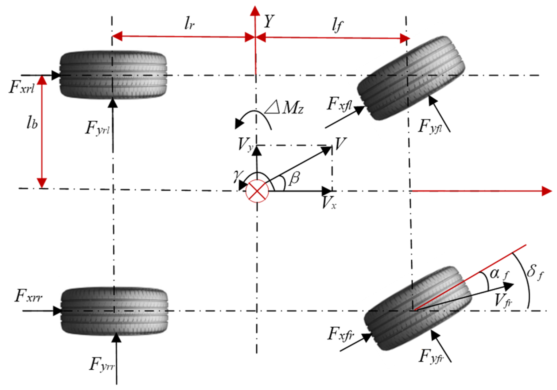
In this section, the mathematical formulation of the dynamic control theory for DDAVs is presented. Firstly, the three-degree-of-freedom model of DDAVs is described, as shown in Figure 3. In the realm of vehicle dynamics, commonly employed models include the two-degree-of-freedom vehicle model, the three-degree-of-freedom vehicle model, and the seven-degree-of-freedom vehicle model, which can capture distributed drive characteristics. The two-degree-of-freedom vehicle model simplifies vehicle dynamics by disregarding suspension effects, treating the vehicle as a two-wheeled entity, assuming linear tire lateral characteristics, and neglecting longitudinal driving or resistance forces, thereby considering longitudinal velocity as constant and only representing vehicle yaw and lateral motion. The three-degree-of-freedom vehicle model builds upon the two-degree-of-freedom model by introducing an additional degree of freedom for longitudinal motion while keeping the other two degrees of freedom unchanged for lateral motion and yaw motion. Building upon the foundation of the three-degree-of-freedom model, it is extended to a seven-degree-of-freedom model, which accounts for both lateral, longitudinal, and yaw motions of the vehicle, as well as the rotational states of all four wheels. This extended model comprehensively captures the driving characteristics of the entire vehicle while reflecting the distributed drive nature of DDAVs [29].
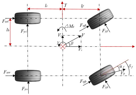
Figure 3.
Three-degree-of-freedom model for DDAVs.
In the above equations, represents the total vehicle mass; is the longitudinal force of the tire; is tire lateral force (i represents the front wheel or rear wheel, and j represents the left wheel or right wheel); denotes the longitudinal velocity of the vehicle; represents the lateral velocity; is the yaw rate of the vehicle; is the yaw inertia coefficient of the vehicle; is the average front wheel steering angle; is the sideslip angle; and are the distances from the center of gravity to the front and rear axles, respectively; is half of the wheelbase; and is the forward speed of the vehicle.
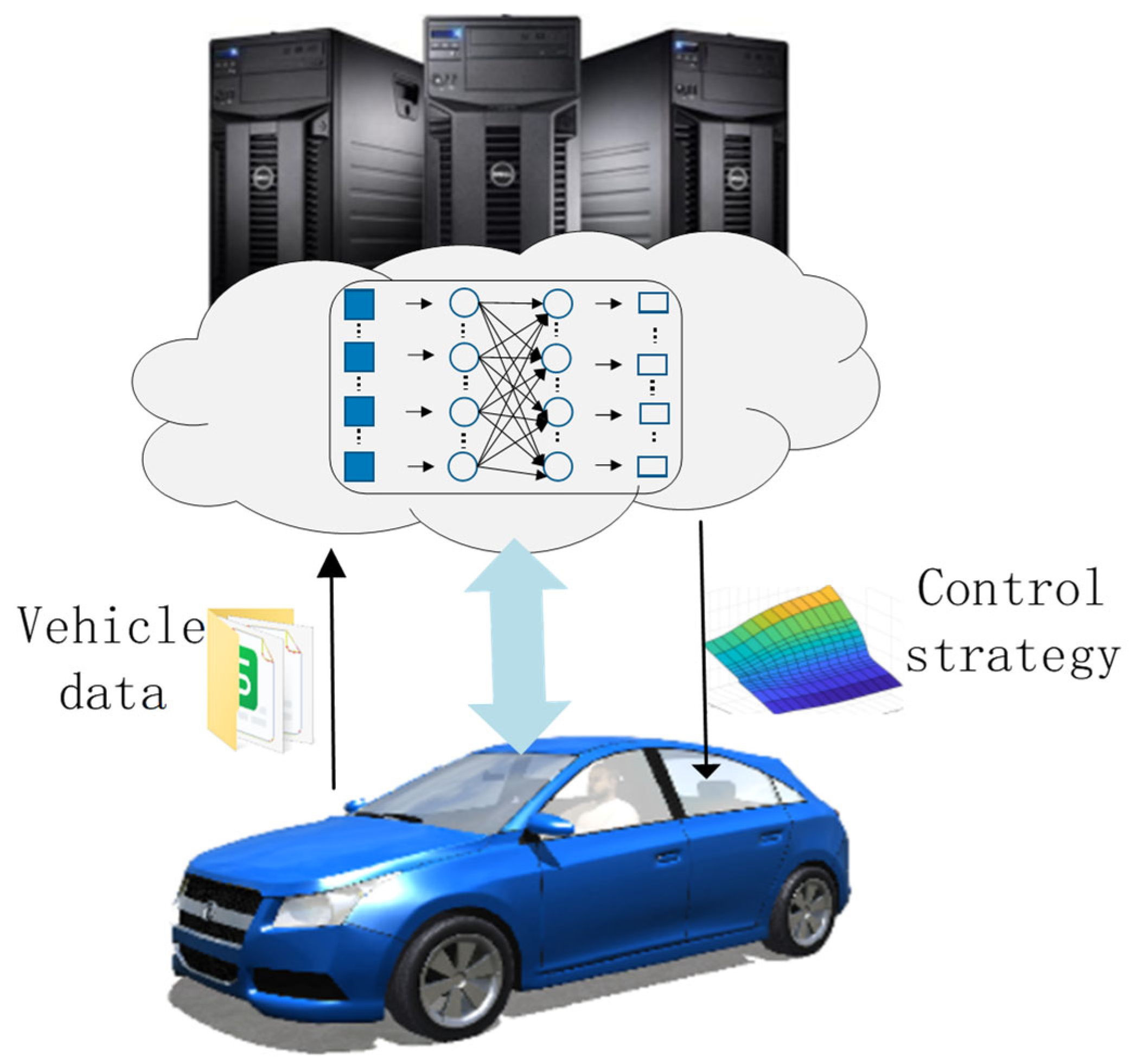
In the current scholarly discourse surrounding longitudinal and lateral motion control in autonomous driving vehicles, the predominant methodology largely entails the establishment of a two-degree-of-freedom reference model. This model serves as the basis for deriving control objectives such as the desired yaw rate and lateral deviation angle of the center of mass. Subsequently, a simplified linearization of the tire model is applied to facilitate kinematic control. However, within the context of the seven-degree-of-freedom model of DDAVs, it becomes evident that joint longitudinal and lateral motion control in real vehicle systems is subject to three primary coupling effects including kinematic coupling, load transfer coupling, and tire force coupling [30]. Notably, the dynamic response of both vehicles and tires manifests significant nonlinearity, alongside uncertainties and time-varying characteristics. These factors pose challenges to the precision of mainstream control methods. Moreover, errors in parameter estimation can profoundly impact the adaptability of control laws across various operational conditions. Consequently, the machine learning algorithms introduced in this study offer a comprehensive solution to address the shortcomings of mainstream control methods in terms of precision, efficiency, and robustness. Furthermore, as illustrated in Figure 4, the practical implementation of deep reinforcement learning methods during vehicle operation enables continuous training throughout the vehicle’s lifecycle and periodic policy iteration. This approach significantly reduces the reliance on high-precision mathematical models of vehicles and computational resources when compared with mainstream control methods.
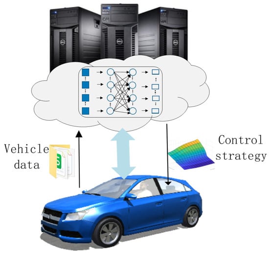
Figure 4.
Training and iteration throughout the DDAV lifecycle.
2.2. Design of the MADRL Controller
As stated earlier, trajectory tracking in DDAVs is a responsive outcome under multi-execution system control involving both the propulsion and steering systems. Because of the transformation between the vehicle’s coordinate system and the global coordinate system, the steering system not only induces lateral position changes but also affects the vehicle’s longitudinal velocity [31]. Therefore, when employing deep reinforcement learning methods for joint longitudinal and lateral control of DDAVs, the complexity arises from the multitude of vehicle state indicators and control objectives. Simple control design with a single agent may lead to difficulties in setting reward functions and coordinating priority relationships. Unlike single-agent deep reinforcement learning, MADRL partitions the action space into different subspaces and assigns them to different agents. This effectively reduces the complexity of network design for each agent, allowing multiple control strategies to be trained independently by different agents [32]. Consequently, this approach enables the independent setting of states, actions, and rewards for more targeted training.
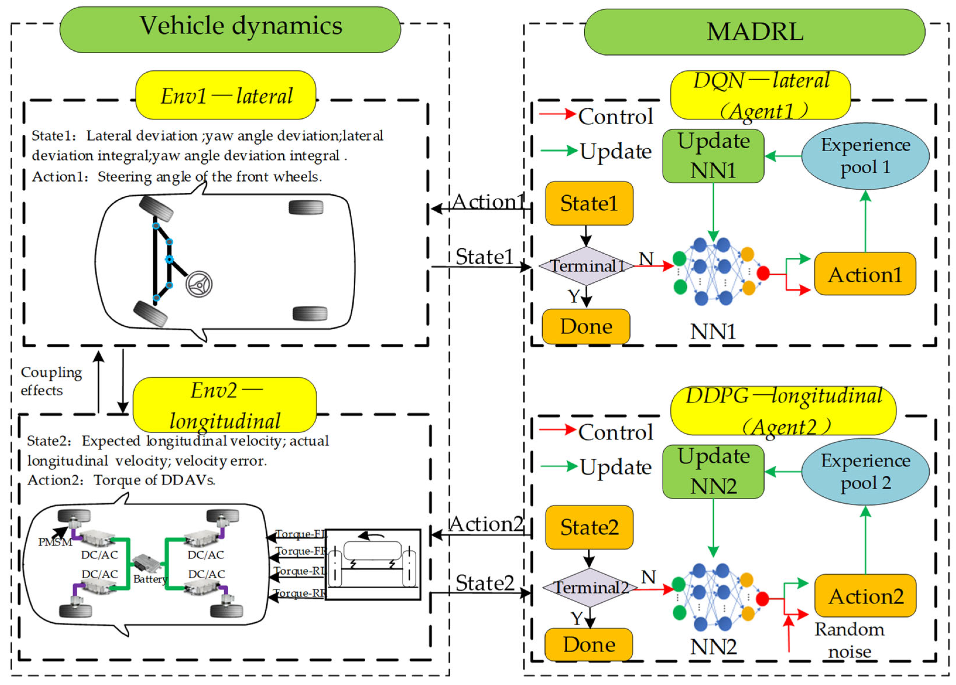
The trajectory tracking control strategy proposed in this paper, as illustrated in Figure 5, consists of the DDAV system, lateral control Agent1, and longitudinal control Agent2. Upon receiving the vehicle state, Agent1 outputs steering commands applied to the front wheels while updating its own neural network. Agent2 outputs torque commands and utilizes a lower-level allocator to output motor longitudinal torque to drive the vehicle to track the desired longitudinal velocity, simultaneously updating its own neural network. In DDAVs, the driving motor executes torque actions, and the steering actuator executes steering actions, which, based on kinematic coupling, load transfer coupling, and tire force coupling relationships, induce changes in the overall vehicle state. Corresponding reward values are generated based on reward functions for each agent to train and update according to set parameters.
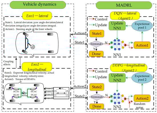
Figure 5.
Diagram of the proposed DDAV trajectory tracking based on MADRL.
2.2.1. Design of Reward or Penalty Functions
The Markov Decision Process (MDP) refers to a system where the current state depends only on the preceding state and action. In the trajectory tracking process of DDAVs, each agent’s action leads to an update in the DDAV to a new state. Based on the DDAV’s state, corresponding rewards are generated. Through iterative training, the neural networks of the agents achieve effective training. Therefore, the longitudinal and lateral control processes of DDAVs can be regarded as MDPs.
In the above equation, represents the initial state, denotes the state value, represents the action value, corresponds to the reward, is the total time duration, and is the action space.
The future cumulative reward obtained after executing action in state according to the control strategy can be defined as . is used to evaluate action .
In the above equation, denotes discount factor, .
If the optimal action is chosen in a certain state , then the corresponding optimal is obtained at that moment.
The optimal control policy can be represented as follows:
To achieve the DDAV trajectory tracking objective, the state variables, action variables, and reward–penalty functions for the lateral and longitudinal controllers are defined as follows:
- (1)
- Agent for lateral control
The control problem of the lateral control agent is described as shown in Equation (8), where is the set of observed values generated by the environment, defined as the lateral position deviation in the vehicle, the yaw angle deviation of the vehicle, and their respective rates of change and . is the set of action spaces, defined as the front wheel steering command . is the reward and punishment function evaluating the performance of the steering controller. To ensure the accuracy of trajectory tracking while minimizing the output of unnecessary steering actions, the reward and punishment function consists of position deviation and its rate of change, yaw angle deviation and its rate of change, and front wheel steering action; is the weight coefficient. In this paper, for the convenience of training the agent, it is necessary to normalize each component of the reward and punishment function before input.
In the above equation, the inclusion of is motivated by the aim to minimize steering interventions while fulfilling trajectory tracking requirements, thereby enhancing the driving experience. This approach prioritizes reducing steering maneuvers without excessively pursuing tracking precision, which could otherwise lead to continual fine adjustments of steering angles. The adjustment process of the weights is a human-driven endeavor, necessitating iterative cycles of experimentation, training, observation, and refinement.
In the above equation, represents the lateral position deviation of the vehicle and represents the yaw angle deviation of the vehicle:
In the above equation, represents the expected lateral position of the vehicle at the given moment; denotes the actual lateral position of the vehicle at that moment; signifies the expected yaw angle of the vehicle at the given moment; and represents the actual yaw angle of the vehicle at that moment.
The action space constraint is defined as:
In the above equation, and correspond, respectively, to the actual range of the front wheel steering angles of the vehicle.
However, because of the strong generality of DRL, there is significant randomness in action selection during the early stages of training, leading to extensive useless exploration and resulting in inefficiencies in exploration, lengthy training cycles, and poor training outcomes. Combining rule-based control strategies is an effective means of efficiently utilizing reinforcement learning tools. When states match predefined rules, priority is given to these rules; otherwise, reinforcement learning is employed for exploration. In this paper, a rule-based terminal state design for the agent is proposed. Terminal states typically correspond to the conclusion of a training episode, often defined by the number of steps to trigger episode termination. Building upon a step-based terminal state framework, this study introduces a rule-based terminal state design. When the current state matches predefined rules for terminating an episode prematurely, the training cycle with unsatisfactory performance can be ended prematurely, allowing for the commencement of the next training cycle to reduce futile exploration in the current cycle.
The terminal conditions for lateral control agent are defined as follows:
- (2)
- Agent for longitudinal control
The control problem of the longitudinal control agent is described as shown in Equation (12), where represents the set of observed values generated by the environment, specifically, the desired longitudinal velocity of the vehicle, the actual longitudinal velocity , and their deviation . denotes the action space set, representing the longitudinal force torque exerted by the drive motor . is the reward and punishment function evaluating the performance of the longitudinal velocity controller. To ensure precision in maintaining longitudinal velocity while minimizing abrupt accelerations or decelerations, the reward and punishment function comprises longitudinal velocity deviation and vehicle acceleration, as well as an individual reward component and an individual punishment component . The introduction of individual reward and punishment components aims to provide substantial rewards for minimal velocity deviations or impose significant penalties for substantial velocity deviations, thus better guiding the training process. represents the weight coefficient. In this paper, for the convenience of training the agent, it is necessary to normalize the inputs of and within the reward and punishment function before processing.
In the above equation, longitudinal velocity deviation can be defined as:
the individual reward component can be defined as:
and the individual punishment component can be defined as:
The terminal conditions for the longitudinal control agent are defined as follows:
It should be noted that the adjustment of the weights / in Equations (8) and (12) is an artificial process, which requires continuous trial, training, observation, and adjustment until the desired training effect is achieved.
To fully exploit the adhesion capability of the driving wheels, a longitudinal torque distribution controller is designed at the lower level of the longitudinal control intelligent agent to optimize the allocation of torque commands sent to each driving motor. When the vehicle is traveling straight, the vertical loads on both sides of the driving wheels are equal. However, during steering, the vehicle’s center of gravity shifts outward because of centrifugal force, resulting in an increase in the vertical load on the outer wheel and a decrease in the load on the inner wheel [33]. The concept of “friction ellipse” can be used to express the road adhesion load of a single wheel:
In the above equation, represents the longitudinal force of the driving wheel, represents the lateral force of the driving wheel, represents the vertical load on the driving wheel, and represents the road adhesion coefficient.
If we assign weight coefficients to each wheel, denoted as , the function for the overall vehicle’s road adhesion load can be expressed as follows:
The smaller the function for the overall vehicle’s road adhesion load, the greater the adhesion margin. As it is not feasible to actively control the lateral forces exerted on the wheels, the objective function for optimization allocation is:
In the above equation, represents the torque commands sent to each driving motor and represents the rolling radius of the driving wheel.
Additionally, the constraint boundaries for the optimization allocation controller are:
2.2.2. Design of DQN and DDPG Networks
In the process of autonomous driving, commands for the line-controlled steering motor can be discretely outputted. Discrete command output typically entails simpler control logic, ensuring real-time capability and implementation simplicity of the line-controlled steering motor controller, while also meeting the requirements of the steering system. Moreover, because of the fixed values and ranges of discrete commands, it becomes easier to predict and control the vehicle’s steering behavior, thereby enhancing system stability and controllability. However, the adjustment requirements for the vehicle’s power output section are more refined. Discrete command output may affect the driving comfort of the vehicle. Considering that in operational scenarios of the vehicle, there is a greater emphasis on controlling longitudinal speed, and aiming to fully leverage the advantages of deep reinforcement learning algorithms such as DQN and DDPG in different control dimensions [34], enhancing system robustness and flexibility while reducing the complexity of algorithm design, the DQN algorithm is adopted for lateral control Agent1, while the DDPG algorithm is employed for longitudinal speed control Agent2.
Q-learning aims to maximize by selecting the optimal action for each state and updating it accordingly.
In the above equation, represents the current state, denotes the current action, signifies the next moment’s state, represents the action at the next moment, is the learning rate, denotes the reward, and is the decay coefficient.
In the DQN algorithm employed by the lateral control agent, the training samples for deep learning are derived from reinforcement learning data. The neural network in deep learning performs computations on input data through operations such as convolution, pooling, and fully connected layers, generating action Q-values. Subsequently, the loss function is computed based on the difference between these Q-values and the correct Q-values provided by reinforcement learning. The deep learning network’s weights are then adjusted according to the loss function.
Therefore, the loss function for DQN is
In the above equation, represents the neural network parameters.
Upon obtaining the loss function, DQN utilizes stochastic gradient descent to compute gradients, aiming to minimize the loss and drive action values toward maximization.
Additionally, because of the inherent Markovian property of reinforcement learning, which results in high correlation among training samples—an aspect inconsistent with the requirements of deep learning—DQN incorporates an experience replay mechanism, as illustrated in Equation (24):
Storing samples in a sample pool is employed to calculate the gradient of the loss function and update the neural network parameters, ensuring independence among samples.
DQN also introduces a target network, which calculates temporal difference errors when solving the loss function.
Exclusively utilizing the online network to obtain and would result in synchronous variations, leading to non-convergence of the loss function. Therefore, calculations are performed separately using both the online network and the target network. The target network directly copies the real-time parameters of the online network to update its parameters after a certain number of time steps.
Simultaneously, to avoid falling into local optima, DQN employs an ε-greedy strategy when selecting actions. Specifically, with a probability of , it selects the action with the maximum Q value, and with a probability of , it chooses a random action.
The DDPG algorithm employed by the longitudinal control agent consists of two networks as follows: the actor and the critic. Each network includes both a current network and a target network, denoted by and , representing the parameters for the actor and critic networks, respectively. In the actor network, is updated based on the value function, and actions are generated according to the current state. The critic network updates using the network gradient and evaluates the value of actions. The critic network updates its network parameters by minimizing the loss function, which is expressed as follows:
In the above equation, denotes discount factor.
The actor network updates its network parameters using deterministic policy gradients:
Simultaneously, the parameters of the two target networks in DDPG are updated using a “soft update” approach, which effectively prevents oscillation and divergence:
In the above equation, denotes the target smooth factor.
DDPG also incorporates the experience replay mechanism from DQN.
By sampling from the environment and placing the samples into a pool, random mini-batches of data are extracted for learning updates. The execution of actions is obtained as follows:
In the above equation, represents random noise and denotes the optimal behavioral policy.
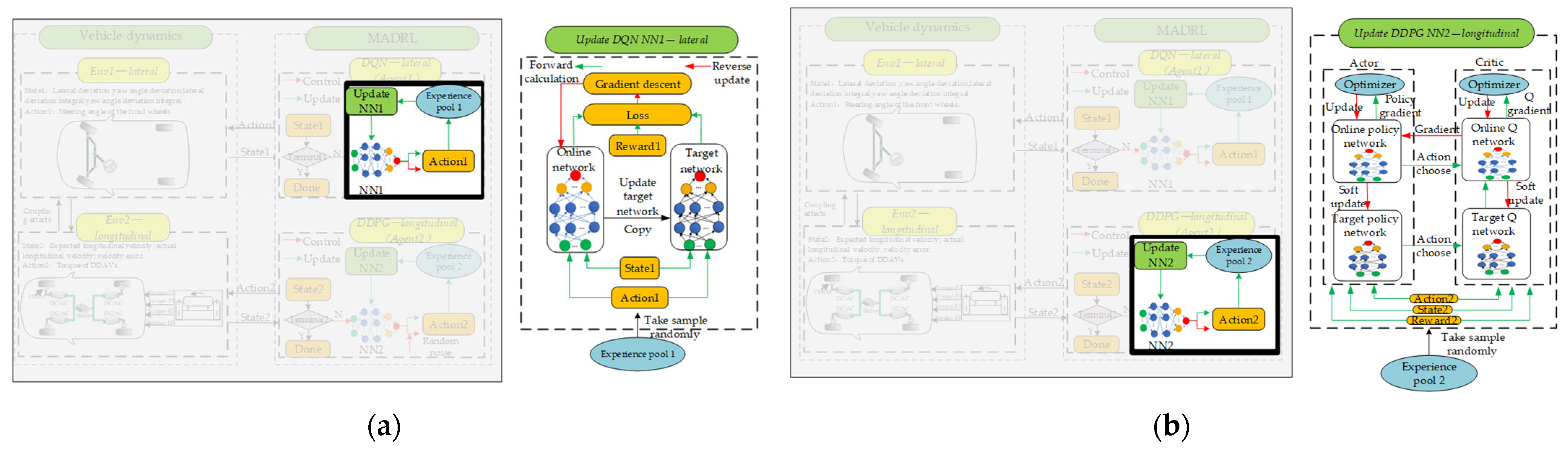
In this study, the updating processes of respective neural networks and the design of network frameworks are illustrated in Figure 6, Figure 7, Figure 8 and Figure 9. The settings of learning parameters for each agent and the definition of neural network structures are presented in Table 1 and Table 2.
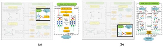
Figure 6.
(a) Process of the DQN neural network update. (b) Process of the DDPG neural network update.
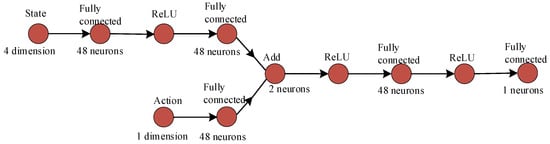
Figure 7.
Framework of DQN.

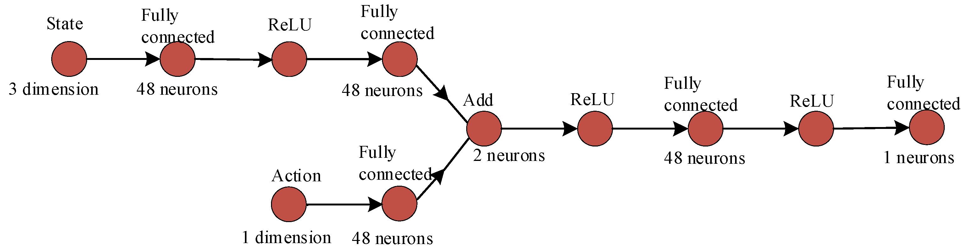
Figure 8.
Framework of The DDPG critic network.
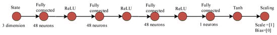
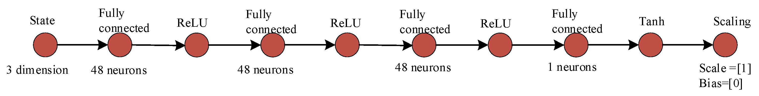
Figure 9.
Framework of the DDPG actor network.

Table 1.
Hyperparameters for DQN.
Table 2.
Hyperparameters for DDPG.
3. Results and Discussion
3.1. Training and Experimental Setup
In the Matlab/Simulink environment, the DDAV model and MADRL trajectory tracking control strategy were constructed. The training platform utilized the 11th Gen Intel(R) Core(TM) i7-1165G7 processor. The parameters of the DDAV are shown in Table 3. Considering the characteristics of the vehicle’s tires, scholars both domestically and internationally have proposed various tire dynamic models based on the nonlinear properties of tire dynamics, such as the “magic formula” semi-empirical tire model and the Dugoff tire model. The “magic formula” semi-empirical tire model demonstrates strong uniformity and high fitting accuracy, making it suitable for fields requiring precise descriptions of tire mechanics [35]. In this study, the vehicle tire model was constructed based on the “magic formula” semi-empirical tire model [36].
Table 3.
DDAV vehicle parameters.
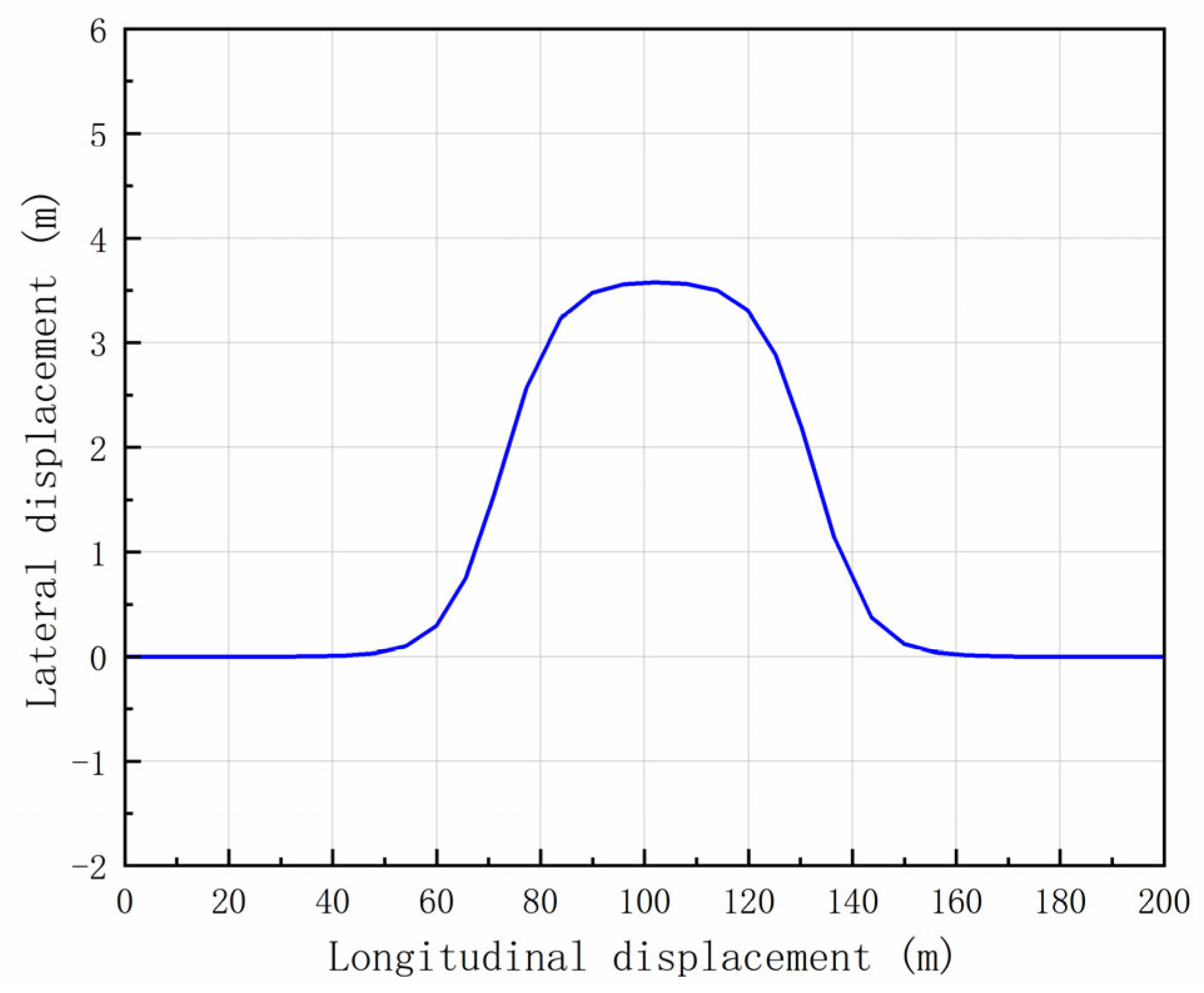
The double lane change (DLC) maneuver serves as a robust assessment of lane-keeping capabilities. Thus, a DLC scenario at a velocity of 36 km/h was selected for training purposes, with the reference trajectory depicted in Figure 10 [37]. To augment the adaptability of each intelligent agent, randomization of the initial lateral position deviation and initial longitudinal velocity deviation in the DDAV was performed at the onset of each training session.
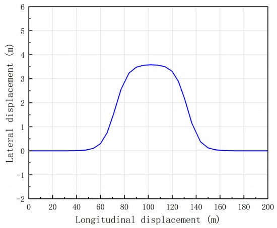
Figure 10.
Vehicle driving path for the learning process (DLC).
3.2. Iterative Training Results
The training objective of deep reinforcement learning is to maximize the reward value; thus, the indication of training completion lies in the stable convergence state of episode reward values after fluctuations. As depicted in Figure 11, longitudinal control shows the agent reaching stable convergence after the 1100th episode, whereas lateral control demonstrates stable convergence after the 200th episode.
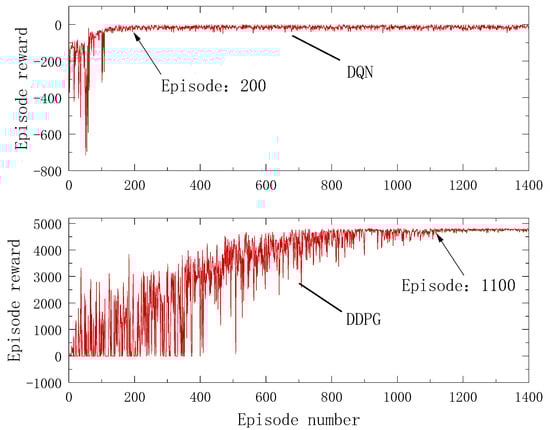
Figure 11.
Episode reward in the learning process.
3.3. Validation of Control Policy Effectiveness and Generalization
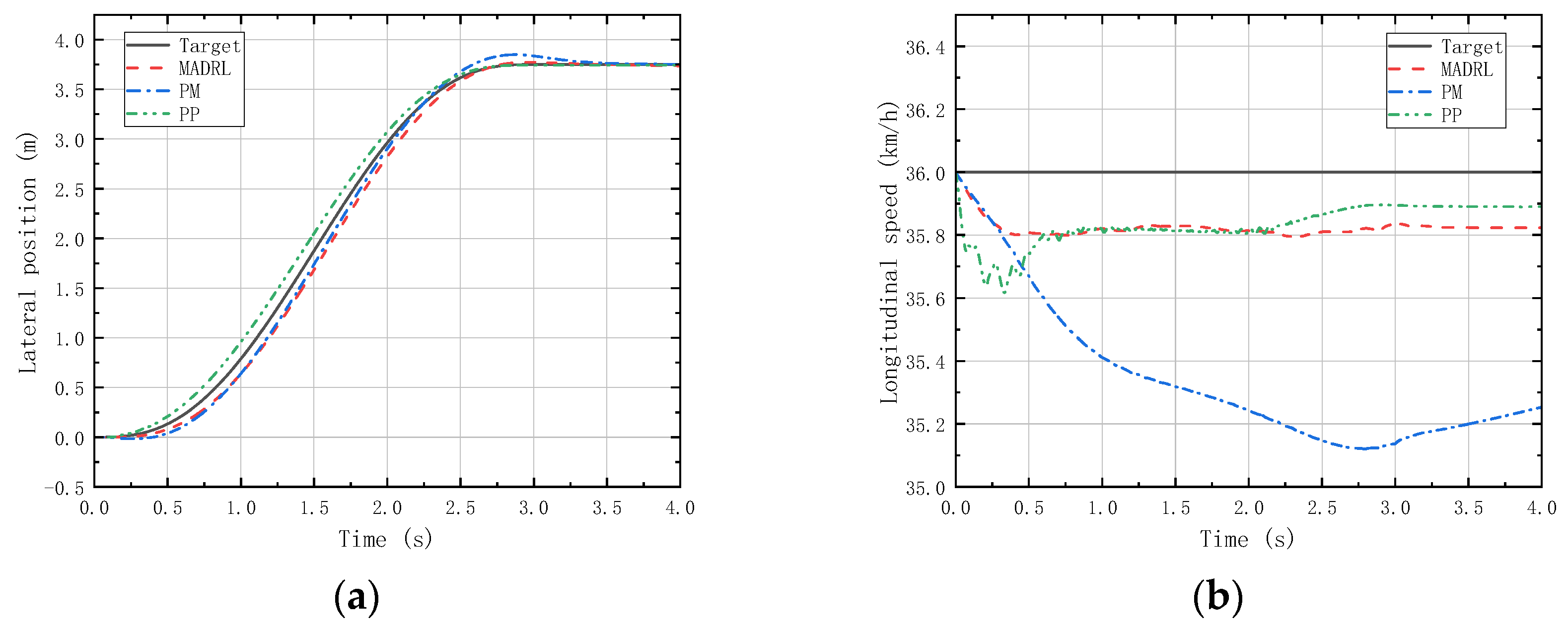
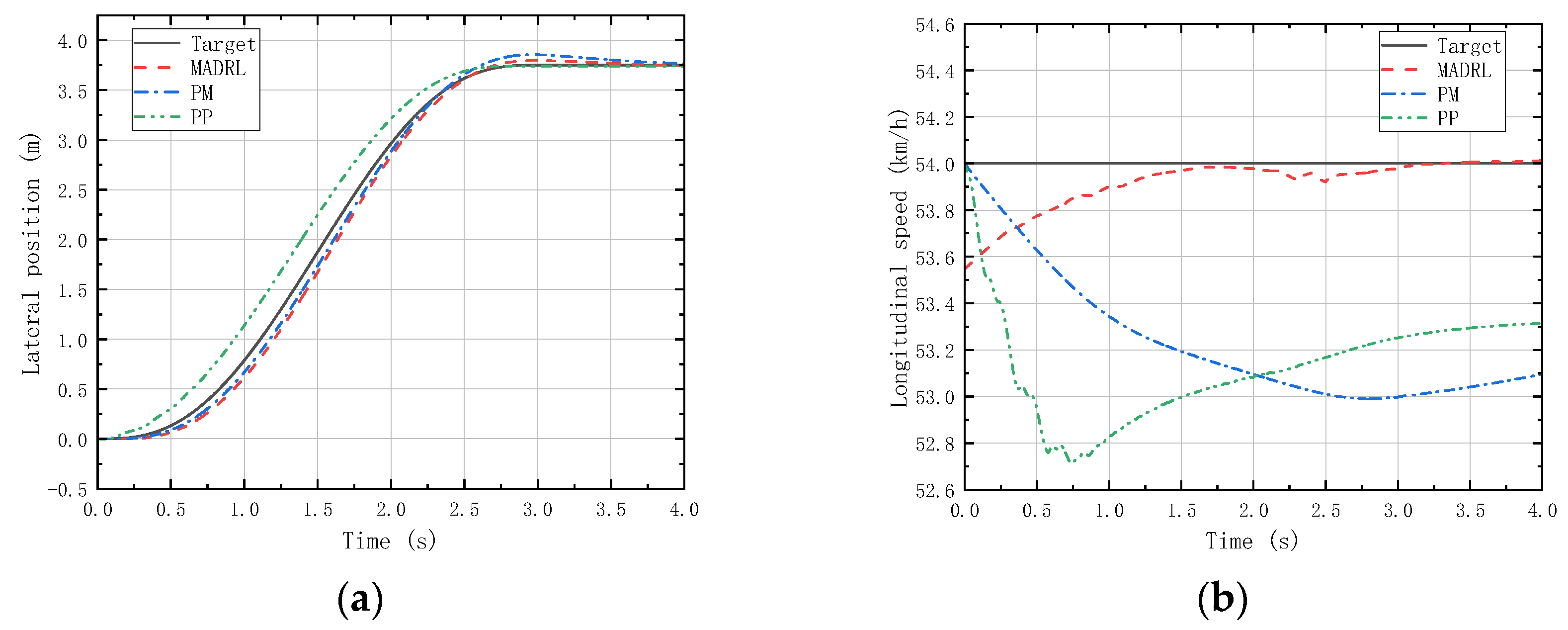
Trained agents were integrated into the control strategy to conduct lane-changing experiments and double lane-change experiments with the DDAV at a speed of 36 km/h. For the lane-changing operation (LC), adhering to the guidelines outlined in the “Urban Expressway Design Code of the People’s Republic of China (CJJ129-2009)”, a lane width of W = 3.75 m was utilized, with a designated completion time of 3 s for the lane-change maneuver. Two validated classical trajectory tracking longitudinal and lateral control methods were selected for comparison as follows: one method combines PID longitudinal velocity control with model predictive control (MPC) for lateral motion control (PM) [5,6], while the other combines PID longitudinal velocity control with pure tracking lateral motion control (PP) [7,8,9].
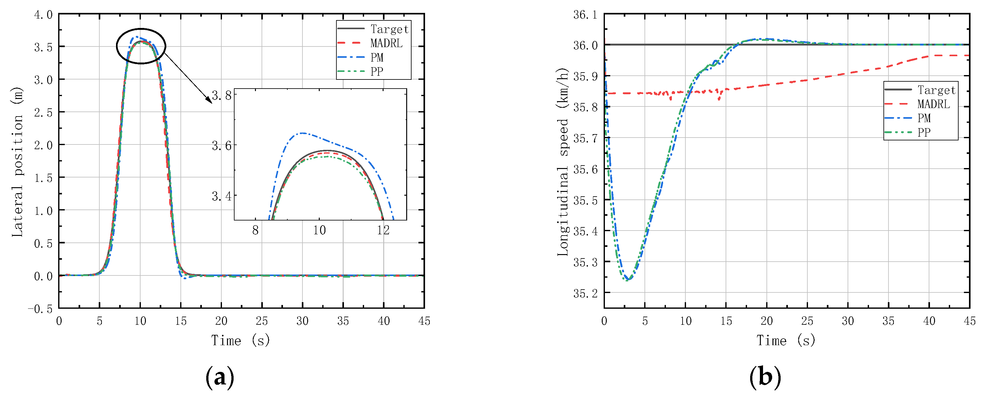
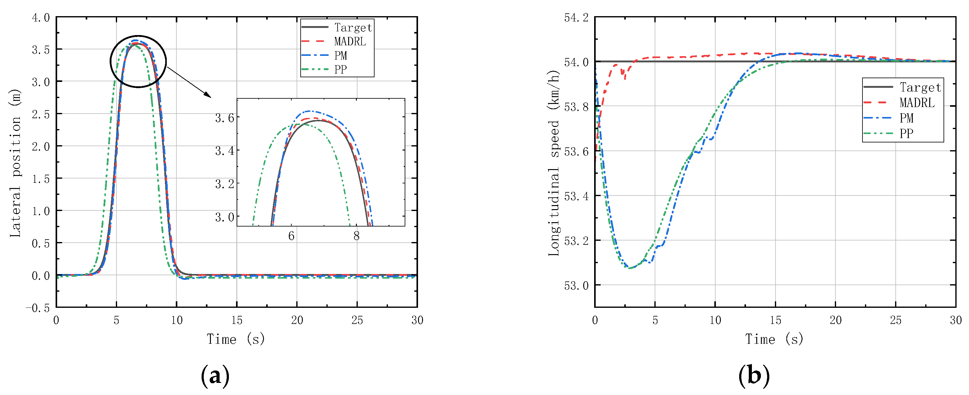
Figure 12 and Figure 13 respectively illustrate the lateral position and longitudinal velocity scenarios under LC and DLC experiments for both the MADRL method and classical control methods employed in this study.
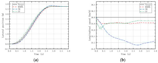
Figure 12.
(a) Vehicle lateral displacement (36 km/h-LC). (b) Vehicle tracking speed (36 km/h-LC).
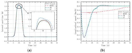
Figure 13.
(a) Vehicle lateral displacement (36 km/h-DLC). (b) Vehicle tracking speed (36 km/h-DLC).
Figure 12 shows that in the LC experiments, MADRL enables the vehicle to complete the LC maneuver more accurately within the specified time compared with classical control methods, with smaller lateral overshoot and maximum longitudinal velocity deviation compared with classical control methods. Figure 13 reveals that in the DLC experiments, MADRL exhibits a smaller maximum lateral position deviation and better robustness in longitudinal velocity. The deviation between longitudinal velocity and the desired longitudinal velocity remains consistently low, with a maximum longitudinal velocity deviation not exceeding 0.14 km/h, and the longitudinal velocity deviation under stable vehicle operation does not exceed 0.04 km/h. Although MADRL exhibits extremely small deviations in longitudinal velocity under stable vehicle operation, this minimal deviation is due to constraints imposed by the characteristics of the reinforcement learning algorithm itself. Specifically, after achieving all the reward and penalty metrics in the reward function, the algorithm no longer actively pursues further optimization, as doing so would not lead to higher rewards or lower penalties for the intelligent agent.
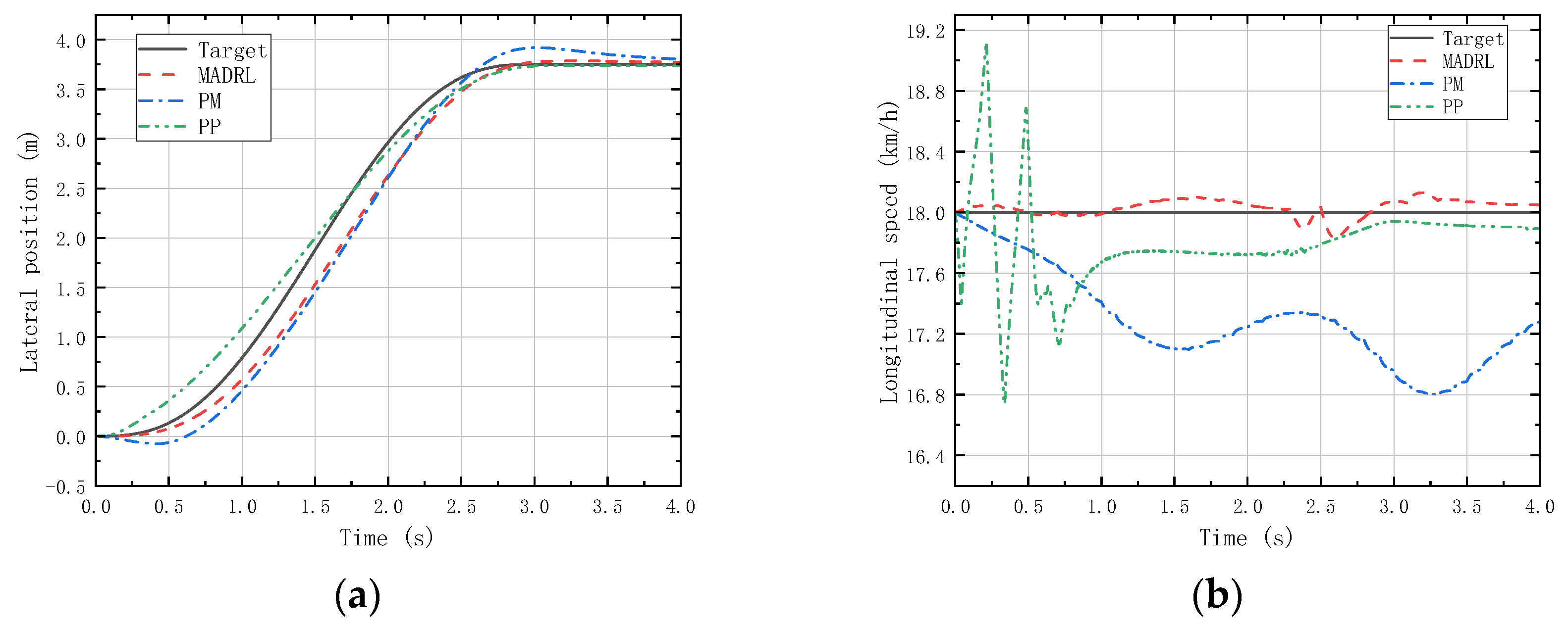
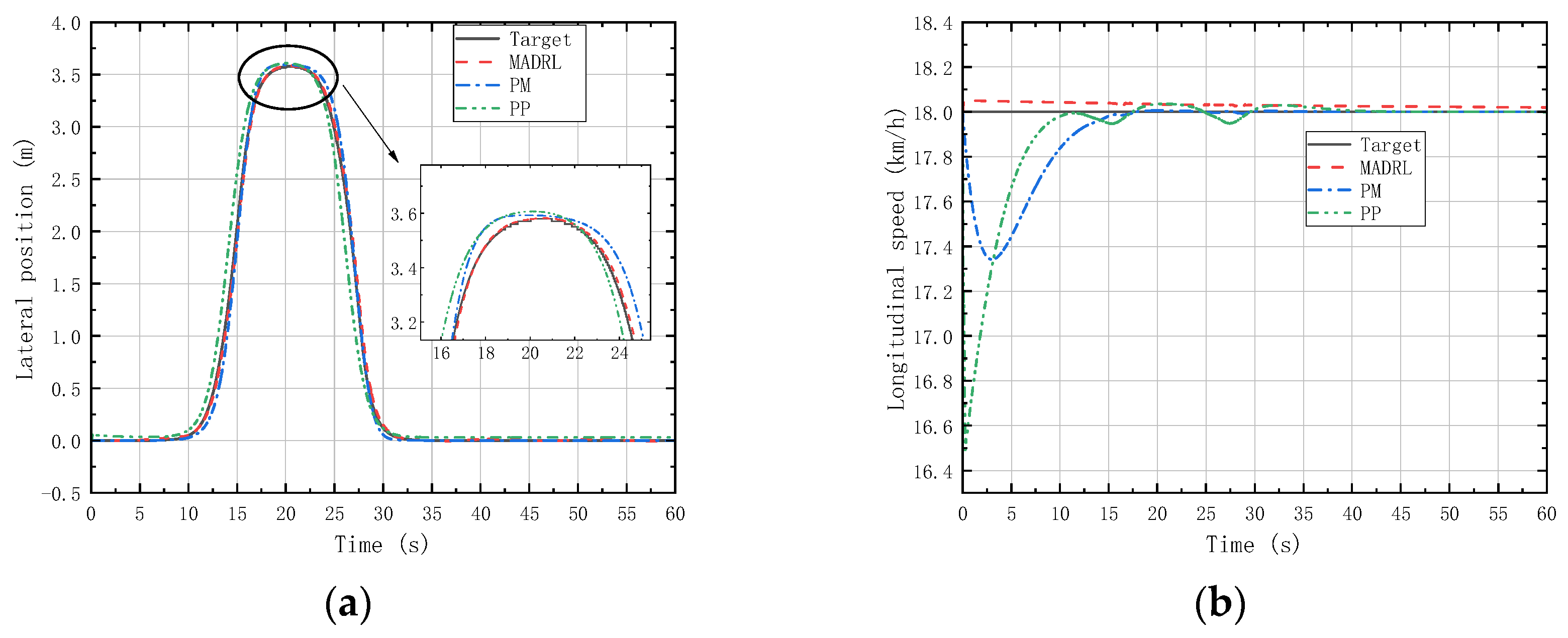
Additionally, we needed to verify the generalization capability of the trained control strategy at different speeds. Since the agents designed in this study pay more attention to the performance of lateral position deviation and velocity deviation, two moderate-speed states (18 km/h and 54 km/h) where vehicle instability is unlikely to occur were selected for generalization validation through LC and DLC experiments. Figure 14, Figure 15, Figure 16 and Figure 17 depict the lateral position and longitudinal velocity scenarios under LC and DLC experiments at different speeds for both the MADRL method and classical control methods employed in this study.
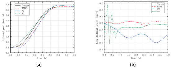
Figure 14.
(a) Vehicle lateral displacement (18 km/h-LC). (b) Vehicle tracking speed (18 km/h-LC).
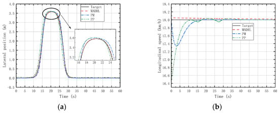
Figure 15.
(a) Vehicle lateral displacement (18 km/h-DLC). (b) Vehicle tracking speed (18 km/h-DLC).
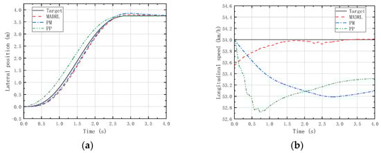
Figure 16.
(a) Vehicle lateral displacement (54 km/h-LC). (b) Vehicle tracking speed (54 km/h-LC).
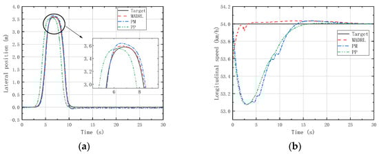
Figure 17.
(a) Vehicle lateral displacement (54 km/h-DLC). (b) Vehicle tracking speed (54 km/h-DLC).
Figure 14 and Figure 16 reveal that under LC experiments at different speeds, MADRL enables the vehicle to complete the lane-changing maneuver more accurately within the specified time, with a smaller lateral overshoot. Moreover, the maximum longitudinal velocity deviation for the MADRL method is consistently lower than that for classical control methods across all speed conditions. On the other hand, Figure 15 and Figure 17 demonstrate that under DLC experiments at different speeds, MADRL exhibits smaller maximum lateral position deviation and better robustness in longitudinal velocity. The deviation between longitudinal velocity and the desired longitudinal velocity remains consistently low. Specifically, during DLC experiments at 18 km/h, the maximum longitudinal velocity deviation for MADRL does not exceed 0.05 km/h, and under stable vehicle operation, the longitudinal velocity deviation does not exceed 0.02 km/h. Similarly, during DLC experiments at 54 km/h, the maximum longitudinal velocity deviation for MADRL does not exceed 0.4 km/h, and under stable vehicle operation, the longitudinal velocity deviation does not exceed 0.01 km/h (Table 4).
Table 4.
Comparison of the performance of DLC conditions.
The results above indicate that the MADRL method employed in this study, along with its corresponding design of intelligent agent reward and penalty functions, exhibits superior performance. The trained control policies demonstrate a certain degree of generalization capability across different speed scenarios. Under various operating conditions, the maximum lateral position deviation outperforms classical control methods, while the maximum longitudinal velocity deviation remains lower than that of classical control methods. Moreover, under stable vehicle operation, the longitudinal velocity deviation is minimal and within an acceptable range.
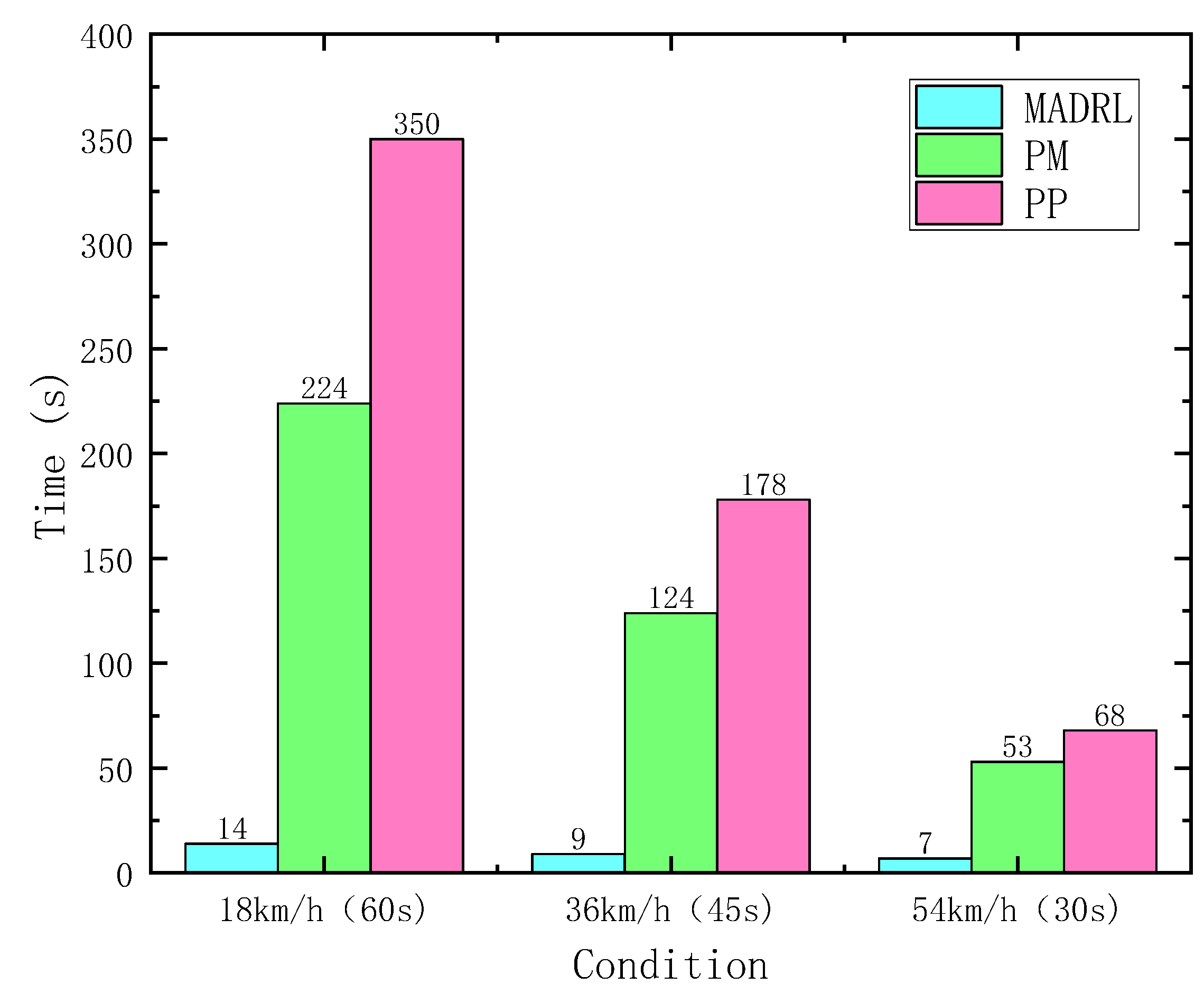
On the other hand, computational efficiency stands as a significant indicator for assessing the performance of strategy algorithms. The time consumption for different control strategies during the operation of DDAVs in a dual-lane change scenario is illustrated in Figure 18. When conducting a 60 s DLC experiment at 18 km/h, the time consumed by MADRL is approximately 6% of that by PM and 4% of that by PP. At 36 km/h for a 45 s DLC experiment, MADRL consumes approximately 7% of PM’s time and 5% of PP’s time. Likewise, at 54 km/h for a 30 s DLC experiment, MADRL consumes approximately 13% of PM’s time and 10% of PP’s time. Hence, the trajectory tracking control method based on MADRL in this study exhibits higher computational efficiency and lower computational resource requirements compared with classical control methods.

Figure 18.
Time spent under different simulations of DLC.
4. Conclusions
This study focuses on DDAV and proposes a MADRL control method for autonomous driving trajectory tracking. The DDPG algorithm is employed for longitudinal control, while the DQN algorithm is utilized for lateral control. Guided by optimization principles, lower-level torque allocation is integrated, enabling iterative training to achieve DDAV trajectory tracking control. The specific conclusions are as follows: The MADRL method in this study enables more accurate tracking of desired longitudinal velocity and lateral position by vehicles. Additionally, the trained intelligent agent networks demonstrate good generalization capability. In lane-changing and dual-lane change experiments under different speed conditions, the maximum longitudinal velocity deviation, maximum lateral position deviation, and lateral overshoot are lower than those of classical control methods. The maximum lateral position deviation is improved by up to 90.5%, and the maximum longitudinal velocity deviation is improved by up to 97%. Moreover, the MADRL method in this study significantly improves computational efficiency, saving computational resources. Compared with classical control methods, the running time in dual-lane change experiments under different speed conditions can be reduced by up to 93.7%.
In summary, compared with classical control methods, the DDAV trajectory tracking control method based on MADRL in this study exhibits greater adaptability, better robustness, higher computational efficiency, and good generalization. Furthermore, the application of DRL in actual vehicle operation for continuous training and periodic policy iteration throughout the lifecycle significantly reduces reliance on high-precision vehicle mathematical models and high computational resources compared with mainstream control methods. This approach is beneficial for the development and application of advanced control strategies for intelligent driving vehicles. However, DRL endows machines with a certain degree of autonomy in understanding, learning, and decision-making. Nonetheless, advanced intelligent driving cannot disregard the necessity of driver operation under certain conditions, namely, the human–machine co-driving issue in the process of intelligent driving. Especially when external environmental changes occur, introducing human intervention may be necessary, as machines may not be able to react promptly. Confronting such issues in complex environments necessitates the integration of human intelligence with machine intelligence. Promising directions for future research include identifying how to incorporate human judgment and experience in a timely manner based on MADRL, adopting more advanced algorithms such as DDQN and PPO, integrating human and machine intelligence, enhancing the capability of human–machine interactions, and achieving superior human–machine co-driving coordination.
Author Contributions
Conceptualization, Y.L. and W.D.; formal analysis, M.Y.; investigation, Y.L.; methodology, Y.L. and L.L.; resources, M.Y.; supervision, W.D. and M.Y.; validation, Y.L., H.Z. and L.L.; visualization, H.Z. and T.J.; writing—original draft, Y.L.; writing—review and editing, Y.L., T.J. and W.D. All authors have read and agreed to the published version of the manuscript.
Funding
This research was supported by the Natural Science Foundation of Sichuan Province under grant/award number 2023NSFSC0395 and Southwest Jiaotong University New Interdisciplinary Cultivation Fund under grant/award number 2682023ZLPY001.
Data Availability Statement
Data are available from authors on reasonable request.
Conflicts of Interest
The authors declare no conflicts of interest.
Nomenclature
| vehicle mass | |
| tire rolling radius | |
| vehicle center of mass height | |
| wheel rotational inertia | |
| road friction coefficient | |
| adhesion coefficient | |
| dc drag coefficient | |
| longitudinal force of the tire | |
| lateral force of the tire | |
| vertical load on the driving wheel | |
| longitudinal velocity of the vehicle | |
| lateral velocity of the vehicle | |
| yaw rate of the vehicle | |
| yaw inertia coefficient of the vehicle | |
| average front wheel steering angle of the vehicle | |
| sideslip angle of the vehicle | |
| and | distances from the center of gravity to the front and rear axles |
| forward speed of the vehicle | |
| half of the wheelbase | |
| expected lateral position of the vehicle at the given moment | |
| actual lateral position of the vehicle at that moment | |
| expected yaw angle of the vehicle at the given moment | |
| actual yaw angle of the vehicle at that moment | |
| lateral position deviation of the vehicle | |
| yaw angle deviation of the vehicle | |
| respective rates of | |
| respective rates of | |
| front wheel steering command | |
| desired longitudinal velocity of the vehicle | |
| deviation of desired and actual longitudinal velocity | |
| accelerations or decelerations of the vehicle | |
| the torque commands sent to each driving motor |
References
- Jin, T.; Ding, W.; Yang, M.; Zhu, H.; Dai, P. Benchmarking Perception to Streaming Inputs in Vision-Centric Autonomous Driving. Mathematics 2023, 11, 4976. [Google Scholar] [CrossRef]
- Jin, T.; Zhang, C.; Zhang, Y.; Yang, M.; Ding, W. A Hybrid Fault Diagnosis Method for Autonomous Driving Sensing Systems Based on Information Complexity. Electronics 2024, 13, 354. [Google Scholar] [CrossRef]
- Lin, F.; Zhang, Y.; Zhao, Y.; Yin, G.; Zhang, H.; Wang, K. Trajectory tracking of autonomous vehicle with the fusion of DYC and longitudinal–lateral control. Chin. J. Mech. Eng. 2019, 32, 1–16. [Google Scholar] [CrossRef]
- Cremean, L.B.; Foote, T.B.; Gillula, J.H.; Hines, G.H.; Kogan, D.; Kriechbaum, K.L.; Lamb, J.C.; Leibs, J.; Lindzey, L.; Rasmussen, C.E. Alice: An information-rich autonomous vehicle for high-speed desert navigation. J. Field Robot. 2006, 23, 777–810. [Google Scholar] [CrossRef]
- Diab, M.K.; Ammar, H.H.; Shalaby, R.E. Self-driving car lane-keeping assist using pid and pure pursuit control. In Proceedings of the 2020 International Conference on Innovation and Intelligence for Informatics, Computing and Technologies (3ICT), Sakheer, Bahrain, 20–21 December 2020; pp. 1–6. [Google Scholar]
- Srinivas, C.; Patil, S.S. A Waypoint Tracking Controller for Autonomous Vehicles Using CARLA Simulator. In Recent Advances in Hybrid and Electric Automotive Technologies: Select Proceedings of HEAT 2021; Springer: Berlin/Heidelberg, Germany, 2022; pp. 197–206. [Google Scholar]
- Samak, C.V.; Samak, T.V.; Kandhasamy, S. Control strategies for autonomous vehicles. In Autonomous Driving and Advanced Driver-Assistance Systems (ADAS); CRC Press: Boca Raton, FL, USA, 2021; pp. 37–86. [Google Scholar]
- Chen, S.; Chen, H. MPC-based path tracking with PID speed control for autonomous vehicles. In Proceedings of the IOP Conference Series: Materials Science and Engineering, Hangzhou, China, 18–20 April 2020; p. 012034. [Google Scholar]
- Samuel, M.; Mohamad, M.; Hussein, M.; Saad, S.M. Lane keeping maneuvers using proportional integral derivative (PID) and model predictive control (MPC). J. Robot. Control (JRC) 2021, 2, 78–82. [Google Scholar] [CrossRef]
- Nie, L.; Guan, J.; Lu, C.; Zheng, H.; Yin, Z. Longitudinal speed control of autonomous vehicle based on a self-adaptive PID of radial basis function neural network. IET Intell. Transp. Syst. 2018, 12, 485–494. [Google Scholar] [CrossRef]
- Jo, A.; Lee, H.; Seo, D.; Yi, K. Model-reference adaptive sliding mode control of longitudinal speed tracking for autonomous vehicles. Proc. Inst. Mech. Eng. Part D J. Automob. Eng. 2023, 237, 493–515. [Google Scholar] [CrossRef]
- Dahiwale, P.B.; Chaudhari, M.A.; Kumar, R.; Selvaraj, G. Model Predictive Longitudinal Control for Autonomous Driving. In Proceedings of the 2023 IEEE 3rd International Conference on Sustainable Energy and Future Electric Transportation (SEFET), Bhubaneswar, India, 9–12 August 2023; pp. 1–6. [Google Scholar]
- Hang, P. Longitudinal Velocity Tracking Control of a 4WID Electric Vehicle. IFAC-Pap. 2018, 51, 790–795. [Google Scholar] [CrossRef]
- Han, G.; Fu, W.; Wang, W.; Wu, Z. The lateral tracking control for the intelligent vehicle based on adaptive PID neural network. Sensors 2017, 17, 1244. [Google Scholar] [CrossRef]
- Park, M.-W.; Lee, S.-W.; Han, W.-Y. Development of lateral control system for autonomous vehicle based on adaptive pure pursuit algorithm. In Proceedings of the 2014 14th International Conference on Control, Automation and Systems (ICCAS 2014), Gyeonggi-do, Republic of Korea, 22–25 October 2014; pp. 1443–1447. [Google Scholar]
- Chen, G.; Yao, J.; Hu, H.; Gao, Z.; He, L.; Zheng, X. Design and experimental evaluation of an efficient MPC-based lateral motion controller considering path preview for autonomous vehicles. Control Eng. Pract. 2022, 123, 105164. [Google Scholar] [CrossRef]
- Huang, H.; Huang, X.; Ding, W.; Yang, M.; Yu, X.; Pang, J. Vehicle vibro-acoustical comfort optimization using a multi-objective interval analysis method. Expert Syst. Appl. 2023, 213, 119001. [Google Scholar] [CrossRef]
- Huang, H.; Lim, T.C.; Wu, J.; Ding, W.; Pang, J. Multitarget prediction and optimization of pure electric vehicle tire/road airborne noise sound quality based on a knowledge-and data-driven method. Mech. Syst. Signal Process. 2023, 197, 110361. [Google Scholar] [CrossRef]
- Huang, H.; Huang, X.; Ding, W.; Yang, M.; Fan, D.; Pang, J. Uncertainty optimization of pure electric vehicle interior tire/road noise comfort based on data-driven. Mech. Syst. Signal Process. 2022, 165, 108300. [Google Scholar] [CrossRef]
- Gueriani, A.; Kheddar, H.; Mazari, A.C. Deep Reinforcement Learning for Intrusion Detection in IoT: A Survey. In Proceedings of the 2023 2nd International Conference on Electronics, Energy and Measurement (IC2EM), Medea, Algeria, 28–29 November 2023; pp. 1–7. [Google Scholar]
- Karalakou, A.; Troullinos, D.; Chalkiadakis, G.; Papageorgiou, M. Deep Reinforcement Learning Reward Function Design for Autonomous Driving in Lane-Free Traffic. Systems 2023, 11, 134. [Google Scholar] [CrossRef]
- Li, D.; Okhrin, O. Vision-Based DRL Autonomous Driving Agent with Sim2Real Transfer. In Proceedings of the 2023 IEEE 26th International Conference on Intelligent Transportation Systems (ITSC), Bilbao, Spain, 28–29 November 2023; pp. 866–873. [Google Scholar]
- Ashwin, S.H.; Naveen Raj, R. Deep reinforcement learning for autonomous vehicles: Lane keep and overtaking scenarios with collision avoidance. Int. J. Inf. Tecnol. 2023, 15, 3541–3553. [Google Scholar] [CrossRef]
- Vimal Kumar, A.R.; Theerthala, R.R. Reinforcement Learning based Parking Space Egress for Autonomous Driving; SAE Technical Paper: Warrendale, PA, USA, 2024; ISSN 0148-7191. [Google Scholar]
- Fu, Y.; Li, C.; Yu, F.R.; Luan, T.H.; Zhang, Y. A decision-making strategy for vehicle autonomous braking in emergency via deep reinforcement learning. IEEE Trans. Veh. Technol. 2020, 69, 5876–5888. [Google Scholar] [CrossRef]
- Wei, H.; Zhang, N.; Liang, J.; Ai, Q.; Zhao, W.; Huang, T.; Zhang, Y. Deep reinforcement learning based direct torque control strategy for distributed drive electric vehicles considering active safety and energy saving performance. Energy 2022, 238, 121725. [Google Scholar] [CrossRef]
- Lin, X.; Ye, Z.; Zhou, B. DQN Reinforcement Learning-based Steering Control Strategy for Autonomous Driving. J. Mech. Eng. 2023, 59, 315–324. [Google Scholar]
- Yao, J.; Ge, Z. Path-Tracking Control Strategy of Unmanned Vehicle Based on DDPG Algorithm. Sensors 2022, 22, 7881. [Google Scholar] [CrossRef]
- Abe, M. Vehicle Handling Dynamics: Theory and Application; Butterworth-Heinemann: Oxford, UK, 2015. [Google Scholar]
- Lim, E.H.; Hedrick, J.K. Lateral and longitudinal vehicle control coupling for automated vehicle operation. In Proceedings of the 1999 American Control Conference (Cat. No. 99CH36251), San Diego, CA, USA, 2–4 June 1999; pp. 3676–3680. [Google Scholar]
- Han, P.; Zhang, B. Path planning and trajectory tracking strategy of autonomous vehicles. Math. Probl. Eng. 2021, 2021, 8865737. [Google Scholar] [CrossRef]
- Buşoniu, L.; Babuška, R.; De Schutter, B. Multi-agent reinforcement learning: An overview. Innov. Multi-Agent Syst. Appl. 2010, 1, 183–221. [Google Scholar]
- Zhang, S.-L.; Wen, C.-K.; Ren, W.; Luo, Z.-H.; Xie, B.; Zhu, Z.-X.; Chen, Z.-J. A joint control method considering travel speed and slip for reducing energy consumption of rear wheel independent drive electric tractor in ploughing. Energy 2023, 263, 126008. [Google Scholar] [CrossRef]
- Xiong, J.; Wang, Q.; Yang, Z.; Sun, P.; Han, L.; Zheng, Y.; Fu, H.; Zhang, T.; Liu, J.; Liu, H. Parametrized deep q-networks learning: Reinforcement learning with discrete-continuous hybrid action space. arXiv 2018, arXiv:1810.06394. [Google Scholar]
- Pacejka, H. Tire and Vehicle Dynamics; Elsevier: Amsterdam, The Netherlands, 2005. [Google Scholar]
- Burhaumudin, M.S.; Samin, P.M.; Jamaluddin, H.; Rahman, R.; Sulaiman, S. Modeling and validation of magic formula tire model. In Proceedings of the International Conference on the Automotive Industry, Mechanical and Materials Science (ICAMME’2012), Penang, Malaysia, 19 May 2012; pp. 113–117. [Google Scholar]
- Ji, X.; He, X.; Lv, C.; Liu, Y.; Wu, J. Adaptive-neural-network-based robust lateral motion control for autonomous vehicle at driving limits. Control Eng. Pract. 2018, 76, 41–53. [Google Scholar] [CrossRef]


Disclaimer/Publisher’s Note: The statements, opinions and data contained in all publications are solely those of the individual author(s) and contributor(s) and not of MDPI and/or the editor(s). MDPI and/or the editor(s) disclaim responsibility for any injury to people or property resulting from any ideas, methods, instructions or products referred to in the content. |
© 2024 by the authors. Licensee MDPI, Basel, Switzerland. This article is an open access article distributed under the terms and conditions of the Creative Commons Attribution (CC BY) license (https://creativecommons.org/licenses/by/4.0/).