Abstract
This work proposes an innovative approach to enhance the localization of unmanned aerial vehicles (UAVs) in dynamic environments. The methodology integrates a sophisticated object-tracking algorithm to augment the established simultaneous localization and mapping (ORB-SLAM) framework, utilizing only a monocular camera setup. Moving objects are detected by harnessing the power of YOLOv4, and a specialized Kalman filter is employed for tracking. The algorithm is integrated into the ORB-SLAM framework to improve UAV pose estimation by correcting the impact of moving elements and effectively removing features connected to dynamic elements from the ORB-SLAM process. Finally, the results obtained are recorded using the TUM RGB-D dataset. The results demonstrate that the proposed algorithm can effectively enhance the accuracy of pose estimation and exhibits high accuracy and robustness in real dynamic scenes.
MSC:
68T45
1. Introduction
In recent years, unmanned aerial vehicles (UAVs), commonly known as drones, have undergone significant advancements due to technological breakthroughs that have enhanced their design and functionality. This evolution has expanded their practical applications across various sectors, significantly improving their operational efficiency and capabilities. In agriculture [1], UAVs are indispensable for precise crop mapping, real-time harvest analyses, and early pest detection, leading to better crop management strategies. In search and rescue operations [2], drones quickly cover large areas, locate distressed individuals, and provide crucial information in disaster-stricken areas. The military sector benefits from UAVs through advanced reconnaissance and immediate intelligence [3], revolutionizing modern warfare and strategy. At the same time, in environmental conservation, they respond swiftly to forest fires, conduct air quality studies, and track wildlife [4].
Commercially, UAVs have transformed business methodologies by offering a safer, more cost-effective alternative to manned aerial data collection [5] compatible with diverse payloads like high-resolution cameras and sensor arrays. This adaptability hints at future developments such as enhanced autonomous navigation and sophisticated delivery systems. Additionally, UAVs are becoming crucial to urban development, promising to improve traffic management, urban planning, and public safety in Smart Cities [6,7,8]. They are also set to revolutionize the transportation industry by introducing drone taxis and automated delivery services [9], indicating a significant shift in urban mobility and logistics. Regulatory bodies are changing policies to balance the benefits of UAVs against privacy and security concerns, ensuring their smooth and beneficial integration into society.
However, as with any emerging technology, UAVs face challenges in maintaining precision and dependability while performing autonomous tasks in real-world settings, particularly in regions with weak or nonexistent GPS signals. One methodology involves the application of SLAM, which leverages optical data to discern features, thereby enabling the real-time determination of a UAV’s trajectory and spatial orientation while simultaneously facilitating the generation of a navigational map [10]. A supplementary strategy integrates visual sensing with laser and/or inertial measurement units to enhance locational accuracy [11]. Additionally, deploying GNSS-augmented LiDAR systems offers a robust alternative via the augmentation of positional data with high-fidelity topographical information [12]. Another approach merges the functionalities of optical sensors with LiDAR technology, capitalizing on the complementary strengths of both systems to refine navigational precision [13]. However, these techniques, which use multiple sensors, can become costly and cumbersome when used in applications like low-cost drones or in scenarios such as city surveillance in which weight restrictions are imposed. They pose challenges as they are sometimes memory-intensive and time-consuming, requiring more powerful processing to run in real time.
In response to these challenges, efforts have been made to explore alternative navigation techniques, such as visual SLAM (VSLAM), that are used only on sensor monocular cameras. Most visual SLAM systems are designed to operate in static environments, leading to error accumulation when environmental changes occur. This reduces the accuracy and reliability of these systems. Recent advancements in machine learning [14] have spurred the development of new visual SLAM approaches that incorporate deep learning to address these dynamic issues. Notably, SLAM methods now increasingly incorporate object detection algorithms such as YOLO to identify dynamic objects within a scene.
Using YOLO for object detection helps create precise and real-time tracking systems by accurately identifying and categorizing dynamic elements in an environment. This is particularly effective in environments in which the contours of dynamic objects are usually clear and distinct from static backgrounds. This clarity aids in refining the detection outlines of dynamic objects, enhancing the overall performance of the SLAM system. Moreover, its robustness in varying lighting and weather conditions enhances its utility in outdoor applications. However, challenges persist due to the limited diversity of recognizable objects and the size of the training dataset. These limitations can result in incomplete coverage of dynamic objects, thereby reducing the number of dynamic objects detected in scenes. Consequently, these objects may not be accurately filtered out of the SLAM process, thereby affecting the correct estimation of the camera’s position and the mapping of its surroundings.
To address the aforementioned issues and enhance the accuracy and robustness of pose estimation in visual SLAM systems operating within dynamic indoor environments, the primary contributions of the proposed method are outlined as follows:
- (1)
- The capabilities of YOLOv4 are leveraged to accurately identify and classify various objects in images or videos. Additionally, a specific Kalman filter that utilizes the centroids of objects for enhanced tracking accuracy is integrated.
- (2)
- An algorithm has been developed to selectively filter features associated with dynamic objects.
- (3)
- These object detection and tracking models are integrated into the ORB-SLAM process. This integration involves deleting feature information from dynamic objects to prevent them from adversely affecting the SLAM performance. This approach ensures that the system can more effectively navigate and map environments in which object movement occurs using only a monocular camera.
In the following sections, existing studies pertinent to this challenge are examined, this study’s approach is outlined, and the findings of this study are delved into. The technique is applied to a widely recognized dataset to evaluate the extent of improvements made by the proposed methods.
2. Related Work
This section offers a concise summary of the research topics explored in this paper. Firstly, monocular SLAM is explored in the context of its application to UAVs. This part delves into the specifics of using monocular SLAM, discussing its development, its application in UAVs, and how it differs from other SLAM techniques such as stereo or LiDAR-based SLAM. Secondly, the integration of SLAM and object tracking for UAV localization is examined. This discussion focuses on recent works demonstrating how combining SLAM and object tracking can enhance UAV localization.
2.1. Monocular SLAM in UAVs
SLAM has been a focal point of research for many years and has recently sparked increased interest due to its application in fields like autonomous vehicle navigation in the automotive industry [15]. A number of methods can be used to create effective SLAM based on the specific type of sensor utilized for position determination and environmental mapping. The literature [16] presents solutions integrating visual (RGB) and inertial sensors. However, significant interest remains in visual SLAM (vSLAM) approaches in which either monocular or stereo cameras are employed in real time to concurrently map the environment and pinpoint the camera’s location. In this paper, our focus is restricted to monocular SLAM as it currently provides the most lightweight option suitable for integration into small UAVs. This approach aligns with the objective to develop a low-cost drone for surveillance missions. Additionally, the choice is influenced by the European regulatory framework, which limits the weight of autonomous drones to 900 g, particularly for UAVs operating near people [17]. Within the field of visual monocular SLAM, there are two leading state-of-the-art methodologies as feature-based and direct techniques. Feature-based methods, exemplified by algorithms like ORB-SLAM, as mentioned in Reference [18], focus on extracting feature details from each image frame, such as blobs and corners. These features are then used to achieve mapping and localization by tracking their positions across successive frames. An example of a high-speed algorithm in this category is provided by Artal et al. [10].
Conversely, direct methods adopt an alternative strategy, as detailed in Reference [19]. A prominent example of this is the Large-Scale Direct SLAM (LSD-SLAM) method [20]. Unlike feature-based methods, direct methods use the entire dataset in an image, compare complete images to reference them, and use image intensities to obtain information about the location and map [21]. This comprehensive data usage provides direct methods higher levels of robustness and accuracy. However, this comes at the cost of an increased computational demand, especially when compared to the efficiency of feature-based methods like ORB-SLAM. There are also combined techniques; for example, semi-direct SLAM is combined with feature-based SLAM [22].
2.2. Dynamic SLAM
In the field of UAV localization, SLAM is of paramount importance, especially in dynamic environments in which the behavior of moving objects presents significant challenges [23]. Dynamic objects, which are characterized by their unpredictable motion and changing appearances, complicate the task of accurate navigation and mapping. To address these complexities, the integration of object tracking with SLAM has emerged as an effective solution [24]. This combination enhances the ability of UAVs to accurately perceive and navigate their surroundings by continuously adapting to changes in the environment, thus ensuring more reliable and precise localization in various operational contexts.
In this scenario, the research presented in [25] unveils an innovative mapping technique that integrates the ORB-SLAM2 algorithm with the YOLOv5 (You Only Look Once) network. The function of the YOLOv5 network is to identify dynamic objects in each frame of a video followed by the exclusion of dynamic feature points, with the aim of improving the precision and dependability of the SLAM procedure. This method marks a substantial progression in tackling the difficulties associated with dynamic settings in UAV localization.
Meanwhile, Ref. [26] details a novel approach to SLAM in dynamic environments that utilizes a machine learning algorithm for tracking moving objects. This research employs a blend of LiDAR and camera sensors to determine the presence of objects and obtain depth data in real time. It introduces an inventive variation of the RANSAC methodology, known as multilevel RANSAC (ML-RANSAC), which is incorporated into an extended Kalman filter (EKF) setup for tracking multiple targets (MTT). The extended Kalman filter incorporates the robot’s model for improved tracking performance.
In [27], the DynaSLAM system is presented, which enhances tracking, mapping, and inpainting in dynamically populated environments. This system merges dynamic object detection with background inpainting within the ORB-SLAM framework, a renowned visual SLAM architecture. Tailored for dynamic environments, it supports various camera setups including monocular, stereo, and RGB-D configurations. DynaSLAM’s versatility enables effective mapping and localization in environments undergoing significant changes.
Conversely, Ref. [28] presents a technique that combines the Visual–Inertial Navigation System (VINS) with dynamic object detection to enhance the accuracy of autonomous vehicles functioning in dynamic environments. The method employs the YOLOv5 network for dynamic object recognition, disregards feature points within these objects’ vicinities, and models GPS data as general factors to mitigate cumulative errors. The approach is validated and demonstrates its efficacy in reducing the influence of moving objects and accumulating navigational errors, thereby offering improved navigational guidance for autonomous vehicles.
Reference [29] introduces Dynam-SLAM, a stereo visual–inertial SLAM system designed to perform effectively in highly dynamic environments. It achieves this by identifying and closely integrating dynamic and static features alongside an Inertial Measurement Unit (IMU) for nonlinear optimization.
The authors of [30] present a technique that establishes a mutually beneficial relationship between SLAM (simultaneous localization and mapping) and object detection. This technique incorporates deep learning-based object detection, effectively eliminating features associated with dynamic objects. Through this approach, the suggested framework empowers unmanned aerial vehicles (UAVs) to execute tasks adeptly in changing surroundings. Furthermore, it bolsters the capabilities of object detection systems, making them more proficient at handling demanding scenarios.
In Reference [31], the authors introduce an enhancement to visual odometry by leveraging the single-shot multibox detector (SSD) algorithm within dynamic settings, aiming to refine in pose estimation caused by data derived from mobile objects. The methodology integrates the SSD algorithm with optical flow methods to identify and eliminate dynamic feature points. These adjustments are subsequently merged with ORB-SLAM2, enhancing the precision of pose estimation.
Reference [32] presents a Distribution- and Local-based Random Sample Consensus (DLRSAC) algorithm crafted for isolating static features within dynamic environments. This is achieved by discerning inherent distinctions between moving and stationary elements.
3. Dynamic Object Tracking and Elimination
This research introduces a robust VSLAM algorithm tailored for UAV localization in dynamic settings which is mindful of the existence of moving objects [33]. This methodology is implemented using the ORB-SLAM algorithm, a monocular visual SLAM technique. To ensure its efficacy in dynamic settings, ORB-SLAM [34] is augmented with a YOLO-Kalman framework which merges YOLOv4, an object detection algorithm [35], with the Kalman filter, thereby enhancing localization and mapping.
The structure of the proposed approach is depicted in Figure 1. The blue component represents ORB-SLAM, while the orange component corresponds to the proposed object detection and tracking module. This module is integrated with ORB-SLAM to address dynamic objects. This schematic representation aims to help visualize the workflow and understand key steps in the ORB-SLAM process and the overall proposed methodology.
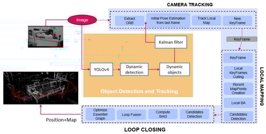
Figure 1.
The flowchart for ORB-SLAM and object tracking using a Kalman filter.
ORB-SLAM is a prevalent algorithm for conducting SLAM in 3D settings through the use of photographic sensors. It incorporates three main components: TRACKING, LOCAL MAPPING, and LOOP CLOSING. These elements collaboratively facilitate the real-time determination of a camera’s position, the creation of a local map, and the identification of loops to maintain the global map’s consistency.
3.1. Camera Tracking
The camera tracking component is crucial in determining the camera’s position in real time as it navigates through an environment. This involves initializing the camera’s position, selecting key images, extracting and matching features between the key images and the current image, estimating the camera’s position using the matches, and relocating if tracking is lost. The aim is to continuously track the camera’s position and orientation as accurately as possible.
3.2. Local Mapping
The local mapping component focuses on constructing a local map of the environment. It performs a variety of tasks, such as triangulating 3D points using correspondences between keyframes and the current image, eliminating redundant keyframes to optimize computational efficiency, adjusting the beam locally to fine-tune camera poses and map points, and updating the keyframe database to maintain a diverse set of keyframes for robust tracking and loop closure. The local map represents a portion of the environment around the camera’s trajectory.
3.3. Loop Closing
Loop closing is tasked with identifying and rectifying loop closures, situations in which the camera revisits a location it has encountered before. Its main aim is to ensure overall map consistency and reduce drift. Loop closure involves recognizing loop closure candidates by comparing the current image with key images in the database, checking loops for geometric consistency and appearance, performing a global bundle adjustment to optimize the overall map, and updating the covisibility graph representing relationships between key images to reflect newly detected loop closures. By closing loops, ORB-SLAM can correct accumulated errors and obtain a more accurate, globally consistent map.
3.4. Detecting and Tracking Objects
Detecting and tracking are based on two components: YOLOv4 and the Kalman filter.
YOLOv4is trained using the COCO (Common Objects in Context) dataset. This extensive dataset is utilized for tasks such as object detection, segmentation, and captioning. It encompasses more than 330,000 images with labels spread across more than 80 categories of objects, establishing it as a frequently employed standard in the study of object detection. The YOLOv4 algorithm identifies objects within images and videos, delivering high precision and rapid processing. It provides the coordinates for each object’s bounding box, specifies its category, and evaluates the detection confidence level. The classification of objects is crucial for recognizing and sorting moving objects that have been detected.
The Kalman filter is an algorithm that iteratively predicts a system’s state using noisy measurements. In this context, it continuously tracks an object’s position, even when measurements from the YOLO detector are unavailable. By integrating YOLOv4 with the Kalman filter, a robust system capable of effectively detecting and tracking objects in dynamic environments is created, complementing the ORB-SLAM algorithm.
Integrating deep learning technology and the Kalman tracking module within the ORB-SLAM framework enables real-time object detection and the elimination of dynamic objects. This configuration allows ORB-SLAM to monitor the camera’s motion and create a map of its surroundings, even within changing environments.
To facilitate an understanding of VSLAM techniques, including ORB-SLAM and the proposed VSLAM, refer to Figure 2, Figure 3 and Figure 4. These figures present detailed flowcharts illustrating simplified versions of the processes.
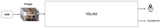
Figure 2.
Visual simultaneous localization and mapping.
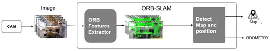
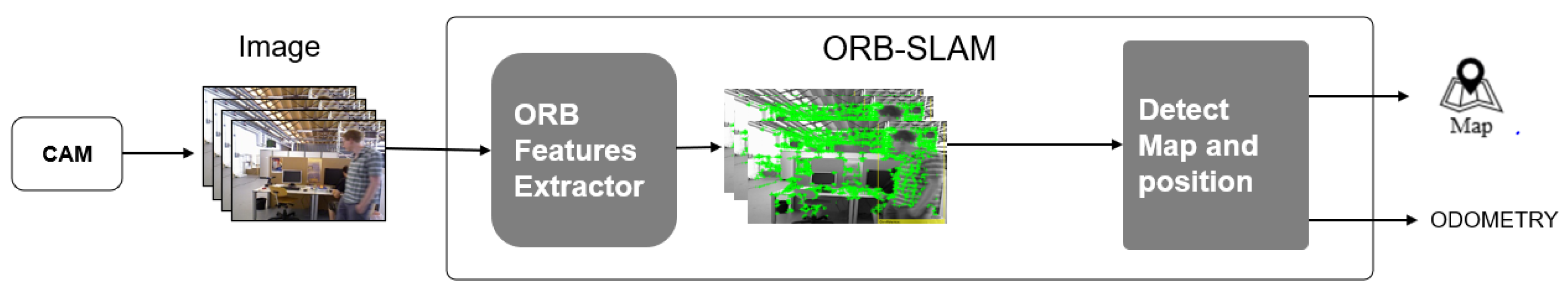
Figure 3.
ORB-SLAM.
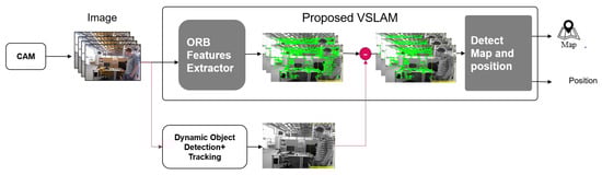
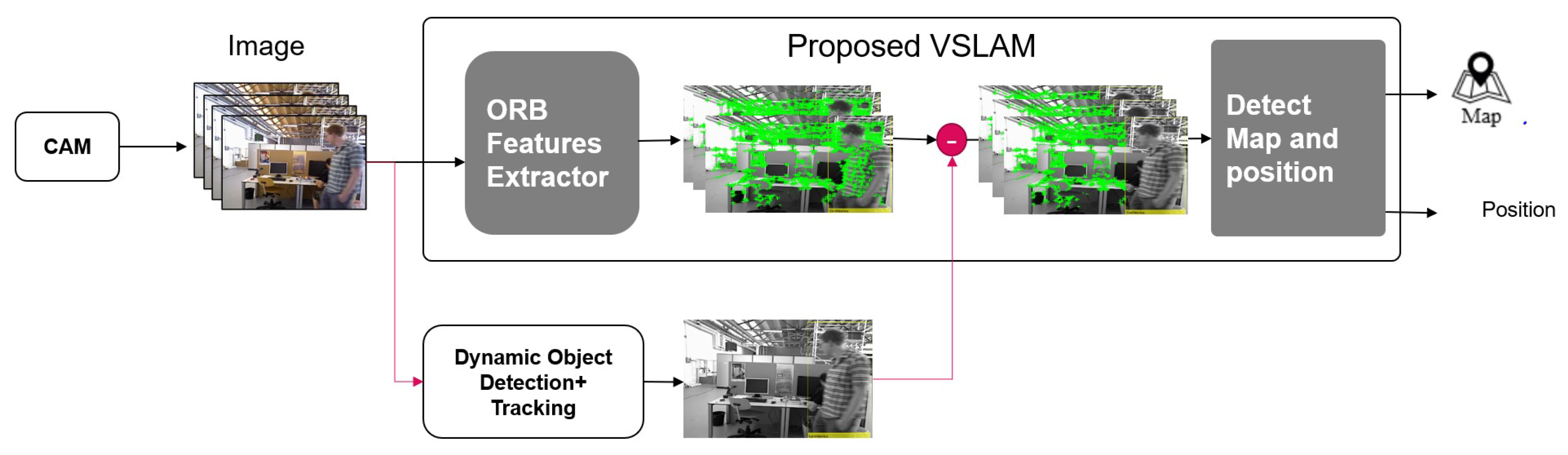
Figure 4.
Proposed SLAM.
VSLAM is a technique that processes input from a singular camera to deliver outputs as a 3D map and an estimate of the camera’s position, as depicted in Figure 2. The estimated position of the camera is essential for navigation purposes, and the 3D map plays a key role in comprehending the camera’s surroundings and identifying obstacles.
ORB-SLAM, as a VSLAM technique, employs the ORB (Oriented FAST and Rotated BRIEF) feature detector to identify keypoints within a camera’s imagery, as illustrated in Figure 3. ORB keypoints are pinpointed at unique image locations, including corners, edges, and blobs. The result of ORB-SLAM is an environmental map alongside the estimated location and orientation of the camera. This map is constructed from tracked keypoints and their corresponding descriptors, which are refined through bundle adjustment. An estimation of the camera’s position and orientation is derived from this map in conjunction with the camera’s movements.
In this research, ORB-SLAM is integrated with the method of detecting and tracking (as illustrated in Figure 4) to address the challenge of localization drift induced by dynamic objects. The YOLOv4 algorithm is applied alongside Kalman tracking modules for each keyframe identified by ORB-SLAM. Whenever dynamic objects are detected, a matrix operation is executed to remove the keypoints situated within the bounding boxes of these objects. This approach significantly improves localization accuracy by excluding the drift caused by keypoints associated with dynamic objects while concurrently endeavoring to preserve the fidelity of the environmental map.
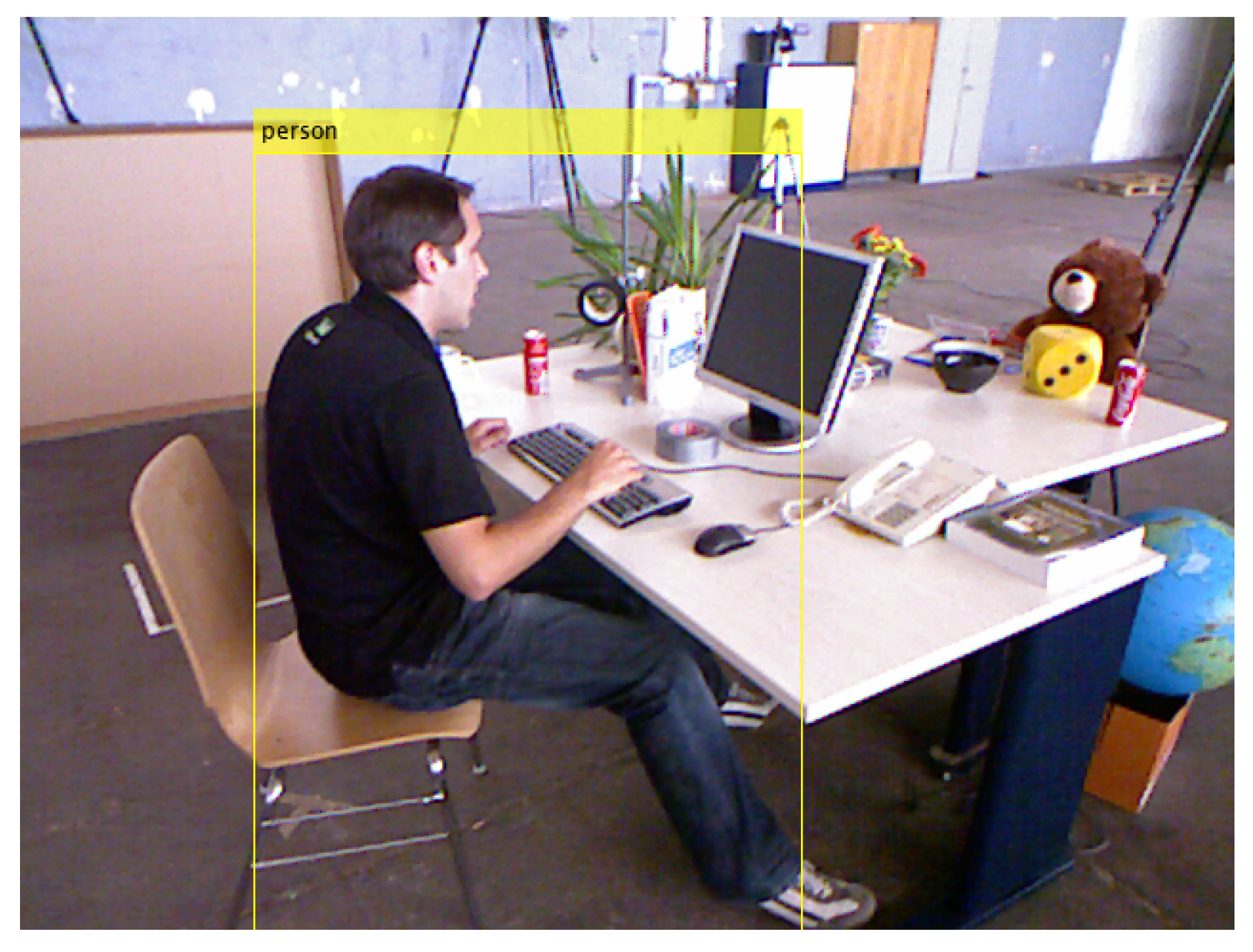
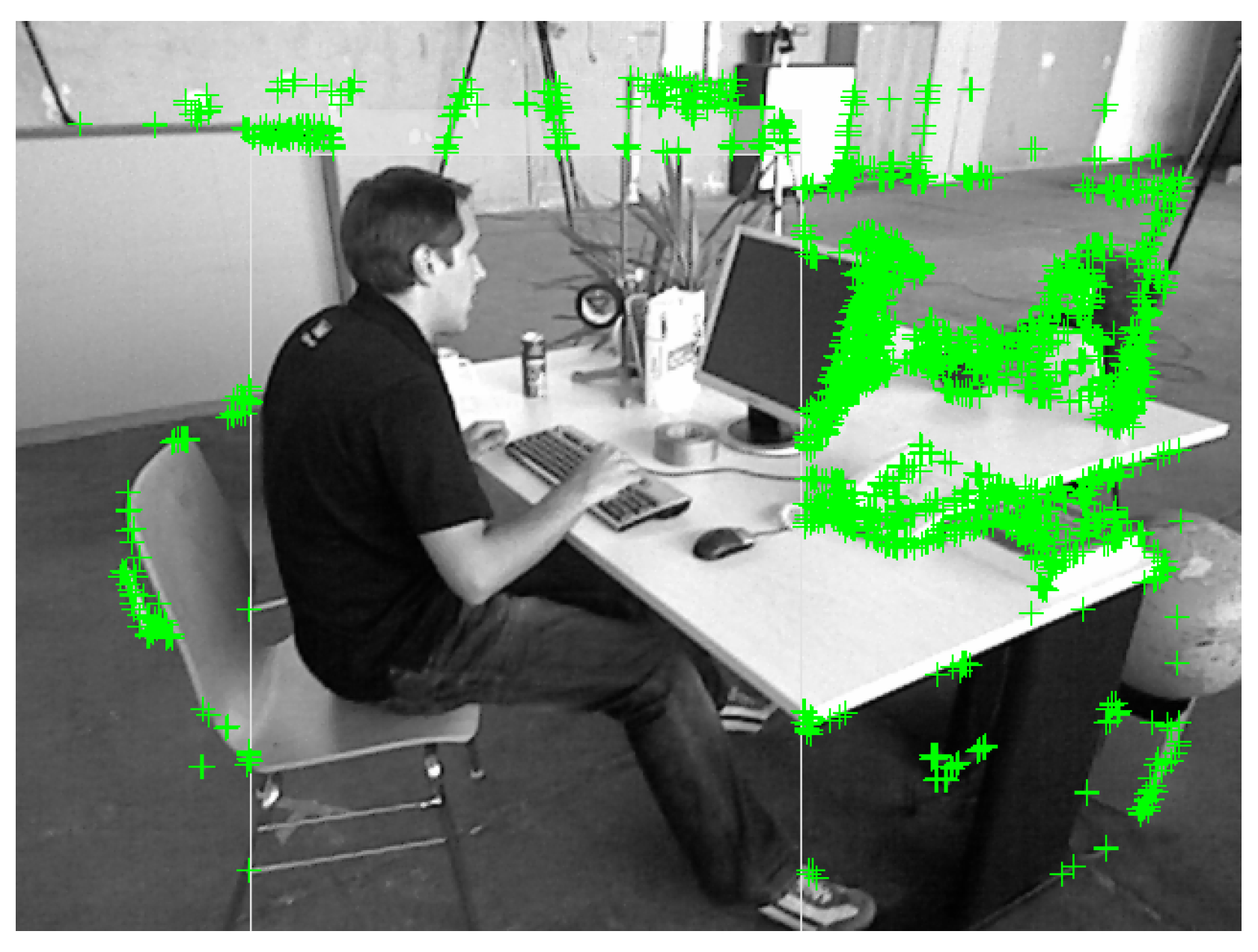
Thanks to the capabilities of YOLOv4, as illustrated in Figure 5, a dynamic entity such as a person is accurately identified. Following the detection of dynamic objects and their bounding boxes, a movement model of the boxes is integrated with the Kalman filter to track all identified objects. This strategy is known as the multi-object tracking method, and further details can be found in [36]. Subsequently, this detection and tracking process is combined with ORB features to pinpoint features within the predicted boxes, as depicted in Figure 6. In the final step, algorithms are implemented to remove the keypoints associated with unwanted dynamic objects, a process showcased in Figure 7.

Figure 5.
Outcomes of dynamic object detection using YOLOv4 (adapted from [37]).
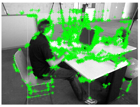
Figure 6.
Outcomes of ORB feature function (adapted from [37]).

Figure 7.
Results of dynamic feature point (adapted from [37]).
Integrating visual SLAM with the YOLO-Kalman module offers an effective strategy for rectifying inaccuracies introduced by dynamic objects within a real-world setting. In this methodology, the integration of ORB-SLAM and the YOLO-Kalman framework delivers precise and dependable assessments of the camera’s location and alignment alongside environmental mapping, even in the presence of dynamic entities. By merging the outcomes of YOLOv4 object detection with the visual SLAM framework, this approach can avoid any discrepancies resulting from moving objects.
In the study, the TUM public datasets were utilized for analysis [37]. Figure 5, Figure 6 and Figure 7 were derived from this dataset. Modifications to the original data included object detection using YOLOv4, outcomes of the ORB feature, and the results of dynamic features. These alterations were made to highlight image features relevant to the research objectives.
3.5. Typical Kalman Filter
A widely adopted method for estimating parameters involves deploying an observer that relies on a state space model. Such an estimator is capable of inferring unobservable states within a system, as detailed in the referenced paper on state estimation [38]. By leveraging the known input and output signals of a system, it is possible to estimate its internal states. The main goal is to use an estimator to either monitor states that cannot be directly measured or to minimize uncertainties associated with real-world sensor data. Nonetheless, the precision of these estimations hinges critically on the accuracy of the underlying model.
Initially, consider a tracking system in which the state vector represents the dynamic characteristics of the object, with k signifying the temporal aspect of the discretized object box model. In this context, the aim is to deduce based on observed measurements .
Consider the following equation that represents the model of the internal state:
In this context, F represents the transition matrix, while denotes the state transitioning from time to k.
is a Gaussian distribution of a random variable characterized by an average and a covariance. With a normal probability distribution, is as follows:
The state of measurement from time to k is defined as follows:
Here, H denotes the measurement matrix, and is the Gaussian distribution of a random variable is characterized by an average and a covariance. With a normal probability distribution, is as follows:
The estimation process is divided into two phases: the time-update equations and the measurement-update equations. The notation signifies the state at time k based on the data available up to time . The time-update equations are responsible for predicting the estimated states () and the estimated error covariance () for the upcoming time step. The overall algorithm is described as follows:
The measurement-update equations serve to adjust the predicted estimated states and error covariance from the time-update phase by comparing the estimated states against actual measurements. These equations are outlined as follows:
Here, and are positive definite matrices representing the covariances of process noise and measurement noise, respectively. It is important to note that the process noise and measurement noise in Kalman filters are assumed to be white Gaussian noise and are independent from each other. This independence is a crucial prerequisite for the estimator’s convergence.
3.6. Object Tracking Using Kalman Filter
For the purpose of identifying and monitoring moving objects recorded by a camera, it is essential to examine their features, such as their positions, geometries, and centroids [39]. The camera employed in this research captures images at a rate of 30 frames per second (30 fps), resulting in minimal changes between two consecutive frames for moving objects. This allows us to consider the movement of the target object to be scontinuous over adjacent frames.
To effectively describe a moving object, focus is placed on its centroid position and the tracking window size. By using these features, a representation that accurately describes the object’s motion can be created. Once moving objects have been identified through learning methods, certain preparatory steps are required for tracking these objects.
A key step involves allocating a tracking window to every moving object within a scene. To minimize the impact of excessive noise, the tracking window size is maintained at a modest scale set slightly larger than the object’s image. This approach aids in diminishing noise disturbances, improving image processing efficiency, and increasing the speed of operation.
The Kalman filter applied in tracking is characterized by its states, the motion model, and the equation matrix of measurements. The system state vector is eight-dimensional and can be represented as follows:
Here, and denote the horizontal and vertical coordinates of the centroid, while and indicate the half-width and half-height of the tracking window, respectively. , , , and represent the respective velocities of these parameters.
The measurement vector of the system adopts the following:
In what follows, F represents the transition matrix and H denotes the measurement matrix of our tracking system, accompanied by the Gaussian process and the measurement noise . The magnitudes of these noise values rely entirely on the characteristics of the system under observation and are determined through empirical adjustments.
The observation matrix H can be defined as follows:
Once the state and measurement equations of the motion model have been established, the Kalman filter can be applied in the subsequent frame to predict the position and dimensions of the object within a limited area, thereby obtaining the trajectories of moving objects.
4. Results and Discussion
In this section, the outcomes from both the standard ORB-SLAM and the enhanced ORB-SLAM integrated with YOLO methods are presented, and these results are compared against those obtained from the proposed approach that combines ORB-SLAM and YOLO-Kalman. For more detailed information regarding ORB-SLAM combined with YOLO, please refer to previous work [40]. First, the results of the ORB-SLAM method in comparison to the ORB-SLAM with YOLO-Kalman method are showcased, focusing on the 3D and xyz axes. Second, a comparison of 2D trajectory results for both algorithms, ORB-SLAM and ORB-SLAM with YOLO-Kalman, is provided. Finally, a table summarizing the results for the ORB alone, ORB-SLAM with YOLO, and the proposed ORB-SLAM with YOLO-Kalman methods is included.
TUM (Technical University of Munich) datasets designed for RGB-D SLAM systems were utilized for algorithm assessment, as referenced in [37]. This database is extensively employed in SLAM research and evaluation due to its provision of high-quality data accompanied by ground-truth poses crucial for appraising VSLAM algorithms. Essentially, the TUM datasets encompass a variety of environments and scenarios, such as dynamic environments, object SLAM, and suboptimal lighting conditions. With its collection of indoor and outdoor scenes, both dynamic and static objects, and diverse lighting conditions, the TUM database serves as a valuable tool for examining the performance of SLAM algorithms across a range of situations. Finally, the TUM datasets are primarily utilized within academic and research circles, facilitating the comparison of various SLAM algorithms’ performances. They are also employed for assessing ORB-SLAM in Matlab, which aligns with our objective of evaluating our work. While numerous databases like KITTI [41] and EuRoC [42] are available for SLAM algorithm evaluation in research, the TUM datasets are especially favored for their capability to assess SLAM performance in dynamic environments. This preference is due to the datasets’ inclusion of sequences with substantial dynamic object interactions in addition to their accuracy and broad adoption in the research community.
Moreover, the choice to use the Matlab environment is driven by its high-level programming language and interactive framework, which facilitate the rapid prototyping, comparison, and visualization of complex algorithms and data. Matlab offers an interactive suite of tools and functionalities tailored for the robotics community, including several specialized toolboxes like the Robotics System Toolbox and Mapping Toolbox. These toolboxes are equipped with functions designed for managing robot sensors, kinematics, and mapping tasks. This comprehensive toolset renders Matlab an ideal platform for devising innovative approaches to addressing the complexities of VSLAM [43].
The evaluation primarily focused on the key feature of the ORB-SLAM and YOLO-Kalman system, namely the removal of dynamic objects to correct trajectory drift, utilizing real-time experiments on the public TUM dataset. It should be noted that map accuracy was not assessed in this study. For the datasets, the TUM freiburg2-desk-with-person sequence was selected, depicting a typical office setting with an individual sitting and moving throughout the recording.
This particular sequence is well-suited for assessing the effectiveness of our ORB-SLAM with YOLO-Kalman system in managing dynamic object removal and model correction. The video sequence lasts for 142.08 s, during which the camera covers a distance of 17.044 m, moving at an average velocity of 0.121 m per second.
The methodology for computing the improvement criterion in terms of the RMSE is depicted in Equation (14):
The method for calculating the RMSE is provided in Equation (15):
where represents the set of points predicted by the ORB-SLAM algorithm, and denotes the set of points predicted by the ORB-SLAM with YOLO-Kalman enhancement.
The calculation method for the RMSE in the 3D position is given in Equation (16):
In conclusion, this paper defines the deviation error as the maximum amplitude of the absolute error.
Initially, the proposed method was evaluated against the original ORB-SLAM method, demonstrating enhanced performance in accurately estimating the camera trajectory, even in highly dynamic settings. In the subsequent results, the term “without YOLO-Kalman” refers to the outcomes derived solely from the original ORB-SLAM.
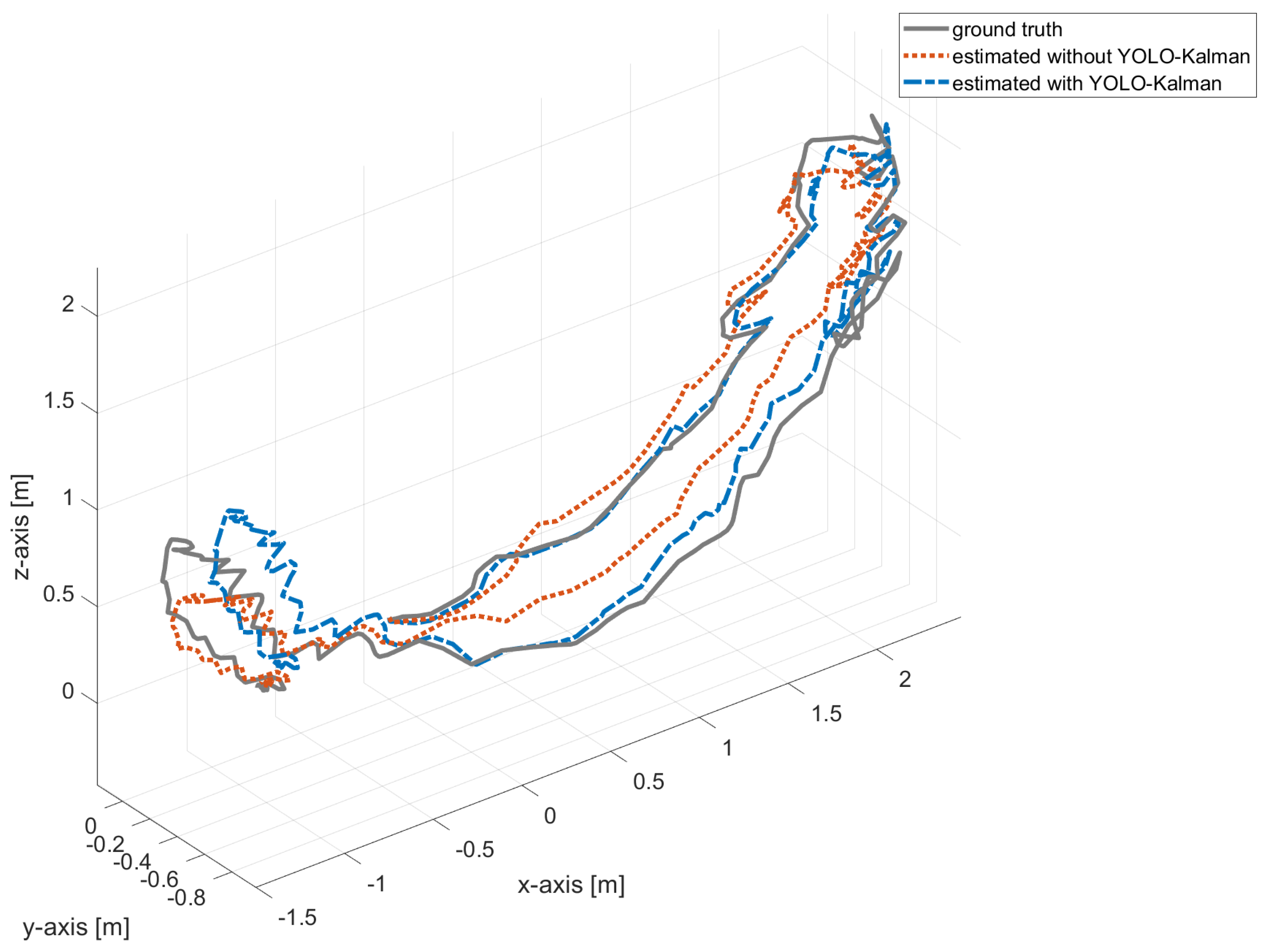
Figure 8 depicts three distinct trajectories: the initial one represents the ground-truth trajectory, the second is generated by ORB-SLAM, and the third shows the outcome of implementing ORB-SLAM with the YOLO-Kalman algorithm. The recording appears to have occurred within a 4-m range on the x-axis, a 1-m range on the y-axis, and a 2-m range on the z-axis, all while rotating on a desktop table. Further analyses of the impact of dynamic object removal on ORB-SLAM’s performance will be presented for each axis in the subsequent results.
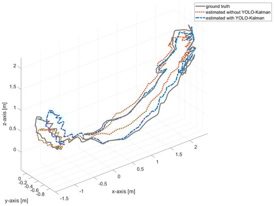
Figure 8.
Three-dimensional trajectory outcomes: ORB-SLAM and enhanced ORB-SLAM with YOLO-Kalman on the freiburg2-desk-with-person dataset.
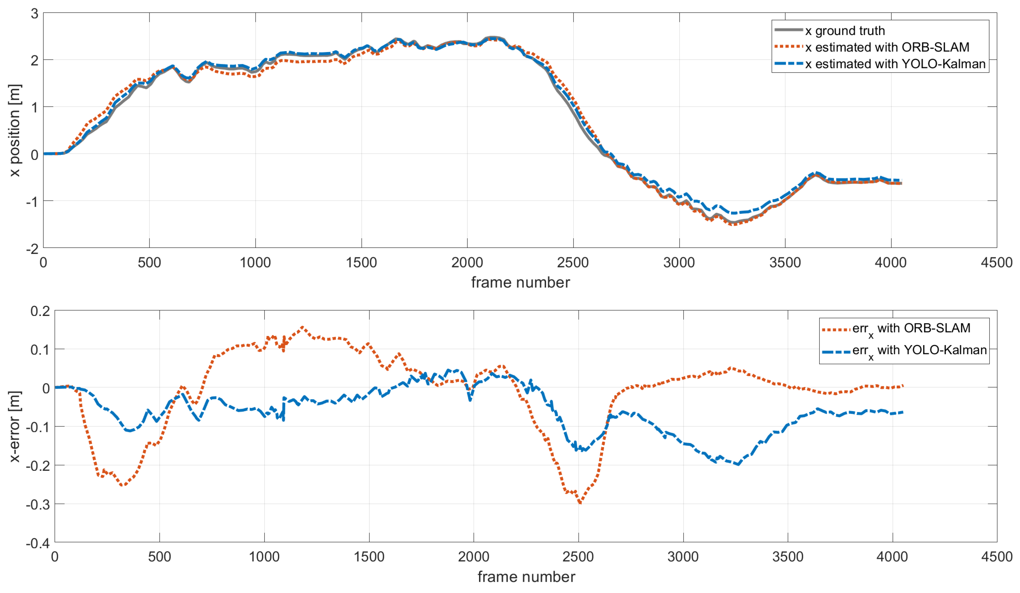
The data presented in Figure 9 illustrate the estimated positions and their corresponding errors along the x-axis. From an analysis of the errors, a significant enhancement is observed. The deviation error for the ORB-SLAM algorithm tops out at just over 30.18 cm, while the ORB-SLAM algorithm integrated with YOLO-Kalman demonstrates a lower maximum deviation error of 19.03 cm, showcasing an improvement compared to the original ORB-SLAM.
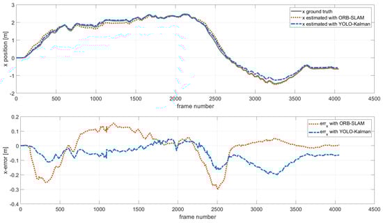
Figure 9.
Estimated positions and errors of ORB-SLAM and ORB-SLAM with YOLO-Kalman applied on the x-axes.
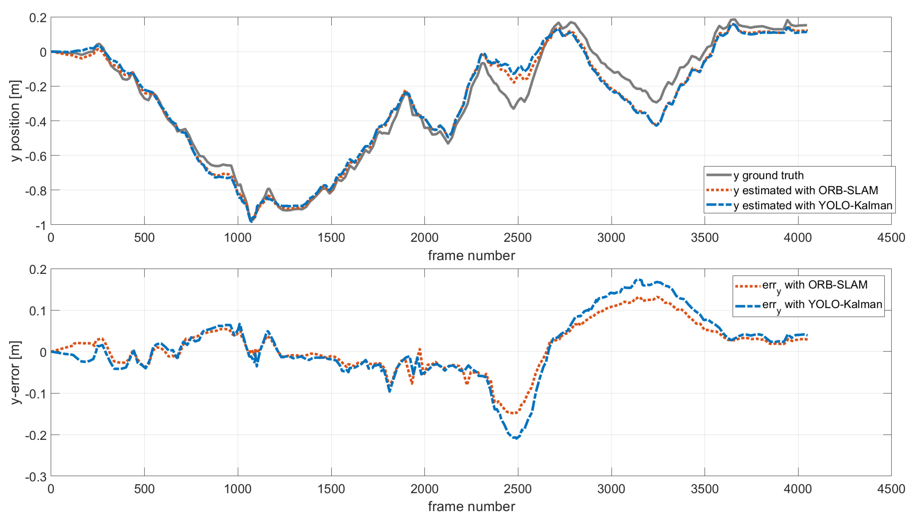
Figure 10 presents the outcomes of the experiment focused on estimating positions and errors along the y-axis. The results highlight a limitation in the ORB-SLAM with YOLO-Kalman method’s precision in estimating the y-axis position. Nonetheless, the overall conclusion demonstrates that despite this shortcoming, the integration of ORB-SLAM with YOLO-Kalman results in a method that surpasses the performance of the original ORB-SLAM in predicting 3D trajectories.
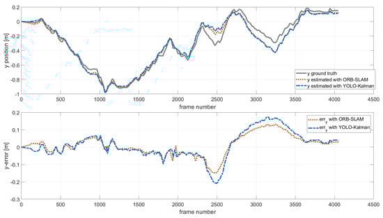
Figure 10.
Estimated positions and errors of ORB-SLAM and ORB-SLAM with YOLO-Kalman applied on the y-axes.
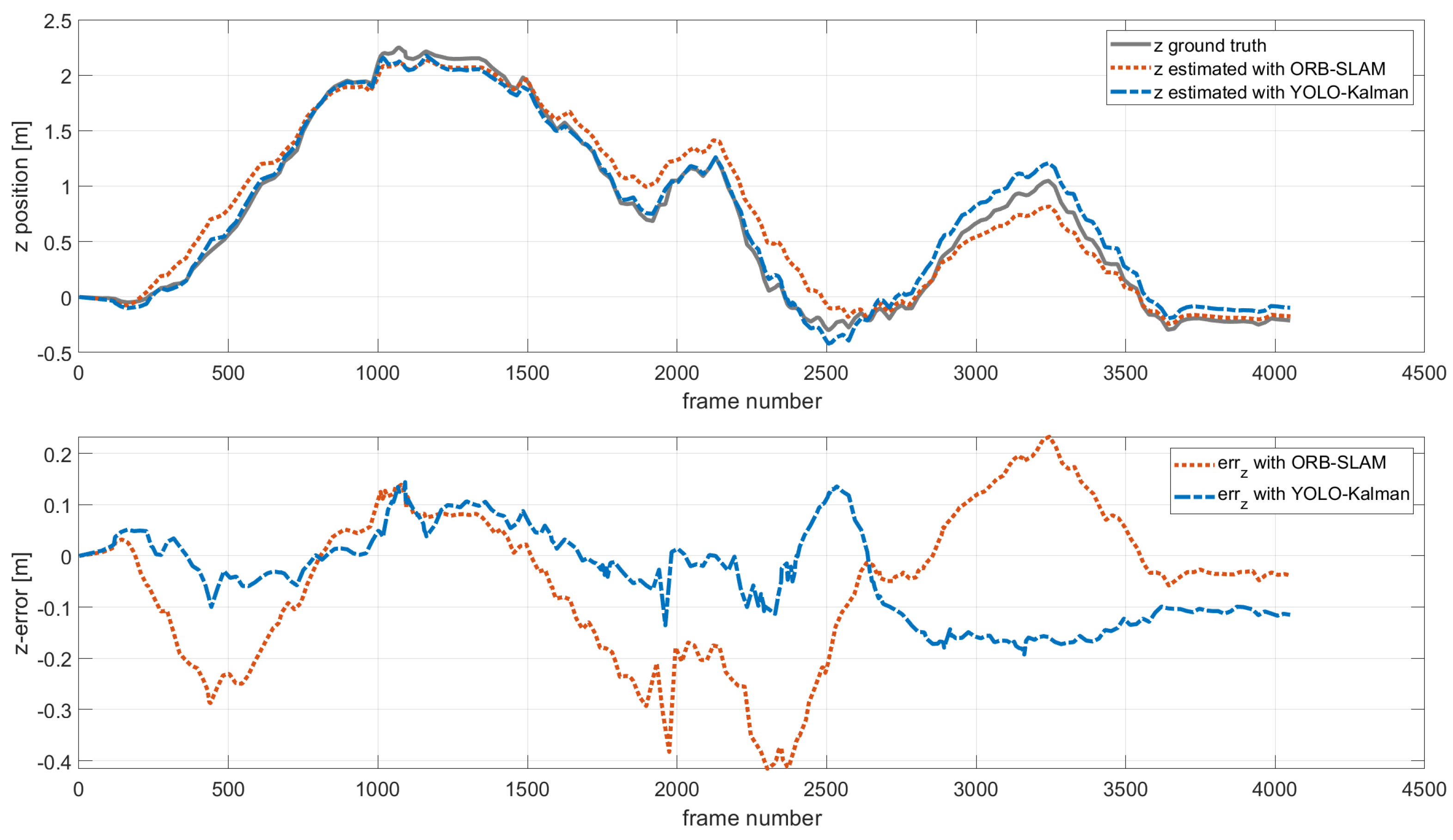
Figure 11 displays the z-axis trajectory outcomes from our proposed VSLAM algorithm in comparison with those from ORB-SLAM. The trajectory generated by our method appears to closely match the actual camera trajectory. Regarding deviation error, the ORB-SLAM algorithm’s maximum reaches just over 41.57 cm. In contrast, the ORB-SLAM integrated with YOLO-Kalman shows a significantly lower maximum of 20.20 cm, indicating an improvement over the original ORB-SLAM. This demonstrates that the error in trajectory prediction by the proposed approach is considerably smaller compared to ORB-SLAM, underscoring the superior quality of the trajectory prediction results achieved by our proposed method.
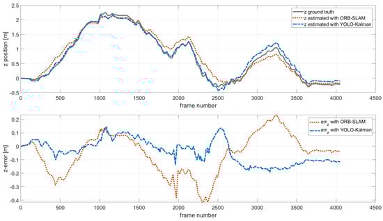
Figure 11.
Estimated positions and errors of ORB-SLAM and ORB-SLAM with YOLO-Kalman applied on the z-axes.
Additionally, the keyframe count gives 273 with the YOLO-Kalman method; a keyframe count of 254 shows the augmented number of keyframes found when using YOLO-Kalman algorithms.
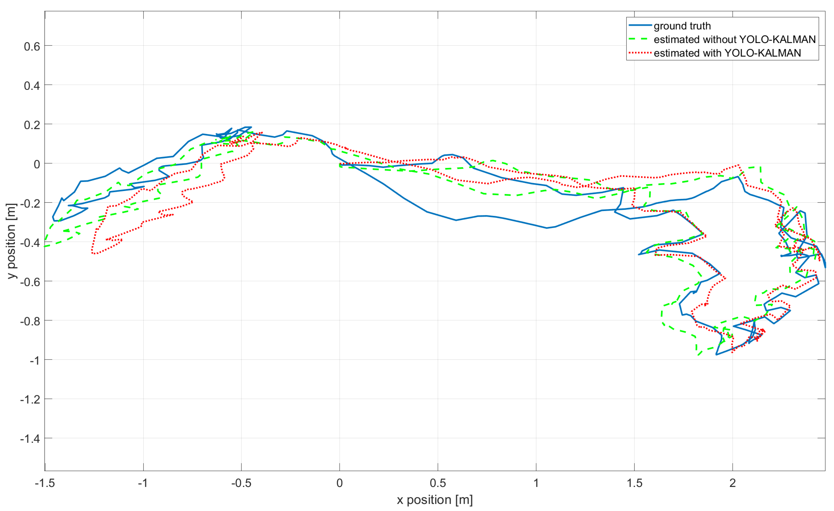
Figure 12 displays 2D plots from the ORB-SLAM method and the proposed methodology with YOLO-Kalman for the dataset “freiburg2-desk-with-person”. It can be observed that the estimated trajectory obtained with the proposed method closely aligns with the real trajectory compared to ORB-SLAM when moving along the y-axis in the right-hand section, where x is greater than 1.5 m. However, a limitation becomes evident in the left-hand section when x is less than 0.5, especially when traversing along both the x- and y-axes.
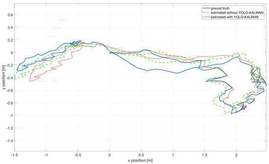
Figure 12.
Two-dimensional trajectory outcomes: ORB-SLAM and enhanced ORB-SLAM with YOLO-Kalman on the freiburg2-desk-with-person dataset.
After presenting the estimation results figures for the ORB-SLAM and ORB-SLAM with YOLO-Kalman methods, the outcomes of ORB-SLAM integrated with YOLO are included in the table below for a comprehensive comparison with the method employing YOLO-Kalman.
The integration of ORB-SLAM with YOLO, as explained in previous work, is a technique used to enhance VSLAM by eliminating features on dynamic objects, using only YOLOv4 for object detection. However, this technique suffers from discontinuities in object detection.
Table 1 presents the trajectory results of the proposed method integrating ORB-SLAM the YOLO-Kalman algorithm compared against the results from the original ORB-SLAM and ORB-SLAM enhanced with YOLO methods. In this table, the improvement criterion is presented in relation to ORB-SLAM. ORB-SLAM with only object detection shows an improvement of 23.85% compared to 34.99% when using tracking methods. This highlights the importance of addressing the weakness of ORB-SLAM with only YOLO, which comprises in detecting objects that arise from relying solely on detection. The improvement criterion in ORB-SLAM with YOLO-Kalman validates the choice of the YOLO-Kalman corrector.

Table 1.
Comparative results: proposed ORB-SLAM with YOLO-Kalman method vs. original ORB-SLAM and ORB-SLAM with YOLO methods.
The proposed algorithm outperforms others primarily because it operates within the SLAM framework, where the camera-tracking step relies on features extracted by the ORB algorithm. This algorithm does not differentiate between dynamic and static objects, assuming the entire scene is static. This leads to the execution of the “local map tracking” algorithm based on potentially inaccurate feature measurements from a mistakenly assumed static scene despite the presence of dynamic objects, which makes the environment dynamic. An incorrect tracking estimation influenced by dynamic objects can result. To address this, the algorithm is designed to detect and track objects in real time, effectively eliminating features associated with dynamic objects and reducing the uncertainty these objects introduce in the camera-tracking phase.
Furthermore, considering all the results discussed in this article, which demonstrate the enhancement of the ORB-SLAM algorithm for drone localization in a dynamic environment, it is noteworthy that there is a loss of precision along the y-axis. This underscores the neeed for further investigation to refine the results and explore the feasibility of integrating the algorithm for dynamic object elimination with other SLAM algorithms. Future work could also benefit from considering advanced detection techniques, such as object elimination and inpainting methods, to further enhance accuracy.
5. Conclusions
This paper addresses the challenge of dynamic objects in visual simultaneous localization and mapping (SLAM). To tackle this challenge, the Kalman filter was incorporated to track multiple dynamic objects, assisting the YOLOv4 detector in handling object discontinuities and optimizing keyframe deletion. These efforts significantly enhanced monocular SLAM performance, utilizing a cost-effective vision sensor and reducing the influence of dynamic objects in real-time settings.
Future research could explore the feasibility of integrating this dynamic object elimination algorithm with other SLAM algorithms. Additionally, considering advanced detection techniques, such as object elimination and inpainting methods, could further improve the overall system.
The proposed detection and tracking model shows great potential for future applications, particularly in UAV-based surveillance. Implementing this model in real-world scenarios can enhance UAV systems’ navigation accuracy and their ability to detect and track suspicious objects. This integrated approach not only ensures precise position estimation for UAVs but also provides a valuable module for continuous surveillance missions.
Author Contributions
Conceptualization, Y.E.G.; methodology, Y.E.G.; software, Y.E.G. and M.M.; validation, Y.E.G., F.K. and M.M.; formal analysis, Y.E.G.; investigation, Y.E.G.; resources, Y.E.G.; data curation, Y.E.G.; writing—original draft preparation, Y.E.G., F.K. and M.M.; writing—review and editing, Y.E.G., F.K., M.M. and C.L.; supervision, F.K., M.M. and C.L.; project administration, F.K., M.M. and C.L. All authors have read and agreed to the published version of the manuscript.
Funding
This research received no external funding.
Informed Consent Statement
Not applicable.
Data Availability Statement
The dataset utilized in this study is the publicly available TUM dataset. Here is a link: https://vision.in.tum.de/data/datasets/rgbd-dataset (accessed on 27 March 2024).
Conflicts of Interest
The authors declare no conflicts of interest.
Abbreviations
The following abbreviations are used in this manuscript:
| UAV | unmanned aerial vehicle |
| IMU | inertial measurement unit |
| LiDAR | laser imaging, detection, and ranging |
| SLAM | simultaneous localization and mapping |
| MTT | multi-target tracking |
| EKF | extended Kalman filter |
| SSD | single-shot multibox detector |
| RMSE | root-mean-square error |
| YOLO | You Only Look Once |
| ORB | oriented fAST and rotated brief |
| GNSS | global navigation satellite system |
References
- Rejeb, A.; Abdollahi, A.; Rejeb, K.; Treiblmaier, H. Drones in agriculture: A review and bibliometric analysis. Comput. Electron. Agric. 2022, 198, 107017. [Google Scholar] [CrossRef]
- Erdos, D.; Erdos, A.; Watkins, S.E. An experimental UAV system for search and rescue challenge. IEEE Aerosp. Electron. Syst. Mag. 2013, 28, 32–37. [Google Scholar] [CrossRef]
- Utsav, A.; Abhishek, A.; Suraj, P.; Badhai, R.K. An IoT based UAV network for military applications. In Proceedings of the 2021 Sixth International Conference on Wireless Communications, Signal Processing and Networking (WiSPNET), Chennai, India, 25–27 March 2021; pp. 122–125. [Google Scholar]
- Haq, M.A.; Rahaman, G.; Baral, P.; Ghosh, A. Deep learning based supervised image classification using UAV images for forest areas classification. J. Indian Soc. Remote Sens. 2021, 49, 601–606. [Google Scholar] [CrossRef]
- Gong, J.; Chang, T.H.; Shen, C.; Chen, X. Flight time minimization of UAV for data collection over wireless sensor networks. IEEE J. Sel. Areas Commun. 2018, 36, 1942–1954. [Google Scholar] [CrossRef]
- Mohamed, N.; Al-Jaroodi, J.; Jawhar, I.; Idries, A.; Mohammed, F. Unmanned aerial vehicles applications in future smart cities. Technol. Forecast. Soc. Chang. 2020, 153, 119293. [Google Scholar] [CrossRef]
- Available online: https://www.azurdrones.com/fr/ (accessed on 1 December 2023).
- Available online: https://sunflower-labs.com/ (accessed on 1 December 2023).
- Gupta, A.; Afrin, T.; Scully, E.; Yodo, N. Advances of UAVs toward Future Transportation: The State-of-the-Art, Challenges, and Opportunities. Future Transp. 2021, 1, 326–350. [Google Scholar] [CrossRef]
- Mur-Artal, R.; Tardós, J.D. Orb-slam2: An open-source slam system for monocular, stereo, and RGB-D cameras. IEEE Trans. Robot. 2017, 33, 1255–1262. [Google Scholar] [CrossRef]
- López, E.; García, S.; Barea, R.; Bergasa, L.M.; Molinos, E.J.; Arroyo, R.; Romera, E.; Pardo, S. A Multi-Sensorial Simultaneous Localization and Mapping (SLAM) System for Low-Cost Micro Aerial Vehicles in GPS-Denied Environments. Sensors 2017, 17, 802. [Google Scholar] [CrossRef]
- Ćwian, K.; Nowicki, M.R.; Skrzypczyński, P. GNSS-augmented lidar slam for accurate vehicle localization in large scale urban environments. In Proceedings of the 2022 17th International Conference on Control, Automation, Robotics and Vision (ICARCV), Singapore, 11–13 December 2022; pp. 701–708. [Google Scholar]
- Qian, J.; Chen, K.; Chen, Q.; Yang, Y.; Zhang, J.; Chen, S. Robust visual-lidar simultaneous localization and mapping system for UAV. IEEE Geosci. Remote Sens. Lett. 2021, 19, 1–5. [Google Scholar] [CrossRef]
- Haq, M.A. CNN based automated weed detection system using UAV imagery. Comput. Syst. Sci. Eng. 2022, 42, 837–849. [Google Scholar]
- Singandhupe, A.; La, H.M. A review of slam techniques and security in autonomous driving. In Proceedings of the 2019 Third IEEE International Conference on Robotic Computing (IRC), Naples, Italy, 25–27 February 2019; pp. 602–607. [Google Scholar]
- Shan, Z.; Li, R.; Schwertfeger, S. RGBD-Inertial Trajectory Estimation and Mapping for Ground Robots. Sensors 2019, 19, 2251. [Google Scholar] [CrossRef] [PubMed]
- Available online: https://www.ecologie.gouv.fr/ (accessed on 1 December 2023).
- Sachdev, K.; Gupta, M.K. A comprehensive review of feature based methods for drug target interaction prediction. J. Biomed. Inform. 2019, 93, 103159. [Google Scholar] [CrossRef] [PubMed]
- Cremers, D. Direct methods for 3d reconstruction and visual slam. In Proceedings of the 2017 Fifteenth IAPR International Conference on Machine Vision Applications (MVA), Nagoya, Japan, 8–12 May 2017; pp. 34–38. [Google Scholar]
- Engel, J.; Schöps, T.; Cremers, D. LSD-SLAM: Large-scale direct monocular SLAM. In Proceedings of the European Conference on Computer Vision, Zurich, Switzerland, 6–12 September 2014; Springer International Publishing: Cham, Switzerland, 2014; pp. 834–849. [Google Scholar]
- Silveira, G.; Malis, E.; Rives, P. An efficient direct approach to visual SLAM. IEEE Trans. Robot. 2008, 24, 969–979. [Google Scholar] [CrossRef]
- Basiri, A.; Mariani, V.; Glielmo, L. Improving Visual SLAM by Combining SVO and ORB-SLAM2 with a Complementary Filter to Enhance Indoor Mini-Drone Localization under Varying Conditions. Drones 2023, 7, 404. [Google Scholar] [CrossRef]
- Kulchandani, J.S.; Dangarwala, K.J. Moving object detection: Review of recent research trends. In Proceedings of the 2015 International Conference on Pervasive Computing (ICPC), Pune, India, 8–10 January 2015; pp. 1–5. [Google Scholar]
- Ballester, I.; Fontán, A.; Civera, J.; Strobl, K.H.; Triebel, R. DOT: Dynamic object tracking for visual SLAM. In Proceedings of the 2021 IEEE International Conference on Robotics and Automation (ICRA), Xi’an, China, 30 May–5 June 2021; pp. 11705–11711. [Google Scholar]
- Zhang, X.; Zhang, R.; Wang, X. Visual SLAM Mapping Based on YOLOv5 in Dynamic Scenes. Appl. Sci. 2022, 12, 11548. [Google Scholar] [CrossRef]
- Bahraini, M.S.; Rad, A.B.; Bozorg, M. SLAM in Dynamic Environments: A Deep Learning Approach for Moving Object Tracking Using ML-RANSAC Algorithm. Sensors 2019, 19, 3699. [Google Scholar] [CrossRef] [PubMed]
- Bescos, B.; Fácil, J.M.; Civera, J.; Neira, J. DynaSLAM: Tracking, mapping, and inpainting in dynamic scenes. IEEE Robot. Autom. Lett. 2018, 3, 4076–4083. [Google Scholar] [CrossRef]
- Wu, X.; Huang, F.; Wang, Y.; Jiang, H. A VINS Combined With Dynamic Object Detection for Autonomous Driving Vehicles. IEEE Access 2022, 10, 91127–91136. [Google Scholar] [CrossRef]
- Yin, H.; Li, S.; Tao, Y.; Guo, J.; Huang, B. Dynam-SLAM: An Accurate, Robust Stereo Visual-Inertial SLAM Method in Dynamic Environments. IEEE Trans. Robot. 2022, 39, 289–308. [Google Scholar] [CrossRef]
- Zhong, F.; Wang, S.; Zhang, Z.; Wang, Y. Detect-SLAM: Making object detection and SLAM mutually beneficial. In Proceedings of the 2018 IEEE Winter Conference on Applications of Computer Vision (WACV), Lake Tahoe, NV, USA, 12–15 March 2018. [Google Scholar]
- Wang, E.; Zhou, Y.; Zhang, Q. Improved Visual Odometry Based on SSD Algorithm in Dynamic Environment. In Proceedings of the 2020 39th Chinese Control Conference (CCC), Shenyang, China, 27–29 July 2020. [Google Scholar]
- Lu, X.; Wang, H.; Tang, S.; Huang, H.; Li, C. DM-SLAM: Monocular SLAM in Dynamic Environments. Appl. Sci. 2020, 10, 4252. [Google Scholar] [CrossRef]
- Chen, W.; Shang, G.; Ji, A.; Zhou, C.; Wang, X.; Xu, C.; Li, Z.; Hu, K. An Overview on Visual SLAM: From Tradition to Semantic. Remote Sens. 2022, 14, 3010. [Google Scholar] [CrossRef]
- Mur-Artal, R.; Montiel, J.M.M.; Tardos, J.D. ORB-SLAM: A versatile and accurate monocular SLAM system. IEEE Trans. Robot. 2015, 31, 1147–1163. [Google Scholar] [CrossRef]
- Bochkovskiy, A.; Wang, C.Y.; Liao, H.Y.M. Yolov4: Optimal speed and accuracy of object detection. arXiv 2020, arXiv:2004.10934. [Google Scholar]
- Li, X.; Wang, K.; Wang, W.; Li, Y. A multiple object tracking method using Kalman filter. In Proceedings of the 2010 IEEE International Conference on Information and Automation, Harbin, China, 20–23 June 2010; pp. 1862–1866. [Google Scholar]
- Sturm, J.; Engelhard, N.; Endres, F.; Burgard, W.; Cremers, D. A benchmark for the evaluation of RGB-D SLAM systems. In Proceedings of the 2012 IEEE/RSJ International Conference on Intelligent Robots and Systems, Vilamoura-Algarve, Portugal, 7–12 October 2012; pp. 573–580. [Google Scholar]
- Simon, D. Kalman filtering. Embed. Syst. Program. 2001, 14, 72–79. [Google Scholar]
- Weng, S.K.; Kuo, C.M.; Tu, S.K. Video object tracking using adaptive Kalman filter. J. Vis. Commun. Image Represent. 2006, 17, 1190–1208. [Google Scholar] [CrossRef]
- El Gaouti, Y.; Khenfri, F.; Mcharek, M.; Larouci, C. Using object detection for a robust monocular SLAM in dynamic environments. In Proceedings of the 2023 IEEE 32nd International Symposium on Industrial Electronics (ISIE), Helsinki, Finland, 19–21 June 2023; pp. 1–6. [Google Scholar] [CrossRef]
- Geiger, A.; Lenz, P.; Urtasun, R. Are we ready for autonomous driving? the kitti vision benchmark suite. In Proceedings of the 2012 IEEE Conference on Computer Vision and Pattern Recognition, Providence, RI, USA, 16–21 June 2012. [Google Scholar]
- Burri, M.; Nikolic, J.; Gohl, P.; Schneider, T.; Rehder, J.; Omari, S.; Achtelik, M.W.; Siegwart, R. The EuRoC micro aerial vehicle datasets. Int. J. Robot. Res. 2016, 35, 1157–1163. [Google Scholar] [CrossRef]
- Available online: https://fr.mathworks.com/help/vision/ug/monocular-visual-simultaneous-localization-and-mapping.html (accessed on 1 December 2023).


Disclaimer/Publisher’s Note: The statements, opinions and data contained in all publications are solely those of the individual author(s) and contributor(s) and not of MDPI and/or the editor(s). MDPI and/or the editor(s) disclaim responsibility for any injury to people or property resulting from any ideas, methods, instructions or products referred to in the content. |
© 2024 by the authors. Licensee MDPI, Basel, Switzerland. This article is an open access article distributed under the terms and conditions of the Creative Commons Attribution (CC BY) license (https://creativecommons.org/licenses/by/4.0/).