A Composite Half-Normal-Pareto Distribution with Applications to Income and Expenditure Data

Abstract

The half-normal distribution is composited with the Pareto model to obtain a uni-parametric distribution with a heavy right tail, called the composite half-normal-Pareto distribution. This new distribution is useful for modeling positive data with atypical observations. We study the properties and the behavior of the right tail of this new distribution. We estimate the parameter using a method based on percentiles and the maximum likelihood method and assess the performance of the maximum likelihood estimator using Monte Carlo. We report three applications, one with simulated data and the others with income and expenditure data, in which the new distribution presents better performance than the Pareto distribution.

1. Introduction

Data of insurance claims, income, and other actuarial information present asymmetric behavior with heavy tails; these data are generally unimodal, with positive skewness and a heavy right tail. To model these data, therefore, investigators use heavy-tailed distributions, such as the Pareto distribution. The Pareto distribution has been widely used by many investigators, such as Beirlant et al. [1], Beirlant et al. [2] and Resnick [3].

A random variable X has a Pareto distribution (see Pareto [4]; Arnold [5]) with scale parameter $\theta$ and shape parameter $\alpha$ if its probability density function (pdf) is given by

$$f_X(x;\theta ,\alpha )=\frac{\alpha {\theta }^{\alpha }}{x^{1+\alpha }},x\ge \theta ,$$

with $\theta >0$ and $\alpha >0$.

The half-normal (HN) distribution is an important distribution for extending the normal distribution to the skew-normal distribution to flexibilize the asymmetry and the tails of the normal distribution (see Azzalini [6]; Henze [7]). We say that a random variable X has an HN distribution with a scale parameter $\sigma$ if its pdf is given by

$$f_X(x;\sigma )=\frac{2}{\sigma }\varphi \left(\frac{x}{\sigma }\right),x\ge 0,$$

with $\sigma >0$ and $\varphi (·)$ as the standard normal pdf. We denote this by $X\sim HN\left(\sigma \right)$. The respective cumulative distribution function (cdf) of X is

$$F_X(x;\sigma )=2\Phi \left(\frac{x}{\sigma }\right)-1,x\ge 0,$$

where $\Phi (·)$ is the cdf of the standard normal pdf. Furthermore, its quantile function (Q) is given by

$$Q\left(p\right)=\sigma {\Phi }^{-1}\left(\frac{1+p}{2}\right),0<p<1,$$

where ${\Phi }^{-1}$ is the inverse function of the cdf of the standard normal pdf.

The HN distribution has good properties, being a positive truncation of the normal distribution. Some extensions of the HN distribution are given by Cooray and Ananda [8] and Olmos et al. [9,10], among others.

The composite model methodology was introduced by Cooray and Ananda [11], who applied it to obtain the log-normal-Pareto model; Scollnik [12] discusses two extensions of the composite log-normal-Pareto model, while Cooray and Cheng [13] discuss the Bayesian estimators of the composite log-normal-Pareto model. Ciumara [14] obtained a composite Weibull–Pareto model, which they applied to actuarial data using the same design as Cooray and Ananda [11]. Cooray [15] reviewed the construction and properties of the composite Weibull–Pareto model, illustrating it in three sets of real data. Teodorescu [16] applied this methodology to a truncation of the log-normal Pareto model; Teodorescu and Panaitescu [17] applied it to a truncation of the Weibull–Pareto model, and Teodorescu and Vernic [18] applied it to the exponential-Pareto model; Scollnik and Sun [19] developed various composite Weibull–Pareto models and applied them to actuarial data; and Calderín-Ojeda et al. [20] studied the composite exponential arctan–Lognormal model and applied it to income data.

The composite distribution methodology is as follows:

$$f\left(x\right)=\left\{\begin{array}{cc}c{f}_1\left(x\right),\hfill & \mathrm{if}0<x\le \theta ,\hfill \\ \\ c{f}_2\left(x\right),\hfill & \mathrm{if}\theta \le x<\infty ,\hfill \end{array}\right.$$

(1)

where $f_1$ and $f_2$ are densities with positive support and c is the normalization constant. The following restrictions must also be met

• $f_1\left(\theta \right)=f_2\left(\theta \right)$
• ${\displaystyle \frac{d}{dx}}{f}_1{\left(x\right)|}_{x=\theta }={\displaystyle \frac{d}{dx}}{f}_2{\left(x\right)|}_{x=\theta }$

The composite exponential-Pareto (CEP) model studied by Teodorescu and Vernic [18] has only one parameter, and our proposal offers an alternative. We say that a random variable X has a CEP distribution with scale parameter $\theta$ if its pdf is given by

$$f(x;\theta )=\left\{\begin{array}{cc}\frac{0.775}{\theta }exp\left(-\frac{1.35x}{\theta }\right),\hfill & \mathrm{if}0<x\le \theta ,\hfill \\ \\ \frac{0.2{\theta }^{0.35}}{x^{1.35}},\hfill & \mathrm{if}\theta \le x<\infty .\hfill \end{array}\right.$$

(2)

The object of the present article is to introduce a composite distribution combining the HN and Pareto distributions. The new distribution obtained has a HN density up to a certain threshold value and a Pareto density for the rest of the distribution. We call it the composite half-normal-Pareto (CHNP) distribution. Thus, we obtain a distribution with one parameter and a heavier right tail than the HN distribution,  which can compete with the Pareto distribution.

The article is organized as follows. In Section 2, we give the expression of the CHNP distribution and some of its properties. In Section 3, we carry out an estimation of the parameter using a percentiles method and the maximum likelihood (ML) method; we also show a simulation study and present the asymptotic convergence and the asymptotic variance of the ML estimator. In Section 4, we carry out two applications, one with simulated data and the other with income data. In Section 5, we offer some concluding remarks.

2. CHNP Distribution

In this section, we introduce the representation, density, properties, and graphs of the new distribution.

2.1. Density Function

The following proposition shows the pdf of the CHNP distribution, which is generated using the methodology given in Equation (2) with its respective conditions (Supplementary Materials).

Proposition 1.

Let $Z\sim CHNP\left(\theta \right)$. Then, the pdf of Z is given by

$$f_Z(z;\theta )=\left\{\begin{array}{cc}\frac{\sqrt{1+k}}{\Phi \left(\sqrt{1+k}\right)\theta }\varphi \left(\frac{\sqrt{1+k}}{\theta }z\right),\hfill & if0\le z\le \theta ,\hfill \\ \\ \frac{k{\theta }^k}{2\Phi \left(\sqrt{1+k}\right)}{z}^{-(1+k)},\hfill & if\theta \le z<\infty ,\hfill \end{array}\right.$$

where $\theta >0$, $k=0.464288$ and Φ denote the cdf of the $N(0,1)$ distribution.

Proof. 

Using the composite distribution methodology, where $f_1$ is the HN distribution and $f_2$ is the Pareto distribution, and respecting the two restrictions, the following equations system is obtained:

$$\begin{array}{ccc}\hfill \varphi \left(\frac{\theta }{\sigma }\right)& =& \frac{\alpha \sigma }{2\theta },\hfill \\ \hfill \frac{2\theta }{{\sigma }^3}\varphi \left(\frac{\theta }{\sigma }\right)& =& \frac{\alpha (\alpha +1)}{{\theta }^2}.\hfill \end{array}$$

Substituting the first equation in the second, we obtain $\frac{\theta }{\sigma }=\sqrt{1+\alpha }$, and we then obtain the equation

$$\varphi \left(\sqrt{1+\alpha }\right)=\frac{\alpha }{2\sqrt{1+\alpha }}.$$

It is resolved numerically and the value obtained is $\alpha =k=0.464288$ and $c^{-1}=2\Phi \left(\sqrt{1+k}\right)$. The result is obtained by replacing these values in the proposed distributions.    □

Remark 1.

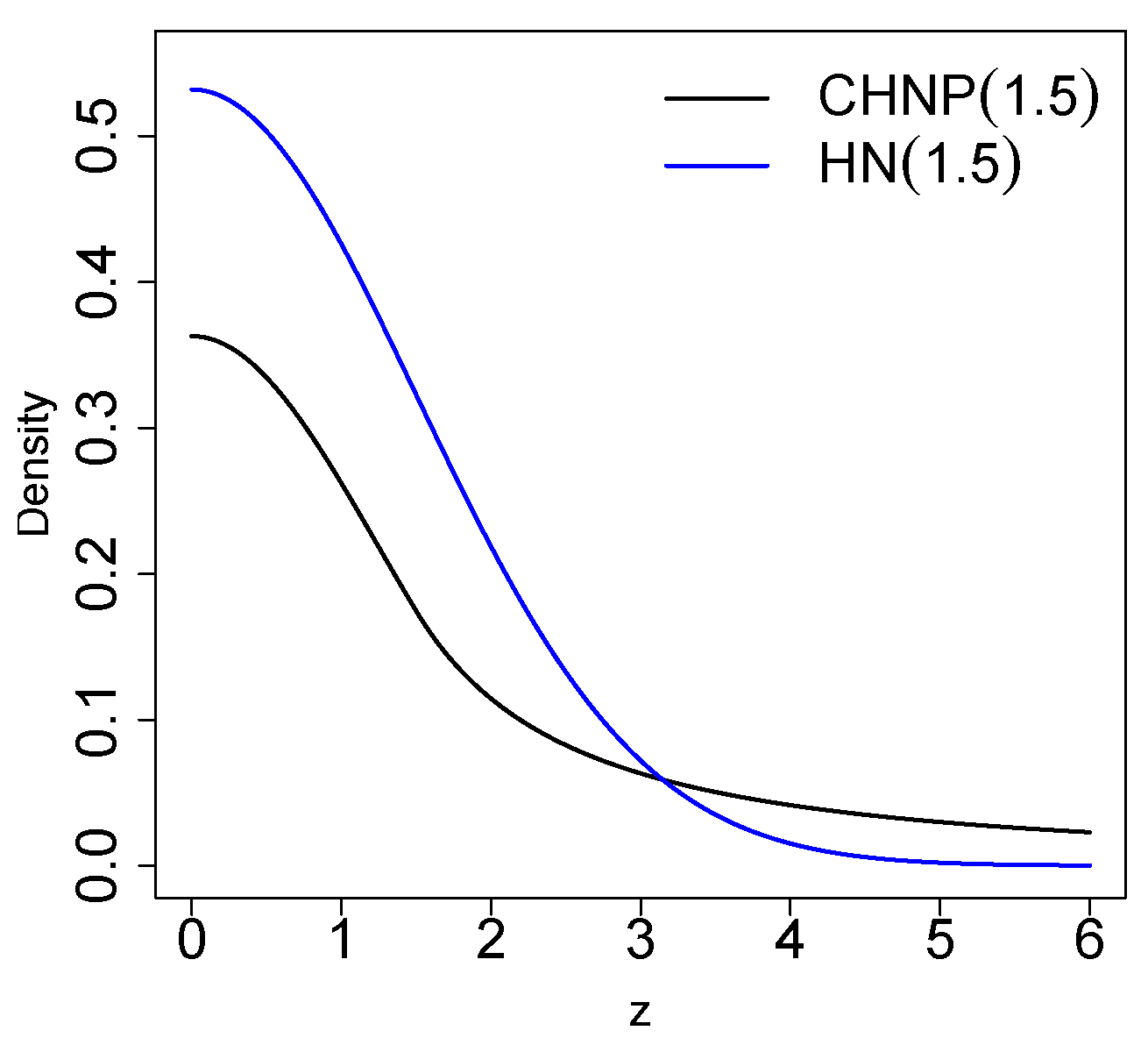
From Figure 1, it can be seen that the CHNP distribution has a heavier right tail than the HN distribution, although both have only one parameter. This is an important point with this methodology, in which we increase the weight of the right tail without increasing the parametric space. We also observe that the CHNP distribution maintains some of the properties of the HN model, such as its capacity to include zero. This is a very important characteristic, since the presence of zeros affects distribution modeling. Many parametric models found in the literature cannot be used for datasets containing zeros.

Figure 1. Comparison of HN and CHNP distributions.

2.2. Properties

This subsection presents some properties of the CHNP distribution, such as its mode, cdf, survival and risk functions, quantile function, median, and its coefficients of asymmetry and kurtosis.

Proposition 2.

The CHNP distribution is unimodal and is reached at zero.

Proof. 

Deriving with respect to z, we have

$$f_Z^{\prime }(z;\theta )=\left\{\begin{array}{cc}-\frac{(1+k)\sqrt{1+k}}{\Phi \left(\sqrt{1+k}\right){\theta }^3}z\varphi \left(\frac{\sqrt{1+k}}{\theta }z\right),\hfill & \mathrm{if}0\le z\le \theta ,\hfill \\ \\ -\frac{k(1+k){\theta }^k}{2\Phi \left(\sqrt{1+k}\right)}{z}^{-(2+k)},\hfill & \mathrm{if}\theta \le z<\infty .\hfill \end{array}\right.$$

We observe that for $0\le z\le \theta$, we have $-\frac{(1+k)\sqrt{1+k}}{\Phi \left(\sqrt{1+k}\right){\theta }^3}z\varphi \left(\frac{\sqrt{1+k}}{\theta }z\right)=0,$ so long as $z=0$, then the mode is 0.    □

Proposition 3.

Let $Z\sim CHNP\left(\theta \right)$ with $\theta >0$. Then, the cdf of Z is

$$F_Z(z;\theta )=\left\{\begin{array}{cc}\frac{1}{\Phi \left(\sqrt{1+k}\right)}\left(\Phi \left(\frac{\sqrt{1+k}}{\theta }z\right)-\frac{1}{2}\right),\hfill & if0\le z\le \theta ,\hfill \\ \\ 1-\frac{{\theta }^k{z}^{-k}}{2\Phi \left(\sqrt{1+k}\right)},\hfill & if\theta \le z<\infty .\hfill \end{array}\right.$$

(3)

Proof. 

Applying the definition of cdf directly, the result is obtained.    □

Corollary 1.

1. 

The survival function $s\left(t\right)$, which is the probability that an article will not fail before time t, is defined by $s\left(t\right)=1-F\left(t\right)$. The survival function for a $Z\sim CHNP\left(\theta \right)$ random variable is given by

$$s\left(t\right)=\left\{\begin{array}{cc}1-\frac{1}{\Phi \left(\sqrt{1+k}\right)}\left(\Phi \left(\frac{\sqrt{1+k}}{\theta }t\right)-\frac{1}{2}\right),\hfill & if0\le t\le \theta ,\hfill \\ \\ \frac{{\theta }^k{t}^{-k}}{2\Phi \left(\sqrt{1+k}\right)},\hfill & if\theta \le t<\infty .\hfill \end{array}\right.$$

2. 

The hazards function $h\left(t\right)$, defined by $h\left(t\right)=\frac{f\left(t\right)}{s\left(t\right)}$, for a $Z\sim CHNP\left(\theta \right)$ random variable, is given by

$$h\left(t\right)=\left\{\begin{array}{cc}\frac{\sqrt{1+k}\varphi \left(\frac{\sqrt{1+k}}{\theta }t\right)}{\theta \left(\Phi \left(\sqrt{1+k}\right)-\Phi \left(\frac{\sqrt{1+k}}{\theta }t\right)+\frac{1}{2}\right)},\hfill & if0\le t\le \theta ,\hfill \\ \\ \frac{k}{t},\hfill & if\theta \le t<\infty .\hfill \end{array}\right.$$

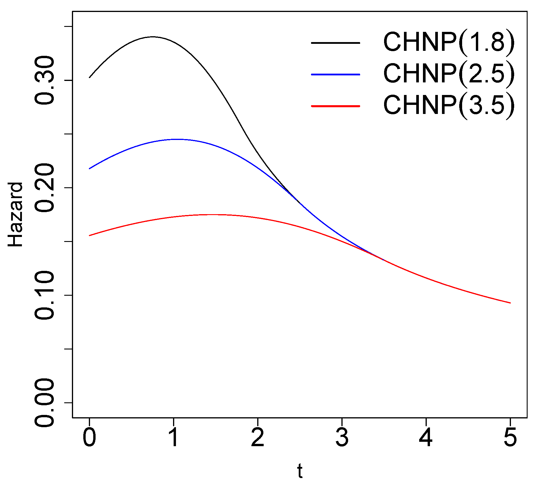
Figure 2 shows plots of the hazard function of the CHNP distribution, and Table 1 indicates that the hazard function is unimodal. We can analyze some monotonicity intervals of the hazard function of the CHNP distribution by resolving the following equation numerically.

$$\varphi \left(\frac{\sqrt{1+k}}{\theta }t\right)-\frac{\sqrt{1+k}t}{\theta }\left(\Phi \left(\sqrt{1+k}\right)-\Phi \left(\frac{\sqrt{1+k}t}{\theta }\right)+\frac{1}{2}\right)=0.$$

Figure 2. Plot of the hazard function $h\left(t\right)$ of the CHNP distribution with different values of parameter $\theta$.

Table 1. Monotonicity of the hazard function.

$\mathit{\theta }$	Increasing	Decreasing
1	$(0,0.4183847]$	$(0.4183847,\infty )$
$1.8$	$(0,0.7530924]$	$(0.7530924,\infty )$
$2.5$	$(0,1.045962]$	$(1.045962,\infty )$
$3.5$	$(0,1.464346]$	$(1.464346,\infty )$
5	$(0,1.673539]$	$(1.673539,\infty )$

Table 1 provides some numerical computations for calculating monotonicity intervals of the hazard function of the CHNP distribution for different parametric values.

Remark 2.

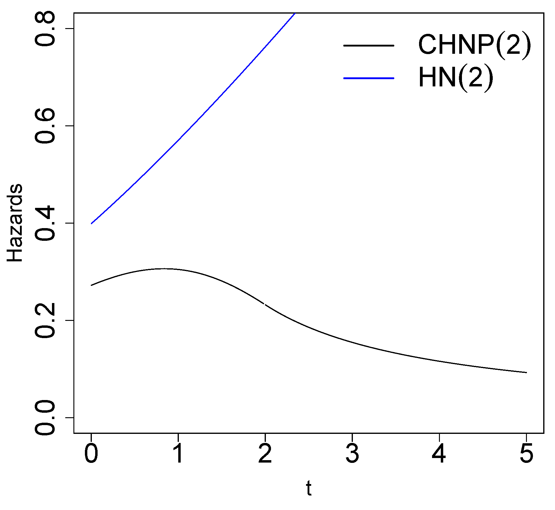
From Figure 3, it can be observed that the hazard function of the HN distribution is increasing, whereas the hazard function of the CHNP distribution is more flexible.

Figure 3. Comparison of hazard functions of the HN and CHNP distributions.

Right Tail of the CHNP Distribution

We know that any probability distribution, specified by its cdf $F\left(t\right)$ on the real numbers, has a heavy right tail (see Rolski et al. [21]) if

$$\begin{array}{c}\hfill \underset{t\to \infty }{lim\; sup}\left(-\frac{logs\left(t\right)}{t}\right)=0.\end{array}$$

The following result shows that the CHNP distribution has a heavy right tail.

Proposition 4.

The cdf of the random variable $T\sim CHNP\left(\theta \right)$ is a heavy-tailed distribution.

Proof. 

We have

$$\begin{array}{ccc}\hfill \underset{t\to \infty }{lim\; sup}\left(-\frac{logs\left(t\right)}{t}\right)& =& \underset{t\to \infty }{lim\; sup}\left(\frac{f_T(t;\sigma ,q)}{1-F_T(t;\sigma ,q)}\right)\hfill \\ & =& \underset{t\to \infty }{lim\; sup}\left(\frac{k}{t}\right)\hfill \\ & =& 0,\hfill \end{array}$$

where we have applied L’Hospital’s Rule once to obtain the result.    □

Remark 3.

In the case of a random variable $X\sim HN\left(\sigma \right)$, we have

$$\begin{array}{ccc}\hfill \underset{x\to \infty }{lim\; sup}\left(-\frac{logs\left(x\right)}{x}\right)& =& \underset{x\to \infty }{lim\; sup}\left(\frac{f_X(x;\sigma )}{1-F_X(x;\sigma )}\right)\hfill \\ & =& \underset{x\to \infty }{lim\; sup}\frac{\varphi \left(\frac{x}{\sigma }\right)}{\sigma \left(1-\Phi \left(\frac{x}{\sigma }\right)\right)}\hfill \\ & =& \underset{x\to \infty }{lim\; sup}\left(\frac{x}{{\sigma }^2}\right)\hfill \\ & =& \infty .\hfill \end{array}$$

Applying L’Hospital’s Rule twice, the result obtained indicates that the HN distribution does not have a heavy right tail; this is a reason for developing the CHNP distribution, which does have a heavy right tail.

Proposition 5.

Let $Z\sim CHNP\left(\theta \right)$. Then, the quantile function (Q) of the CHNP distribution is given by

$$Q\left(p\right)=\left\{\begin{array}{cc}\frac{\theta }{\sqrt{1+k}}{\Phi }^{-1}\left(p\Phi \left(\sqrt{1+k}\right)+\frac{1}{2}\right),\hfill & if0<p\le 0.4614636,\hfill \\ \\ \theta {\left(2\Phi \left(\sqrt{1+k}\right)(1-p)\right)}^{-1/k},\hfill & if0.4614636\le p<1.\hfill \end{array}\right.$$

(4)

Proof. 

Clearing z in the equation $p=F_Z(z;\theta )$, the result is obtained.    □

Corollary 2.

Let $Z\sim CHNP\left(\theta \right)$. Then, the median ($Me$) of the CHNP distribution is given by

$$Me=\frac{\theta }{{\Phi }^{1/k}\left(\sqrt{1+k}\right)}$$

(5)

We study the effects of the parameter $\theta$ on the coefficients of asymmetry and kurtosis defined by Galton [22] and Moors [23], respectively. These are based on the quantile function and are given in the following result.

Corollary 3.

Let $Z\sim CHNP\left(\theta \right)$; then, the coefficients of asymmetry ($\sqrt{{\beta }_1}$) and kurtosis (${\beta }_2$) are, respectively:

$$\sqrt{{\beta }_1}=\frac{Q\left(\frac{3}{4}\right)+Q\left(\frac{1}{4}\right)-2Q\left(\frac{2}{4}\right)}{Q\left(\frac{3}{4}\right)-Q\left(\frac{1}{4}\right)}=1.54737,$$

$${\beta }_2=\frac{Q\left(\frac{3}{8}\right)-Q\left(\frac{1}{8}\right)+Q\left(\frac{7}{8}\right)-Q\left(\frac{5}{8}\right)}{Q\left(\frac{3}{4}\right)-Q\left(\frac{1}{4}\right)}=5.648296,$$

where $Q(·)$ is the quantile function given in Equation (7). The value of the coefficient of kurtosis of the HN distribution is $1.176419$, while the value of the coefficient of kurtosis of the CHNP distribution is $5.648296$. In other words, the right tail of the CHNP distribution is heavier than the right tail of the HN distribution.

An algorithm exists to generate random numbers of the CHNP distribution (Algorithm 1).

Algorithm 1 The algorithm for simulating from the $Z\sim CHNP\left(\theta \right)$ can proceed as follows

1: Generate $Y\sim Uniform(0,1).$ 2: Compute $$Z=\left\{\begin{array}{cc}\frac{\theta }{\sqrt{1+k}}{\Phi }^{-1}\left(Y\Phi \left(\sqrt{1+k}\right)+\frac{1}{2}\right),\hfill & \mathrm{if}0<Y\le 0.4614636,\hfill \\ \theta {\left(2\Phi \left(\sqrt{1+k}\right)(1-Y)\right)}^{-1/k},& \mathrm{if}0.4614636\le Y<1,\end{array}\right.$$ (6)

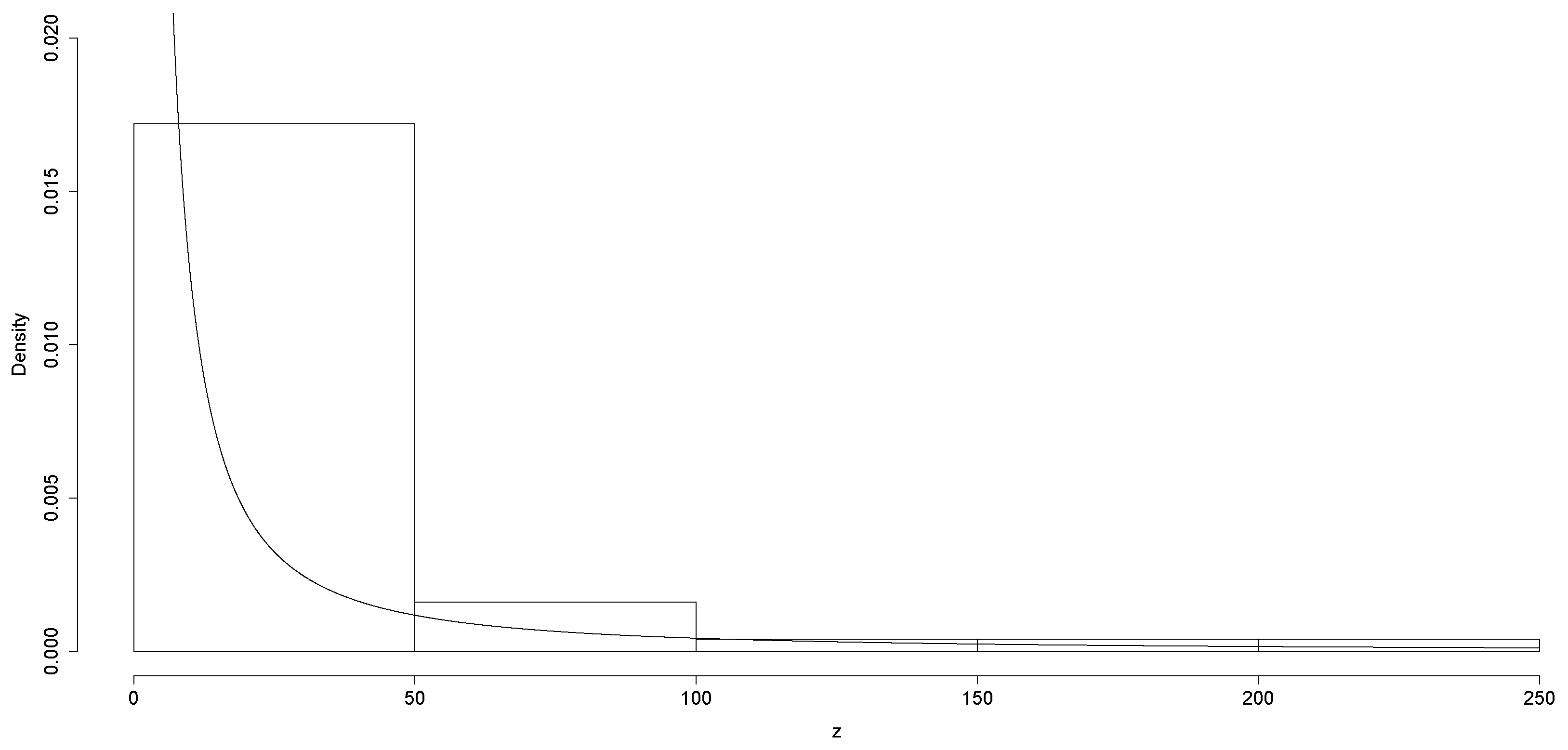
Using the R software package [24], R version 4.3.3, https://www.r-project.org/ (accessed on 15 January 2024), we generated a random sample of size $n=50$ from $Z\sim CHNP\left(\theta \right)$, shown in Figure 4. The codes in R are:

Figure 4. Histogram using a sample of size $n=50$ from density CHNP(2).

1:

Generate $y=runif(n,0,1)$

2:

$k=0.464288$

3:

Compute

$$\begin{array}{ccc}\hfill z& =& ifelse(y<0.4614636,\hfill \\ & & (2/sqrt(1+k\left)\right)\ast qnorm\left(\right(y\ast pnorm\left(sqrt\right(1+k\left)\right)+0.5\left)\right),\hfill \\ & & 2\ast (2\ast pnorm\left(sqrt(1+k)\right)\ast (1-y))(-1/k\left)\right)\hfill \end{array}$$

2.3. Actuarial Measure

Distributions with heavy tails are used to describe the risk exposure; for example, the quantile function is used in the area of actuarial statistics to define the value at risk (VaR). We discuss the VaR measure for the CHNP distribution. The VaR measure is also known as the quantile risk measure or the quantile premium principle and is specified with a given degree of confidence, which may be 90%, 95%, or 99%. The VaR of the random variable $Z\sim CHNP\left(\theta \right)$ is defined as (see Artzner [25] and Artzner et al. [26]):

$$Va{R}_p=Q\left(p\right)=\left\{\begin{array}{cc}\frac{\theta }{\sqrt{1+k}}{\Phi }^{-1}\left(p\Phi \left(\sqrt{1+k}\right)+\frac{1}{2}\right),\hfill & \mathrm{if}0<p\le 0.4614636,\hfill \\ \\ \theta {\left(2\Phi \left(\sqrt{1+k}\right)(1-p)\right)}^{-1/k},\hfill & \mathrm{if}0.4614636\le p<1,\hfill \end{array}\right.$$

(7)

Table 2 provides some numerical computations for the VaR_p measure of the CHNP($\theta$) distribution for different parametric values. Figure 5 shows graphs of the VaR_p measurement of the CHNP distribution for different values of parameter $\theta$.

Table 2. VaR_p measure and p is the significance level.

Model	p	VaRp	Model	p	VaRp
CHNP(0.5)	$0.90$	$20.73632$	CHNP(5)	$0.90$	$207.3632$
CHNP(0.5)	$0.95$	$92.27857$	CHNP(5)	$0.95$	$922.7857$
CHNP(0.5)	$0.99$	$2955.067$	CHNP(5)	$0.99$	$29,550.67$
CHNP(1)	$0.90$	$41.47265$	CHNP(8)	$0.90$	$331.7812$
CHNP(1)	$0.95$	$184.5571$	CHNP(8)	$0.95$	$1476.457$
CHNP(1)	$0.99$	$5910.134$	CHNP(8)	$0.99$	47,281.07
CHNP(3)	$0.90$	$124.4179$	CHNP(10)	$0.90$	$414.7265$
CHNP(3)	$0.95$	$553.6714$	CHNP(10)	$0.95$	$1845.571$
CHNP(3)	$0.99$	$17,730.4$	CHNP(10)	$0.99$	59,101.34

Figure 5. Plots of the VaR measure of the CHNP distribution with different values of parameter $\theta$.

3. Parameter Estimation

In this section we present two methods for estimating the parameter $\theta$, the first based on percentiles and the second on ML.

3.1. A Method Based on Percentiles

Let $z_1\le z_2\le ,\dots ,\le z_n$ be an ordered random sample derived from the $CHNP\left(\theta \right)$ distribution. We assume that $z_m\le \theta \le z_{m+1}$. Using the percentiles, the parameter $\theta$ can be estimated as the p-th percentile, where $p=F\left(\theta \right)$ and $k=0.464288$.

From Equation (3), we have

$$p=P(Z\le \theta )=F_Z\left(\theta \right)=\frac{1}{\Phi \left(\sqrt{1+k}\right)}\left(\Phi \left(\frac{\sqrt{1+k}}{\theta }\theta \right)-\frac{1}{2}\right)=0.436223$$

We have an estimate of the p-th percentile (see Klugman et al. [27]) given by

$$\tilde{\theta }=(1-h)z_m+h{z}_{m+1},$$

where $m=\left[\right(n+1\left)p\right]$, $h=(n+1)p-m$ and $\left[a\right]$ indicates the largest integer less than or equal to a.

3.2. ML Estimation

Let $z_1\le z_2\le ,\dots ,\le z_n$ be an ordered random sample derived from the $CHNP\left(\theta \right)$ distribution and $z_m\le \theta \le z_{m+1}$; the likelihood function can be written as

$$L(\theta ;z_1,\dots ,z_n)=\prod _{i=1}^m\frac{\sqrt{1+k}}{\Phi \left(\sqrt{1+k}\right)\theta }\varphi \left(\frac{\sqrt{1+k}}{\theta }{z}_i\right)\prod _{i=m+1}^n\frac{k{\theta }^k}{2\Phi \left(\sqrt{1+k}\right)}{z}_i^{-(1+k)}.$$

The log-likelihood function can be written as

$$\ell \left(\theta \right)=c_1-mlog\left(\theta \right)-\frac{m(1+k)}{2{\theta }^2}\overline{z_m^2}+k(n-m)log\left(\theta \right)-(1+k)\sum _{i=m+1}^{n}log\left(z_i\right),$$

where $c_1=\frac{m}{2}log(1+k)-mlog\left(\Phi \left(\sqrt{1+k}\right)\right)-\frac{m}{2}log\left(2\pi \right)+(n-m)log\left(k\right)-(n-m)log(2\Phi \left(\sqrt{1+k}\right))$ and ${\displaystyle {\overline{z^2}}_m=\frac{1}{m}\sum _{i=1}^m{z}_i^2}$.

Differentiating $\ell \left(\theta \right)$ with respect to $\theta$, we have

$$\frac{\partial \ell \left(\theta \right)}{\partial \theta }=-\frac{m}{\theta }+\frac{m(1+k)}{{\theta }^3}\overline{z_m^2}+\frac{k(n-m)}{\theta }.$$

Hence, the solution of the equation $\frac{\partial \ell \left(\theta \right)}{\partial \theta }=0$ is

$${\widehat{\theta }}_m=\sqrt{\frac{(1+k)m\overline{z_m^2}}{(1+k)m-kn}},kn<(1+k)m.$$

(8)

For each m, $m=1,2,...,n-1$, we evaluate ${\widehat{\theta }}_m$; if it is found that $z_m\le {\widehat{\theta }}_m\le z_{m+1}$, then the ML estimate of $\theta$ is $\widehat{\theta }={\widehat{\theta }}_m$.

Lemma 1.

Let $Z\sim CHNP\left(\theta \right)$. Then,

(i) 

${\int }_0^{\theta }\left({\displaystyle \frac{{\partial }^2}{\partial {\theta }^2}}log{f}_1^{*}(z;\theta )\right)f_1^{*}(z;\theta )dz=\frac{1}{2\Phi \left(\sqrt{1+k}\right){\theta }^2}\left(2+3k-4\Phi \left(\sqrt{1+k}\right)\right)$,

(ii) 

${\int }_{\theta }^{\infty }\left({\displaystyle \frac{{\partial }^2}{\partial {\theta }^2}}log{f}_2^{*}(z;\theta )\right)f_2^{*}(z;\theta )dz=-\frac{k}{2\Phi \left(\sqrt{1+k}\right){\theta }^2}$,

where $f_1^{*}(z;\theta )=\frac{\sqrt{1+k}}{\Phi \left(\sqrt{1+k}\right)\theta }\varphi \left(\frac{\sqrt{1+k}}{\theta }z\right)$ and $f_2^{*}(z;\theta )=\frac{k{\theta }^k}{2\Phi \left(\sqrt{1+k}\right)}{z}^{-(1+k)}.$

Proof. 

Results $\left(i\right)$ and $\left(ii\right)$ are obtained by performing their respective calculations.    □

Proposition 6.

Let $z_1\le z_2\le ,\dots ,\le z_n$ be an ordered random sample derived from the $CHNP\left(\theta \right)$ distribution; we assume that $z_m\le \theta \le z_{m+1}$. Then, the Fisher information $\left(I_F\right)$ for the θ parameter of the CHNP distribution is given by

$$I_F\left(\theta \right)=\frac{1}{2\Phi \left(\sqrt{1+k}\right){\theta }^2}\left[2m(2\Phi \left(\sqrt{1+k}\right)-3k-1)+2nk-(n-2m)k^2\right].$$

(9)

Proof. 

After calculations and applying the Leibniz Theorem (see Casella and Berger [28], Section 2.4), we have

$$\begin{array}{ccc}\hfill I_F\left(\theta \right)& =& \mathbb{E}\left[{\left({\displaystyle \frac{\partial \ell \left(\theta \right)}{\partial \theta }}\right)}^2\right]\hfill \\ & =& \sum _{i=1}^m{\int }_0^{\theta }{\left({\displaystyle \frac{\partial }{\partial \theta }}log{f}_1^{*}(z_i;\theta )\right)}^2{f}_1^{*}(z_i;\theta )d{z}_i+\sum _{i=m+1}^n{\int }_{\theta }^{\infty }{\left({\displaystyle \frac{\partial }{\partial \theta }}log{f}_2^{*}(z_i;\theta )\right)}^2{f}_2^{*}(z_i;\theta )d{z}_i\hfill \\ & =& -\sum _{i=1}^m{\int }_0^{\theta }\left({\displaystyle \frac{{\partial }^2}{\partial {\theta }^2}}log{f}_1^{*}(z_i;\theta )\right)f_1^{*}(z_i;\theta )d{z}_i-\sum _{i=m+1}^n{\int }_{\theta }^{\infty }\left({\displaystyle \frac{{\partial }^2}{\partial {\theta }^2}}log{f}_2^{*}(z_i;\theta )\right)f_2^{*}(z_i;\theta )d{z}_i+\frac{k(1-k)(n-2m)}{2\Phi \left(\sqrt{1+k}\right){\theta }^2}\hfill \\ & =& -m{\int }_0^{\theta }\left({\displaystyle \frac{{\partial }^2}{\partial {\theta }^2}}log{f}_1^{*}(z;\theta )\right)f_1^{*}(z;\theta )dz-(n-m){\int }_{\theta }^{\infty }\left({\displaystyle \frac{{\partial }^2}{\partial {\theta }^2}}log{f}_2^{*}(z;\theta )\right)f_2^{*}(z;\theta )dz+\frac{k(1-k)(n-2m)}{2\Phi \left(\sqrt{1+k}\right){\theta }^2}.\hfill \end{array}$$

Then, applying Lemma 1, the result is obtained.    □

Hence, for large samples, the ML estimator, $\widehat{\theta }$, is asymptotically normal; that is,

$$\widehat{\theta }\stackrel{\mathcal{L}}{⟶}N(\theta ,I_F^{-1}\left(\theta \right)),$$

resulting that the asymptotic variance of the ML estimator $\widehat{\theta }$ is the inverse of Fisher’s information is given in Equation (9), i.e.,

$$Var\left(\widehat{\theta }\right)\approx \frac{2\Phi \left(\sqrt{1+k}\right){\theta }^2}{2m(2\Phi \left(\sqrt{1+k}\right)-3k-1)+2nk-(n-2m)k^2}.$$

3.3. Simulation Study

To examine the behavior of the ML estimation, a simulation study is presented to assess the performance of the ML estimator for parameter $\theta$ of the CHNP distribution.

Algorithm 1 given in Section 2.2 can be used to generate random numbers from the CHNP distribution. The simulation analysis was carried out by generating 1000 samples from the CHNP distribution, of sizes $n=50$, 100, 150, and 200.

Table 3 shows the empirical bias (Bias), the mean of the standard errors (SEs), the root of the empirical mean squared error (RMSE), and the 95% coverage probability (CP) based on the asymptotic distribution for the ML estimator of parameter $\theta$. As Table 3 shows, the performance of the estimations improves as n increases.

Table 3. Bias, SE, RMSE, and CP for the CHNP model with sample sizes 50, 100, 150, and 200.

$\mathit{\theta }$	n	Bias	SE	RMSE	CP
1	50	0.0420	0.2492	0.2632	0.9398
	100	0.0157	0.1720	0.1758	0.9456
	150	0.0130	0.1402	0.1433	0.9458
	200	0.0130	0.1402	0.1227	0.9458
2	50	0.0695	0.4952	0.5255	0.9391
	100	0.0337	0.3443	0.3564	0.9442
	150	0.0216	0.2791	0.2863	0.9420
	200	0.0142	0.2408	0.2449	0.9454
3	50	0.1067	0.7441	0.7928	0.9381
	100	0.0631	0.5176	0.5361	0.9447
	150	0.0373	0.4193	0.4340	0.9411
	200	0.0242	0.3617	0.3700	0.9415
4	50	0.0242	0.3617	1.0656	0.9415
	100	0.0802	0.6897	0.7206	0.9413
	150	0.0593	0.5599	0.5703	0.9468
	200	0.0361	0.4829	0.4930	0.9465

4. Applications

In this section, we show three applications, the first with simulated data and the others with real datasets. To compare the models, we use the Akaike information criterion AIC (see Akaike [29]) and the Bayesian information criterion BIC (see Schwarz [30]).

4.1. Numerical Application

In this numerical application, we use the same 50 simulated data used for the graph in Figure 4; these data were generated from the CHNP(2) distribution. The data are shown in Table 4.

Table 4. 50 simulated data.

0.01445457	0.01925126	0.04748003	0.12887746	0.19892610	0.53610582
0.70568085	0.72404104	0.78969039	0.82392295	0.84496216	0.90191984
0.92244296	1.21130369	1.26907096	1.28636763	1.30668599	1.35093138
1.42432950	1.65535034	1.72375311	1.84486889	1.96947573	2.10059341
2.14786935	2.68653223	2.71026918	2.73182813	3.10511668	3.41038988
3.57082832	4.44431142	5.09754874	5.21285944	5.60614295	6.62777414
8.60098244	9.32670082	10.85377372	14.28964739	20.51202824	25.16157611
27.74187053	60.16026763	65.41449211	71.33535927	87.67022926	102.51836463
183.21141945	215.76829133

The descriptive statistics for these data are given in Table 5, where CS is the coefficient of asymmetry of the sample and CK is the coefficient of kurtosis. A high coefficient of kurtosis of $6.477$ is observed; we generated these data with $\theta =2$, meaning that the right tail of the data is very heavy.

Table 5. Descriptive statistics for 50 simulated data from the CHNP(2) model.

n	Median	Mean	Variance	CS	CK
50	2.417	19.474	1936.553	0.651	6.477

The first object of this numerical example is to use the estimation methods given in Section 3.

• A method based on percentiles. For this example, $p=0.436223$. We have $m=\left[\right(n+1\left)p\right]=\left[22.24737\right]=22$ and $h=22.24737-22=0.24737$. Thus, the estimator of $\theta$ is $\tilde{\theta }=(1-0.24737)z_{22}+0.24737\ast z_{23}=1.875693$, where $z_{22}=1.84486889$ and $z_{23}=1.96947573$.
• ML estimation. Using the value of $m=22$ found with the previous method, we calculate the estimator given in Equation (8). This gives us ${\widehat{\theta }}_{22}=1.994828$. We observe that the ratio $z_{22}\le {\widehat{\theta }}_{22}\le z_{23}$ is not satisfied. Therefore, we must use another value for m, for example $m=23$; with this, we obtain ${\widehat{\theta }}_{23}=1.9913$, and now we observe that the ratio $z_{23}\le {\widehat{\theta }}_{23}\le z_{24}$ is satisfied, where $z_{23}=1.96947573$ and $z_{24}=2.10059341$. Thus, the ML estimate of $\theta$ is $\widehat{\theta }={\widehat{\theta }}_{23}=1.9913$.

The second objective of this numerical example is to compare the fit with the Pareto model, since this model has a heavy right tail. Table 6 shows the ML estimations for the parameters of the CHNP model and the Pareto model. Table 6 also shows the values of the AIC and BIC criteria for each model.

Table 6. Fifty simulated data: Model, ML estimates, AIC, and BIC values.

Model	ML Estimates	AIC	BIC
CHNP($\theta$)	$\widehat{\theta }=1.991$	325.641	329.855
Pareto($\theta ,\alpha$)	$\widehat{\theta }=0.015\widehat{\alpha }=0.188$	378.785	380.697

The lowest values of the AIC and BIC criteria correspond to the CHNP model, meaning that the CHNP model offers a better fit for these data than the Pareto model. This was to be expected since the data were simulated from the CHNP model. The above values for the measures indicate that the CHNP model has its own shape and may be difficult to replace by any other known model with a heavy right tail.

4.2. Application to Income Data

This dataset comes from the U.S. Survey of Consumer Finances (SCF), a nationally representative sample that contains extensive information on assets, liabilities, income, and demographic characteristics of those sampled (potential U.S. customers). It contains a random sample of 500 households with positive incomes, which were interviewed in the 2004 survey. The variable of interest is the annual income of the family in thousands of USD divided by the number of household members. The descriptive statistics for these data are given in Table 7.

Table 7. Descriptive statistics for income data.

n	Median	Mean	Variance	CS	CK
500	21.125	216.709	11,270,001	0.435	1.655

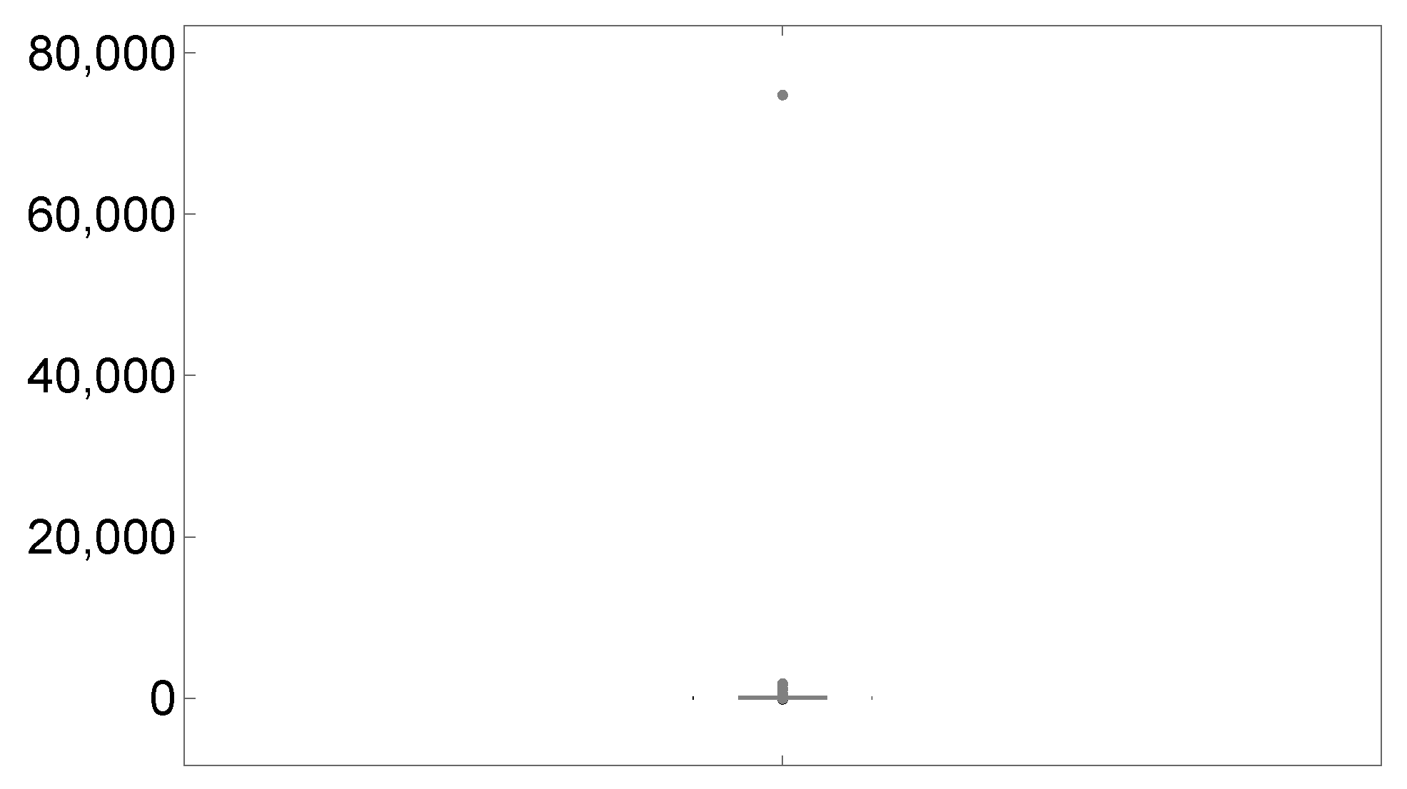
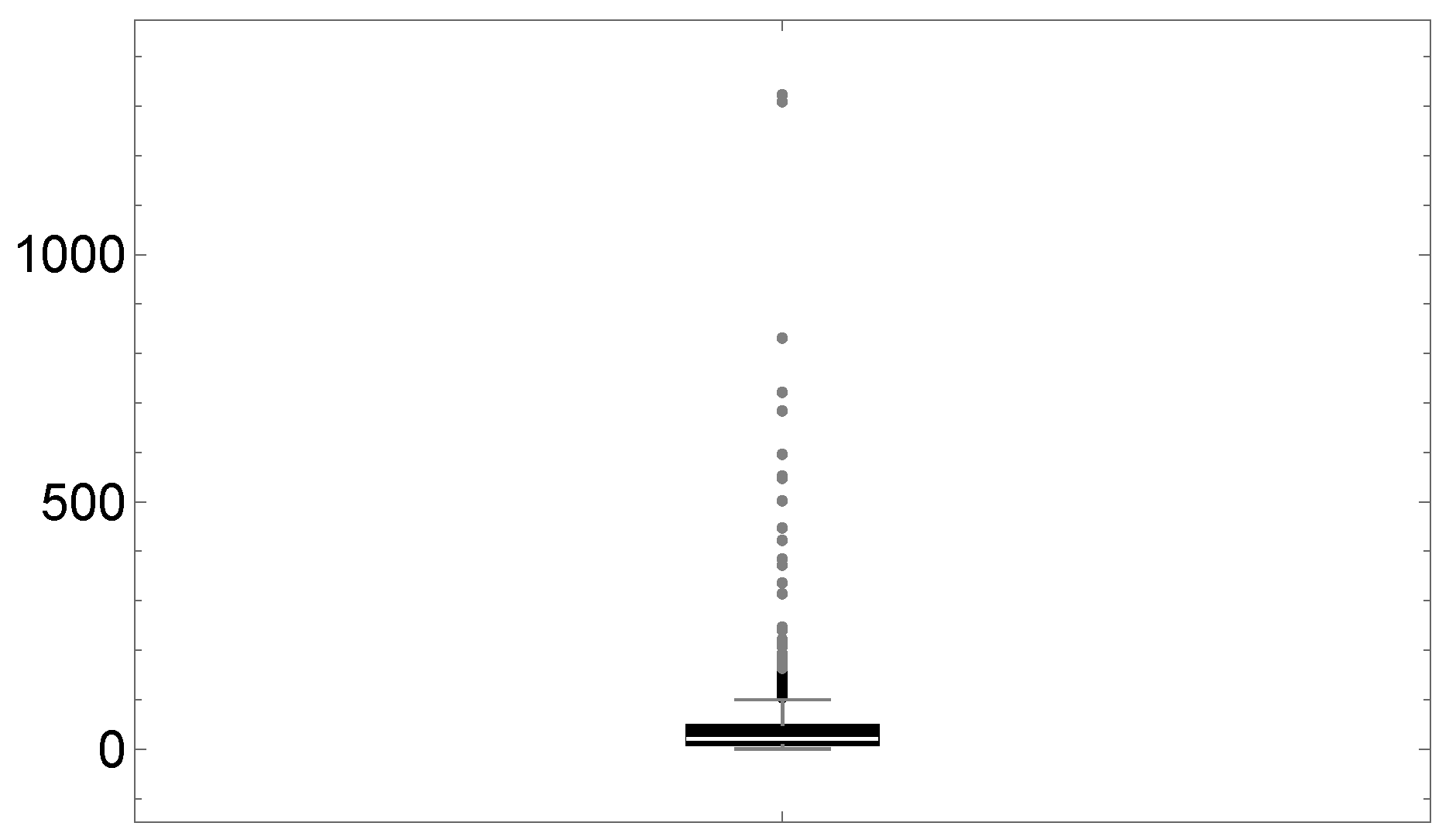
Figure 6 presents a boxplot that shows one very extreme datum, while Figure 7 shows a boxplot of the dataset after removing the extreme datum in order to show the other outliers, which cannot be seen in the boxplot of Figure 6. These atypical data make the right tail heavier. It may be noted that the majority of the observations are around USD 21,125 per capita per family, but there is one very atypical value representing an income of USD 75 million. Because the Pareto distribution has a heavy right tail, we use it to compare its fit to the income data with the fit of the CHNP distribution.

Figure 6. Boxplot for income data.

Figure 7. Boxplot for income data without extreme data.

Table 8 shows the ML estimates for the parameters of the Pareto, CEP, and CHNP models, as well as the values of the AIC and BIC criteria for each model.

Table 8. ML estimates for the income data with corresponding standard errors (in parentheses), AIC and BIC values.

Model	ML Estimates	AIC	BIC
CHNP($\theta$)	$\widehat{\theta }=19.370\left(1.978\right)$	4937.446	4947.875
CEP($\theta$)	$\widehat{\theta }=21.446\left(1.675\right)$	5049.790	5054.005
Pareto($\theta ,\alpha$)	$\widehat{\theta }=0.065\left(0.001\right)$
	$\widehat{\alpha }=0.171\left(0.008\right)$	5867.910	5876.339

It can be observed that the lowest values of the AIC and BIC criteria correspond to the CHNP model, meaning that the CHNP model offers a better fit for these data than the CEP and Pareto models.

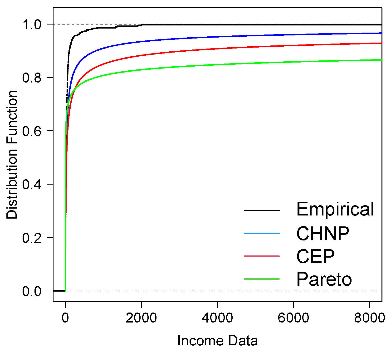
Figure 8 shows the empirical cdf with estimated cdfs of the CHNP, CEP, and Pareto models. Note the good fit of the CHNP model with the income data.

Figure 8. Plots of the empirical cdf, with estimated CHNP cdf, estimated CEP cdf, and estimated Pareto cdf models.

Table 9 presents VaR estimates for the CHNP, CEP, and Pareto distributions at the following levels: 0.5, 0.6, 0.7, 0.8, 0.9, and 0.95. We know that the model with higher VaR values has a heavier tail. Table 9 shows that the Pareto model has a heavier tail than the CHNP and CEP models at the highest levels. Table 8 and Figure 9 also show the good fit of the CHNP model with the income data. According to the selection criteria of the AIC and BIC models, the CHNP model fits the income data better than the CEP and Pareto models.

Table 9. Comparison of the VaR of different models for income data.

Model∖Significance	$0.5$	$0.6$	$0.7$	$0.8$	$0.9$	$0.95$
CHNP($\widehat{\theta }$)	25.086	40.565	75.379	180.519	803.325	3574.872
CEP($\widehat{\theta }$)	31.813	60.186	136.919	436.094	3159.847	22,895.580
Pareto($\widehat{\theta },\widehat{\alpha }$)	3.744	13.805	74.248	795.165	45,800.120	2,638,007

Figure 9. Plots of the empirical VaR, plots of the VaR for CHNP, CEP, and Pareto models.

4.3. Application to Expenditure Data

The data were obtained from the Medical Expenditure Panel Survey (MEPS), carried out by the US Agency for Healthcare Research and Quality in the civil population. The variable of interest consists of expenditure amounts for ambulatory visits (EXPENDOP). The data can be found in Frees [31]. The descriptive statistics for these data are given in Table 10.

Table 10. Descriptive statistics for expenditure data.

n	Median	Mean	Variance	CS	CK
75	2.5608	4.9559	87.030	0.079	1.165

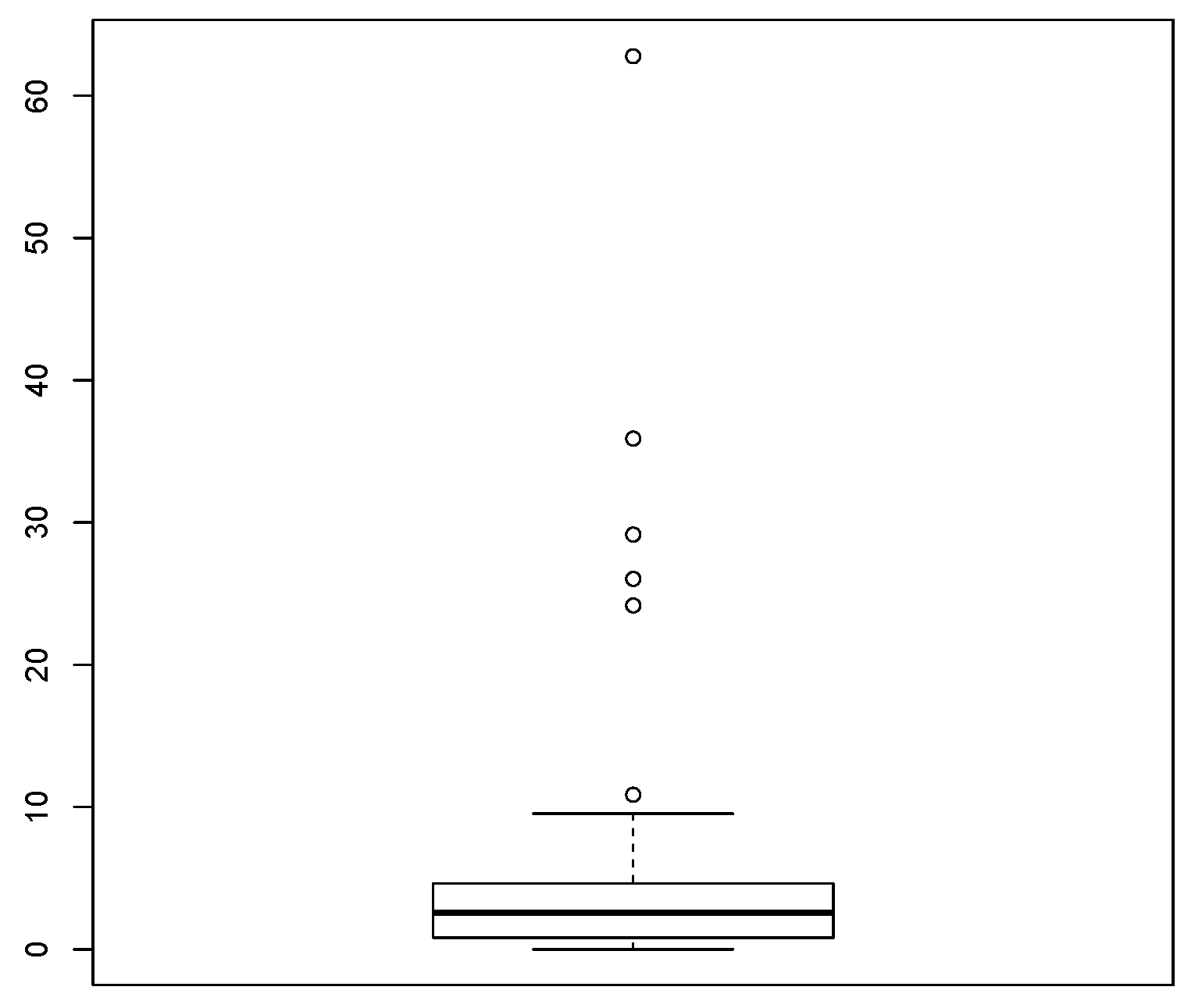
Figure 10 presents a boxplot that shows extreme data, one of which is very extreme. These outliers make the right tail heavy. The dataset has three observations with zero cost; it therefore cannot be fitted with the Pareto model, and we only compared CHNP with the CEP model. These two models can be fitted to datasets containing zero observations.

Figure 10. Boxplot for expenditure data.

Table 11 shows the ML estimates for the parameters of the CEP and CHNP models, as well as the values of the AIC and BIC criteria for each model.

Table 11. ML estimates for the expenditure data with corresponding standard errors, AIC and BIC values.

Model	ML Estimates	AIC	BIC
CHNP($\theta$)	$\widehat{\theta }=2.042\left(0.533\right)$	392.609	399.244
CEP($\theta$)	$\widehat{\theta }=2.007\left(0.469\right)$	405.183	411.818

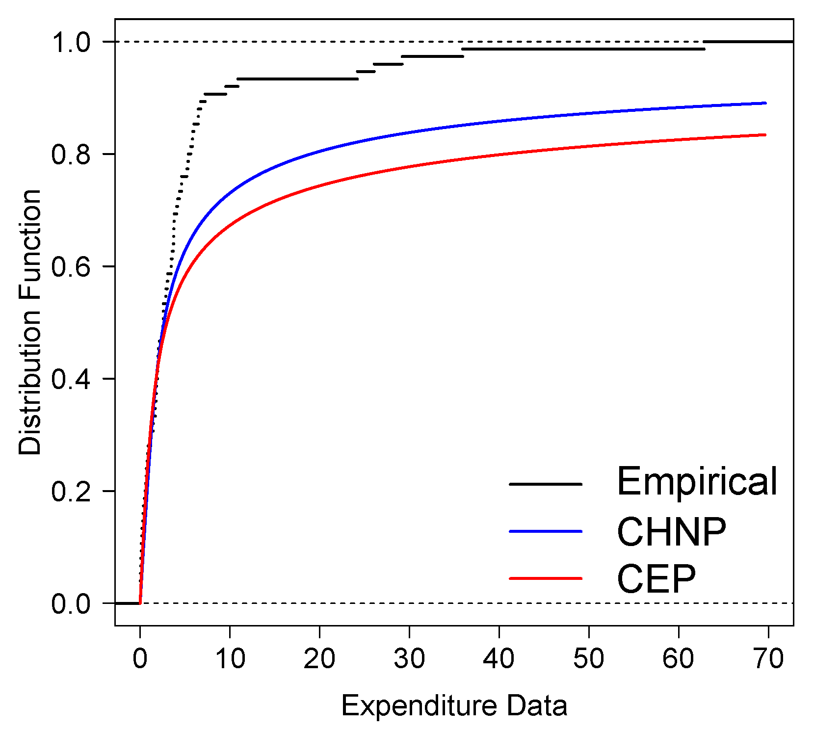
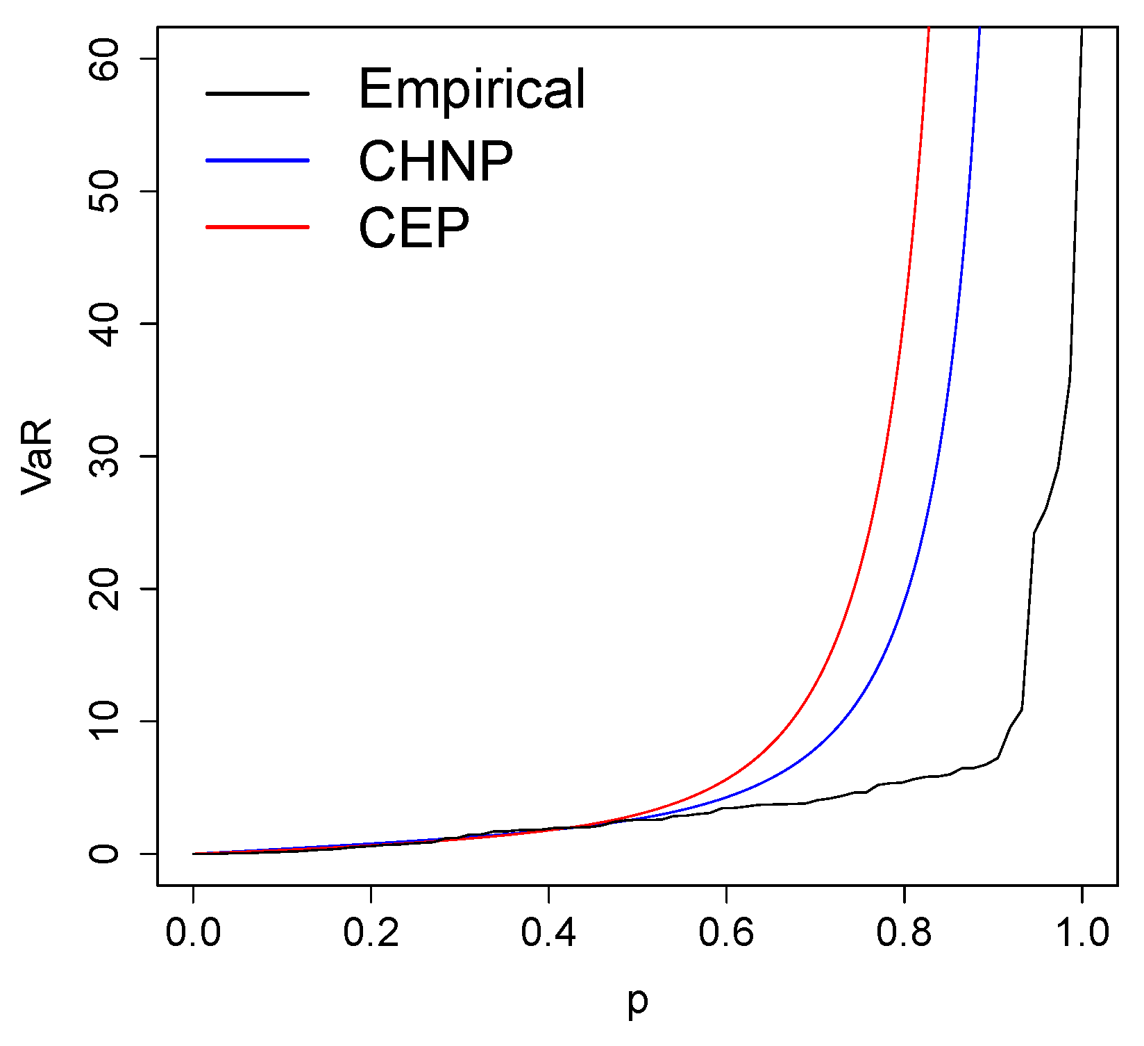
It can be observed that the lowest values of the AIC and BIC criteria correspond to the CHNP model, meaning that the CHNP model offers a better fit for these data than the CEP model. Figure 11 and Figure 12 show the empirical cdf and VaR with estimated cdfs of the CHNP and CEP models. Note the good fit of the CHNP model with the expenditure data.

Figure 11. Plots of the empirical cdf, with estimated CHNP cdf and estimated CEP cdf models.

Figure 12. Plots of the empirical VaR and plots of the VaR for CHNP and CEP models.

5. Concluding Remarks

This paper presents a study of the CHNP model, which was generated by the same methodology introduced by Cooray and Ananda [11]. The CHNP model has only one parameter, making it an attractive competitor with various one-parameter models used in actuarial statistics. The CHNP model is a viable alternative for fitting data with extreme observations. Some other characteristics of the CHNP model are:

• The CHNP model has a heavy right tail, as is shown by Proposition 4.
• The support of the CHNP model contains zero. It is a property that is very important for modeling datasets containing zero.
• Cdf, risk function, and quantile function are explicit and are represented by known functions.
• The VaR risk measure is explicit in the CHNP model; in the applications with real data, it is compared with the VaR risk measure of the CEP and Pareto models.
• The applications with income and expenditure data show that the CHNP model provides a better fit than the CEP and Pareto models; it is also observed that the VaR of the CHNP model is closer to the empirical VaR than the VaR of the CEP and Pareto models.
• One reviewer noted the importance of performing a comparison of estimation methods, including Bayesian inference. As we have Fisher’s information for the parameter $\theta$, we can use it in Jeffrey’s prior to perform Bayesian inference. However, a detailed investigation of the performance of Bayesian estimation is beyond the scope of the present paper.

References

- Beirlant, J.; Teugels, J.L.; Vynckier, P. Practical Analysis of Extreme Values; Leuven University Press: Leuven, Belgium, 1996. [Google Scholar]
- Beirlant, J.; Joossens, E.; Segers, J. Generalized Pareto fit to the society of actuaries’ large claims database. N. Am. Actuar. J. 2004, 8, 108–111. [Google Scholar] [CrossRef]
- Resnick, S.I. Discussion of the Danish data on large fire insurance losses. ASTIN Bull. 1997, 27, 139–151. [Google Scholar] [CrossRef]
- Pareto, V. Cours d’Éconimie Politique; F. Rouge: Laussanne, Swizerland, 1897. [Google Scholar]
- Arnold, B.C. Pareto Distributions, 2nd ed.; Chapman & Hall: New York, NY, USA, 2015. [Google Scholar]
- Azzalini, A. A class of distributions which includes the normal ones. Scand. J. Stat. 1985, 12, 171–178. [Google Scholar]
- Henze, N. A probabilistic representation of the Skew-Normal distribution. Scand. J. Stat. 1986, 4, 271–275. [Google Scholar]
- Cooray, K.; Ananda, M.M.A. A Generalization of the Half-Normal Distribution with Applications to Lifetime Data. Commun. Stat.—Theory Methods 2008, 37, 1323–1337. [Google Scholar] [CrossRef]
- Olmos, N.M.; Varela, H.; Gómez, H.W.; Bolfarine, H. An extension of the half-normal distribution. Stat. Pap. 2012, 53, 875–886. [Google Scholar] [CrossRef]
- Olmos, N.M.; Varela, H.; Bolfarine, H.; Gómez, H.W. An extension of the generalized half-normal distribution. Stat. Pap. 2014, 55, 967–981. [Google Scholar] [CrossRef]
- Cooray, K.; Ananda, M.M.A. Modeling actuarial data with a composite lognormal-Pareto model. Scand. Actuar. J. 2005, 5, 321–334. [Google Scholar] [CrossRef]
- Scollnik, D.P.M. On composite lognormal–Pareto models. Scand. Actuar. J. 2007, 7, 20–33. [Google Scholar] [CrossRef]
- Cooray, K.; Cheng, C.I. Bayesian estimators of the lognormal–Pareto composite distribution. Scand. Actuar. J. 2015, 6, 500–515. [Google Scholar] [CrossRef]
- Ciumara, R. An actuarial model based on the composite Weibull–Pareto distribution. Math. Rep. 2006, 8, 401–414. [Google Scholar]
- Cooray, K. The Weibull–Pareto composite family with applications to the analysis of unimodal failure rate data. Commun. Stat.—Theory Methods 2009, 38, 1901–1915. [Google Scholar] [CrossRef]
- Teodorescu, S. On the truncated composite lognormal–Pareto model. Math. Rep. 2010, 12, 71–84. [Google Scholar]
- Teodorescu, S.; Panaitescu, E. On the truncated composite Weibull–Pareto model. Math. Rep. 2009, 11, 259–273. [Google Scholar]
- Teodorescu, S.; Vernic, R. Some composite exponential–Pareto models for actuarial prediction. Rom. J. Econ. Forecast. 2009, 12, 82–100. [Google Scholar]
- Scollnik, D.P.M.; Sun, C. Modeling with Weibull–Pareto models. N. Am. Actuar. J. 2012, 16, 260–272. [Google Scholar] [CrossRef]
- Calderín-Ojeda, E.; Azpitarte, F.; Gómez-Déniz, E. Modelling income data using two extensions of the exponential distribution. Physica A 2016, 461, 756–766. [Google Scholar] [CrossRef]
- Rolski, T.; Schmidli, H.; Schmidt, V.; Teugel, J. Stochastic Processes for Insurance and Finance; John Wiley & Sons: Hoboken, NJ, USA, 1999. [Google Scholar]
- Galton, F. Enquiries into Human Faculty and Its Development; Macmillan & Company: London, UK, 1883. [Google Scholar]
- Moors, J.J.A. A quantile alternative for kurtosis. J. R. Stat. Soc. Ser. D Stat. 1988, 37, 25–32. [Google Scholar] [CrossRef]
- R Core Team. R: A Language and Environment for Statistical Computing; R Foundation for Statistical Computing: Vienna, Austria, 2022; Available online: https://www.R-project.org/ (accessed on 12 January 2024).
- Artzner, P. Application of coherent risk measures to capital requirements in insurance. N. Am. Actuar. J. 1999, 3, 11–25. [Google Scholar] [CrossRef]
- Artzner, P.; Delbaen, F.; Eber, J.-M.; Heath, D. Coherent measures of risk. Math. Financ. 1999, 9, 203–228. [Google Scholar] [CrossRef]
- Klugman, S.A.; Panjer, H.H.; Willmot, G.E. Loss Models: From Data to Decisions, 4th ed.; Wiley: New York, NY, USA, 1998. [Google Scholar]
- Casella, G.; Berger, R. Statistical Inference, 2nd ed.; Cengage Learning: Boston, MA, USA, 2002. [Google Scholar]
- Akaike, H. A new look at the statistical model identification. IEEE Trans. Autom. Control 1074, 19, 716–723. [Google Scholar] [CrossRef]
- Schwarz, G. Estimating the dimension of a model. Ann. Stat. 1978, 6, 461–464. [Google Scholar] [CrossRef]
- Frees, E.W. Regression Modeling with Actuarial and Financial Applications; Cambridge University Press: Cambridge, UK, 2010. [Google Scholar]
Disclaimer/Publisher’s Note: The statements, opinions and data contained in all publications are solely those of the individual author(s) and contributor(s) and not of MDPI and/or the editor(s). MDPI and/or the editor(s) disclaim responsibility for any injury to people or property resulting from any ideas, methods, instructions or products referred to in the content. |
© 2024 by the authors. Licensee MDPI, Basel, Switzerland. This article is an open access article distributed under the terms and conditions of the Creative Commons Attribution (CC BY) license (https://creativecommons.org/licenses/by/4.0/).