
Process Capability Evaluation Using Capability Indices as a Part of Statistical Process Control


Abstract
1. Introduction
1.1. Manufacturing Process Capability Analysis
- It verifies the suitability of the designed process to ensure the required quality attributes of the product;
- It enables the likelihood of nonconformity to be estimated and optimises production planning;
- It is an essential indicator for planning the maintenance of production equipment;
- It is the basis for planning corrective actions and assessing their effectiveness;
- It provides evidence to the customer that the product has been produced under stable manufacturing conditions that ensure regular compliance with the prescribed quality criteria.
1.1.1. Manufacturing Process Capability Analysis Using the Histogram
1.1.2. Manufacturing Process Capability Analysis Using the Probability Plot
1.1.3. Manufacturing Process Capability Analysis Using the Control Chart
1.1.4. Manufacturing Process Capability Analysis Using Design of Experiments
1.1.5. Manufacturing Process Capability Analysis Using Capability Indices
- Selection of the quality characteristic
- The process capability is evaluated based on a specific quality characteristic of the manufactured or intermediate product. It is necessary to select the characteristic whose value reflects the success of the process under consideration and is decisive for the product. The customer may specify this characteristic or be critical regarding a desired product characteristic or a link to the following production process.
- 2.
- Measurement system analysis
- Before data collection, it is necessary to analyse the measurement system of the selected quality characteristics and verify its acceptability, as an unacceptable measurement system may lead to incorrect results of the process capability assessment [24]. Many authors, such as McNeese and Klein [25], Persijn and Nuland [26], Mittag [27], Pearn and Liao [28] and Hsu et al. [29], have pointed out that the capability of the chosen characteristic’s measurement system affects the process’s calculated capability.
- 3.
- Data collection
- When monitoring the capability of an existing process, data collection should be carried out over a sufficiently long period to reflect all the usual sources of variability that affect the process (e.g., operator turnover, feedstock supply, maintenance). During this period, several products shall be chosen from the production process at regular intervals, and the quality characteristics shall be measured. It is recommended that the number of subgroups should be at least 25, with a range of 4–5 values in each subgroup [23]. The range of selection is essential because it affects the accuracy of the index calculation.
- 4.
- Verification of the prerequisites of the quality characteristic
- Verification of the Normality
- An indicative assessment of whether the measured values conform to a normal distribution can be obtained from the shape of the histogram constructed (Section 1.1.1) or the probability plot (Section 1.1.2). An accurate way of verifying normality is to use statistical tests, for example, Anderson–Darling’s test [30] or the Kolmogorov–Smirnov nonparametric goodness of fit [31], which are based on the empirical distribution function, the Shapiro–Wilk test [32], the Ryan–Joiner test [33] correlation-based test or the Jarque–Bera test [34] based on the measures of skewness and kurtosis. Different tests of normality are based on different principles and have different strengths. Therefore, some tests may reject normality, and others may not. Multiple normality tests and one of the graphical tools, e.g., a probability plot, should be used simultaneously for a comprehensive assessment of normality. If the examined data are not normally distributed, it is possible to transform them to a normal distribution or use modified indices calculations considering the relevant distribution.
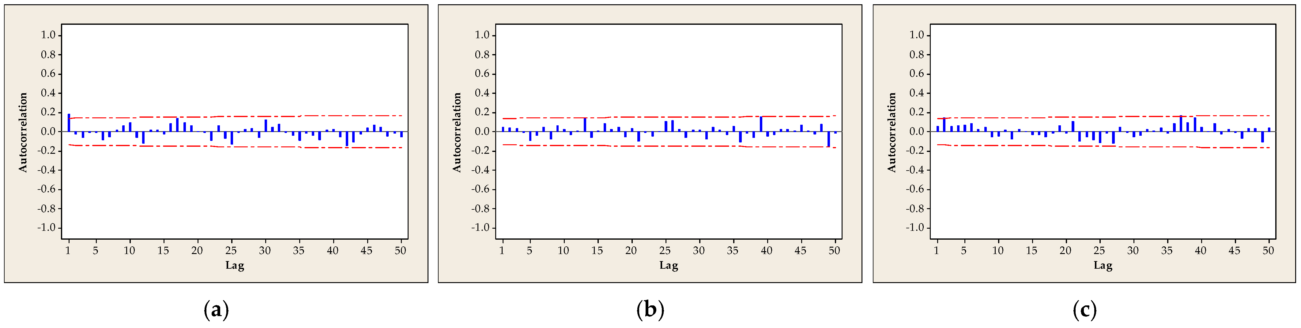
- Data Independence Verification
- The classical approach to process capability analysis assumes that the measured data are independent. An autocorrelation function was used to verify the independence of the data in the examined datasets [19]. Some processes, such as biological or chemical processes, in particular, violate the assumption of independence. A procedure for assessing process capability for auto-correlated data can be found in studies, e.g., Zhang [35], Vännman and Kulahci [36], Mohamadi et al. [37] or Sun et al. [38].
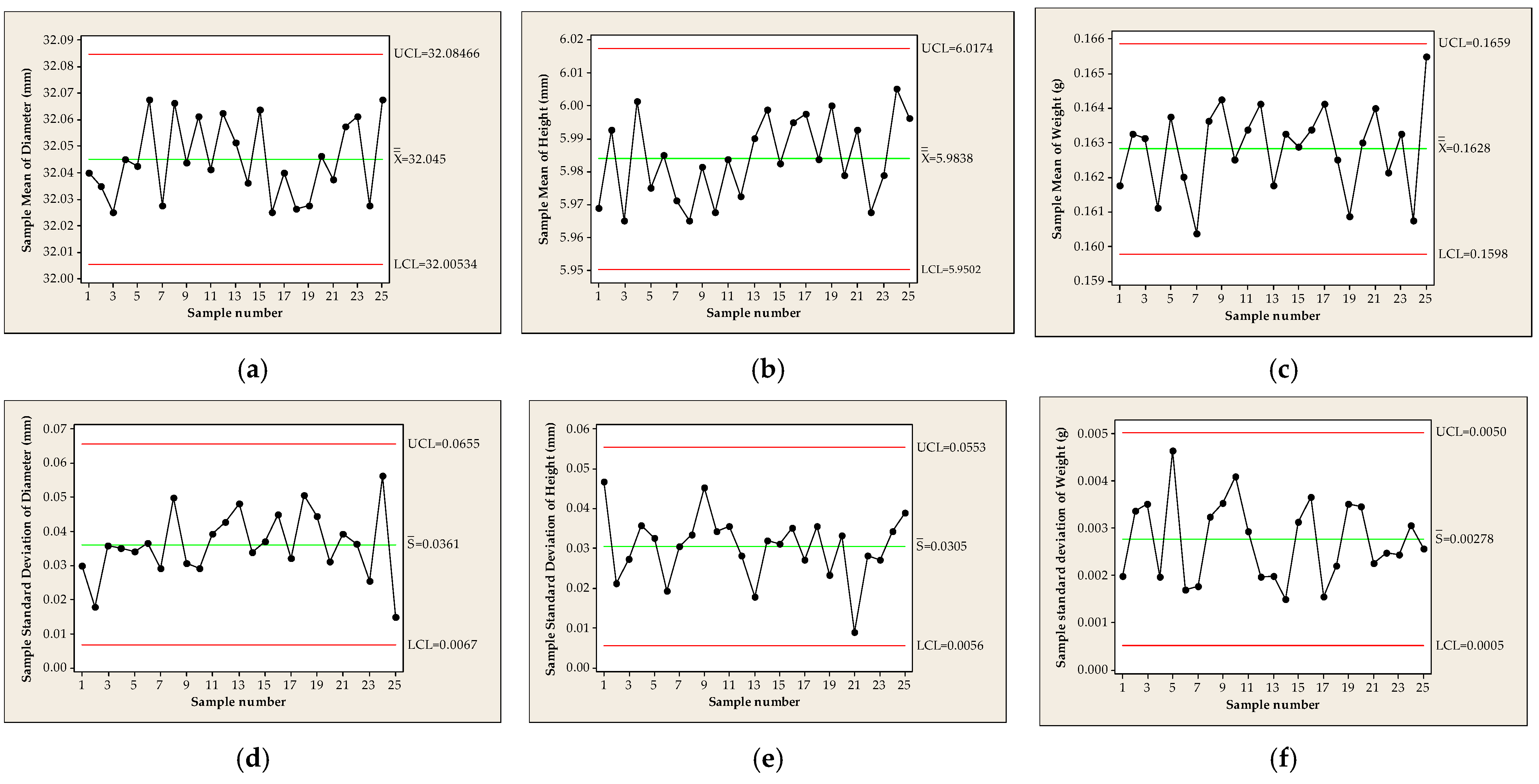
- Verification of the Process Stability
- Data must be collected from a process in the state of statistical control, in which the variability of the observed quality characteristic is due only to the influence of random causes. Suppose the control charts analysis shows that the process is not in the state of statistical control. In that case, it is necessary to analyse the observed process, detect the definable causes [15] that caused the instability, eliminate it and create conditions such that its influence is not repeated. Pyzdek and Keller [39] point out that applying process capability methods to processes outside of statistical control leads to unreliable estimates of process capability and should never be done. Process capability represents the performance of a process only in a state of statistical control [40].
- 5.
- Calculation of capability indices and comparison with required values
- The final step in assessing process capability is to calculate and compare the appropriate capability indices to the required values. The most commonly used indices for quality characteristics from a normal distribution are Cp and Cpk. The first assesses a process’s potential, and the second assesses the actual capability to deliver products that consistently meet tolerance limits. In addition, the Cpm and Cpmk indices assess the ability of the process to achieve the target mean of the quality characteristic being monitored. Section 2.3, Section 2.4 and Section 2.5 deal with these capability indices in more detail. Supplementing the calculated capability indices with graphs, as recommended by Vänman [41,42], improves the assessment of process capability.
1.2. The Purpose of the Study
2. Materials and Methods
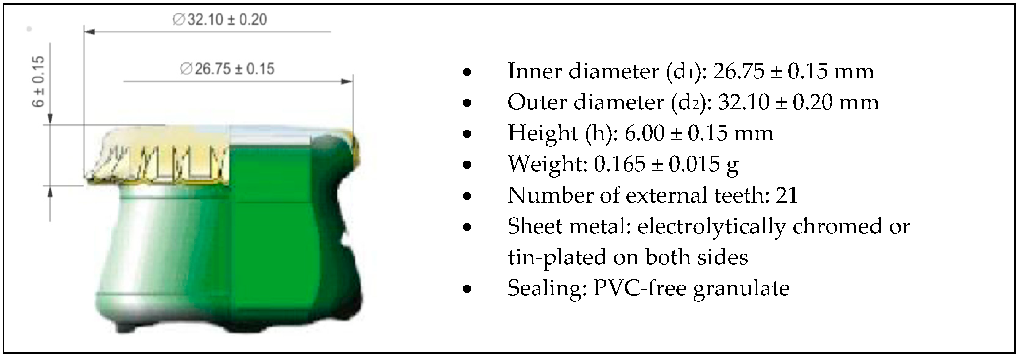
2.1. Description of the Crown Cap Manufacturing Process
2.2. Selection of the Quality Characteristic
2.3. Capability Indices and their Calculation
2.3.1. Process Variability
- Using the pooled standard deviation based on a standard one-way analysis of variance without (4) or with a bias correction (5);
- Using an average subgroup range Ri (6);
- Using an average subgroup standard deviation without a bias correction (7),
2.3.2. Capability Index Cp
2.3.3. Capability Index Ca
2.3.4. Capability Index Cpk
- If Cpk < 0, the process is centred outside the specification limits and produces nonconforming outputs;
- If Cpk = 0, the process is centred on one of the specification limits;
- If Cpk < 1.0, the process is unable to comply with the prescribed values;
- If Cpk ≥ 1.25, the process is a fit for normal products;
- If Cpk ≥ 1.45, the newly established manufacturing process or established manufacturing process for safety-related products is capable;
- If Cpk ≥ 1.67, the newly established manufacturing process for safety-related products is well capable, nonconforming output may occur, but the chances are excellent that it will be detected;
- If Cpk = 2.0, high confidence level of conforming process output, assuming control charts are used regularly.
2.3.5. Capability Index Cpm
2.3.6. Capability Index C*pm
2.3.7. Capability Index Cpmk
2.4. Confidence Intervals for Capability Indices
2.5. Summary of the Development of the Capability Indices
3. Results and Discussion
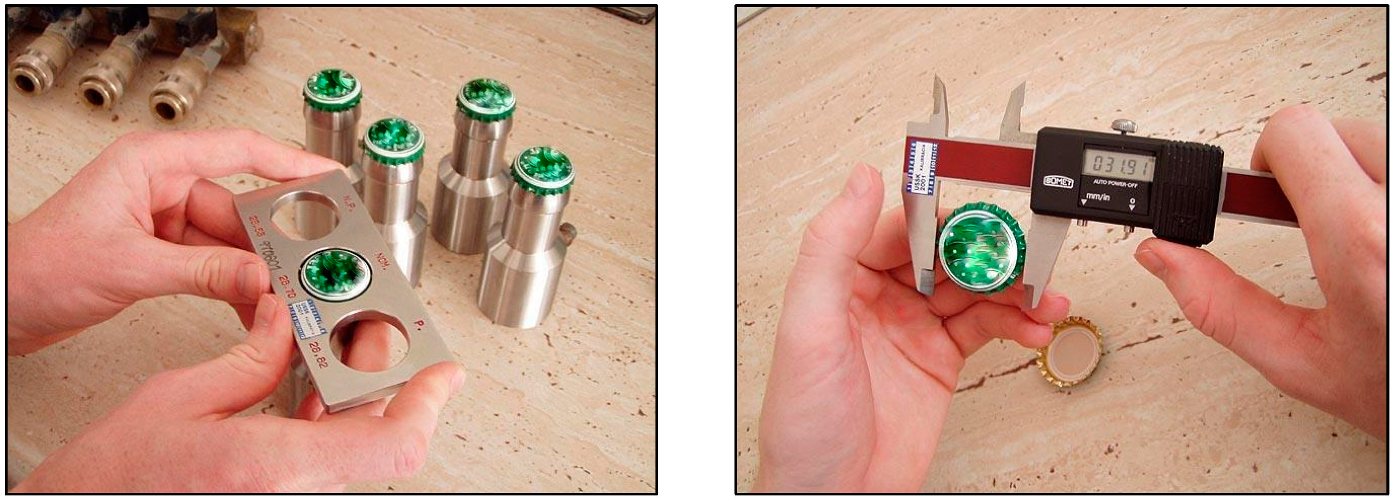
3.1. Measurement System Analysis
3.2. Assessment of the Capability of the Crown Cap Manufacturing Process
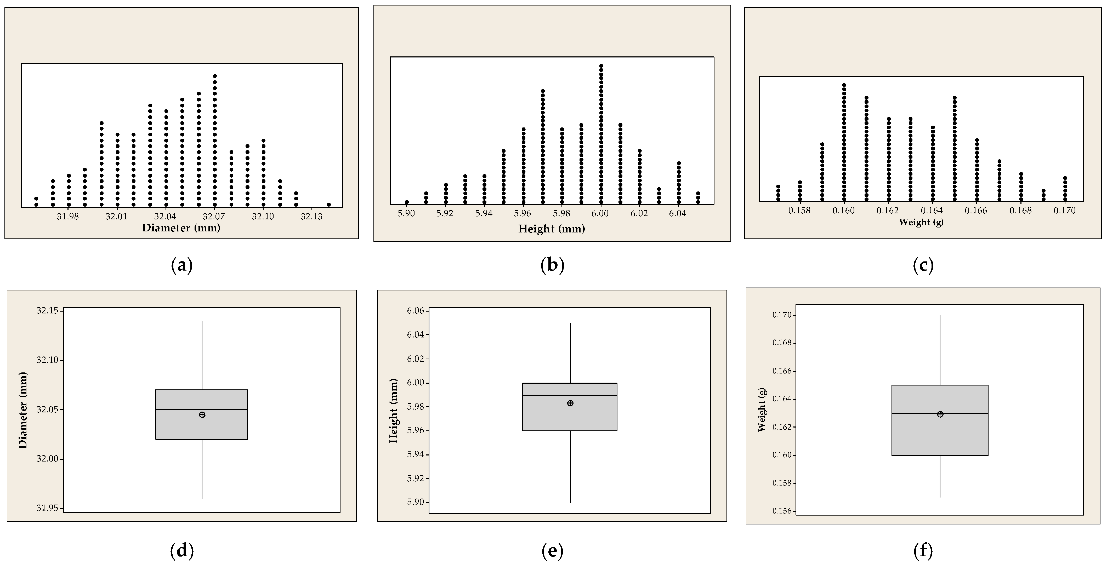
3.2.1. Data Collection and Review of Measured Datasets
3.2.2. Verification of Prerequisites for the Selection of Appropriate Capability Indices
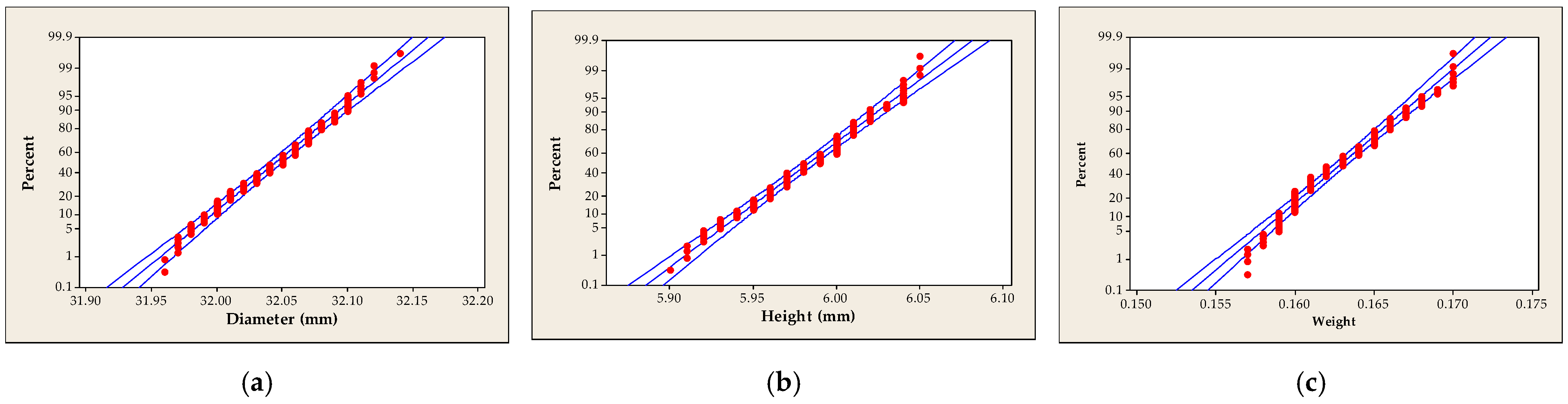
Verification of the Normality
Data Independence Verification
Verification of the Process Stability
3.2.3. Calculation of the Capability Indices and Comparison with the Required Value
Process Capability Assessment for the Quality Characteristic Diameter
Process Capability Assessment for the Quality Characteristic Height
Process Capability Assessment for the Quality Characteristic Weight
4. Conclusions
Author Contributions
Funding
Data Availability Statement
Conflicts of Interest
Appendix A

| Sample Number | Quality Characteristics | Crown Cap Number | |||||||
|---|---|---|---|---|---|---|---|---|---|
| 1 | 2 | 3 | 4 | 5 | 6 | 7 | 8 | ||
| 1 | Diameter | 32.07 | 32.02 | 32.07 | 32.03 | 32.02 | 32.05 | 31.99 | 32.07 |
| Height | 6.00 | 5.94 | 6.04 | 6.00 | 6.00 | 5.99 | 5.93 | 5.91 | |
| Weight | 0.164 | 0.162 | 0.162 | 0.158 | 0.160 | 0.162 | 0.164 | 0.162 | |
| 2 | Diameter | 32.06 | 32.03 | 32.01 | 32.02 | 32.06 | 32.04 | 32.03 | 32.03 |
| Height | 5.96 | 5.97 | 5.99 | 5.98 | 6.00 | 5.93 | 6.01 | 6.02 | |
| Weight | 0.167 | 0.161 | 0.170 | 0.161 | 0.162 | 0.162 | 0.161 | 0.162 | |
| 3 | Diameter | 32.05 | 32.06 | 32.01 | 32.00 | 32.02 | 32.08 | 31.97 | 32.01 |
| Height | 5.99 | 5.97 | 5.94 | 6.01 | 5.94 | 5.93 | 5.97 | 5.97 | |
| Weight | 0.170 | 0.159 | 0.164 | 0.166 | 0.161 | 0.163 | 0.161 | 0.161 | |
| 4 | Diameter | 32.04 | 32.03 | 32.01 | 32.00 | 32.04 | 32.05 | 32.09 | 32.10 |
| Height | 5.99 | 5.97 | 6.05 | 5.98 | 6.05 | 6.03 | 5.97 | 5.97 | |
| Weight | 0.165 | 0.160 | 0.159 | 0.161 | 0.160 | 0.163 | 0.160 | 0.161 | |
| 5 | Diameter | 32.06 | 32.05 | 32.00 | 32.06 | 32.02 | 32.00 | 32.05 | 32.10 |
| Height | 5.97 | 5.93 | 5.96 | 5.98 | 5.99 | 6.04 | 5.95 | 5.98 | |
| Weight | 0.167 | 0.160 | 0.169 | 0.160 | 0.169 | 0.160 | 0.167 | 0.158 | |
| 6 | Diameter | 32.04 | 32.01 | 32.05 | 32.10 | 32.11 | 32.11 | 32.07 | 32.05 |
| Height | 5.97 | 6.00 | 5.99 | 5.95 | 6.00 | 5.97 | 6.00 | 6.00 | |
| Weight | 0.161 | 0.162 | 0.160 | 0.16 | 0.164 | 0.162 | 0.165 | 0.161 | |
| 7 | Diameter | 32.07 | 32.06 | 32.02 | 32.01 | 32.03 | 31.98 | 32.04 | 32.01 |
| Height | 6.00 | 6.00 | 5.94 | 5.98 | 5.92 | 5.95 | 5.99 | 5.99 | |
| Weight | 0.160 | 0.159 | 0.162 | 0.169 | 0.164 | 0.160 | 0.159 | 0.160 | |
| 8 | Diameter | 32.10 | 32.04 | 32.00 | 32.00 | 32.07 | 32.08 | 32.10 | 32.14 |
| Height | 5.95 | 6.00 | 6.00 | 5.98 | 5.91 | 5.99 | 5.93 | 5.96 | |
| Weight | 0.158 | 0.165 | 0.166 | 0.168 | 0.163 | 0.166 | 0.162 | 0.161 | |
| 9 | Diameter | 32.09 | 32.07 | 32.05 | 32.03 | 32.03 | 31.99 | 32.03 | 32.06 |
| Height | 6.00 | 6.00 | 5.97 | 6.03 | 5.92 | 5.92 | 6.04 | 5.97 | |
| Weight | 0.163 | 0.169 | 0.165 | 0.163 | 0.170 | 0.162 | 0.162 | 0.160 | |
| 10 | Diameter | 32.08 | 32.07 | 32.06 | 32.07 | 32.10 | 32.06 | 32.05 | 32.00 |
| Height | 5.92 | 5.97 | 6.04 | 5.98 | 5.96 | 5.96 | 5.96 | 5.95 | |
| Weight | 0.161 | 0.168 | 0.161 | 0.160 | 0.170 | 0.159 | 0.160 | 0.161 | |
| 11 | Diameter | 32.04 | 32.03 | 32.02 | 32.06 | 32.07 | 32.07 | 31.96 | 32.07 |
| Height | 6.04 | 5.95 | 5.97 | 6.04 | 5.96 | 5.97 | 5.97 | 5.97 | |
| Weight | 0.164 | 0.163 | 0.168 | 0.169 | 0.166 | 0.163 | 0.160 | 0.164 | |
| 12 | Diameter | 32.05 | 32.00 | 32.00 | 32.08 | 32.10 | 32.11 | 32.09 | 32.07 |
| Height | 5.98 | 5.95 | 6.00 | 5.97 | 5.96 | 5.97 | 6.02 | 5.93 | |
| Weight | 0.164 | 0.168 | 0.164 | 0.165 | 0.161 | 0.163 | 0.164 | 0.164 | |
| 13 | Diameter | 32.00 | 32.03 | 32.10 | 32.01 | 32.01 | 32.10 | 32.12 | 32.04 |
| Height | 6.01 | 5.98 | 6.00 | 5.97 | 6.00 | 6.00 | 5.96 | 6.00 | |
| Weight | 0.159 | 0.162 | 0.160 | 0.161 | 0.164 | 0.162 | 0.165 | 0.161 | |
| 14 | Diameter | 32.04 | 31.99 | 32.01 | 32.06 | 32.09 | 32.05 | 32.00 | 32.05 |
| Height | 5.99 | 6.05 | 6.00 | 6.02 | 5.98 | 6.01 | 6.00 | 5.94 | |
| Weight | 0.166 | 0.163 | 0.162 | 0.161 | 0.164 | 0.163 | 0.164 | 0.163 | |
| 15 | Diameter | 32.04 | 32.04 | 32.03 | 32.12 | 32.05 | 32.03 | 32.11 | 32.09 |
| Height | 6.00 | 5.97 | 6.01 | 6.01 | 5.92 | 5.96 | 5.99 | 6.00 | |
| Weight | 0.168 | 0.159 | 0.166 | 0.163 | 0.160 | 0.164 | 0.160 | 0.163 | |
| 16 | Diameter | 32.04 | 32.05 | 31.97 | 32.04 | 32.04 | 32.10 | 31.98 | 31.98 |
| Height | 6.01 | 6.02 | 6.02 | 5.93 | 5.95 | 6.02 | 6.00 | 6.01 | |
| Weight | 0.162 | 0.165 | 0.166 | 0.157 | 0.165 | 0.166 | 0.167 | 0.159 | |
| 17 | Diameter | 32.06 | 32.06 | 32.04 | 32.02 | 32.01 | 32.05 | 32.09 | 31.99 |
| Height | 6.01 | 6.00 | 6.01 | 5.96 | 5.95 | 6.02 | 6.01 | 6.02 | |
| Weight | 0.166 | 0.165 | 0.164 | 0.161 | 0.165 | 0.163 | 0.165 | 0.164 | |
| 18 | Diameter | 32.01 | 31.97 | 32.09 | 32.07 | 31.98 | 32.09 | 32.02 | 31.98 |
| Height | 5.93 | 6.01 | 6.02 | 6.01 | 6.01 | 5.96 | 5.99 | 5.94 | |
| Weight | 0.164 | 0.160 | 0.165 | 0.165 | 0.162 | 0.163 | 0.159 | 0.162 | |
| 19 | Diameter | 32.00 | 31.97 | 32.03 | 32.09 | 32.07 | 32.07 | 31.99 | 32.00 |
| Height | 6.01 | 6.01 | 6.04 | 5.97 | 6.00 | 5.99 | 5.97 | 6.04 | |
| Weight | 0.157 | 0.160 | 0.161 | 0.167 | 0.158 | 0.161 | 0.158 | 0.165 | |
| 20 | Diameter | 32.06 | 32.05 | 32.02 | 32.06 | 31.99 | 32.08 | 32.03 | 32.08 |
| Height | 6.02 | 5.99 | 5.98 | 6.03 | 5.93 | 5.97 | 5.95 | 5.98 | |
| Weight | 0.160 | 0.165 | 0.165 | 0.157 | 0.165 | 0.160 | 0.166 | 0.166 | |
| 21 | Diameter | 31.99 | 32.03 | 32.01 | 32.00 | 32.10 | 32.03 | 32.08 | 32.06 |
| Height | 6.00 | 5.98 | 5.98 | 6.00 | 5.99 | 6.00 | 5.99 | 6.00 | |
| Weight | 0.166 | 0.163 | 0.161 | 0.164 | 0.162 | 0.163 | 0.165 | 0.168 | |
| 22 | Diameter | 32.08 | 32.02 | 32.00 | 32.07 | 32.07 | 32.03 | 32.09 | 32.10 |
| Height | 5.96 | 6.00 | 5.99 | 5.97 | 5.98 | 5.98 | 5.95 | 5.91 | |
| Weight | 0.165 | 0.166 | 0.162 | 0.159 | 0.163 | 0.160 | 0.160 | 0.162 | |
| 23 | Diameter | 32.07 | 32.07 | 32.06 | 32.06 | 32.05 | 32.05 | 32.02 | 32.11 |
| Height | 5.97 | 6.04 | 5.96 | 5.96 | 5.98 | 5.97 | 5.96 | 5.99 | |
| Weight | 0.165 | 0.163 | 0.161 | 0.161 | 0.167 | 0.160 | 0.164 | 0.165 | |
| 24 | Diameter | 31.98 | 32.04 | 32.02 | 32.08 | 32.05 | 31.96 | 31.97 | 32.12 |
| Height | 5.94 | 5.94 | 5.97 | 6.02 | 6.02 | 6.02 | 6.01 | 6.01 | |
| Weight | 0.159 | 0.157 | 0.159 | 0.160 | 0.167 | 0.163 | 0.161 | 0.160 | |
| 25 | Diameter | 32.07 | 32.06 | 32.06 | 32.09 | 32.07 | 32.08 | 32.07 | 32.04 |
| Height | 6.03 | 5.95 | 6.04 | 6.04 | 6.00 | 6.00 | 5.95 | 5.96 | |
| Weight | 0.161 | 0.164 | 0.165 | 0.166 | 0.167 | 0.170 | 0.166 | 0.165 | |
References
- ISO 9000:2015; Quality Management Systems—Fundamentals and Vocabulary. ISO: Geneva, Switzerland, 2015.
- Terek, M.; Hrnčiarová, Ľ. Štatistické Riadenie Kvality, 1st ed.; Iura Edition: Bratislava, Slovakia, 2004; ISBN 978-80-89047-97-0. [Google Scholar]
- Montgomery, D.C. Introduction to Statistical Quality Control, 6th ed.; Wiley: Hoboken, NJ, USA, 2009; ISBN 978-0-470-16992-6. [Google Scholar]
- Tošenovský, J.; Noskievičová, D. Statistické Metody pro Zlepšování Jakosti; Montanex: Ostrava, Czech Republic, 2000; ISBN 978-80-7225-040-0. [Google Scholar]
- Benková, M.; Bednárová, D.; Bogdanovská, G.; Pavlíčková, M. Use of Statistical Process Control for Coking Time Monitoring. Mathematics 2023, 11, 3444. [Google Scholar] [CrossRef]
- Shewhart, W.A. Economic Control of Quality of Manufactured Product; D. Van Norstrand, Co.: New York, NY, USA, 1923. [Google Scholar]
- ISO 7870; Control Charts—Part 2: Shewhart Control Charts. ISO: Geneva, Switzerland, 2023.
- Sałaciński, T.; Chrzanowski, J.; Chmielewski, T. Statistical Process Control Using Control Charts with Variable Parameters. Processes 2023, 11, 2744. [Google Scholar] [CrossRef]
- ISO 22514-1:2014; Statistical Methods in Process Management—Capability and Performance—Part 1: General Principles and Concepts. ISO: Geneva, Switzerland, 2014.
- Chakraborty, A.K.; Chatterjee, M. Handbook of Multivariate Process Capability Indices, 1st ed.; Chapman and Hall/CRC: Boca Raton, FL, USA, 2021; ISBN 978-0-429-29834-9. [Google Scholar]
- Jarošová, E.; Noskievičová, D. Pokročilejší Metody Statistické Regulace Procesu; První vydání; Grada Publishing: Praha, Czech Republic, 2015; ISBN 978-80-247-5355-3. [Google Scholar]
- Polhemus, N.W. Process Capability Analysis: Estimating Quality; CRC Press: Boca Raton, FL, USA, 2018; ISBN 978-1-138-03015-2. [Google Scholar]
- Kuo, T.-I.; Chuang, T.-L. Process Capability Control Charts for Monitoring Process Accuracy and Precision. Axioms 2023, 12, 857. [Google Scholar] [CrossRef]
- Pearson, K. Contributions to the Mathematical Theory of Evolution.—II. Skew Variation in Homogeneous Material. Phil. Trans. R. Soc. Lond. A 1895, 186, 343–414. [Google Scholar] [CrossRef]
- Montgomery, D.C. Statistical Quality Control: A Modern Introduction, 7th ed.; International Student Version; Wiley: Hoboken, NJ, USA, 2013; ISBN 978-1-118-32257-4. [Google Scholar]
- Freedman, D.; Diaconis, P. On the Histogram as a Density Estimator:L 2 Theory. Z. Wahrscheinlichkeitstheorie Verw Geb. 1981, 57, 453–476. [Google Scholar] [CrossRef]
- Sturges, H.A. The Choice of a Class Interval. J. Am. Stat. Assoc. 1926, 21, 65–66. [Google Scholar] [CrossRef]
- Wilk, M.B.; Gnanadesikan, R. Probability Plotting Methods for the Analysis of Data. Biometrika 1968, 55, 1. [Google Scholar] [CrossRef]
- Montgomery, D.C. Introduction to Statistical Quality Control, 7th ed.; Wiley: Hoboken, NJ, USA, 2013; ISBN 978-1-118-14681-1. [Google Scholar]
- Minitab Inc. Minitab: Release 13 for Windows; Minitab Inc.: State College, PA, USA, 1999. [Google Scholar]
- Fisher, R.A. The Design of Experiments, 9th ed.; Hafner Press: New York, NY, USA, 1974; ISBN 978-0-02-844690-5. [Google Scholar]
- Nenadál, J. Moderní Systémy Řízení Jakosti: Quality Management; Vyd. 2., dopl.; Management Press: Praha, Czech Republic, 2002; ISBN 978-80-7261-071-6. [Google Scholar]
- Plura, J. Plánování a Neustálé Zlepšování Jakosti; Vyd. 1.; Computer Press: Praha, Czech Republic, 2001; ISBN 978-80-7226-543-5. [Google Scholar]
- Allen, T.T. Introduction to Engineering Statistics and Lean Six Sigma: Statistical Quality Control and Design of Experiments and Systems, 3rd ed.; Springer: London, UK, 2019; ISBN 978-1-4471-7419-6. [Google Scholar]
- Mcneese, W.H.; Klein, R.A. Measurement Systems, Sampling, and Process Capability. Qual. Eng. 1991, 4, 21–39. [Google Scholar] [CrossRef]
- Persijn, M.; Nuland, Y.V. Relation between Measurement System Capability and Process Capability. Qual. Eng. 1996, 9, 95–98. [Google Scholar] [CrossRef]
- Mittag, H.-J. Measurement Error Effects on the Performance of Process Capability Indices. In Frontiers in Statistical Quality Control 5; Lenz, H.-J., Wilrich, P.-T., Eds.; Physica-Verlag HD: Heidelberg, Germany, 1997; pp. 195–206. ISBN 978-3-7908-0984-8. [Google Scholar]
- Pearn, W.L.; Liao, M.-Y. One-Sided Process Capability Assessment in the Presence of Measurement Errors. Qual. Reliab. Engng. Int. 2006, 22, 771–785. [Google Scholar] [CrossRef]
- Hsu, B.M.; Shu, M.H.; Pearn, W.L. Measuring Process Capability Based on Cpmk with Gauge Measurement Errors. Qual. Reliab. Eng. 2007, 23, 597–614. [Google Scholar] [CrossRef]
- Anderson, T.W.; Darling, D.A. A Test of Goodness of Fit. J. Am. Stat. Assoc. 1954, 49, 765–769. [Google Scholar] [CrossRef]
- Karson, M. Handbook of Methods of Applied Statistics. Volume I: Techniques of Computation Descriptive Methods, and Statistical Inference. Volume II: Planning of Surveys and Experiments. I. M. Chakravarti, R. G. Laha, and J. Roy, New York, John Wiley; 1967, $9.00. J. Am. Stat. Assoc. 1968, 63, 1047–1049. [Google Scholar] [CrossRef]
- Shapiro, S.S.; Wilk, M.B. An Analysis of Variance Test for Normality (Complete Samples). Biometrika 1965, 52, 591. [Google Scholar] [CrossRef]
- Ryan, T.A.; Joiner, B.L. Normal Probability Plots and Tests for Normality. J. R. Stat. Soc. Ser. C (Appl. Stat.) 1976, 31, 115–124. [Google Scholar]
- Jarque, C.M.; Bera, A.K. A Test for Normality of Observations and Regression Residuals. Int. Stat. Rev./Rev. Int. De Stat. 1987, 55, 163. [Google Scholar] [CrossRef]
- Zhang, N.F. Estimating Process Capability Indexes for Autocorrelated Data. J. Appl. Stat. 1998, 25, 559–574. [Google Scholar] [CrossRef]
- Vännman, K.; Kulahci, M. A Model-free Approach to Eliminate Autocorrelation When Testing for Process Capability. Qual. Reliab. Eng. 2008, 24, 213–228. [Google Scholar] [CrossRef]
- Mohamadi, M.; Foumani, M.; Abbasi, B. Process Capability Analysis in the Presence of Autocorrelation. J. Optim. Ind. Eng. 2013, 12, 15–20. [Google Scholar]
- Sun, J.; Wang, S.; Fu, Z. Process Capability Analysis and Estimation Scheme for Autocorrelated Data. J. Syst. Sci. Syst. Eng. 2010, 19, 105–127. [Google Scholar] [CrossRef]
- Pyzdek, T.; Keller, P. The Handbook for Quality Management: A Complete Guide to Operational Excellence, 2nd ed.; [fully rev.]; McGraw-Hill: New York, NY, USA, 2013; ISBN 978-0-07-179924-9. [Google Scholar]
- Mitra, A. Fundamentals of Quality Control and Improvement, 1st ed.; Wiley: Hoboken, NJ, USA, 2021; ISBN 978-1-119-69233-1. [Google Scholar]
- Vännman, K. Process Capability Plots. In Wiley StatsRef: Statistics Reference Online; Kenett, R.S., Longford, N.T., Piegorsch, W.W., Ruggeri, F., Eds.; Wiley: Hoboken, NJ, USA, 2014; ISBN 978-1-118-44511-2. [Google Scholar]
- Vännman, K. A Graphical Method to Control Process Capability. In Frontiers in Statistical Quality Control 6; Lenz, H.-J., Wilrich, P.-T., Eds.; Physica-Verlag HD: Heidelberg, Germany, 2001; pp. 290–311. ISBN 978-3-7908-1374-6. [Google Scholar]
- Crown Cork Bottle Cap. Bottle-Sealing Device. U.S. Patent 468258, 2 February 1892.
- EN 17177:2019; Glass Packaging—Crown Cap—26 Mm Diameter, 6 Mm Height Crown Cap. CEN: Brussels, Belgium, 2019.
- ISO 12821:2019; Glass Packaging 26 H 180 Crown Finish Dimensions. ISO: Geneva, Switzerland, 2019.
- Juran, J.M.; Gryna, F.M. Juran’s Quality Control Handbook, 4th ed.; McGraw-Hill Book Company: New York, NY, USA, 1974; ISBN 0-07-03317b-b. [Google Scholar]
- Finley, J.C. What Is Capability or What Is Cp and Cpk; ASQC Quality Congress Transactions: Nashville, TN, USA, 1992; pp. 186–192. [Google Scholar]
- Pearn, W.L.; Kotz, S. Encyclopedia and Handbook of Process Capability Indices: A Comprehensive Exposition of Quality Control Measures; Series on quality, reliability & engineering statistics; World Scientific: Singapore, 2006; ISBN 978-981-256-759-8. [Google Scholar]
- Selvamuthu, D.; Das, D. Introduction to Statistical Methods, Design of Experiments and Statistical Quality Control; Springer: Singapore, 2018; ISBN 9789811317354. [Google Scholar]
- Pearn, W.L.; Chang, C.S. An Implementation of the Precision Index for Contaminated Processes. Qual. Eng. 1998, 11, 101–110. [Google Scholar] [CrossRef]
- Kane, V.E. Process Capability Indices. J. Qual. Technol. 1986, 18, 41–52. [Google Scholar] [CrossRef]
- Oakland, J.S. Statistical Process Control, 5th ed.; Butterworth-Heinemann: Oxford, UK, 2003; ISBN 978-0-7506-5766-2. [Google Scholar]
- Montgomery, D.C.; Runger, G.C.; Hubele, N.F. Engineering Statistics, 5th ed.; John Wiley & Sons, Inc.: Hoboken, NJ, USA, 2011; ISBN 978-0-470-63147-8. [Google Scholar]
- Hsiang, T.C.; Taguchi, G. Tutorial on Quality Control and Assurance—The Taguchi Methods. In Proceedings of the Joint Meeting of the American Statistical Association, Las Vegas, NV, USA, 26–30 August 1985. [Google Scholar]
- Chan, L.K.; Cheng, S.W.; Spiring, F.A. A New Measure of Process Capability: Cpm. J. Qual. Technol. 1988, 20, 162–175. [Google Scholar] [CrossRef]
- Isaic-Maniu, A.; Dragan, I.-M.; Grigore, A.-M.; Constantin, F. Taguchi Risk and Process Capability. Risks 2023, 11, 178. [Google Scholar] [CrossRef]
- Boyles, R.A. The Taguchi Capability Index. J. Qual. Technol. 1991, 23, 17–26. [Google Scholar] [CrossRef]
- Parlar, M.; Wesolowsky, G.O. Specification Limits, Capability Indices, and Process Centering in Assembly Manufacture. J. Qual. Technol. 1999, 31, 317–325. [Google Scholar] [CrossRef]
- Pearn, W.L.; Kotz, S.; Johnson, N.L. Distributional and Inferential Properties of Process Capability Indices. J. Qual. Technol. 1992, 24, 216–231. [Google Scholar] [CrossRef]
- Ryan, T.P. Statistical Methods for Quality Improvement, 3rd ed.; Wiley Series in Probability and Statistics; Wiley: Hoboken, NJ, 2011; ISBN 978-1-118-05811-4. [Google Scholar]
- Anis, M.Z. Basic Process Capability Indices: An Expository Review. Int. Statistical. Rev. 2008, 76, 347–367. [Google Scholar] [CrossRef]
- Nagata, Y.; Nagahata, H. Approximation Formulas for the Lower Confidence Limits of Process Capability Indices. Okayama Econ. Rev. 1994, 25, 301–314. [Google Scholar]
- Marcucci, M.O.; Beazley, C.C. Capability Indices: Process Performance Measures. ASQC Qual. Congr. Trans. 1988, 42, 516–523. [Google Scholar]
- Chen, S.M.; Hsu, N.F. The Asymptotic Distribution of the Process Capability Index Cpmk. Commun. Stat.—Theory Methods 1995, 24, 1279–1291. [Google Scholar] [CrossRef]
- Chatterjee, M.; Chakraborty, A.K. Distributions and Process Capability Control Charts for CPU and CPL Using Subgroup Information. Commun. Stat.—Theory Methods 2015, 44, 4333–4353. [Google Scholar] [CrossRef]
- Ahmad, M.; Cheng, W. A Novel Approach of Fuzzy Control Chart with Fuzzy Process Capability Indices Using Alpha Cut Triangular Fuzzy Number. Mathematics 2022, 10, 3572. [Google Scholar] [CrossRef]
- Palmer, K.; Tsui, K.-L. A Review and Interpretations of Process Capability Indices. Ann. Oper. Res. 1999, 87, 31–47. [Google Scholar] [CrossRef]
- Kotz, S.; Johnson, N.L. Process Capability Indices—A Review, 1992–2000. J. Qual. Technol. 2002, 34, 2–19. [Google Scholar] [CrossRef]
- Pearn, W.L.; Tai, Y.T.; Wang, H.T. Estimation of a Modified Capability Index for Non-Normal Distributions. J. Test. Eval. 2016, 44, 1998–2009. [Google Scholar] [CrossRef]
- Kashif, M.; Aslam, M.; Al-Marshadi, A.H.; Jun, C.-H. Capability Indices for Non-Normal Distribution Using Gini’s Mean Difference as Measure of Variability. IEEE Access 2016, 4, 7322–7330. [Google Scholar] [CrossRef]
- Safdar, S.; Ahmed, E.; Jilani, T.A.; Maqsood, A. Process Capability Indices under Non-Normality Conditions Using Johnson Systems. Int. J. Adv. Comput. Sci. Appl. 2019, 10, 292–299. [Google Scholar] [CrossRef]
- Chen, P.; Wang, B.X.; Ye, Z.-S. Yield-Based Process Capability Indices for Nonnormal Continuous Data. J. Qual. Technol. 2019, 51, 171–180. [Google Scholar] [CrossRef]
- Aytaçoğlu, B.; Genç, C.G. Modification of clements’ method for assessing the capability of a non-normal process with an application. Eskişehir Tech. Univ. J. Sci. Technol. A—Appl. Sci. Eng. 2019, 20, 446–457. [Google Scholar] [CrossRef]
- Erfanian, M.; Sadeghpour Gildeh, B. A New Capability Index for Non-Normal Distributions Based on Linex Loss Function. Qual. Eng. 2021, 33, 76–84. [Google Scholar] [CrossRef]
- Spiring, F.; Leung, B.; Cheng, S.; Yeung, A. A Bibliography of Process Capability Papers. Qual. Reliab. Eng. 2003, 19, 445–460. [Google Scholar] [CrossRef]
- Yum, B.; Kim, K. A Bibliography of the Literature on Process Capability Indices: 2000–2009. Qual. Reliab. Eng. 2011, 27, 251–268. [Google Scholar] [CrossRef]
- Wu, C.-W.; Pearn, W.L.; Kotz, S. An Overview of Theory and Practice on Process Capability Indices for Quality Assurance. Int. J. Prod. Econ. 2009, 117, 338–359. [Google Scholar] [CrossRef]
- Pearn, W.L.; Wu, C.H. Measuring PPM Non-conformities for Processes with Asymmetric Tolerances. Qual. Reliab. Eng. 2013, 29, 431–435. [Google Scholar] [CrossRef]
- Grau, D. Testing Capability Indices for Manufacturing Processes with Asymmetric Tolerance Limits and Measurement Errors. Int. J. Metrol. Qual. Eng. 2011, 2, 61–73. [Google Scholar] [CrossRef]
- Kaya, İ.; Çolak, M. A Literature Review on Fuzzy Process Capability Analysis. J. Test. Eval. 2020, 48, 3963–3985. [Google Scholar] [CrossRef]
- Yum, B. A Bibliography of the Literature on Process Capability Indices (PCIs): 2010–2021, Part I: Books, Review/Overview Papers, and Univariate PCI-related Papers. Qual. Reliab. Eng. 2023, 39, 1413–1438. [Google Scholar] [CrossRef]
- Yum, B. A Bibliography of the Literature on Process Capability Indices (PCIs): 2010–2021, Part II: Multivariate PCI- and Functional PCI-related Papers, Special Applications, Software Packages, and Omitted Papers. Qual. Reliab. Eng. 2023, 39, 1439–1464. [Google Scholar] [CrossRef]
- de-Felipe, D.; Benedito, E. A Review of Univariate and Multivariate Process Capability Indices. Int. J. Adv. Manuf. Technol. 2017, 92, 1687–1705. [Google Scholar] [CrossRef]
- Measurement Systems Analysis: Reference Manual, 4th ed.; Chrysler Group: Detroit, MI, USA, 2010; ISBN 978-1-60534-211-5.
- Vardeman, S.B.; Jobe, J.M. Statistical Methods for Quality Assurance: Basics, Measurement, Control, Capability, and Improvement, 2nd ed.; Springer Texts in Statistics 2016; Springer: New York, NY, USA, 2016; ISBN 978-0-387-79106-7. [Google Scholar]
- Western Electric Corporation. Statistical Quality Control Handbook; Western Electric Corporation: Indianapolis, IN, USA, 1956. [Google Scholar]
- Cochran, W.G. The Distribution of the Largest of a Set of Estimated Variances as a Fraction of Their Total. Ann. Eugen. 1941, 11, 47–52. [Google Scholar] [CrossRef]
- Hartley, H.O. The Maximum F-Ratio As A Short-Cut Test For Heterogeneity Op Variance. Biometrika 1950, 37, 308–312. [Google Scholar] [CrossRef] [PubMed]
- Bartlett, M.S. Properties of Sufficiency and Statistical Tests. Proc. R. Soc. Lond. A 1937, 160, 268–282. [Google Scholar] [CrossRef]
- Levene, H. Robust Tests for Equality of Variances. In Contributions to Probability and Statistics; Olkin, I., Ed.; Stanford University Press: Palo Alto, CA, USA, 1960; pp. 278–292. [Google Scholar]
- Brown, M.B.; Forsythe, A.B. Robust Tests for the Equality of Variances. J. Am. Stat. Assoc. 1974, 69, 364–367. [Google Scholar] [CrossRef]
- Hebák, P.; Hustopecký, J. Průvodce Mederními Statistickými Metodami; SNTL, Nakl. Technické Literatury: Praha, Czech Republic, 1990; ISBN 978-80-03-00534-5. [Google Scholar]
- Kruskal, W.H.; Wallis, W.A. Use of Ranks in One-Criterion Variance Analysis. J. Am. Stat. Assoc. 1952, 47, 583–621. [Google Scholar] [CrossRef]


| Dataset | n | Mean | Standard Deviation | Coeff. of Variation | Skewness | Kurtosis | Min | First Quartile | Median | Third Quartile | Max |
|---|---|---|---|---|---|---|---|---|---|---|---|
| Diameter | 200 | 32.04 | 0.037 | 0.12 | −0.088 | −0.609 | 31.96 | 32.02 | 32.05 | 32.07 | 32.14 |
| Height | 200 | 5.98 | 0.032 | 0.55 | −0.205 | −0.308 | 5.90 | 5.96 | 5.99 | 6.00 | 6.05 |
| Weight | 200 | 0.163 | 0.003 | 1.82 | 0.350 | −0.420 | 0.157 | 0.160 | 0.163 | 0.165 | 0.170 |
| Dataset | Ryan–Joiner’s Test | Jarque–Bera’s Test | Anderson–Darling’s Test | ||||||
|---|---|---|---|---|---|---|---|---|---|
| RJ Statistic | p-Value | H0 | JB Statistic | χ2(2) | H0 | AD Statistic | p-Value | H0 | |
| Diameter | 0.997 | >0.100 | no rejected | 3.358 | 5.991 | no rejected | 1.304 | <0.005 | rejected |
| Height | 0.997 | >0.100 | no rejected | 2.194 | 5.991 | no rejected | 1.004 | 0.012 | rejected |
| Weight | 0.993 | 0.061 | no rejected | 5.934 | 5.991 | no rejected | 2.029 | <0.005 | rejected |
| Dataset | Bartlett’s Test | Levene’s Test | ||||
|---|---|---|---|---|---|---|
| B Statistic | p-Value | H0 | L Statistic | p-Value | H0 | |
| Diameter | 24.79 | 0.417 | no rejected | 1.08 | 0.366 | no rejected |
| Height | 26.58 | 0.324 | no rejected | 0.91 | 0.591 | no rejected |
| Weight | 29.01 | 0.180 | no rejected | 0.83 | 0.689 | no rejected |
| Dataset | One-Way ANOVA | Kruskal–Wallis’s Test | ||||
|---|---|---|---|---|---|---|
| F Statistic | p-Value | H0 | H Statistic | p-Value | H0 | |
| Diameter | 1.28 | 0.085 | no rejected | 28.17 | 0.253 | no rejected |
| Height | 1.21 | 0.191 | no rejected | 31.52 | 0.139 | no rejected |
| Weight | 1.46 | 0.089 | no rejected | 34.98 | 0.052 | no rejected |
| Dataset | Number of Observations | Dataset Mean | Standard Deviation (Within) | Standard Deviation (Overall) | Target Mean | Tolerance | Lower Specification Limit | Upper Specification Limit |
|---|---|---|---|---|---|---|---|---|
| n | swithin | soverall | µ0 | d | LSL | USL | ||
| Diameter | 200 | 32.045 | 0.0369 | 0.0379 | 32.10 | 0.20 | 31.90 | 32.30 |
| Height | 200 | 5.984 | 0.0317 | 0.0322 | 6.00 | 0.15 | 5.85 | 6.15 |
| Weight | 200 | 0.163 | 0.0029 | 0.0029 | 0.165 | 0.015 | 0.150 | 0.180 |
| Within Capability Index | Crown Cap Parameter | Overall Capability Index | Crown Cap Parameter | ||||
|---|---|---|---|---|---|---|---|
| Diameter | Height | Weight | Diameter | Height | Weight | ||
| Cp | 1.78 | 1.58 | 1.74 | Pp | 1.76 | 1.55 | 1.69 |
| Ca | 0.73 | 0.89 | 0.87 | - | - | - | - |
| Cpk | 1.31 | 1.41 | 1.49 | Ppk | 1.27 | 1.39 | 1.44 |
| CpkL | 1.31 | 1.41 | 1.49 | PpkL | 1.27 | 1.39 | 1.44 |
| CpkU | 2.27 | 1.75 | 1.99 | PpkU | 2.24 | 1.72 | 1.93 |
| Cpm | 1.00 | 1.39 | 1.36 | Ppm | 1.00 | 1.37 | 1.36 |
| Cpmk | 0.73 | 1.23 | 1.19 | Ppmk | 0.72 | 1.42 | 1.16 |
| Number of Nonconforming Parts (ppm) | Observed Performance | Expected within Performance | Expected Overall Performance | ||||||
|---|---|---|---|---|---|---|---|---|---|
| Diameter | Height | Weight | Diameter | Height | Weight | Diameter | Height | Weight | |
| 0.00 | 0.00 | 0.00 | 52.77 | 12.22 | 4.00 | 66.36 | 16.17 | 7.35 | |
| 0.00 | 0.00 | 0.00 | 0.00 | 0.08 | 0.00 | 0.00 | 0.12 | 0.00 | |
| 0.00 | 0.00 | 0.00 | 52.77 | 12.30 | 4.00 | 66.36 | 16.29 | 7.35 | |
Disclaimer/Publisher’s Note: The statements, opinions and data contained in all publications are solely those of the individual author(s) and contributor(s) and not of MDPI and/or the editor(s). MDPI and/or the editor(s) disclaim responsibility for any injury to people or property resulting from any ideas, methods, instructions or products referred to in the content. |
© 2024 by the authors. Licensee MDPI, Basel, Switzerland. This article is an open access article distributed under the terms and conditions of the Creative Commons Attribution (CC BY) license (https://creativecommons.org/licenses/by/4.0/).
Share and Cite
Benková, M.; Bednárová, D.; Bogdanovská, G. Process Capability Evaluation Using Capability Indices as a Part of Statistical Process Control. Mathematics 2024, 12, 1679. https://doi.org/10.3390/math12111679
Benková M, Bednárová D, Bogdanovská G. Process Capability Evaluation Using Capability Indices as a Part of Statistical Process Control. Mathematics. 2024; 12(11):1679. https://doi.org/10.3390/math12111679
Chicago/Turabian StyleBenková, Marta, Dagmar Bednárová, and Gabriela Bogdanovská. 2024. "Process Capability Evaluation Using Capability Indices as a Part of Statistical Process Control" Mathematics 12, no. 11: 1679. https://doi.org/10.3390/math12111679
APA StyleBenková, M., Bednárová, D., & Bogdanovská, G. (2024). Process Capability Evaluation Using Capability Indices as a Part of Statistical Process Control. Mathematics, 12(11), 1679. https://doi.org/10.3390/math12111679