Health Status Detection for Motor Drive Systems Based on Generalized-Layer-Added Principal Component Analysis

Abstract

Health status detection for motor drive systems includes detecting the working status of the motor and diagnosing open-circuit (OC) faults in the inverter. This paper proposes a generalized-layer-added principle component analysis (GPCA) to determine the load-up/load-shedding status of a motor and diagnose faults in its inverter. Most current methods for detecting OC faults are constrained by changes in the current amplitude and frequency, potentially leading to misjudgments during load-up/load-shedding transient states. The proposed method addresses this issue. Initially, this paper employs a homogenization method to process current data, eliminating the impact of transient processes during motor load-up/load-shedding states on inverter fault diagnosis. Subsequently, the fast Fourier transform (FFT) is used to extract the frequency domain characteristics of the data. If the PCA method is trained with a singular matrix, this can lead to an unreliable result. This paper introduces a generalization layer based on the PCA method, leading to the GPCA method, which enables training with singular matrices. The GPCA method is then developed to compute data features. By presetting thresholds and utilizing the prediction error value and contribution rate index of the GPCA method, the relevant state of the motor drive system can be determined. Finally, through simulations and experiments, it has been demonstrated that the method, using data from the stable working state, can effectively detect the working status of a motor and diagnose OC faults in its inverter, with a diagnostic time of 0.05 current cycles.

1. Introduction

Motor drive systems are widely used in water conservancy, metallurgy, and other fields. Detection of their health state mainly includes working state detection, such as the load-up state and load-down state, and fault diagnosis. The “load-up state” refers to a condition where the load on the motor increases, indicating a rise in demand for output power or torque. Conversely, a “load-down state” indicates a condition where the load on the motor decreases, suggesting a reduction in the demand for output power or torque. Under actual working conditions, the inverter may experience malfunctions due to damage to the switching tubes [1,2,3]. These faults mainly include open-circuit (OC) faults and short-circuit (SC) faults. The main methods for diagnosing OC faults in motor drive systems are the current-based, voltage-based, and data-driven methods. In real working environments, some interferences make it challenging to achieve rapid and accurate fault diagnosis and working state detection, especially in situations where the motor undergoes frequent load changes.

References [4,5,6,7,8,9,10] primarily employ signal methods, obtaining diagnostic results by processing current signals. The advantage of current-based methods is their fast detection speed, but their detection accuracy is low. In scenarios with frequent load changes, this approach may lead to inaccurate diagnostic outcomes. Additionally, these methods cannot diagnose failure of the motor drive system caused by overload situations. Due to the need for an additional data acquisition system for voltage signals, which introduces more potential fault points, the majority of methods still rely on current signals as the primary diagnostic source. Article [4] proposes a diagnostic method based on seasonal-trend decomposition, utilizing simplified current waveform analysis and approximate integral calculations to determine the theoretical values of the two characteristic quantities under different conditions for fault diagnosis. Article [5] employs the quadratic time-frequency distribution method for fault diagnosis. Article [6] presents a reliable Park-vector-based open-circuit fault detection approach for three-phase two-level voltage source inverters (2L-VSIs) to improve their operational performance. This method cannot achieve real-time diagnosis. The methods proposed in articles [7,8,9] are incapable of identifying the load status of the motor. Reference [10] proposes a fault diagnosis method that analyzes the current–vector trajectory. However, it cannot locate faulty switch tubes. For fault diagnosis based on voltage signals [11], a novel voltage-vector-based method has been proposed for single-switch OC fault diagnosis. Voltage-based methods have the advantage of a high detection accuracy, but they require the addition of sensors to collect voltage signals. Adding sensors to collect voltage signals not only increases costs but also adds complexity to the types of faults. Data-driven fault diagnosis methods [12,13,14,15,16,17,18] are less robust and require a large amount of OC fault data to train the model. Data-driven methods are widely applied but require large amounts of high-quality data. High-quality data, which include fault data, can be difficult to obtain. The advantages and disadvantages of various methods are listed in

Table 1. Comparison of various health status detection methods.

Methods	Advantages	Disadvantages
Current-based [4,5,6,7,8,9,10]	Fast detection speed	Low detection accuracy
Voltage-based [11]	High detection accuracy	High cost
Data-driven [12,13,14,15,16,17,18]	Widespread applicability	The requirement for high-quality data

.

Reference [12] proposed a fault diagnosis method that uses machine learning. The extreme learning machine model is trained using the data of the source system to form an initial diagnosis model. When the load changes, the amplitude will change accordingly, and the trained model will cause the fault to be misjudged. Reference [13] presents an online data-driven diagnosis method for multiple insulated gate bipolar transistor (IGBT) OC faults and current sensor faults in three-phase pulse width modulation inverters. Article [14] adopts a data-driven approach to train an artificial neural network (ANN) model, using the trained model for fault diagnosis. Article [15] proposes two new methods entirely based on ANNs for extracting the precise fault angle corresponding to IGBT open-circuit faults. Articles [16,17] employ signal processing techniques and machine learning technologies to process current signals, aiming to diagnose open-circuit faults in inverters. Article [18] proposes an open-circuit fault diagnosis and fault-tolerant method for driving open-end winding permanent magnet synchronous motors (OEW-IPMSMs) using a dual inverter with two isolated DC power sources.

Papers [19,20,21] represent improved methods of principal component analysis. In [19], it is proposed that the principal component analysis algorithm should be typically used as a preprocessing step before the independent component analysis algorithm runs to reduce the computational complexity. In [20], robust tensor principal component analysis is employed to extract low-order sparse components of multidimensional data through tensor singular value decomposition, applicable to various data analysis problems. In [21], the PCA method is used to reduce the dimensionality of current characteristics, obtaining principal component features and the average current value to plot a three-dimensional space vector. Fault diagnosis is conducted through the absence of three-dimensional images, but the method does not account for the impact of load changes. The average current value may fluctuate during the load-up/load-shedding process due to noise interference, resulting in misjudgments. In real working conditions with substantial interference, the load state of the motor cannot be discerned. Additionally, the transient state of motor loading/load-shedding may be misinterpreted as an open-circuit fault.

This paper proposes a health status detection method including working status detection and fault diagnosis for motor drive system inverters based on varying-modulus-length homogenization processing and GPCA. The GPCA method utilizes only stable data for training, and the data are easily obtainable. The prediction error value and contribution proportion index of the GPCA method can be used to detect the motor’s loading/load-shedding status and diagnose OC faults in the inverter.

The main contributions of this paper are:

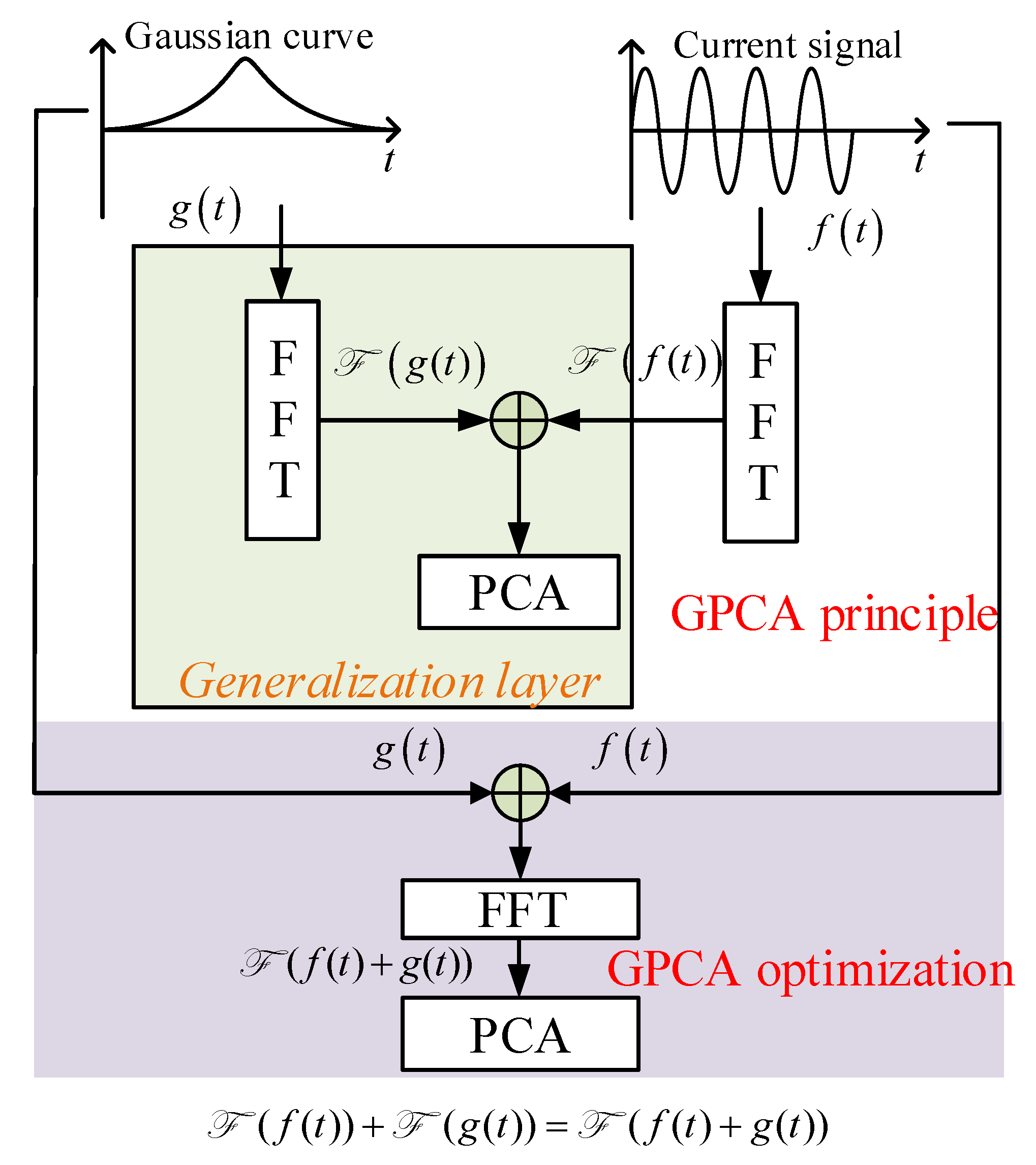
• This paper proposes the GPCA method, which addresses the issue of unreliable diagnostic results caused by singular matrix training sets by introducing a generalization layer.
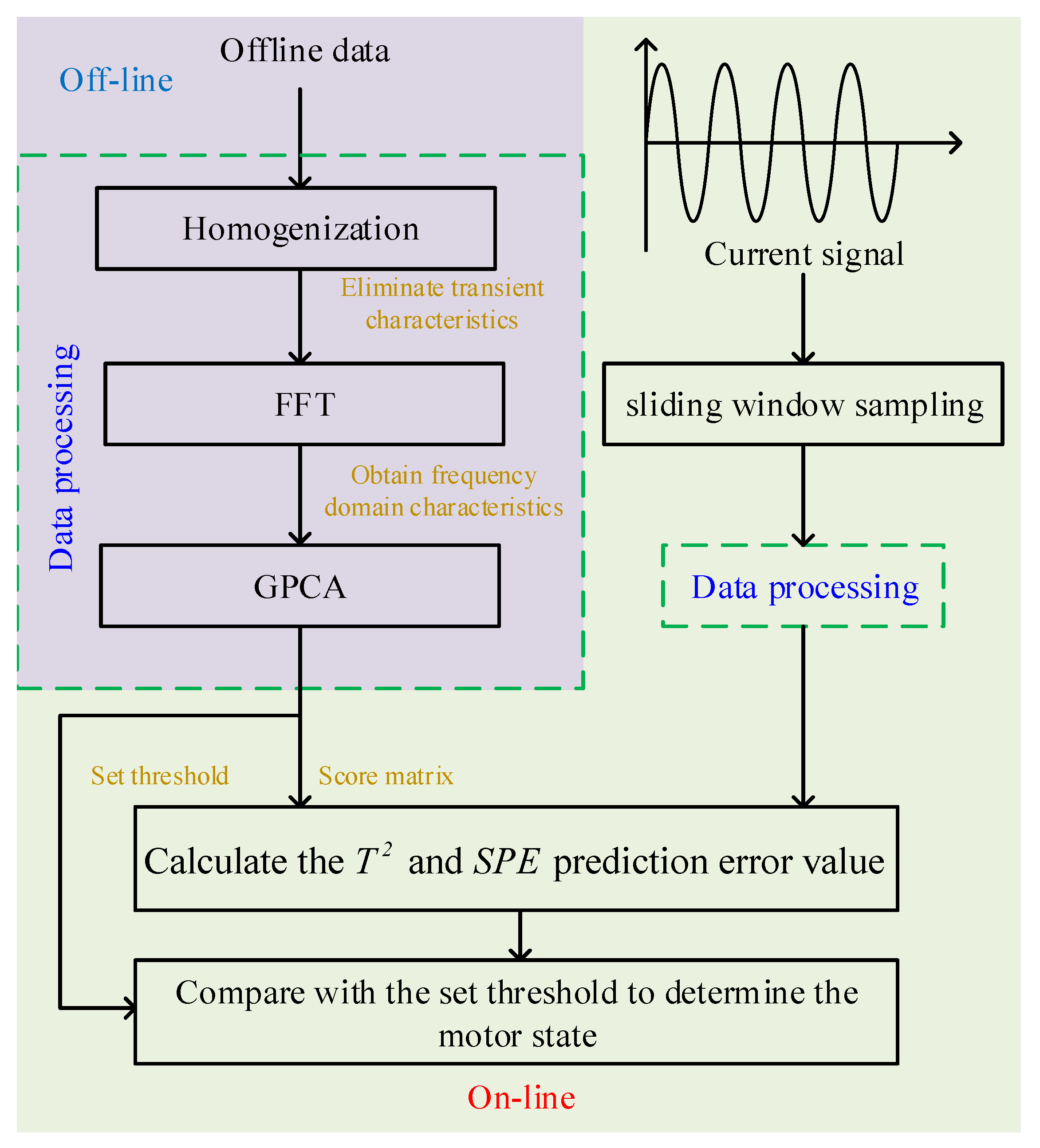
• This paper proposes a health status detection method for motor drive systems, including motor working status detection and the diagnosis of inverter faults in motor control.
• The method proposed in this paper only requires current data from the stable working states of the motor for offline training, enabling online health status detection of motor drive systems.

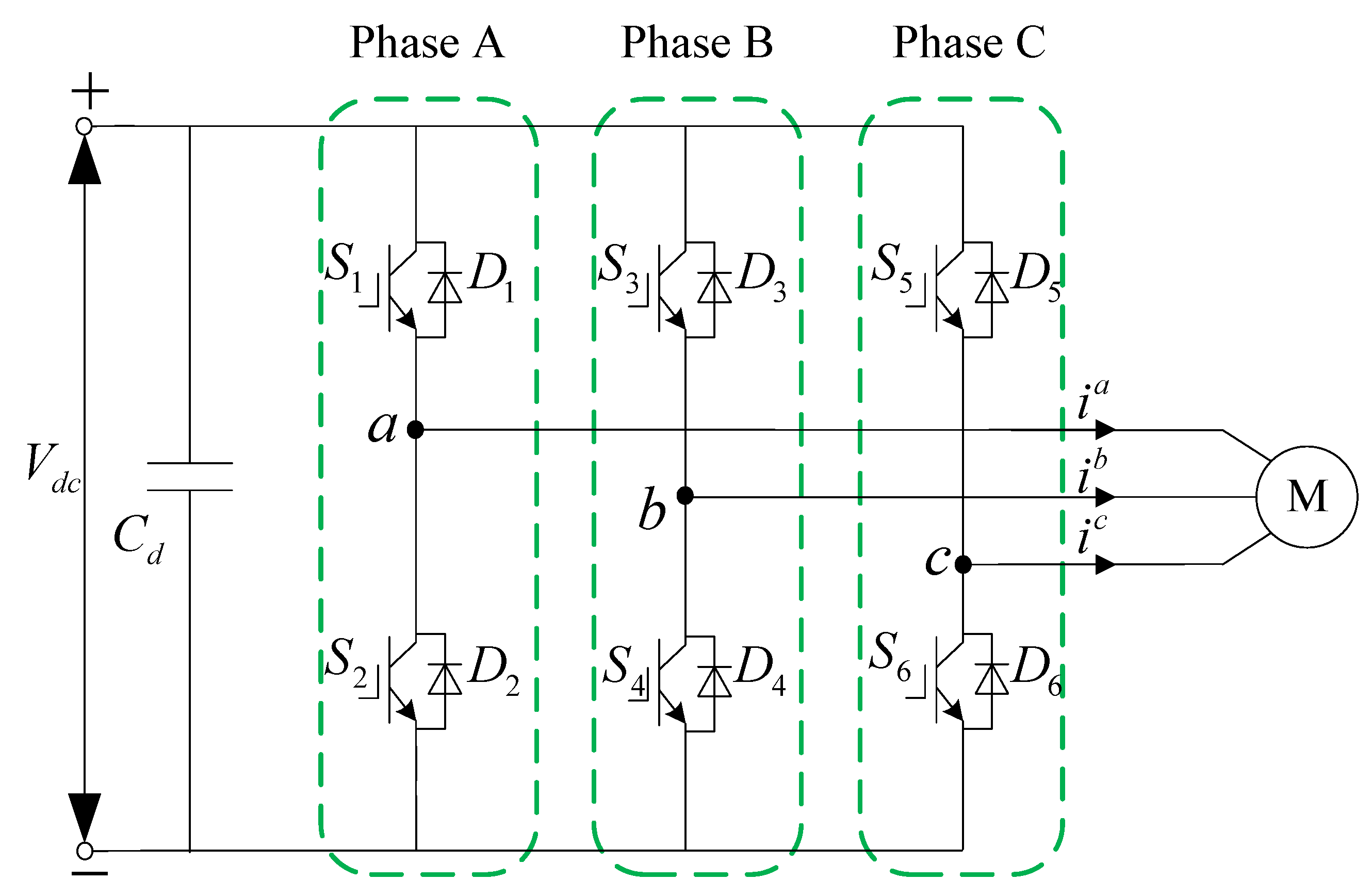
2. Topology and State Analysis of Power Circuits in Motor Drive Systems

2.1. Power Circuit Topology of a Motor Drive System

The topology of a two-level inverter is shown in Figure 1. The inverter is composed of six switching tubes ($S_1-S_6$) with anti-parallel diodes ($D_1-D_6$). $V_{dc}$ is the DC bus voltage [3]. $i^a$, $i^b$ and $i^c$ are three-phase currents. Their positive directions are indicated in Figure 1.

In many real-world applications, the load of a motor drive system undergoes real-time changes and is unpredictable [4]. The variability in load causes the entire drive system to frequently operate in transient processes [5]. In specific scenarios, such as changes in current due to a loading status or a load-shedding status, these variations can affect the diagnosis of the OC fault. Therefore, monitoring load changes hold guiding significance for the production process. The separation of the load-up state, the load-down state, and the OC fault state provides additional information that can be integrated into a manufacturing execution system (MES).

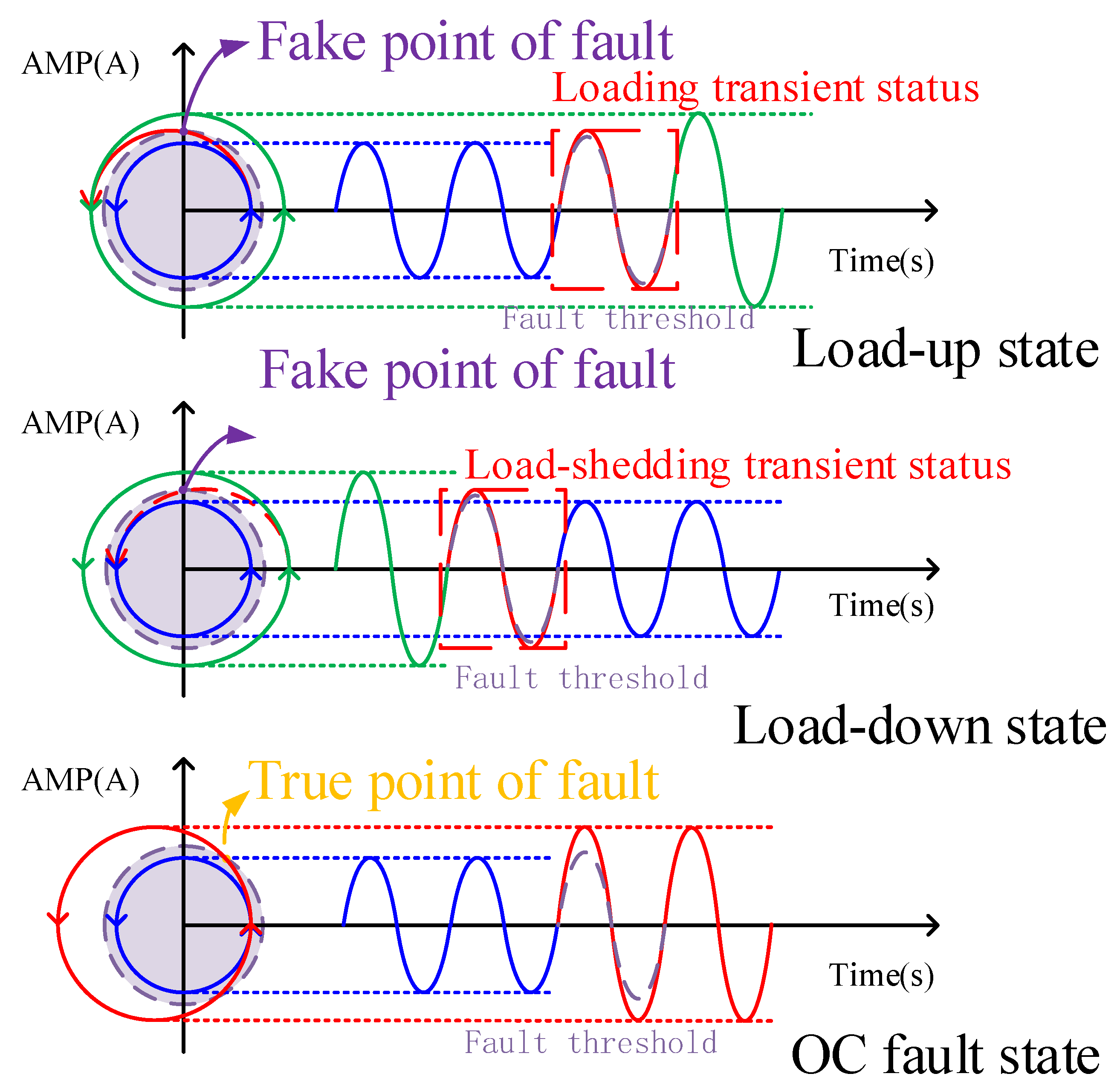
2.2. Load-Up/Load-Shedding Transient Process Analysis and Its Influence on Fault Diagnosis

Regardless of whether they are in the load-up state, the load-down state, or the OC fault state, the instantaneous currents still meet the requirements [6,8,9].

$$i^a+i^b+i^c=0.$$

(1)

When the switch tube of a certain phase has an OC fault, this phase current is distorted and the other two phase currents also vary due to (1). Three-phase currents are not symmetrical (see Figure 2) [7].

3. The Methodology for Health Status Detection for Motor Drive Systems

Since most current-based fault detection methods do not take into account transient currents during load changes, they exhibit poor resistance to interference. As shown in Figure 3, $I_0$ represents the current amplitude in the initial state, $I_1$ represents the current amplitude when transitioning to the second state, and $I_f$ represents the current amplitude after the fault occurs. During transient processes such as the loading/load-shedding state and the OC fault state, the instantaneous current value of the motor will change. It can be observed in Figure 3 that during the transient process of the loading/load-shedding state, the current vector will exceed the fault threshold. At this point, the above judgment method will mistakenly classify the loading/load-shedding state as an OC fault state.

During the transient processes of the loading/load-shedding status, the above method will mistakenly diagnose the loading/load-shedding state as a fault state due to the change in instantaneous current. The methods proposed in this article can address health status detection for motor drive systems.

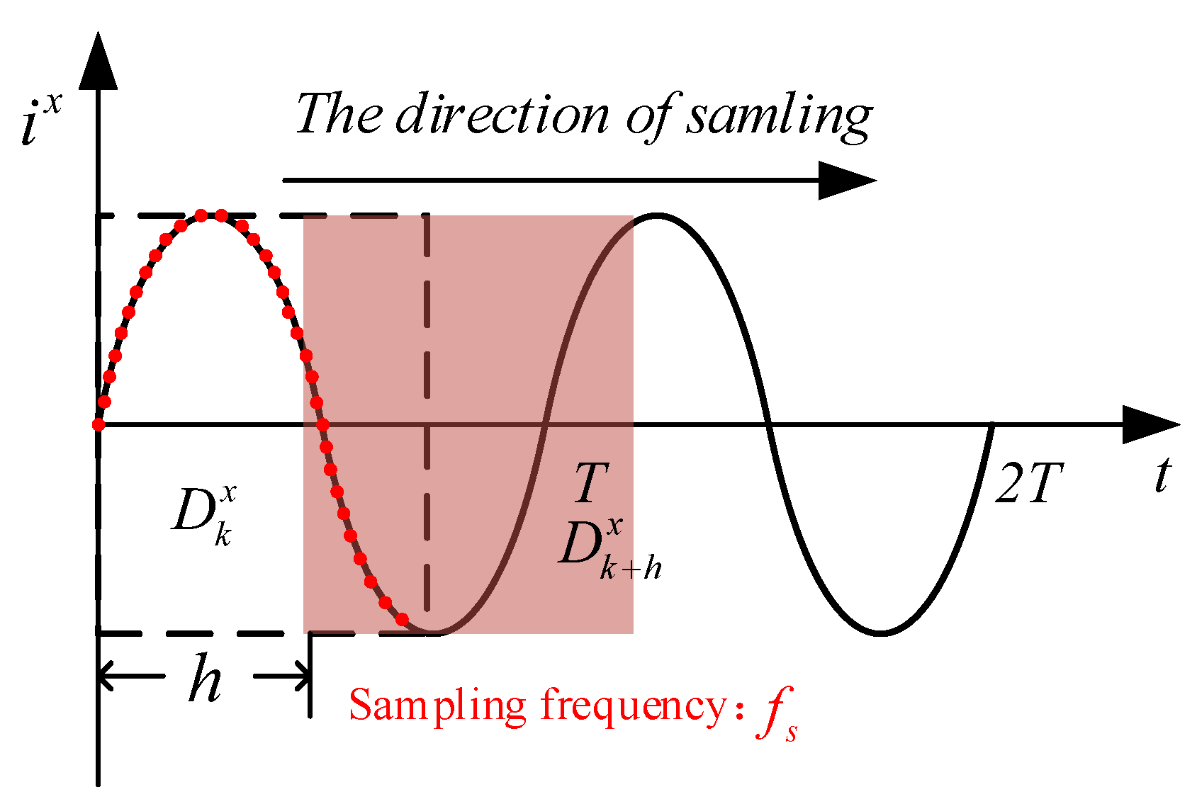
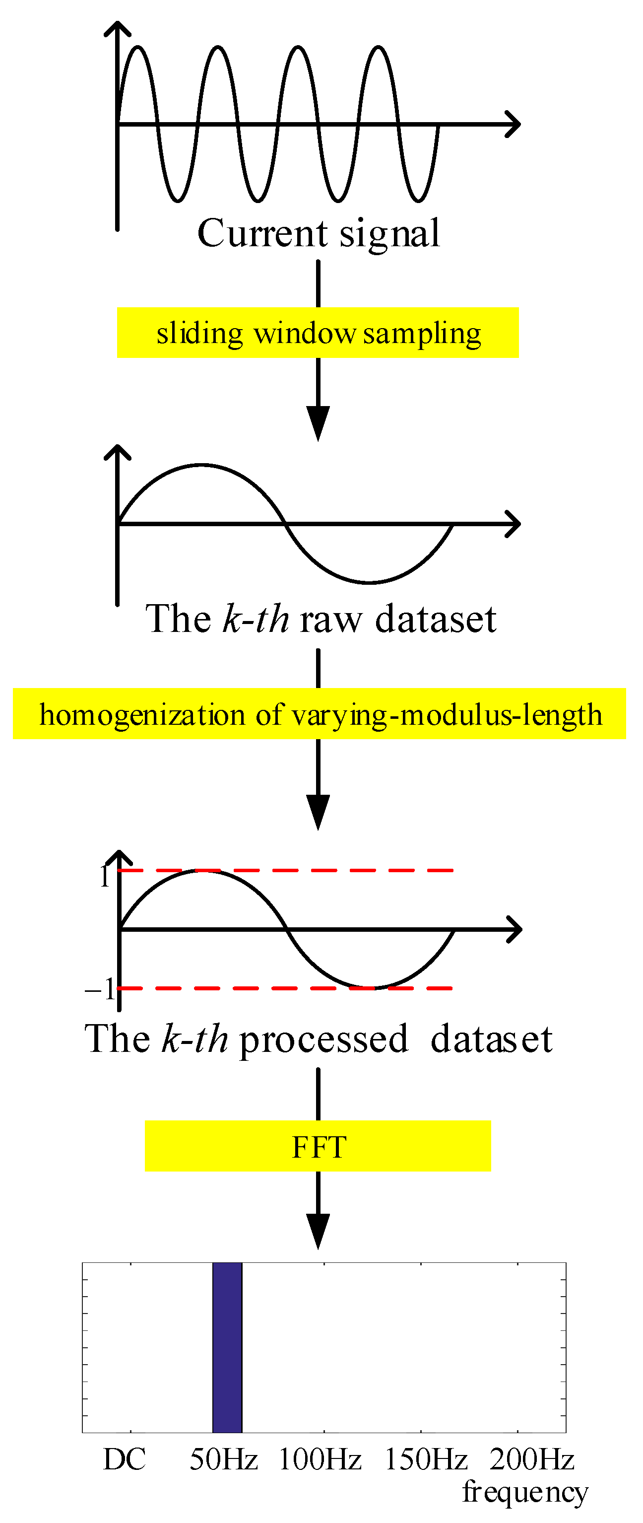
3.1. The Homogenization Process and Feature Extraction Using a Varying Modulus Length to Eliminate Transient Effects

This paper introduces a varying-modulus-length homogenization process to mitigate transient effects and employs the FFT for data feature extraction. The varying-modulus-length homogenization method utilizes the instantaneous current vector length to model the current waveform, identifying the actual cause of the current value change. This approach can effectively distinguish the transient effects associated with the loading/load-shedding states.

The input of the homogenization process is the current data sampled by the sliding window, and the output is the current data after modeling [9]. The length of the sliding window is N. The sliding step is h. k is the identifier of the set. The sampling frequency is $f_s$. $i_n^x$ is the instantaneous current value of phase x (x represents $a,b$ and c) at sampling point n, and the data set of the sliding window is

$$D_k^x=[i_{1+(k-1)h}^x,\dots ,i_{(k-1)h+N)}^x],k=1,2,\dots .$$

(2)

After length h, the next sliding window data set is

$$D_{k+1}^x=[i_{1+kh}^x,\dots ,i_{(k+1)h+N}^x],k=1,2,\dots .$$

(3)

The schematic diagram of the sliding window method is as follows (Figure 4).

The homogenization process is as follows. The sliding window sampling method collects the current data of phase a, phase b, and phase c, respectively. They are denoted as $D_k^a,D_k^b$ and $D_k^c$. The average error threshold $\epsilon$ is set to determine whether the current is a sine wave.

Step 1: The average value ${\overline{\mu }}_k^x$ of the three-phase currents is calculated at the sampling points in the sliding window N of the $k-th$ data set.

$${\overline{\mu }}_k^x=\frac{{\displaystyle \sum _{n=1+(k-1)h}^{(k-1)h+N}}{i}_n^x}{N},$$

(4)

where ${\overline{\mu }}_k^x$ represents the instantaneous value of the $k-th$ data set and $x=a,b$ and c.

Step 2: The calculated value ${\overline{\mu }}_k^x$ is compared with the error threshold $\epsilon$. If ${\overline{\mu }}_k^x<\epsilon$, it can be considered that the current waveform in the sliding window is a standard sine wave. The average error threshold requires that the current is also approximately regarded as a sine wave in the loading/load-shedding status. If ${\overline{\mu }}_k^x>\epsilon$, the three-phase current waveform is no longer a sine wave.

Step 3: If ${\overline{\mu }}_k^x<\epsilon$, a Clark transformation is performed on the three-phase current,

$$\left[\begin{array}{c}{i}_n^{\alpha }\\ i_n^{\beta }\end{array}\right]=\frac{2}{3}\left[\begin{array}{ccc}1& -\frac{1}{2}& -\frac{1}{2}\\ 0& \frac{\sqrt{3}}{2}& -\frac{\sqrt{3}}{2}\end{array}\right]\left[\begin{array}{c}{i}_n^a\\ i_n^b\\ i_n^c\end{array}\right],$$

(5)

where $i_n^a$, $i_n^b$ and $i_n^c$ represent the instantaneous value of the three-phase current at sampling point n and $i_n^{\alpha }$ and $i_n^{\beta }$ represent the current value at sampling point n after the coordinate changes.

Step 3.1: $i_n^{\alpha }$ and $i_n^{\beta }$ can be used to determine the instantaneous amplitude of the current, and then the following formula can be used to complete the homogenization process under normal operation and in the load-up state and load-shedding state.

$${\overline{i}}_n^x=\frac{i_n^x}{\sqrt{{\left(i_n^{\alpha }\right)}^2+{\left(i_n^{\beta }\right)}^2}},$$

(6)

where ${\overline{i}}_n^x$ is the processed data.

Step 3.2: The transformed ${\overline{i}}_n^x$ is reconstituted into a new data set after processing.

$${\overline{D}}_k^x=[{\overline{i}}_{1+(k-1)h}^x,\dots ,{\overline{i}}_{(k-1)h+N}^x].$$

(7)

Step 4: If ${\overline{\mu }}_k^x>\epsilon$, the current waveform is no longer regarded as a sine wave at this time. The data after homogenization using the above method will be distorted, so the following method is used to deal with this situation.

Step 4.1: First, the maximum value of the three-phase current is taken and marked as $i_{max}^x$.

$$i_{max}^x=max\left\{\left|D_k^x\right|\right\}.$$

(8)

Step 4.2: Next, the data in each data set are processed; the formula is as follows:

$${\overline{i}}_n^x=\frac{i_n^x}{i_{max}^x}.$$

(9)

Step 4.3: The transformed ${\overline{i}}_n^x$ is reconstituted into a new data set after processing, which is the same as the above Formula (7). The new data set formed contains the data after the normalization process, namely ${\overline{D}}_n^a,{\overline{D}}_n^b$ and ${\overline{D}}_n^c$.

The varying modulus length of the homogenization method is illustrated in Figure 5, where $I_0$ and $I_1$ represent the amplitudes of a specific phase current before and after a state change. The traditional method uses the maximum value in the sampling period as the denominator and the current value as the numerator. When processing current data using the traditional method, the current waveform tends to decrease during the transient processes of load-up or load-shedding. However, the homogenization method proposed in this paper effectively eliminates the influence of the loading/load-shedding transient states, thereby separating them from the OC fault state.

Figure 6 depicts the current waveform before homogenization, the current amplitude after applying the traditional normalization method, and the current amplitude following the homogenization method proposed in this article. The homogenization method introduced in this article effectively mitigates the impact of transient currents induced by load changes. The processed data allow for a better differentiation between the loading/load-shedding states and the OC fault state.

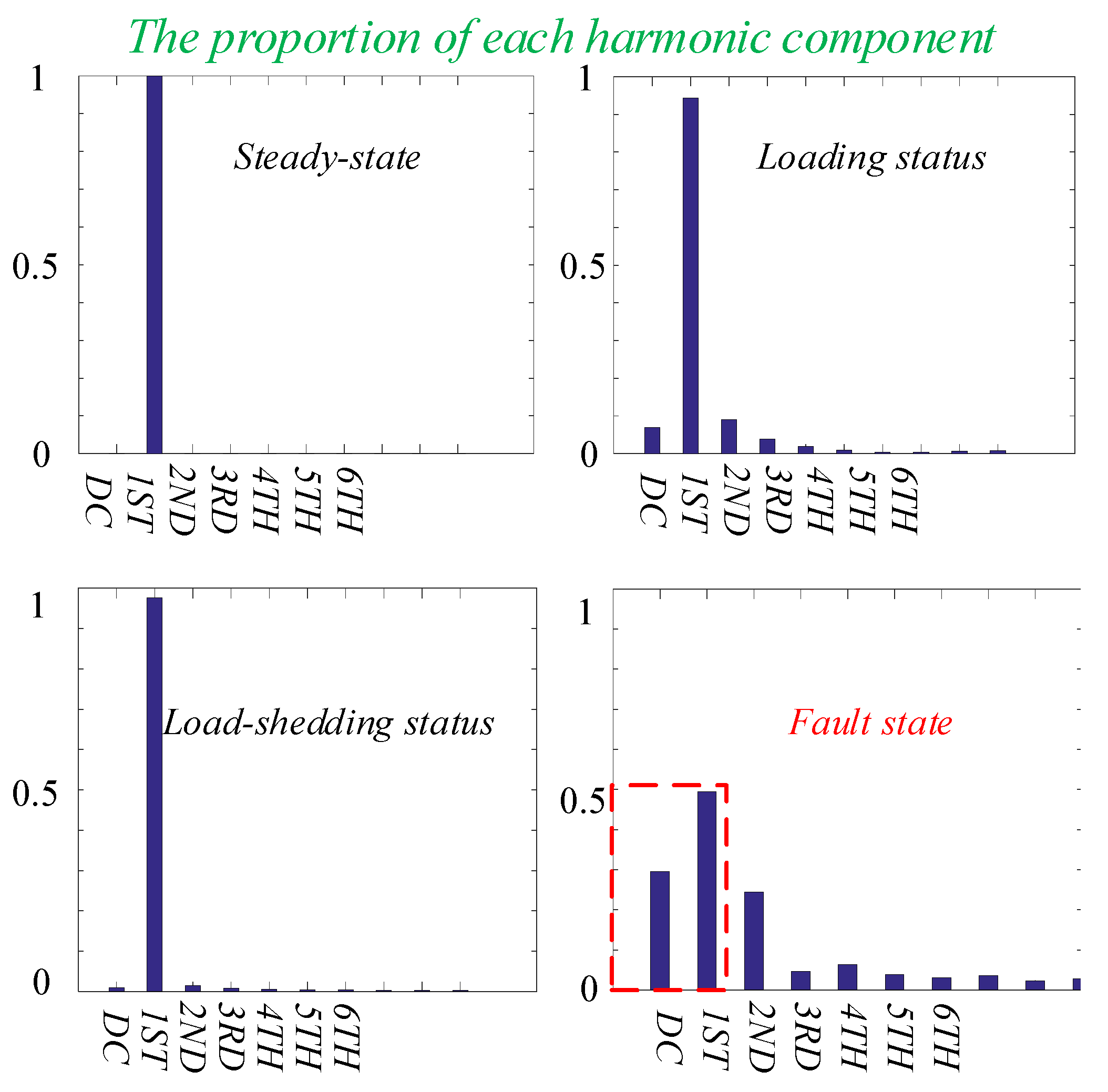
3.2. Feature Extraction Based on the FFT

By using the FFT to process the data set mentioned above, the components of the current waveform at different frequencies can be extracted [10]. In the stable state, the current after FFT processing contains only the fundamental wave component, and the amplitude of the fundamental wave component is equal to the current amplitude. When the system is in the loading/load-shedding state, the waveform after homogenization differs from the waveform in the steady state. After FFT processing, the components of each frequency change, with little variation in the fundamental wave component. In the OC fault state, the current amplitude undergoes significant distortion, and after FFT processing, each frequency component will be markedly different from the scenarios mentioned above. This is primarily reflected in a significant increase in the amplitude of the direct current (DC) component and a significant decrease in the amplitude of the fundamental component. Other harmonics also show an increase. The FFT results of current data in various states are shown in Figure 7.

FFT processing is performed on each ${\overline{D}}_k^x$ in the homogenization data set; the formula is

$$M=\left[\begin{array}{ccc}{m}_0^a& m_0^b& m_0^c\\ m_1^a& m_1^b& m_1^c\\ ⋮& ⋮& ⋮\\ m_n^a& m_n^b& m_n^c\end{array}\right]=F(\left[\begin{array}{c}{\overline{D}}_k^a\\ {\overline{D}}_k^b\\ {\overline{D}}_k^c\end{array}\right]),$$

(10)

where $m_0^x$ represents the DC component of phase x, $m_1^x$ represents the fundamental component of phase x, $m_n^x$ represents the $n-th$ harmonic component of phase x ($x=a,b$ and c), and F represents the FFT function. The data processing workflow of this paper is shown in Figure 8.

Through the methods of homogenization and the FFT, the transient effects of the loading/load-shedding states can be eliminated and the changes in current can be reduced. Consequently, the OC fault state can be effectively distinguished.

3.3. Motor Working State Detection and OC Fault Diagnosis of Inverters Based on GPCA

Aiming to improve the original shortcomings of PCA, we propose generalized layer-added PCA. The data after feature extraction are processed by GPCA, and the loading/load-shedding states can be separated through three indicators, including $T^2$, the $SPE$ prediction error, and contribution proportion. At the same time, fault diagnosis of the inverter can be accurately and quickly realized.

PCA is a multivariate statistical analysis method [19,20,21]. This article uses current data under the stable state as training data [13,15]. When PCA is used to detect the running status of the motor, the prediction error index of PCA is too high because the training matrix is not full rank. Figure 9 shows $T^2$ and $SPE$ of the motor by using the PCA method.

Such data are not credible. The reason why the prediction error value is so large is that the training matrix does not have a full rank. The specific analysis is as follows. When using the PCA method, the training matrix in a stable state must be normalized in the offline process.

$${\widehat{m}}_i^x=\frac{m_i^x-\overline{m}}{s},$$

(11)

where ${\widehat{m}}_i^x$ is the normalized value of the i-th harmonic of phase x, $\widehat{m}$ is the average value of the amplitude of each harmonic component, and s is the standard deviation of the amplitude of each harmonic component.

During steady-state operation, the amplitudes of the three-phase currents are equal, and the phase difference is 120°. After FFT processing, the amplitudes of the DC component, fundamental wave, and n-th harmonic component are approximately the same. This results in a singular training matrix. When processing the test matrix, the homogenization method is still performed using the average and standard deviation of the training matrix. At this time, $T^2$ and $SPE$ calculated by matrix M are excessively large, leading to unreliable data. Through the above analysis, the fundamental reason for the unreliable prediction error values is that the training matrix is not of full rank, indicating that $s\approx 0$.

This paper improves this situation by adding a generalized layer, which ensures that the condition number of the training matrix is greater than a certain constant $\delta$ (see Figure 10). The method after introducing the generalized layer is called GPCA. To enhance the credibility of the data set without affecting detection results, narrow Gaussian white noise is added. When selecting the Gaussian curve, it should be noted that the amplitude of the Gaussian white noise should not exceed $5\%$ of the current amplitude in the stable operating state. Taking a $5A$ current as an example, the amplitude of the external Gaussian white noise should be in the range of $[-0.025,0.025]$.

The following can be obtained by the linear property and signal superposition of the FFT:

$$F\left(f\right(t)+g(t\left)\right)=F\left(f\right(t\left)\right)+F\left(g\right(t\left)\right),$$

(12)

where $f\left(t\right)$ is the current signal and $g\left(t\right)$ is the input signal of the generalization layer. It can be observed from Formula (12) that the input signal of the generalization layer and the current signal undergo FFT processing and then are superimposed. This is equivalent to directly adding the input signal of the generalization layer to the current signal and subsequently applying FFT processing. This optimization adopts the latter method, where the generalization layer is added to the current signal and then the FFT is performed. This approach saves a significant amount of calculation time and enhances the sensitivity of inverter fault diagnosis.

The GPCA model decomposes the matrix after adding the generalization layer into

$$\widehat{M}=TVD=T\overline{P},$$

(13)

where the V matrix is a diagonal matrix composed of eigenvalues. The eigenvalues in the diagonal matrix V are arranged in descending order, and the product of the matrix $V^{\prime }$ and the matrix D in descending order is recorded as $\overline{P}$.

The first l term in matrix $V^{\prime }$ is chosen to remain unchanged as the principal element; remaining eigenvalues are all replaced by 0, without affecting the discrimination accuracy, to achieve the purpose of eliminating many interferences. The processed matrix $\widehat{M}$ is decomposed into

$$\widehat{M}=T{V}^{\prime }D=\sum _{j=1}^m{t}_j{p}_j^T+E=T{P}^T+E,$$

(14)

where the load matrix is $P\in R^{m\times l}$, which consists of l eigenvectors. The scoring matrix is $T\in R^{n\times l}$; each column of the scoring matrix T is called a principal variable, l represents the number of principals, and all columns of the scoring matrix T are orthogonal to each other. E is the residual space.

After obtaining the data sample, $SPE$ and $T^2$ can be used to detect whether a fault has occurred. $SPE$ measures the change in the projection of the sample vector in the residual space. ${\delta }^2$ represents the control limit of $SPE$ when the confidence level is $\alpha$. $T_{\alpha }^2$ represents the control limit of $T^2$ when the confidence level is $\alpha$. The calculation formulas of $SPE$ and $T^2$ are

$$SPE=\left|\right|I-{PP}^T\widehat{M}{\left|\right|}^2,$$

(15)

$$T^2={\widehat{M}}^{T}P{\Lambda }^{-1}{P}^T\widehat{M}.$$

(16)

The GPCA method has an added generalization layer to address the shortcomings of the PCA method. The results obtained by the GPCA method not only resist interference but also achieve fault diagnosis of an inverter by considering load changes. The results obtained by the GPCA method not only resist interference but also achieve health status detection of a motor drive system by considering load changes.

4. Results and Discussion

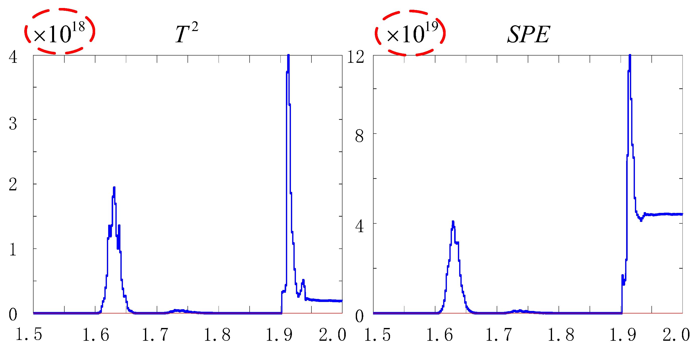
4.1. Motor Working State Detection

When feature extraction is performed on the data via the FFT, the DC component, fundamental wave, and various harmonic components in the transient process of the loading/load-shedding states are different. Although the current amplitude in the stable state is transformed into $[-1,1]$ after homogenization, the frequency of the current changes during the loading/load-shedding states. Assuming the motor is in a stable working state at this time, the speed is equal to a given value and the electromagnetic torque is equal to the load torque. That is, $\omega ={\omega }^{*}$ and $T=T_L$. The stator voltage frequency is ${\omega }_1=\omega +{\omega }_s$. During the loading transient, the load torque $T_L$ increases, causing the rotational speed $\omega$ to drop under the action of load torque, and the positive feedback inner loop makes ${\omega }_1$ drop. The load will elongate the inverter current cycle. Similarly, when in the load-shedding state, the inverter’s current cycle will become shorter. In the sliding window sampling process with a fixed step size, part of the current data for one cycle will be collected during loading. In the load-shedding state, part of the current data in the next cycle will be collected, as shown in Figure 11. Therefore, the components after the FFT are different, and the component of the transient process of the loading state is higher than the component of the transient process of the load-shedding state. GPCA makes the gap between the loading state and the load-shedding state more obvious. In the process of the loading/load-shedding state, for example, the diagonal matrix’s eigenvalues are arranged in descending order, so the calculation formula of $T^2$ can be simplified to

$$T^2=\sum _j^l{\lambda }_i{\alpha }_{ij}^2,$$

(17)

where ${\alpha }_{ij}$ is the element of the product of the current value of the test set and the training matrix. ${\lambda }_i$ is the one-dimensionality reduction sorting of the front one-dimensional principal elements of the diagonal matrix, which can be regarded as a weight function. During the transient process of the loading state, the front l-dimensional element undergoes significant changes. Similarly, during the transient process of the load-shedding state, the front l-dimensional element also changes, but these changes are much smaller than the element values observed during the loading state. After the squaring calculation, the gap becomes more pronounced. At this point, a threshold should be set for the GPCA prediction error value to distinguish between the motor’s loading state and load-shedding state. This threshold is referred to as the loading threshold. The selection of the loading threshold must meet a condition; namely, it should be smaller than the minimum value of $T^2$ and $SPE$ that can detect the minimum loading current. In this paper, load states below $1.25$ times the rated current are considered as fluctuations. Therefore, the loading threshold can be set to the maximum value of $T^2$ and $SPE$ during the transient process when the load is 1.25 times the rated current.

In summary, the GPCA method includes an offline process and an online process. The offline process mainly relies on historical data to determine the $SPE$ control limit ${\delta }^2$, $T^2$ control limit $T_{\alpha }^2$, loading thresholds ${\delta }_{\mathrm{upload}}^2$ and $T_{\mathrm{upload}}^2$, and fault thresholds ${\delta }_{\mathrm{fault}}^2$ and $T_{\mathrm{fault}}^2$. The online process only needs to calculate the prediction error values $SPE$ and $T^2$ and compare them with the threshold.

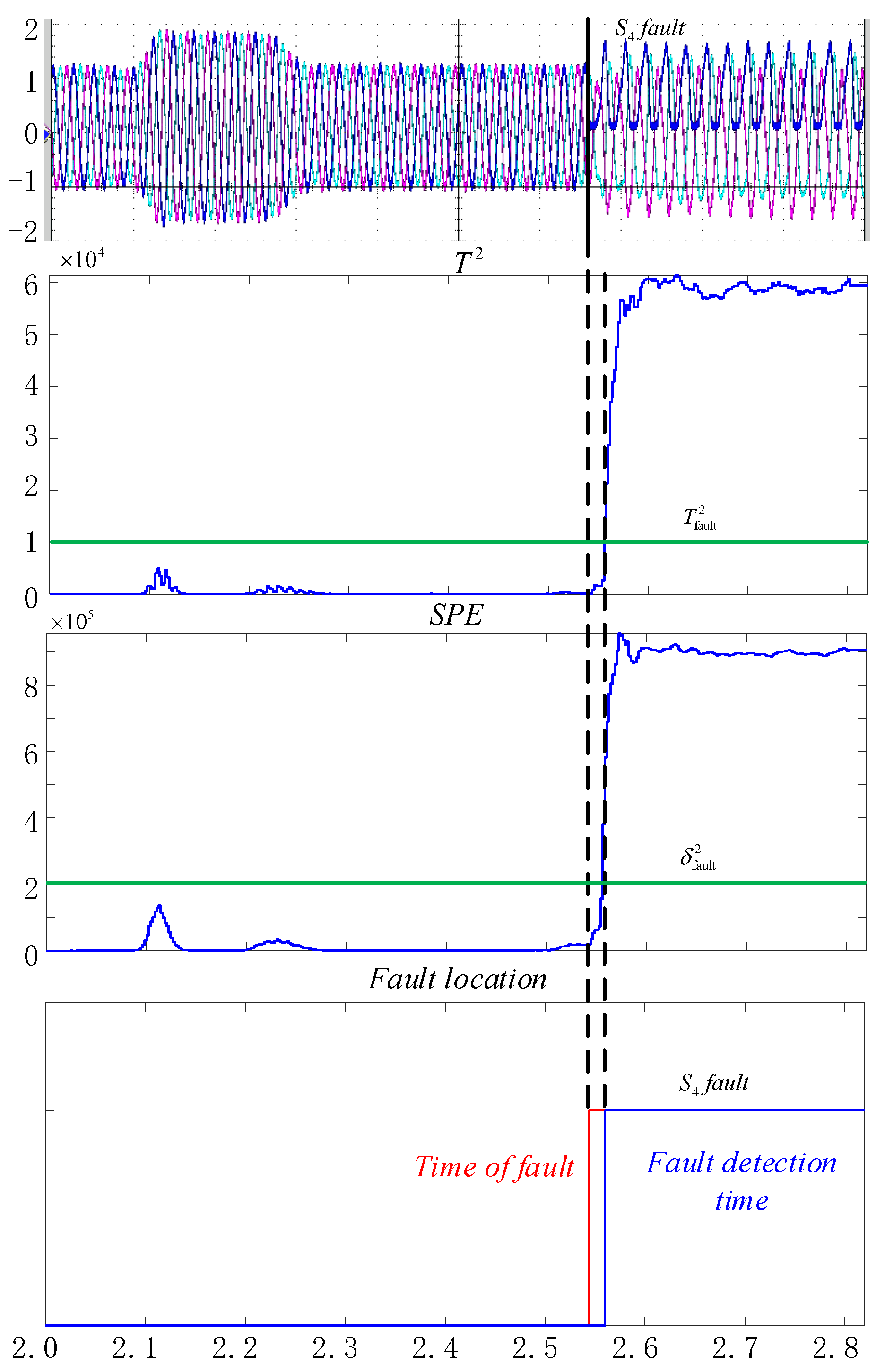
4.2. OC Fault Diagnosis of VSIs

In GPCA, the prediction error value and the fault threshold can be used to determine the whether an OC fault has occurred and the contribution proportion can be used to accurately locate the fault. When an OC fault occurs, the prediction error value calculated by the GPCA method after the data are normalized is large, while the loading/load-shedding state is very small. It can be judged whether the motor drive system is in the OC fault state by setting a threshold. Since $T^2$ and $SPE$ in the loading state are much smaller than $T^2$ and $SPE$ during the transient process of the fault state and the trend in $T^2$ and $SPE$ when a fault occurs is relatively simple, the setting of the fault threshold is crucial. To improve the speed of fault detection, the fault threshold is set equal to the prediction error value of $T^2$ and $SPE$ during the OC fault state. If $T^2$ and $SPE$ exceed the corresponding fault thresholds $\delta {\mathrm{fault}}^2$ and $T{\mathrm{fault}}^2$, it is considered that an OC fault has occurred at that time.

In the GPCA method, contribution proportions are used to locate fault components. Taking phase A as an example, Figure 12 and Figure 13 represent the contribution proportions of the three-phase current DC component and each harmonic when the switch tubes $S_1$ and $S_4$ have an OC fault. The first three terms in the figure represent the DC component contribution proportions of the three-phase currents $Q_{dc}^a$, $Q_{dc}^b$, and $Q_{dc}^c$, respectively. The fourth to sixth terms are the fundamental wave component contribution proportions of the three-phase currents $Q_{1st}^a$, $Q_{1st}^b$, and $Q_{1st}^c$. ${\eta }_{\mathrm{fault}}$ represents the fault threshold in the contribution proportion diagram. ${\eta }_{\mathrm{fault}}$ is used to compare the fundamental wave components of the currents in phases A, B, and C. When the fundamental wave component of a certain phase current exceeds the fault threshold, it can be considered that the switch tube controlling that phase current has an OC fault. As shown in Figure 12, when the fundamental wave contribution proportion of phase A exceeds the fault threshold ${\eta }_{\mathrm{fault}}$, it indicates that phase A has an OC fault. When the ratio of the DC component contribution proportion of phase A to its fundamental wave contribution proportion is less than the constant 0.5, it indicates the switch tubes $S_1$ have an OC fault. Similarly, in Figure 13, when the ratio of the DC component contribution proportion of phase A to its fundamental wave contribution proportion is greater than the constant 0.5, it indicates the switch tubes $S_4$ have an OC fault.

As shown in Figure 14, when the switch tube $S_1$ has an OC fault, the forward current in phase A will instantaneously disappear. Consequently, the DC component of phase A exhibits minimal changes during the FFT, while the fundamental wave component undergoes significant changes. Therefore, the ratio of $Q_{dc}^a$ to $Q_{1st}^a$ is small. When the switch tube $S_4$ experiences an OC fault, the negative current in phase A will instantaneously disappear, but the positive current in the next cycle will still exist. Hence, $Q_{dc}^a$ undergoes significant changes during the FFT, while the fundamental component undergoes minimal changes, resulting in a large ratio of $Q_{dc}^a$ to $Q_{1st}^a$. Using 0.5 as the limit of the ratio helps determine which switch tube has an OC fault. As shown in Figure 12, the amplitude of the DC component is significantly higher when switch tube $S_1$ has an OC fault compared to when switch tube $S_4$ has an OC fault. The amplitude of the fundamental wave component is significantly lower when switch tube $S_1$ has an OC fault compared to when switch tube $S_4$ has an OC fault. However, regardless of whether $S_1$ or $S_4$ has an OC fault, the fundamental component of the phase A current undergoes the most significant change, and it will exceed the threshold ${\eta }_{\mathrm{fault}}$ when calculating the contribution proportion $Q^a$.

Suppose the corresponding values of A, B, and C are 1, 2, and 3, respectively, when a fault occurs, and the value is recorded as 0 when there is no fault. The fault value is defined as $F_{\mathrm{indication}}$.

$$F_{\mathrm{indicator}}=\left\{\begin{array}{cc}0,\hfill & Q_{1\mathrm{st}}^x<{\eta }_{\mathrm{fault}}\hfill \\ 1,\hfill & Q_{1\mathrm{st}}^a>{\eta }_{\mathrm{fault}}\hfill \\ 2,\hfill & Q_{1\mathrm{st}}^b>{\eta }_{\mathrm{fault}}\hfill \\ 3,\hfill & Q_{1\mathrm{st}}^c>{\eta }_{\mathrm{fault}}\hfill \end{array}\right.,$$

(18)

where $Q_{\mathrm{dc}}^x$ represents the fundamental component in phase x and $x=a,b$ and c.

After determining the fault phase, the fault switch tube is located. When a fault occurs, the ratio of the DC component contribution proportion of the fault item to the fundamental wave contribution proportion is distinctly different. When $S_1$ has an OC fault, the ratio is less than 0.5, and when $S_4$ has an OC fault, the ratio is more than 0.5. In summary, Equation (19) can be used to calculate the values corresponding to different switch tube faults.

$$F=\mathrm{Round}(\frac{Q_{\mathrm{dc}}^x}{Q_{1\mathrm{st}}^x}+0.5)\times 10+F_{\mathrm{indicator}},$$

(19)

where F represents the fault value of the switch tube and $\mathrm{Round}(\dot{)}$ is the rounded up function. $Q_{\mathrm{DC}}^x$ and $Q_{1\mathrm{st}}^x$ are the DC component and fundamental wave component of the fault phase, respectively. At this time, the position of the switch tube where the fault occurred can be located according to the look-up table (

Table 2. Fault location look-up table.

Fault Phase	Fault Switch Tube	Fault Value F
phase A	$S_1$	21
	$S_4$	11
phase B	$S_3$	22
	$S_6$	12
phase C	$S_5$	23
	$S_2$	13

).

The overall process of health status detection is illustrated in Figure 15. The method in this paper is divided into two processes: the offline process (Off-line) and the online process (On-line). In the offline process, data are processed using the homogenization method and then data features are extracted using the FFT. The multi-dimensional features are fed into the GPCA algorithm model to calculate the control limit ${\delta }^2$ of $SPE$ and the control limit $T_{\alpha }^2$ of $T^2$. Simultaneously, parameters ${\delta }_{\mathrm{upload}}^2$, $T_{\mathrm{upload}}^2$, ${\delta }_{\mathrm{fault}}^2$, and $T{\mathrm{fault}}^2$ are set. In the online process, after data processing, only the values of $SPE$ and $T^2$ need to be calculated and compared with the pre-set ${\delta }^2$, $T{\alpha }^2$, ${\delta }_{\mathrm{upload}}^2$, $T_{\mathrm{upload}}^2$, ${\delta }_{\mathrm{fault}}^2$, and $T_{\mathrm{fault}}^2$ from the previous offline process training. When the fault threshold is exceeded, the contribution proportion is calculated, and the fault value F is used to locate the fault.

The GPCA method solves the problem of the PCA method misjudging the normal loading/load-shedding process as a fault state due to load fluctuations. GPCA retains the advantage of the PCA method of a short diagnosis time and also realizes fault location.

Table 3. Comparison of various methods.

Diagnosis Method	Time	Loading and Load-Shedding Status	Fault Location
GPCA	$0.5T$	yes	yes
PCA [21]	$0.5T$	no	no
Current deviation method	$2.0T$	no	yes

shows a comparison between GPCA and other methods.

4.3. Simulation and Experiment

PLECS 4.6.2 simulation software was used to build a simulation model, as shown in Figure 1. The load is an asynchronous motor. The given bus voltage of the system is $538\mathrm{V}$, and the rated current of the motor is $4\mathrm{A}$. The specified fault phase of the simulation is phase A, and the motor’s working state includes a loading state, a load-shedding state, and an inverter OC fault state.

During the simulation process, the current sampling frequency is $25\mathrm{kHz}$, $N=500$, and the sliding window period is $20\mathrm{ms}$. The motor load-up state is set at $1.7\mathrm{s}$ and $2\mathrm{s}$, the motor load-down state is set at $1.8\mathrm{s}$ and $2.2\mathrm{s}$, and the inverter OC fault state is set at $2.4\mathrm{s}$ during the motor operation.

Figure 16 depicts the simulation results of health status detection for a motor drive system, including motor state detection and inverter fault diagnosis. By comparing the loading threshold and the fault threshold, the working state of the motor can be accurately determined, and simultaneously, the position of the faulty inverter switch tube can be located, as shown in Figure 17. The fault value F of the faulty switch tube is calculated based on the contribution proportion to determine the fault location. The methodology of this paper has been validated through simulations, demonstrating its capability to achieve health status detection for motor drive systems.

In an asynchronous motor empty-load experiment, we conducted tests involving a loading state and a load-shedding state to an empty load and simulating an OC fault. We modelled an OC fault by disconnecting the control signal of the switching tube. The empty-load current is $1\mathrm{A}$ and the OC fault occurs in the down tube corresponding to phase A, i.e., $S_4$ contains the OC fault. Figure 18 displays the experimental platform. The variation in load does not present an ideal step function, but this does not affect the experimental results.

Figure 19 presents the experimental results, corresponding to the three-phase current waveforms sampled in the oscilloscope, the respective prediction error values, and the fault location diagram. In the fault location diagram, blue represents the time when the fault occurred and red represents the actual time when the fault occurred. The time difference between the two is approximately $0.5\mathrm{T}$. The experimental results demonstrate that the methodology proposed in this paper can achieve health status detection for motor drive systems. The methodology can utilize current data from healthy operating conditions as an offline data set, which are easily accessible.

5. Conclusions

The methodology proposed in this paper realizes health status detection for motor drive systems. This approach can detect the motor working status as well as diagnose an open-circuit (OC) fault in the inverter. The proposed GPCA method overcomes the limitation of the PCA method in handling data when facing singular matrices. By introducing a generalized layer, the GPCA method can train with singular matrices, thus addressing the issue of misjudging the loading transient state and load-shedding transient state as fault states. This method can train the model offline using only healthy data and achieve online motor drive system health status detection. It exhibits strong anti-interference capabilities, performing well in environments with frequent load changes and multiple interferences. This paper focuses on health status detection for motor drive systems, particularly addressing open-circuit faults in the inverter. Our assumption is based on using the GPCA method to handle data, which effectively deals with situations involving singular matrices. Potential future works include further improvement and optimization of the GPCA method to enhance its performance under different working conditions, as well as extending its application to other fields such as industrial control systems and smart manufacturing.

References

1. Song, Y.; Zhao, J. Model Predictive Flux Control-Based Open-Circuit Fault Diagnosis Method for Two-Level Three-Phase Inverter Induction Motor Drive. In Proceedings of the 2022 41st Chinese Control Conference (CCC), Hefei, China, 25–27 July 2022; pp. 3912–3916. [Google Scholar]
2. Manikandan, R.; Raja Singh, R. Fault diagnosis of wind turbine power converter using intrinsic mode functions with relative energy entropy. Circuit World 2024, 50, 90–107. [Google Scholar]
3. Manikandan, R.; Raja Singh, R. Robust Open-Circuit Fault Diagnosis of Multi-Phase Floating Interleaved DC–DC Boost Converter Based on Sliding Mode Observer. IEEE Trans. Transp. Electrif. 2019, 5, 638–649. [Google Scholar]
4. Zhou, Y.; Zhao, J.; Song, Y.; Sun, J.; Fu, H.; Chu, M. A Seasonal-Trend Decomposition Based Voltage-Source-Inverter Open-Circuit Fault Diagnosis Method. IEEE Trans. Ind. Electron. 2022, 37, 15517–15527. [Google Scholar] [CrossRef]
5. Seninete, S.; Abed1, M.; Bendiabdellah, A.; Mimi, M.; Belouchrani, A.; Ali, A.O.; Cherif, B.D.E. On the use of high-resolution time-frequency distribution based on a polynomial compact support kernel for fault detection in a two-level inverter. Period. Polytech. Electr. Eng. Comput. Sci. 2020, 64, 352–365. [Google Scholar] [CrossRef]
6. Manikandan, R.; Raghu, S.; Singh, R.R. An Improved Open Switch Fault Diagnosis Strategy for Variable Speed Drives. In Proceedings of the 2022 IEEE International Conference on Power Electronics, Smart Grid, and Renewable Energy (PESGRE), Trivandrum, India, 2–5 January 2022. [Google Scholar]
7. Sahin, I.; Keysan, O. Model Predictive Controller Utilized as an Observer for Inter-Turn Short Circuit Detection in Induction Motors. IEEE Trans. Energy Convers. 2021, 36, 1449–1458. [Google Scholar] [CrossRef]
8. Rajeswaran, N.; Thangaraj, R.; Mihet-Popa, L.; Krishna Vajjala, K.V.; Özer, Ö. FPGA implementation of AI-based inverter IGBT open circuit fault diagnosis of induction motor drives. Micromachines 2022, 13, 663. [Google Scholar] [CrossRef] [PubMed]
9. Sun, X.; Diao, N.; Song, C.; Qiu, Y.; Zhao, X. An Open-Circuit Fault Diagnosis Method Based on Adjacent Trend Line Relationship of Current Vector Trajectory for Motor Drive Inverter. Machines 2023, 11, 928. [Google Scholar] [CrossRef]
10. Yan, H.; Xu, Y.; Zou, J.; Fang, Y.; Cai, F. A novel open-circuit fault diagnosis method for voltage source inverters with a single current sensor. IEEE Trans. Power Electron. 2017, 33, 8775–8786. [Google Scholar] [CrossRef]
11. Liang, Y.; Wang, R.; Hu, B. Single-Switch Open-Circuit Diagnosis Method Based on Average Voltage Vector for Three-Level T-Type Inverter. IEEE Trans. Power Electron. 2021, 36, 911–921. [Google Scholar] [CrossRef]
12. Xia, Y.; Xu, Y. A Transferrable Data-Driven Method for IGBT Open-Circuit Fault Diagnosis in Three-Phase Inverters. IEEE Trans. Power Electron. 2021, 36, 13478–13488. [Google Scholar] [CrossRef]
13. Gou, B.; Xu, Y.; Xia, Y.; Deng, Q.; Ge, X. An Online Data-Driven Method for Simultaneous Diagnosis of IGBT and Current Sensor Fault of Three-Phase PWM Inverter in Induction Motor Drives. IEEE Trans. Power Electron. 2020, 35, 13281–13294. [Google Scholar] [CrossRef]
14. Cherif, B.D.E.; Seninete, S.; Defdaf, M.; Berrabah, F. Diagnosis of Three-Phase Two-Level Voltage Inverter Under Open-Circuit Fault of an IGBT. In Artificial Intelligence and Heuristics for Smart Energy Efficiency in Smart Cities; Lecture Notes in Networks and Systems; Springer: Cham, Switzerland, 2022; pp. 674–681. [Google Scholar]
15. Cherif, B.D.E.; Bendiabdellah, A.; Bendjebbar, M.; Tamer, A. Neural network based fault diagnosis of three phase inverter fed vector control induction motor. Period. Polytech. Electr. Eng. Comput. Sci. 2019, 63, 295–395. [Google Scholar] [CrossRef]
16. Gmati, B.; Jlassi, I.; Khojet El Khil, S.; Marques Cardoso, A.J. Open-switch fault diagnosis in voltage source inverters of PMSM drives using predictive current errors and fuzzy logic approach. IET Power Electron. 2021, 14, 1059–1072. [Google Scholar] [CrossRef]
17. Cherif, B.D.E.; Chouai, M.; Seninete, S.; Bendiabdellah, A. Machine-Learning-Based Diagnosis of an Inverter-Fed Induction Motor. IEEE Lat. Am. Trans. 2022, 20, 901–911. [Google Scholar] [CrossRef]
18. Lee, H.-W.; Lee, K.-B. Open-Circuit Fault Diagnosis and Fault-Tolerant Operation of Dual Inverter for Open-End Winding Interior Permanent Magnet Synchronous Motor. In Proceedings of the 2022 IEEE 5th Student Conference on Electric Machines and Systems (SCEMS), Busan, Republic of Korea, 24–26 November 2022. [Google Scholar]
19. Zhang, X.; Ren, X. Two Dimensional Principal Component Analysis based Independent Component Analysis for face recognition. In Proceedings of the 2011 International Conference on Multimedia Technology, Hangzhou, China, 26–28 July 2011; pp. 934–936. [Google Scholar]
20. Pei, Y. Linear Principal Component Discriminant Analysis. In Proceedings of the 2015 IEEE International Conference on Systems, Man, and Cybernetics, Hong Kong, China, 9–12 October 2015; pp. 2108–2113. [Google Scholar]
21. Martins, J.F.; Pires, V.F.; Lima, C.; Pires, A.J. Fault detection and diagnosis of grid-connected power inverters using PCA and current mean value. In Proceedings of the IECON 2012—38th Annual Conference on IEEE Industrial Electronics Society, Montreal, QC, Canada, 25–28 October 2012; pp. 5185–5190. [Google Scholar]
Figure 1. Two-level inverter [9].
Mathematics 12 01690 g001
Figure 2. Three-phase currents during the loading/load-shedding state and OC fault [6].
Mathematics 12 01690 g002
Figure 3. Comparison of the current in the transient process of the motor.
Mathematics 12 01690 g003
Figure 4. Illustration of sliding window sampling [9].
Mathematics 12 01690 g004
Figure 5. Principle of homogenization of varying modulus length [9].
Mathematics 12 01690 g005
Figure 6. Current before and after homogenization.
Mathematics 12 01690 g006
Figure 7. FFT results of the loading/load-shedding states and the OC fault state.
Mathematics 12 01690 g007
Figure 8. Data processing.
Mathematics 12 01690 g008
Figure 9. T 2 and S P E prediction error of a motor by using the PCA method.
Mathematics 12 01690 g009
Figure 10. Principle and optimization of GPCA.
Mathematics 12 01690 g010
Figure 11. Cycle change and FFT result in loading/load-shedding states.
Mathematics 12 01690 g011
Figure 12. Contribution proportion when an S 1 fault occurs.
Mathematics 12 01690 g012
Figure 13. Contribution proportion when an S 4 fault occurs.
Mathematics 12 01690 g013
Figure 14. FFT results for the OC fault state of S 1 and S 4 .
Mathematics 12 01690 g014
Figure 15. The overall process of health status detection.
Mathematics 12 01690 g015
Figure 16. Simulation results of health status detection for a motor drive system.
Mathematics 12 01690 g016
Figure 17. Location of the faulty switch tube.
Mathematics 12 01690 g017
Figure 18. Experimental platform.
Mathematics 12 01690 g018
Figure 19. Experimental results.
Mathematics 12 01690 g019