
Imbalanced Data Classification Based on Improved Random-SMOTE and Feature Standard Deviation


Abstract
1. Introduction
- A new strategy based on feature standard deviation is proposed to detect the locations of samples. Feature standard deviation strategy utilizes standard deviation in feature dimensions among different samples to construct a boundary sample set, aiming to optimize the position of the decision boundary.
- An improved three-point interpolation method proposed in Random-SMOTE is presented to synthesize samples, where both inter-class and intra-class attributes are taken into account, with the purpose of avoiding overfitting and optimizing the decision boundary.
- A new method (FSDR-SMOTE) is proposed to deal with imbalanced data. The FSDR-SMOTE can enhance the diversity of synthetic samples in the minority class, reduce the probability of generating noisy samples, and improve the classification performance of the classifier.
2. Related Work
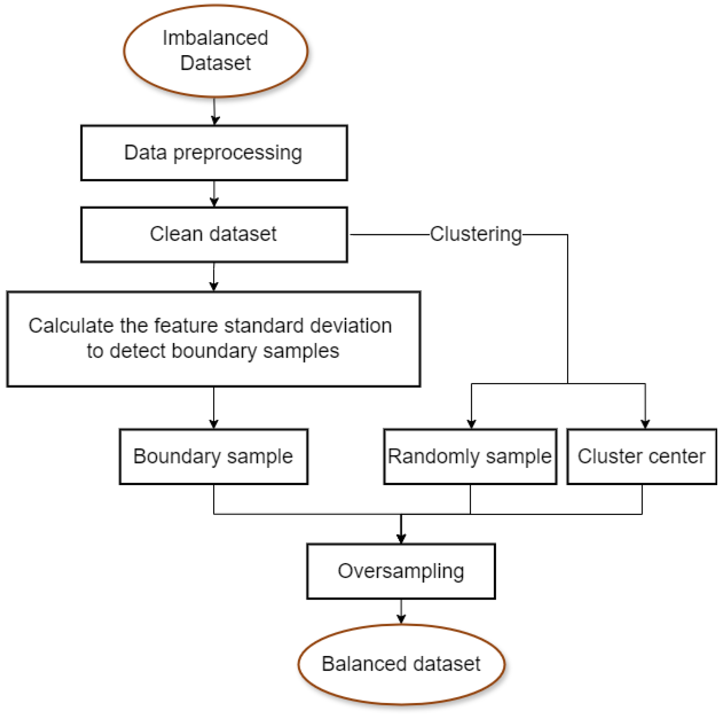
3. Method
| Algorithm 1 FSDR-SMOTE |
|
3.1. Data Preprocessing
3.2. Boundary Sample Screening
3.3. Synthesis of New Samples
4. Experimental Results and Analysis
4.1. Benchmark Dataset
4.2. Evaluation Indicator
4.3. Experimental Setup and Environment
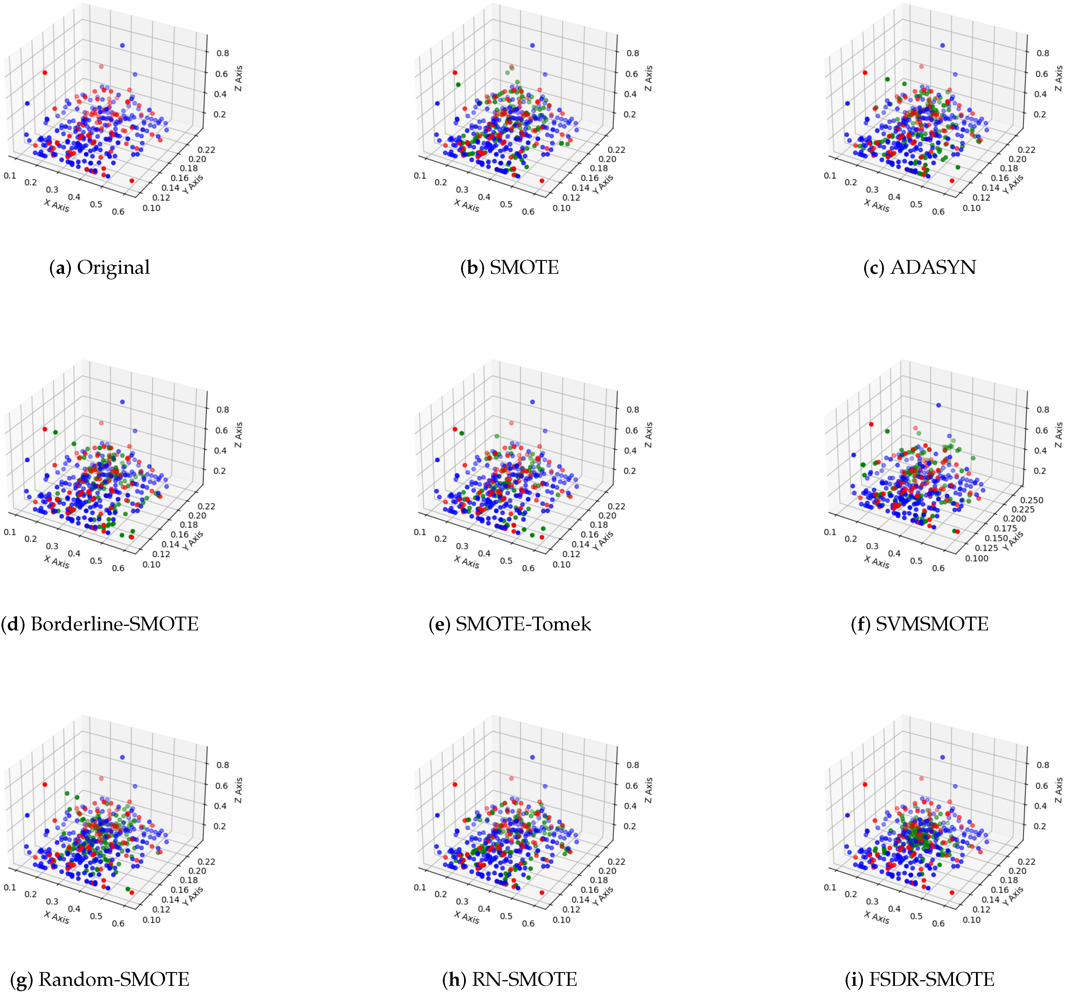
4.4. Comparison of Sampling Effects of Different Methods
4.5. Experimental Results
4.6. Ablation Study
5. Discussion
6. Conclusions
Author Contributions
Funding
Data Availability Statement
Conflicts of Interest
References
- Tomašev, N.; Mladenić, D. Class imbalance and the curse of minority hubs. Knowl. Based Syst. 2013, 53, 157–172. [Google Scholar] [CrossRef]
- Vasighizaker, A.; Jalili, S. C-PUGP: A cluster-based positive unlabeled learning method for disease gene prediction and prioritization. Comput. Biol. Chem. 2018, 76, 23–31. [Google Scholar] [CrossRef] [PubMed]
- Jurgovsky, J.; Granitzer, M.; Ziegler, K.; Calabretto, S.; Portier, P.E.; He-Guelton, L.; Caelen, O. Sequence classification for credit-card fraud detection. Expert Syst. Appl. 2018, 100, 234–245. [Google Scholar] [CrossRef]
- Malhotra, R.; Kamal, S. An empirical study to investigate oversampling methods for improving software defect prediction using imbalanced data. Neurocomputing 2019, 343, 120–140. [Google Scholar] [CrossRef]
- Zhou, X.; Hu, Y.; Liang, W.; Ma, J.; Jin, Q. Variational LSTM enhanced anomaly detection for industrial big data. IEEE Trans. Ind. Inform. 2020, 17, 3469–3477. [Google Scholar] [CrossRef]
- Tao, X.; Li, Q.; Guo, W.; Ren, C.; Li, C.; Liu, R.; Zou, J. Self-adaptive cost weights-based support vector machine cost-sensitive ensemble for imbalanced data classification. Inf. Sci. 2019, 487, 31–56. [Google Scholar] [CrossRef]
- Daneshfar, F.; Aghajani, M.J. Enhanced text classification through an improved discrete laying chicken algorithm. Expert Syst. 2024, e13553. [Google Scholar] [CrossRef]
- Revathy, V.; Pillai, A.S.; Daneshfar, F. LyEmoBERT: Classification of lyrics’ emotion and recommendation using a pre-trained model. Procedia Comput. Sci. 2023, 218, 1196–1208. [Google Scholar] [CrossRef]
- Chawla, N.V.; Bowyer, K.W.; Hall, L.O.; Kegelmeyer, W.P. SMOTE: Synthetic minority over-sampling technique. J. Artif. Intell. Res. 2002, 16, 321–357. [Google Scholar] [CrossRef]
- Nadi, A.A.; Gildeh, B.S.; Kazempoor, J.; Tran, K.D.; Tran, K.P. Cost-effective optimization strategies and sampling plan for Weibull quantiles under type-II censoring. Appl. Math. Model. 2023, 116, 16–31. [Google Scholar] [CrossRef]
- Tao, X.; Chen, W.; Li, X.; Zhang, X.; Li, Y.; Guo, J. The ensemble of density-sensitive SVDD classifier based on maximum soft margin for imbalanced datasets. Knowl. Based Syst. 2021, 219, 106897. [Google Scholar] [CrossRef]
- Li, W.; Sun, S.; Zhang, S.; Zhang, H.; Shi, Y. Cost-Sensitive Approach to Improve the HTTP Traffic Detection Performance on Imbalanced Data. Secur. Commun. Netw. 2021, 2021, 6674325. [Google Scholar] [CrossRef]
- Li, J.; Zhu, Q. A boosting self-training framework based on instance generation with natural neighbors for K nearest neighbor. Appl. Intell. 2020, 50, 3535–3553. [Google Scholar] [CrossRef]
- Xia, S.; Wang, G.; Chen, Z.; Duan, Y. Complete random forest based class noise filtering learning for improving the generalizability of classifiers. IEEE Trans. Knowl. Data Eng. 2018, 31, 2063–2078. [Google Scholar] [CrossRef]
- He, H.; Garcia, E.A. Learning from imbalanced data. IEEE Trans. Knowl. Data Eng. 2009, 21, 1263–1284. [Google Scholar] [CrossRef]
- Wei, G.; Mu, W.; Song, Y.; Dou, J. An improved and random synthetic minority oversampling technique for imbalanced data. Knowl. Based Syst. 2022, 248, 108839. [Google Scholar] [CrossRef]
- Meng, D.; Li, Y. An imbalanced learning method by combining SMOTE with Center Offset Factor. Appl. Soft Comput. 2022, 120, 108618. [Google Scholar] [CrossRef]
- Shrifan, N.H.; Akbar, M.F.; Isa, N.A.M. An adaptive outlier removal aided k-means clustering algorithm. J. King Saud Univ.-Comput. Inf. Sci. 2022, 34, 6365–6376. [Google Scholar] [CrossRef]
- Liang, X.; Jiang, A.; Li, T.; Xue, Y.; Wang, G. LR-SMOTE—An improved unbalanced data set oversampling based on K-means and SVM. Knowl. Based Syst. 2020, 196, 105845. [Google Scholar] [CrossRef]
- Zhang, A.; Yu, H.; Zhou, S.; Huan, Z.; Yang, X. Instance weighted SMOTE by indirectly exploring the data distribution. Knowl. Based Syst. 2022, 249, 108919. [Google Scholar] [CrossRef]
- Cheng, D.; Zhu, Q.; Huang, J.; Yang, L.; Wu, Q. Natural neighbor-based clustering algorithm with local representatives. Knowl. Based Syst. 2017, 123, 238–253. [Google Scholar] [CrossRef]
- Dong, Y.; Wang, X. A new over-sampling approach: Random-SMOTE for learning from imbalanced data sets. In Proceedings of the Knowledge Science, Engineering and Management: 5th International Conference, KSEM 2011, Irvine, CA, USA, 12–14 December 2011; Proceedings 5; Springer: Berlin/Heidelberg, Germany, 2011; pp. 343–352. [Google Scholar] [CrossRef]
- Bader-El-Den, M.; Teitei, E.; Perry, T. Biased random forest for dealing with the class imbalance problem. IEEE Trans. Neural Netw. Learn. Syst. 2018, 30, 2163–2172. [Google Scholar] [CrossRef] [PubMed]
- Rekha, G.; Tyagi, A.K.; Sreenath, N.; Mishra, S. Class imbalanced data: Open issues and future research directions. In Proceedings of the 2021 International Conference on Computer Communication and Informatics (ICCCI), Coimbatore, India, 27–29 January 2021; pp. 1–6. [Google Scholar] [CrossRef]
- He, H.; Bai, Y.; Garcia, E.A.; Li, S. ADASYN: Adaptive synthetic sampling approach for imbalanced learning. In Proceedings of the 2008 IEEE International Joint Conference on Neural Networks (IEEE World Congress on Computational Intelligence), Hong Kong, China, 1–8 June 2008; pp. 1322–1328. [Google Scholar] [CrossRef]
- Han, H.; Wang, W.Y.; Mao, B.H. Borderline-SMOTE: A new over-sampling method in imbalanced data sets learning. In Proceedings of the International Conference on Intelligent Computing, Hefei, China, during 23–26 August 2005; Springer: Berlin/Heidelberg, Germany, 2005; pp. 878–887. [Google Scholar] [CrossRef]
- Batista, G.E.; Prati, R.C.; Monard, M.C. A study of the behavior of several methods for balancing machine learning training data. ACM SIGKDD Explor. Newsl. 2004, 6, 20–29. [Google Scholar] [CrossRef]
- Nguyen, H.M.; Cooper, E.W.; Kamei, K. Borderline over-sampling for imbalanced data classification. Int. J. Knowl. Eng. Soft Data Paradig. 2011, 3, 4–21. [Google Scholar] [CrossRef]
- Huang, S.; Cai, N.; Pacheco, P.P.; Narrandes, S.; Wang, Y.; Xu, W. Applications of support vector machine (SVM) learning in cancer genomics. Cancer Genom. Proteom. 2018, 15, 41–51. [Google Scholar]
- Arafa, A.; El-Fishawy, N.; Badawy, M.; Radad, M. RN-SMOTE: Reduced Noise SMOTE based on DBSCAN for enhancing imbalanced data classification. J. King Saud Univ. Comput. Inf. Sci. 2022, 34, 5059–5074. [Google Scholar] [CrossRef]
- Schubert, E.; Sander, J.; Ester, M.; Kriegel, H.P.; Xu, X. DBSCAN revisited, revisited: Why and how you should (still) use DBSCAN. ACM Trans. Database Syst. (TODS) 2017, 42, 1–21. [Google Scholar] [CrossRef]
- Huyghues-Beaufond, N.; Tindemans, S.; Falugi, P.; Sun, M.; Strbac, G. Robust and automatic data cleansing method for short-term load forecasting of distribution feeders. Appl. Energy 2020, 261, 114405. [Google Scholar] [CrossRef]
- Ahmed, M.; Seraj, R.; Islam, S.M.S. The k-means algorithm: A comprehensive survey and performance evaluation. Electronics 2020, 9, 1295. [Google Scholar] [CrossRef]
- Su, C.T.; Chen, L.S.; Yih, Y. Knowledge acquisition through information granulation for imbalanced data. Expert Syst. Appl. 2006, 31, 531–541. [Google Scholar] [CrossRef]
- Zhu, Q. On the performance of Matthews correlation coefficient (MCC) for imbalanced dataset. Pattern Recognit. Lett. 2020, 136, 71–80. [Google Scholar] [CrossRef]
- Visa, S.; Ramsay, B.; Ralescu, A.L.; Van Der Knaap, E. Confusion matrix-based feature selection. Maics 2011, 710, 120–127. [Google Scholar]
- Breiman, L. Random forests. Mach. Learn. 2001, 45, 5–32. [Google Scholar] [CrossRef]
- Freund, Y.; Schapire, R.E. A decision-theoretic generalization of on-line learning and an application to boosting. J. Comput. Syst. Sci. 1997, 55, 119–139. [Google Scholar] [CrossRef]
- Cover, T.; Hart, P. Nearest neighbor pattern classification. IEEE Trans. Inf. Theory 1967, 13, 21–27. [Google Scholar] [CrossRef]
- Venkata, P.; Pandya, V. Data mining model and Gaussian Naive Bayes based fault diagnostic analysis of modern power system networks. Mater. Today Proc. 2022, 62, 7156–7161. [Google Scholar] [CrossRef]
- Hosmer, D.W., Jr.; Lemeshow, S.; Sturdivant, R.X. Applied Logistic Regression; John Wiley & Sons: Hoboken, NJ, USA, 2013. [Google Scholar]


| Dataset | Size | Attributes | IR | Minority | Majority | ||
|---|---|---|---|---|---|---|---|
| Class | Number | Class | Number | ||||
| Australian | 690 | 15 | 1.25 | 1 | 307 | 2 | 383 |
| Rice | 3810 | 7 | 1.34 | Cammeo | 1630 | Osmancik | 2180 |
| Hayes-Roth | 132 | 5 | 1.59 | 0 | 51 | 1 | 81 |
| Wisconsin | 683 | 10 | 1.86 | 4 | 239 | 2 | 444 |
| Qsar | 1055 | 41 | 1.97 | RB | 355 | NRB | 700 |
| Wholesale | 440 | 8 | 2.1 | 2 | 142 | 1 | 298 |
| German | 1000 | 20 | 2.33 | 2 | 300 | 1 | 700 |
| Yeast1 | 1484 | 10 | 2.46 | NUC | 429 | remainder | 1055 |
| Haberman | 306 | 3 | 2.78 | 2 | 81 | 1 | 225 |
| Blood | 748 | 5 | 3.2 | 1 | 178 | 0 | 570 |
| Ecoli1 | 336 | 8 | 3.31 | im | 77 | remainder | 259 |
| Glass6 | 214 | 9 | 6.38 | 6 | 29 | remainder | 185 |
| Dry_bean4 | 13,611 | 15 | 7.35 | CALI | 1630 | remainder | 11,981 |
| Abalone11 | 4177 | 8 | 7.58 | 11 | 487 | remainder | 3690 |
| Yeast4 | 1484 | 10 | 8.1 | ME3 | 163 | remainder | 1321 |
| Ecoli4 | 336 | 8 | 8.6 | imU | 35 | remainder | 301 |
| Yeast4vs05679 | 528 | 10 | 9.35 | ME2 | 51 | MIT, ME3, EXC, VAC, ERL | 477 |
| Climate | 540 | 21 | 10.74 | 0 | 46 | 1 | 494 |
| Pageblocks2 | 5473 | 10 | 15.64 | 2 | 329 | remainder | 5144 |
| Pageblocks1 | 5473 | 10 | 22.69 | 3, 4, 5 | 231 | 1, 2 | 5242 |
| Predicted Positive | Predicted Negative | |
|---|---|---|
| Positive | True Positive (TP) | False Positive (FP) |
| Negative | False Negative (FN) | True Negative (TN) |
| Dataset | EI | SMOTE | ADASYN | BS | STK | SVMS | RNS | RS | FSDS |
|---|---|---|---|---|---|---|---|---|---|
| Australian | F1 | 0.8730 | 0.8640 | 0.8621 | 0.9118 | 0.8775 | 0.8899 | 0.8805 | 0.9162 |
| G | 0.8755 | 0.8606 | 0.8664 | 0.9130 | 0.8807 | 0.8927 | 0.8857 | 0.9180 | |
| MCC | 0.7512 | 0.7226 | 0.7352 | 0.8267 | 0.7631 | 0.7868 | 0.7729 | 0.8367 | |
| Rice | F1 | 0.9293 | 0.9092 | 0.9190 | 0.9519 | 0.9207 | 0.9301 | 0.9267 | 0.9463 |
| G | 0.9297 | 0.9132 | 0.9213 | 0.9518 | 0.9220 | 0.9304 | 0.9305 | 0.9465 | |
| MCC | 0.8595 | 0.8288 | 0.8458 | 0.9036 | 0.8451 | 0.8608 | 0.8612 | 0.8932 | |
| Hayes-Roth | F1 | 0.8470 | 0.8470 | 0.8406 | 0.8294 | 0.8433 | 0.8348 | 0.8189 | 0.9165 |
| G | 0.8500 | 0.8278 | 0.8346 | 0.8365 | 0.8455 | 0.8398 | 0.8330 | 0.9123 | |
| MCC | 0.7116 | 0.6741 | 0.6783 | 0.6823 | 0.6985 | 0.6903 | 0.6773 | 0.8351 | |
| Wisconsin | F1 | 0.9774 | 0.9779 | 0.9802 | 0.9795 | 0.9776 | 0.9815 | 0.9765 | 0.9818 |
| G | 0.9775 | 0.9784 | 0.9802 | 0.9798 | 0.9778 | 0.9813 | 0.9785 | 0.9818 | |
| MCC | 0.9553 | 0.9584 | 0.9613 | 0.9603 | 0.9565 | 0.9632 | 0.9578 | 0.9636 | |
| Qsar | F1 | 0.9010 | 0.9051 | 0.9068 | 0.9149 | 0.9031 | 0.9174 | 0.8958 | 0.9182 |
| G | 0.9014 | 0.9090 | 0.9084 | 0.9147 | 0.9055 | 0.9177 | 0.9044 | 0.9164 | |
| MCC | 0.8028 | 0.8198 | 0.8182 | 0.8299 | 0.8124 | 0.8351 | 0.8088 | 0.8340 | |
| Wholesale | F1 | 0.9351 | 0.9221 | 0.9339 | 0.9436 | 0.9268 | 0.9372 | 0.9333 | 0.9566 |
| G | 0.9373 | 0.9239 | 0.9368 | 0.9452 | 0.9278 | 0.9383 | 0.9396 | 0.9566 | |
| MCC | 0.8760 | 0.8500 | 0.8762 | 0.8914 | 0.8579 | 0.8784 | 0.8803 | 0.9147 | |
| German | F1 | 0.8400 | 0.8380 | 0.8392 | 0.8482 | 0.8307 | 0.8445 | 0.8326 | 0.8591 |
| G | 0.8381 | 0.8373 | 0.8397 | 0.8481 | 0.8303 | 0.8428 | 0.8440 | 0.8424 | |
| MCC | 0.6770 | 0.6753 | 0.6800 | 0.6965 | 0.6616 | 0.6869 | 0.6861 | 0.7049 | |
| Yeast1 | F1 | 0.8414 | 0.8280 | 0.8334 | 0.8509 | 0.8360 | 0.8561 | 0.8224 | 0.8561 |
| G | 0.8444 | 0.8365 | 0.8378 | 0.8538 | 0.8376 | 0.8582 | 0.8381 | 0.8526 | |
| MCC | 0.6905 | 0.6776 | 0.6784 | 0.7097 | 0.6760 | 0.7169 | 0.6799 | 0.7014 | |
| Haberman | F1 | 0.7772 | 0.7542 | 0.7666 | 0.7936 | 0.7675 | 0.7629 | 0.7676 | 0.8092 |
| G | 0.7826 | 0.7634 | 0.7718 | 0.8031 | 0.7680 | 0.7681 | 0.7915 | 0.8073 | |
| MCC | 0.5718 | 0.5322 | 0.5494 | 0.6131 | 0.5393 | 0.5450 | 0.5941 | 0.6162 | |
| Blood | F1 | 0.7542 | 0.7575 | 0.7770 | 0.7950 | 0.7884 | 0.7841 | 0.8001 | 0.8290 |
| G | 0.7565 | 0.7606 | 0.7747 | 0.7864 | 0.7826 | 0.7821 | 0.8196 | 0.8245 | |
| MCC | 0.5162 | 0.5255 | 0.5514 | 0.5771 | 0.5695 | 0.5659 | 0.6356 | 0.6524 | |
| Ecoli1 | F1 | 0.9397 | 0.9232 | 0.9363 | 0.9409 | 0.9229 | 0.9315 | 0.9192 | 0.9453 |
| G | 0.9414 | 0.9263 | 0.9383 | 0.9431 | 0.9269 | 0.9332 | 0.9266 | 0.9472 | |
| MCC | 0.8880 | 0.8580 | 0.8826 | 0.8898 | 0.8586 | 0.8736 | 0.8622 | 0.8956 | |
| Glass6 | F1 | 0.9972 | 0.9970 | 0.9973 | 0.9963 | 0.9968 | 0.9978 | 0.9951 | 0.9985 |
| G | 0.9972 | 0.9970 | 0.9973 | 0.9964 | 0.9966 | 0.9978 | 0.9951 | 0.9985 | |
| MCC | 0.9947 | 0.9942 | 0.9946 | 0.9927 | 0.9915 | 0.9951 | 0.9910 | 0.9971 | |
| Dry_bean4 | F1 | 0.9897 | 0.9879 | 0.9908 | 0.9906 | 0.9898 | 0.9904 | 0.9883 | 0.9941 |
| G | 0.9898 | 0.9880 | 0.9909 | 0.9906 | 0.9899 | 0.9904 | 0.9895 | 0.9942 | |
| MCC | 0.9796 | 0.9762 | 0.9819 | 0.9812 | 0.9800 | 0.9809 | 0.9796 | 0.9883 | |
| Abalone11 | F1 | 0.9202 | 0.9220 | 0.9263 | 0.9200 | 0.9250 | 0.9196 | 0.8444 | 0.8916 |
| G | 0.9219 | 0.9244 | 0.9276 | 0.9219 | 0.9252 | 0.9215 | 0.8592 | 0.8896 | |
| MCC | 0.8458 | 0.8521 | 0.8568 | 0.8458 | 0.8504 | 0.8454 | 0.7358 | 0.7802 | |
| Yeast4 | F1 | 0.9713 | 0.9704 | 0.9744 | 0.9753 | 0.9739 | 0.9730 | 0.9698 | 0.9750 |
| G | 0.9714 | 0.9708 | 0.9746 | 0.9755 | 0.9740 | 0.9732 | 0.9723 | 0.9750 | |
| MCC | 0.9430 | 0.9428 | 0.9502 | 0.9515 | 0.9482 | 0.9471 | 0.9469 | 0.9502 | |
| Ecoli4 | F1 | 0.9510 | 0.9558 | 0.9545 | 0.9544 | 0.9558 | 0.9559 | 0.9486 | 0.9623 |
| G | 0.9522 | 0.9568 | 0.9554 | 0.9555 | 0.9572 | 0.9556 | 0.9498 | 0.9628 | |
| MCC | 0.9064 | 0.9165 | 0.9141 | 0.9128 | 0.9191 | 0.9142 | 0.9142 | 0.9265 | |
| Yeast4vs05679 | F1 | 0.9589 | 0.9530 | 0.9587 | 0.9618 | 0.9649 | 0.9561 | 0.9149 | 0.9499 |
| G | 0.9590 | 0.9538 | 0.9596 | 0.9624 | 0.9654 | 0.9578 | 0.9216 | 0.9495 | |
| MCC | 0.9188 | 0.9093 | 0.9210 | 0.9256 | 0.9318 | 0.9156 | 0.8541 | 0.9009 | |
| Climate | F1 | 0.9806 | 0.9763 | 0.9724 | 0.9782 | 0.9810 | 0.9804 | 0.9670 | 0.9753 |
| G | 0.9809 | 0.9765 | 0.9725 | 0.9782 | 0.9729 | 0.9799 | 0.9699 | 0.9756 | |
| MCC | 0.9625 | 0.9535 | 0.9449 | 0.9570 | 0.9486 | 0.9609 | 0.9411 | 0.9508 | |
| Pageblocks2 | F1 | 0.9925 | 0.9923 | 0.9939 | 0.9923 | 0.9940 | 0.9919 | 0.9919 | 0.9948 |
| G | 0.9925 | 0.9922 | 0.9938 | 0.9923 | 0.9940 | 0.9919 | 0.9930 | 0.9947 | |
| MCC | 0.9849 | 0.9845 | 0.9877 | 0.9847 | 0.9881 | 0.9837 | 0.9858 | 0.9895 | |
| Pageblocks1 | F1 | 0.9881 | 0.9873 | 0.9885 | 0.9887 | 0.9882 | 0.9882 | 0.9792 | 0.9870 |
| G | 0.9882 | 0.9874 | 0.9885 | 0.9888 | 0.9882 | 0.9882 | 0.9808 | 0.9870 | |
| MCC | 0.9766 | 0.9751 | 0.9772 | 0.9778 | 0.9766 | 0.9767 | 0.9641 | 0.9740 |
| Methods | SMOTE | ADASYN | BS | STK | SVMS | RNS | RS |
|---|---|---|---|---|---|---|---|
| EI | F1 | ||||||
| R+ | 177 | 188 | 181 | 156 | 175 | 169 | 210 |
| R− | 33 | 22 | 29 | 54 | 35 | 41 | 0 |
| Assuming | reject | reject | reject | accept | reject | reject | reject |
| Select | FSDS | FSDS | FSDS | Both | FSDS | FSDS | FSDS |
| EI | MCC | ||||||
| R+ | 172 | 184 | 176 | 136 | 179 | 158 | 210 |
| R− | 38 | 26 | 34 | 74 | 31 | 52 | 0 |
| Assuming | reject | reject | reject | accept | reject | reject | reject |
| Select | FSDS | FSDS | FSDS | Both | FSDS | FSDS | FSDS |
Disclaimer/Publisher’s Note: The statements, opinions and data contained in all publications are solely those of the individual author(s) and contributor(s) and not of MDPI and/or the editor(s). MDPI and/or the editor(s) disclaim responsibility for any injury to people or property resulting from any ideas, methods, instructions or products referred to in the content. |
© 2024 by the authors. Licensee MDPI, Basel, Switzerland. This article is an open access article distributed under the terms and conditions of the Creative Commons Attribution (CC BY) license (https://creativecommons.org/licenses/by/4.0/).
Share and Cite
Zhang, Y.; Deng, L.; Wei, B. Imbalanced Data Classification Based on Improved Random-SMOTE and Feature Standard Deviation. Mathematics 2024, 12, 1709. https://doi.org/10.3390/math12111709
Zhang Y, Deng L, Wei B. Imbalanced Data Classification Based on Improved Random-SMOTE and Feature Standard Deviation. Mathematics. 2024; 12(11):1709. https://doi.org/10.3390/math12111709
Chicago/Turabian StyleZhang, Ying, Li Deng, and Bo Wei. 2024. "Imbalanced Data Classification Based on Improved Random-SMOTE and Feature Standard Deviation" Mathematics 12, no. 11: 1709. https://doi.org/10.3390/math12111709
APA StyleZhang, Y., Deng, L., & Wei, B. (2024). Imbalanced Data Classification Based on Improved Random-SMOTE and Feature Standard Deviation. Mathematics, 12(11), 1709. https://doi.org/10.3390/math12111709