Testing Multivariate Normality Based on Beta-Representative Points

Abstract

Testing multivariate normality in high-dimensional data analysis has been a long-lasting topic in the area of goodness of fit. Numerous methods for this purpose can be found in the literature. Reviews on different methods given by influential researchers show that new methods keep emerging in the literature from different perspectives. The theory of statistical representative points provides a new perspective to construct tests for multivariate normality. To avoid the difficulty and huge computational load in finding the statistical representative points from a high-dimensional probability distribution, we develop an approach to constructing a test for high-dimensional normal distribution based on the representative points of the simple univariate beta distribution. The representative-points-based approach is extended to the the case that the sample size may be smaller than the dimension. A Monte Carlo study shows that the new test is able to control type I error rates fairly well for both large and small sample sizes when faced with a high dimension. The power of the new test against some non-normal distributions is generally or substantially improved for a set of selected alternative distributions. A real-data example is given for a simple application illustration.

1. Introduction

Methodologies for testing multivariate normality (MVN for short) have been studied for more than half a century. Ebner and Henze (2020) [1] gave the most up-to-date review on tests for MVN with the emphasis on $L^2$ distance. There are rich resources on methodologies for testing MVN. These methodologies were reviewed and commented on in different periods with different emphases; for example, Mardia (1980) focused on MVN tests constructed from the sample Mahalanobis distances (M distance for short, [2]); Horswell and Looney (1992) [3] focused on power comparison among the MVN tests based on measures of multivariate skewness and kurtosis; Remeu and Ozturk (1993) [4] carried out a comprehensive power comparison among various types of tests for MVN and gave a general recommendation; Henze (2002) [2] focused on a critical review on invariant MVN tests; and Mecklin and Mundfrom (2004) [5] gave a review on general MVN tests. These review articles show the fact that tests for MVN can be constructed from various angles, and each angle may provide a unique way to identify a possible source of departure from MVN. Therefore, new methods for testing MVN keep emerging, and statisticians never stop making efforts to develop new MVN tests. The theory on statistical representative points (simply called RP) or principal points ([6,7]) provides a new angle to develop goodness-of-fit tests that includes MVN tests as a special case. Based on our effort to bridge the RP theory and MVN tests ([8,9]), we want to develop another RP-based MVN test using the simple univariate beta distribution. The new RP-based MVN test is easy to carry out by using the publicly accessible website https://www.acsu.buffalo.edu/cxma/UIC/Representative.htm (accessed on 26 May 2024) to obtain the RPs from any beta distribution. It is applicable for both large and small sample sizes after some dimension reduction.

A test for MVN is usually expected to have the property of affine invariance because the multivariate normal distribution family is affine invariant. It is generally known that an affine-invariant test for MVN keeps its null distribution unchanged under the affine transformation of an observed sample ([2]). As a result, the null distribution of an affine invariant test for MVN does not depend on the unknown mean $\mathit{\mu }$ and covariance matrix $\mathbf{\Sigma }$ in the multivariate normal distribution $N_d(\mathit{\mu },\mathbf{\Sigma })$. A good example of an affine invariant statistic is the sample Mahalanobis distance. We will focus on the sample M-distance approach to constructing MVN tests in this paper.

Let $\left\{{\mathit{x}}_1,\dots ,{\mathit{x}}_n\right\}$ be a set of i.i.d. (independently identically distributed) samples from a d-dimensional continuous distribution. We want to test the hypothesis

$$H_0:\{x_1,\dots ,x_n\}\mathrm{c}\mathrm{o}\mathrm{m}\mathrm{e}\mathrm{s} \mathrm{f}\mathrm{r}\mathrm{o}\mathrm{m} \mathrm{s}\mathrm{o}\mathrm{m}\mathrm{e} d\text{-}\mathrm{d}\mathrm{i}\mathrm{m}\mathrm{e}\mathrm{n}\mathrm{s}\mathrm{i}\mathrm{o}\mathrm{n}\mathrm{a}\mathrm{l} \mathrm{n}\mathrm{o}\mathrm{r}\mathrm{m}\mathrm{a}\mathrm{l} \mathrm{d}\mathrm{i}\mathrm{s}\mathrm{t}\mathrm{r}\mathrm{i}\mathrm{b}\mathrm{u}\mathrm{t}\mathrm{i}\mathrm{o}\mathrm{n}{N}_d(\mathit{\mu },\Sigma )$$

(1)

against the general alternative $H_1$ that implies that the null hypothesis is not true.

A statistic $T_n\left({\mathit{x}}_1,\dots ,{\mathit{x}}_n\right)$ is said to be affine invariant if it satisfies

$$T_n\left(\mathit{A}{\mathit{x}}_1+\mathit{b},\dots ,\mathit{A}{\mathit{x}}_n+\mathit{b}\right)=T_n\left({\mathit{x}}_1,\dots ,{\mathit{x}}_n\right)$$

(2)

for any $\mathit{b}\in {\mathcal{R}}^d$ (the d-dimensional Euclidean space) and non-singular matrix $\mathit{A}\in {\mathcal{R}}^{d\times d}$. Denote the sample mean and the sample covariance matrix by

$$\overline{\mathit{x}}=\frac{1}{n}\sum _{j=1}^n{\mathit{x}}_i\mathrm{and}{\mathit{S}}_n=\frac{1}{n}\sum _{j=1}^n\left({\mathit{x}}_j-\overline{\mathit{x}}\right){\left({\mathit{x}}_j-\overline{\mathit{x}}\right)}^{\prime },$$

(3)

respectively. The sample M distance between an observation ${\mathit{x}}_i$ and the sample mean $\overline{\mathit{x}}$ is defined by

$$r_i^2={\left({\mathit{x}}_i-\overline{\mathit{x}}\right)}^{\prime }{\mathit{S}}_n^{-1}\left({\mathit{x}}_i-\overline{\mathit{x}}\right),i=1,\dots ,n>d.$$

(4)

It is easy to verify that $\{r_i^2:i=1,\dots ,n\}$ are affine invariant under the linear transformation (2).

Many existing tests for MVN are related to the idea of the sample M distance. An early comprehensive Monte Carlo comparison among different tests for MVN was given by Romeu and Ozturk [4]. Their results show that the Mardia’s [10,11] multivariate skewness and kurtosis, which are also based on the sample M distance, are generally recommended because of their competitive power performance against a wide range of alternative distributions. The sample M distance can be considered a dimension reduction approach to characterizing high-dimensional data. The relationship between any two high-dimensional observations is measured by their M distance. For example, Small [12] applied the sample M distance between any high-dimensional observation and the sample mean, which has approximately chi-square distribution under MVN, to the construction of a chi-square plotting method for detecting non-MVN; and Ahn [13] applied the so-called Jack-Knife sample M distance, which has approximately F-distribution under MVN, to the construction of an F-plotting method for detecting non-MVN. In this paper, we will develop a beta-distributed sample M-distance approach to testing MVN. We will employ the statistical representative points of the beta distribution to construct a chi-square-type test for MVN. Section 2 will introduce the beta sample M distance and its distribution under MVN. The test for MVN is transformed into a necessary test for a beta distribution by the traditional chi-square approach. A simple Monte study is given in Section 3 to illustrate the performance of the RP chi-square statistics for both relatively large and small sample sizes. Section 3 also presents a simple application of the RP chi-square approach to a real-data example. Some concluding remarks are given in the last section.

2. The MVN Test Based on Beta-Representative Points

2.1. The Beta M Distance

Suppose that we want to test hypothesis (1) based on an i.i.d. d-dimensional sample $\left\{{\mathit{x}}_1,\dots ,{\mathit{x}}_n\right\}$. The following theorem provides the basis for constructing the RP chi-square test for the hypothesis (1) with a large sample size ($n>d$, $d=$ data dimension).

Theorem 1. 

Under hypothesis (1), we have the following two conclusions:

1. 

The adjusted M distance has an exact beta distribution up to a constant:

$$d_i^2=\frac{n}{{(n-1)}^2}{r}_i^2\sim \beta \left(\frac{d}{2},\frac{n-1-d}{2}\right);$$

(5)

2. 

$\left\{d_i^2:i=1,\dots ,n\right\}$ are asymptotically independent.

Proof of Theorem 1.

The exact beta distribution $\beta \left(\frac{d}{2},\frac{n-1-d}{2}\right)$ for each $d_i^2$ in Equation (5) can be derived from Wilks [14] (p. 562). The asymptotic independence of $\left\{d_i^2:i=1,\dots ,n\right\}$ holds as a result of the fact that $\overline{\mathit{x}}\to \mathit{\mu }$ and ${\mathit{S}}_n\to \mathbf{\Sigma }(n\to \infty )$ almost surely. Therefore, for a large sample size $n,d_i^2$ is approximately a function of ${\mathit{x}}_i,\mathit{\mu }$ and $\mathbf{\Sigma }$. The independence of the sample $\left\{{\mathit{x}}_1,\dots ,{\mathit{x}}_n\right\}$ results in the independence of $\left\{d_i^2:i=1,\dots ,n\right\}$. This completes the proof. □

2.2. The RP Chi-Square Test with a Large Sample Size

Instead of testing hypothesis (1) directly, we can turn to test hypothesis

$$H_0:\left\{d_i^2:i=1,\dots ,n\right\} \mathrm{i}\mathrm{n} \mathrm{E}\mathrm{q}\mathrm{u}\mathrm{a}\mathrm{t}\mathrm{i}\mathrm{o}\mathrm{n} \left(5\right) \mathrm{i}\mathrm{s} \mathrm{a} \mathrm{s}\mathrm{a}\mathrm{m}\mathrm{p}\mathrm{l}\mathrm{e} \mathrm{f}\mathrm{r}\mathrm{o}\mathrm{m} \beta \left(\frac{d}{2},\frac{n-1-d}{2}\right)$$

(6)

against the alternative that $H_0$ is not true. Equation (6) is a general non-normal goodness-of-fit problem. It is generally carried out by the classical Pearson chi-square test by using the so-called equiprobable classification intervals for computing the Pearson statistic. The idea of equiprobable classification may not be the best option for non-uniform distributions. To improve the performance of the classical chi-square test, the idea of representative points (Fang and He [6]) (or principal points, Flurry [7]) can be employed to determine the classification cells for computing the chi-square statistic.

The beta-representative points are a set of points $\left\{0<B_1<\dots <B_m<1\right\}$ (for a selected number of points m) that minimize the quadratic loss function:

$$\varphi \left(x_1,\dots ,x_m\right)={\int }_0^1\underset{1\le i\le m}{min}\left\{{\left(x_i-x\right)}^2\right\}{f}_b\left(x;\frac{d}{2},\frac{n-1-d}{2}\right)dx$$

(7)

where $f_b\left(x;\frac{d}{2},\frac{n-1-d}{2}\right)$ stands for the density function of the beta distribution with parameters $\left(\frac{d}{2},\frac{n-1-d}{2}\right)$,

$$\varphi \left(B_1,\dots ,B_m\right)=\underset{1\le i\le m}{min}\left\{\varphi \left(x_1,\dots ,x_m\right):0<x_1<\dots <x_m<1\right\}.$$

The RPs $\left\{B_1,\dots ,B_m\right\}$ for the general beta distribution can be obtained from running the beta distribution in the website: https://www.acsu.buffalo.edu/cxma/UIC/Representative.htm (accessed on 26 May 2024).

Define the following intervals

$$\begin{array}{c}{I}_1=\left(0,\frac{B_1+B_2}{2}\right),I_2=\left[\frac{B_1+B_2}{2},\frac{B_2+B_3}{2}\right),\dots ,\\ I_{m-1}=\left[\frac{B_{m-2}+B_{m-1}}{2},\frac{B_{m-1}+B_m}{2}\right),I_m=\left[\frac{B_{m-1}+B_m}{2},1\right)\end{array}$$

(8)

and the probabilities

$$p_i={\int }_{I_i}{f}_b\left(x;\frac{d}{2},\frac{n-1-d}{2}\right)dx,i=1,\dots ,m.$$

(9)

According to Fang and He [6], $\left\{p_1,\dots ,p_m\right\}$ can be considered a set of “representative probabilities” for the beta distribution $\beta \left(\frac{d}{2},\frac{n-1-d}{2}\right)$.

Based on Theorem 1, a test for hypothesis (1) can be approximately (under large sample size n) transferred to a test for hypothesis (6). The ${\chi }^2$-statistic for testing hypothesis (6) is computed by:

$${\chi }_R^2=\sum _{i=1}^m\frac{{\left(n_i-n{p}_i\right)}^2}{n{p}_i},$$

(10)

where $n_i$ is the frequency of the transformed approximately i.i.d. sample points $\left\{d_i^2:i=1,\dots ,n\right\}$ computed by Equation (5) that are located in the interval $I_i$ in Equation (8). It is known that ${\chi }_R^2\to {\chi }^2(m-1)$$(n\to \infty )$ in distribution. The p value for testing hypothesis (6) is computed by

$$P\left({\chi }_R^2,v\right)=K{\int }_{{\chi }_R^2}^{\infty }{z}^{\frac{v}{2}-1}exp\left(-\frac{z}{2}\right)dz,\mathrm{w}\mathrm{i}\mathrm{t}\mathrm{h} v=m-1,K={\left[2^{\frac{v}{2}}\Gamma \left(\frac{v}{2}\right)\right]}^{-1}.$$

2.3. The RP Chi-Square Test with High Dimension and a Small Sample Size

The RP chi-square test for hypothesis Equation (6) in Section 2.2 requires the sample size n to be greater than the dimension d ($n>d$). When facing high dimension with a small sample size ($n\le d$), the RP chi-square test for hypothesis Equation (6) is no longer applicable. The dimension reduction is based on the idea of principal component analysis (PCA) by Liang et al. [15]. Suppose that we have an i.i.d. sample $\{x_1,\dots ,x_n\}$ and want to test hypothesis (1). Assuming hypothesis (1) is true, we carry out the transformation in [15]:

$${\mathit{y}}_i=\frac{{\mathit{x}}_1+\cdots +{\mathit{x}}_i-i{x}_{i+1}}{\sqrt{i(i+1)}},i=1,\dots ,n-1,$$

(11)

$\{{\mathit{y}}_1,\dots ,{\mathit{y}}_{n-1}\}$ is an i.i.d. sample from $N_d(\mathbf{0},\mathbf{\Sigma })$. Testing hypothesis (1) can be transferred to testing hypothesis

$$H_0:\{{\mathit{y}}_1,\dots ,{\mathit{y}}_{n-1}\} \mathrm{is} \mathrm{a} \mathrm{sample} \mathrm{from}{N}_d(\mathbf{0},\mathbf{\Sigma })$$

(12)

against general non-normal alternatives. Let

$$\mathit{X}={({\mathit{x}}_1,\dots ,{\mathit{x}}_n)}^{\prime }:n\times d,\mathit{Y}={({\mathit{y}}_1,\dots ,{\mathit{y}}_{n-1})}^{\prime }:(n-1)\times d.$$

(13)

Define the eigenvalue-eigenvector problem

$$\frac{1}{n-1}{\mathit{Y}}^{\prime }\mathit{Y}\mathit{V}=\mathit{V}\mathbf{\Lambda },$$

(14)

where $\mathit{V}=({\mathit{v}}_1,\dots ,{\mathit{v}}_d)$ ($d\times d$) consists of the eigenvectors, and $\mathbf{\Lambda }=\mathrm{diag}({\lambda }_1,\dots ,{\lambda }_p)$ is a diagonal matrix consisting of the eigenvalues. Let

$${\mathit{Z}}_q=\mathit{Y}{\mathit{V}}_q,(n-1)\times q,V_q=({\mathit{v}}_1,\dots ,{\mathit{v}}_q),(p\times q)$$

(15)

where $q=1,\dots ,min(n-1,d)-1$ is called the projection dimension. ${\mathit{Z}}_q$ consists of the projected data on a lower-dimensional sample space with dimension $q<min(n-1,d)$. Define

$$\begin{array}{c}{\displaystyle {\gamma }_j^2={({\mathit{z}}_j-\overline{\mathit{z}})}^{\prime }{\mathit{S}}_z^{-1}({\mathit{z}}_j-\overline{\mathit{z}}),e_j^2=\frac{n-1}{{(n-2)}^2}{\gamma }_j^2,}\\ {\displaystyle \overline{\mathit{z}}=\frac{1}{n-1}\sum _{j=1}^{n-1}{\mathit{z}}_j,{\mathit{S}}_z=\frac{1}{n-1}\sum _{j=1}^{n-1}({\mathit{z}}_j-\overline{\mathit{z}}){({\mathit{z}}_j-\overline{\mathit{z}})}^{\prime }.}\end{array}$$

(16)

Following Theorem 1, we have the following.

Theorem 2. 

Under hypothesis (1) and the Equations (11)–(16), the following two assertions are true:

1. 

The adjusted M distance has an exact beta distribution up to a constant:

$$e_j^2=\frac{n-1}{{(n-2)}^2}{\gamma }_j^2\sim \beta \left(\frac{q}{2},\frac{n-2-q}{2}\right),q=1,\dots ,r=min(n-1,d)-1;$$

(17)

2. 

$\left\{e_j^2:j=1,\dots ,n-1\right\}$ are asymptotically independent.

Proof of Theorem 2. 

According to Corollaries 2.1–2.2 in [15] and the affine invariance of the ${\gamma }_j^2$ ($j=1,\dots ,n-1$) in (16), the null distribution of ${\gamma }_j^2$ remains unchanged when transforming the original observation matrix X into the observation matrix Y through Equations (11)–(13) and then projecting Y onto ${\mathit{Z}}_q$ through Equation (15) for any $q=1,\dots ,min(n-1,d)-1$. The proof can be completed by applying Theorem 1 with sample size n to the case here with sample size $n-1$. □

Similar to the case of $n>d$ in Section 2.2, instead of testing hypothesis (1) directly, we can turn to test hypothesis

$$H_0:\left\{e_j^2:i=1,\dots ,n-1\right\} \mathrm{in} \mathrm{Equation} \left(16\right) \mathrm{is} \mathrm{a} \mathrm{sample} \mathrm{from} \beta \left(\frac{q}{2},\frac{n-2-q}{2}\right)$$

(18)

against the alternative that $H_0$ is not true, where q is any given value from $q=1,\dots ,min(n-1,d)-1$. The ${\chi }_R^2$ statistic defined by Equation (10) (where n is replaced with $n-1$ in Equations (9) and (10)) can be applied to testing this hypothesis, and its asymptotic null distribution maintains unchanged. Theoretically, each of the projection dimensions $q=1,\dots ,r=min(n-1,d)-1$ can be used to construct the ${\chi }^2$-test for (18). Based on the Monte Carlo study in [15], the choice of q in the range of $[r/3]\le q\le [r/2]$ has better empirical power performance, where $[·]$ stands for the integer part of a real number (e.g., [2.5] = 2, [3.2] = 2). We will choose $q=[r/3]$ and $q=[r/2]$ in the following Monte Carlo study for the case of $n\le d$.

3. A Monte Carlo Study and an Illustrative Example

In order to compare the ${\chi }_R^2$-test (10) under the “representative probabilities” $\left\{p_1,\dots ,p_m\right\}$ in Equation (9) with the traditional chi-squared test, we choose the equiprobable cells for computing the traditional chi-squared test. The chi-square statistic with equiprobable cells was recommended by Voinov et al. [16]. For a selected number of representative points m, define the interval endpoints:

$$\begin{array}{cc}\hfill & a_1 \mathrm{satisfies} P\left({\chi }^2(m-1)<a_1\right)=\frac{1}{m};\hfill \\ \hfill & a_2 \mathrm{satisfies} P\left(a_1<{\chi }^2(m-1)<a_2\right)=\frac{1}{m};\hfill \\ \hfill & ⋮\hfill \\ \hfill & a_{m-1} \mathrm{satisfies} P\left(a_{m-2}<{\chi }^2(m-1)<a_{m-1}\right)=\frac{1}{m};\hfill \\ \hfill & a_m \mathrm{satisfies} P\left({\chi }^2(m-1)>a_m\right)=\frac{1}{m}.\hfill \end{array}$$

(19)

Denote the traditional chi-squared test based on the interval endpoints given by Equation (11) by ${\chi }_T^2$, which is also an approximate ${\chi }^2(m-1)$.

3.1. Comparison between the Empirical Type I Error Rates

Because the chi-square test based on the transformed sample points $\left\{d_i^2:i=1,\dots ,n\right\}$ given by Equation (5) are affine invariant under any non-singular linear transformation of the original i.i.d. sample $\left\{{\mathit{x}}_1,\dots ,{\mathit{x}}_n\right\}$, we only need to generate samples from a d-dimensional standard normal $N_d\left(\mathbf{0},{\mathit{I}}_d\right)\left({\mathit{I}}_d\right.$ stands for the $d\times d$ identity matrix). The simulation results under 10,000 replications for each case are summarized in

Table 1. Empirical type I error rates ($\alpha =0.05$, $n>d$).

Sample Size n	RP m	${\mathit{\chi }}^2$	$\mathit{d}=3$	$\mathit{d}=5$	$\mathit{d}=10$	$\mathit{d}=15$	$\mathit{d}=20$
$n=50$	$m=10$	${\chi }_P^2$	0.0357	0.0319	0.0323	0.0322	0.0318
		${\chi }_T^2$	0.0298	0.0319	0.0309	0.0310	0.0307
	$m=20$	${\chi }_P^2$	0.0734	0.0521	0.0469	0.0470	0.0420
		${\chi }_T^2$	0.0371	0.0335	0.0351	0.0324	0.0339
	$m=30$	${\chi }_R^2$	0.0612	0.0633	0.0694	0.0608	0.0546
		${\chi }_T^2$	0.0322	0.0344	0.0338	0.0375	0.0336
$n=100$	$m=10$	${\chi }_R^2$	0.0330	0.0329	0.0325	0.0336	0.0366
		${\chi }_T^2$	0.0291	0.0296	0.0346	0.0312	0.0323
	$m=20$	${\chi }_R^2$	0.0506	0.0448	0.0426	0.0416	0.0404
		${\chi }_T^2$	0.0343	0.0337	0.0326	0.0340	0.0351
	$m=30$	${\chi }_R^2$	0.0623	0.0690	0.0542	0.0515	0.0525
		${\chi }_T^2$	0.0400	0.0400	0.0395	0.0389	0.0350
$n=200$	$m=10$	${\chi }_R^2$	0.0314	0.0342	0.0327	0.0317	0.0293
		${\chi }_T^2$	0.0312	0.0296	0.0305	0.0323	0.0320
	$m=20$	${\chi }_R^2$	0.0414	0.0444	0.0401	0.0384	0.0407
		${\chi }_T^2$	0.0349	0.0345	0.0337	0.0359	0.0332
	$m=30$	${\chi }_R^2$	0.0695	0.0548	0.0504	0.0470	0.0492
		${\chi }_T^2$	0.0390	0.0394	0.0362	0.0382	0.0394
$n=400$	$m=10$	${\chi }_R^2$	0.0329	0.0277	0.0316	0.0321	0.0343
		${\chi }_T^2$	0.0325	0.0314	0.0333	0.0314	0.0302
	$m=20$	${\chi }_R^2$	0.0418	0.0416	0.0367	0.0355	0.0371
		${\chi }_T^2$	0.0360	0.0355	0.0357	0.0352	0.0364
	$m=30$	${\chi }_R^2$	0.0529	0.0465	0.0455	0.0452	0.0459
		${\chi }_T^2$	0.0372	0.0354	0.0389	0.0375	0.0381

for the significance level $\alpha =0.05$. Simulation results for $\alpha =0.01$ and $\alpha =0.10$ are also available upon request. The results in Table 1 ($n>d$) and

Table 2. Empirical type I error rates ($\alpha =0.05$, $n\le d$, $r=min(n-1,d)-1)$.

		$(\mathit{n},\mathit{d})=(30,30)$		$(\mathit{n},\mathit{d})=(30,50)$		$(\mathit{n},\mathit{d})=(50,50)$
RP	${\mathit{\chi }}^{\mathbf{2}}$	$\mathit{q}=[\mathit{r}/\mathbf{3}]$	$\mathit{q}=[\mathit{r}/\mathbf{2}]$	$\mathit{q}=[\mathit{r}/\mathbf{3}]$	$\mathit{q}=[\mathit{r}/\mathbf{2}]$	$\mathit{q}=[\mathit{r}/\mathbf{3}]$	$\mathit{q}=[\mathit{r}/\mathbf{2}]$
$m=10$	${\chi }_R^2$	0.0544	0.0538	0.0472	0.0594	0.0412	0.0438
	${\chi }_T^2$	0.0294	0.0346	0.0250	0.0310	0.0350	0.0326
$m=15$	${\chi }_R^2$	0.0550	0.0706	0.0508	0.0702	0.0536	0.0566
	${\chi }_T^2$	0.0328	0.0370	0.0326	0.0380	0.0364	0.0372
$m=20$	${\chi }_R^2$	0.0742	0.0784	0.0706	0.0886	0.0610	0.0666
	${\chi }_T^2$	0.0362	0.0398	0.0370	0.0380	0.0388	0.0430

($n\le d$) demonstrate that the empirical type I error rates are feasibly well controlled near the given significance level $\alpha =0.05$.

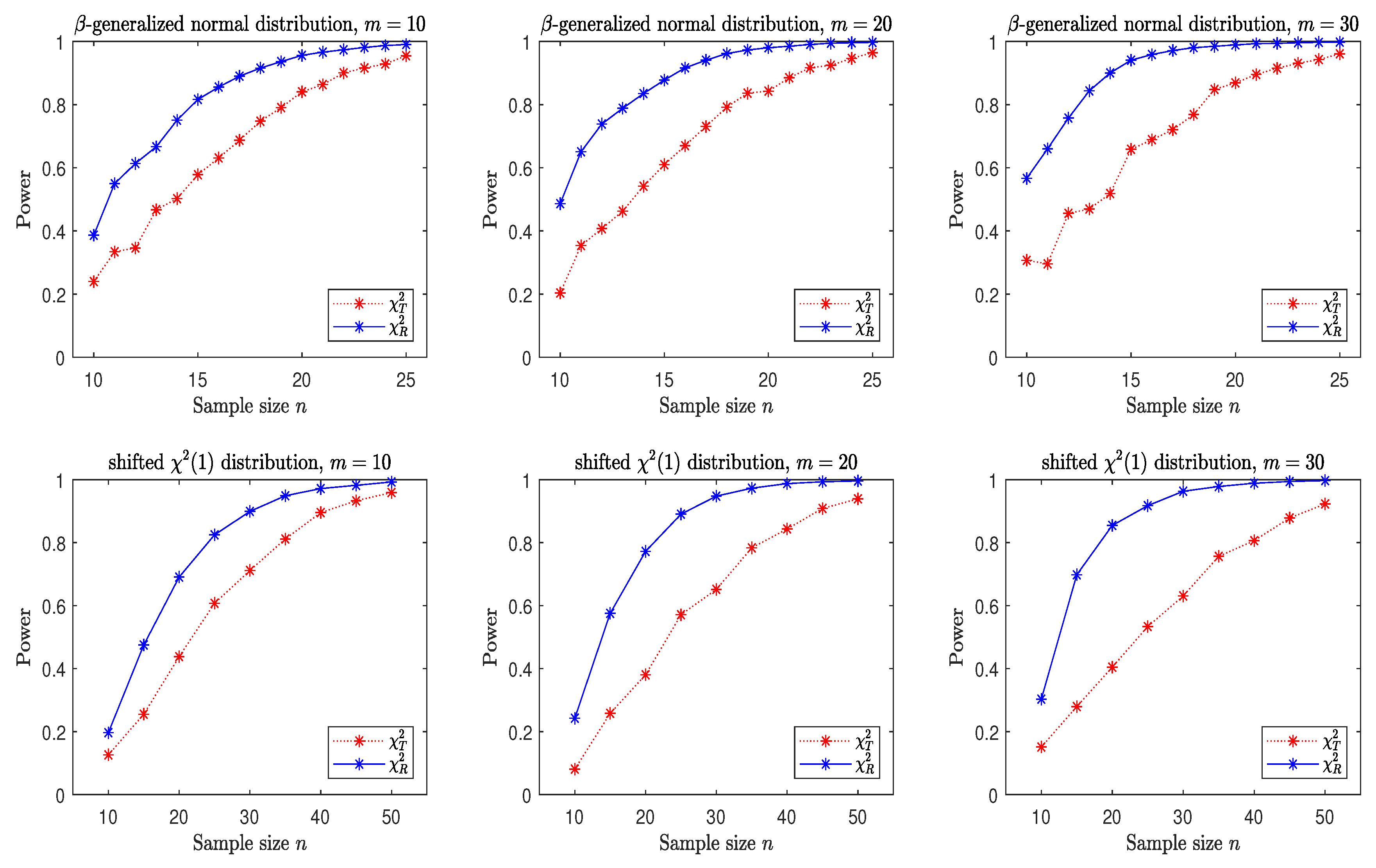
3.2. A Simple Power Comparison

In order for the power comparison to be representative, we select three symmetric distributions and three skewed distributions as follows, where the definitions for the multivariate t-distribution and the multivariate Cauchy distribution can be found in the work of Fang, Kotz, and Ng [17].

• The multivariate t-distribution has a density function of the form

  $$f_t(\parallel x\parallel )=C_1{\left(1+\frac{{\parallel x\parallel }^2}{m}\right)}^{-\frac{d+m}{2}},m>0,$$

  which is symmetric about the origin $f_t(\parallel x\parallel )\equiv f_t(\parallel -x\parallel )$, where “ $\parallel ·\parallel$ ” stands for the Euclidean norm of a vector. Let $m=5$.
• The multivariate Cauchy distribution has a density function of the form:

  $$f_c(\parallel x\parallel )=C_1{\left(1+\frac{{\parallel x\parallel }^2}{m}\right)}^{-\frac{d+1}{2}},$$

  which is symmetric about the origin, where $C_1$ is a normalizing constant depending on the dimension d.
• The $\beta$-generalized normal distribution $N_d\left(\mathbf{0},{\mathit{I}}_d,1/2\right)$ with $\beta =1/2$ has a density function of the form (by Goodman and Kotz [18]):

  $$f\left(x_1,\dots ,x_d\right)=\frac{{\beta }^d{r}^{d/\beta }}{2^d{\Gamma }^d(1/\beta )}·exp\left\{-r\sum _{i=1}^d{\left|x_i\right|}^{\beta }\right\},{\left(x_1,\dots ,x_d\right)}^{\prime }\in R^d,$$

  which is symmetric about the origin, where $r>0$ is a parameter. Let $r=1/2$ and $\beta =1$ in the simulation and denote it by $\beta$-g-normal.
• The shifted i.i.d. ${\chi }^2\left(1\right)$ has i.i.d. marginals, where each marginal has the same distribution as that of the random variable $Y=X-E\left(X\right)$, where $X\sim {\chi }^2\left(1\right)$, the univariate chi-square distribution with 1 degree of freedom and $E\left(X\right)=1$. This is a skewed distribution.
• The distribution $N(0,1)+{\chi }^2\left(2\right)$ consists of i.i.d. $[d/2]$ normal $N(0,1)$ marginals and $d-[d/2]$ i.i.d. ${\chi }^2\left(2\right)$ marginals. This is a skewed distribution.
• The shifted i.i.d. $exp\left(1\right)$ has i.i.d. marginals, where each marginal has the same distribution as that of the random variable $Y=X-E\left(X\right)$, where $X\sim exp\left(1\right)$, the univariate exponential distribution. This is a skewed distribution.

For each of these alternative distributions, we choose the sample size $n=50,70,\dots ,400$. We plot the power values versus the sample size n for both statistics ${\chi }_R^2$ and ${\chi }_T^2$ to obtain a quick visual comparison. Figure 1, Figure 2, Figure 3, Figure 4, Figure 5, Figure 6, Figure 7, Figure 8 and Figure 9 demonstrate the comparisons between the two power curves for ${\chi }_R^2$ (the blue one) and ${\chi }_T^2$ (the red one) with dimensions ranging from $d=5$ to $d=20$. The simulation is repeated 5000 times. It is observed that the RP chi-square test outperforms the traditional chi-square significantly for all selected symmetric alternative non-normal distributions (like the multivariate t, the Cauchy, and the $\beta$-generalized normal distribution) and asymmetric ones (like the chi-square and those with chi-square and exponential as the marginal distributions). Figure 10 and Figure 11 demonstrate the comparisons between the two projected chi-square tests ${\chi }_R^2$ (the blue one) and ${\chi }_T^2$ (the red one) under the multivariate t distribution with df = 5 (Figure 10) and the shifted ${\chi }^2\left(2\right)-2$ with i.i.d. marginals. Because both ${\chi }_R^2$ and ${\chi }_T^2$ for testing hypothesis (18) in Section 2 are affine invariant under the transformations (11)–(16) on the original x-sample in (11), we only need to take the zero mean and identity covariance matrix for the simulated samples. Figure 10 and Figure 11 show that the projected RP-${\chi }_R^2$ substantially outperforms the traditional ${\chi }_T^2$ for both recommended projection dimensions $q_1=[r/3]$ and $q_2=[r/2]$ with $r=min(n-1,d)-1$ under the significance level $\alpha =0.05$. The power improvement of the projected RP-${\chi }_R^2$ over the projected traditional ${\chi }_T^2$ is similar to the case demonstrated by Figure 10 and Figure 11 for other non-normal alternative distributions in Figure 1, Figure 2, Figure 3, Figure 4, Figure 5, Figure 6, Figure 7, Figure 8 and Figure 9. We do not present those similar cases to Figure 10 and Figure 11 to save some space.

It is pointed out that the Pearson chi-square statistic has an asymptotic chi-square distribution under any classification cell intervals. Its approximation speed to the chi-square distribution is $1/\sqrt{n}$ under a given sample size n ([16]). We choose the sample size n ranging from 50 to 400 in our Monte Carlo study to maintain fairly large sample sizes. While one may choose a larger sample size than 400 or a smaller sample size than 50 in the simulation, we just want to illustrate if our beta-RP-based MVN test is able to control the type I error rate feasibly within some range of the sample size. The choice of equiprobable classification cell intervals is motivated by the empirical study in [16] that shows some good performance of this choice. It is feasible to believe that our beta-RP-based MVN test will also show significant power improvement compared with the traditional chi-square test under a set of arbitrarily chosen cell intervals based on the study in [16].

3.3. An Illustrative Example

Example 1 

(see Example 6.3 of Fang and Wang [19] (pp. 258–262)). The data arose from the problem of standardizing the size for men’s clothes in China in 1976, which involves the data of 12 measurements of the body $\left(\mathrm{cm}\right)$:

$X_1:$ height from the waist up	$X_2:$ arm length
$X_3:$ bust	$X_4:$ neck
$X_5:$ shoulder length	$X_6:$ width of the front part of chest
$X_7:$ width of the back part of chest	$X_8:$ height
$X_9:$ height without head and neck	$X_{10}:$ height from the waist down
$X_{11}:$ waist circumference	$X_{12}:$ buttocks

A sample of size $n=100$ can be found in the work of Fang, Yuan, and Bentler [20]. Fang and Wang [19] implemented the classical skewness and kurtosis statistics and number-theoretic methods to test the multinormality of some subsets of the 12 variables. At $\alpha =0.05$ level of significance, they concluded that (1) $(X_1,X_3,X_8,X_{10},X_{12})$ has a multivariate normal distribution; (2) $(X_1,X_3,X_8,X_{10})$, $(X_1,X_8,X_{10},X_{12}$ and $(X_3,X_8,X_{10},X_{12})$ have a multivariate normal distribution; and (3) $(X_4,X_5,X_6,X_{11})$ and $(X_2,X_4,X_6,X_{11})$ have a non-normal distribution.

The p values under different m (the number of representation points) from the two chi-square tests, RP chi-square ${\chi }_R^2$ in Equation (10) and the traditional chi-square ${\chi }_T^2$ using equiprobable intervals defined by the endpoints given by Equation (19), are summarized in

Table 3. p values from the two chi-squared tests for the body data.

Subsets	${\mathit{\chi }}^2$	$\mathit{m}=10$	$\mathit{m}=20$	$\mathit{m}=30$
$\left(X_1,X_3,X_8,X_{10},X_{12}\right)$	${\chi }_R^2$	0.8498	0.8853	0.8027
	${\chi }_T^2$	0.8677	0.8487	0.5286
$\left(X_1,X_3,X_8,X_{10}\right)$	${\chi }_R^2$	0.9158	0.9016	0.8184
	${\chi }_T^2$	0.9558	0.7352	0.8518
$\left(X_1,X_8,X_{10},X_{12}\right)$	${\chi }_R^2$	0.8034	0.8133	0.7007
	${\chi }_T^2$	0.9241	0.5493	0.4342
$\left(X_3,X_8,X_{10},X_{12}\right)$	${\chi }_R^2$	0.5003	0.6428	0.8635
	${\chi }_T^2$	0.4012	0.5493	0.8518
$\left(X_4,X_5,X_6,X_{11}\right)$	${\chi }_R^2$	0.4355	0.1499	0.3865
	${\chi }_T^2$	0.4944	0.8678	0.6886
$\left(X_2,X_4,X_6,X_{11}\right)$	${\chi }_R^2$	0.6714	0.9141	0.7850
	${\chi }_T^2$	0.6371	0.7352	0.8733

. The results in Table 3 show that both the RP chi-square ${\chi }_R^2$ and the traditional chi-square ${\chi }_T^2$ give results consistent with those given by [19] on the multivariate normality of the four sets of variables: $(X_1,X_3,X_8,X_{10},X_{12})$, $(X_1,X_3,X_8,X_{10})$, $(X_1,X_8,X_{10},X_{12})$, and $(X_3,X_8,X_{10},X_{12})$, but both ${\chi }_R^2$ and ${\chi }_T^2$ fail to reject the possible non-normality of the two sets of variables $(X_4,X_5,X_6,X_{11})$ and $(X_2,X_4,X_6,X_{11})$, while Fang and Wang [19] reject the multivariate normality. This needs to be double checked by some other statistics for testing MVN.

4. Concluding Remarks

The theory of statistical representative points is a natural extension to the mean value of a probability distribution. A comprehensive study on the RP theory can be found in the work of Graf and Luschgy [21]. Application of the RP theory to testing multivariate normality was first proposed by Liang, He, and Yang [8] by using the univariate Student’s t-representative points, and by Wang et al. [9] using the univariate F-representative points. The study in this paper is parallel to those in [8] and of Wang et al. [9]. The results in these papers bridge the gap between the RP theory and testing goodness of fit. The Monte Carlo study in Section 3 shows some impressive power improvement from using the RP chi-square versus the traditional chi-square for both cases of relatively large and small sample sizes. A noticeable point is that the new RP-based test is still applicable in the case that the sample size may be smaller than the dimension, and it still performs very well. This can be regarded as a special credit compared with some existing tests for multivariate normality when faced with high dimension with a small sample size. Although it is not an easy task to prove whether the RP chi-square always improves the traditional chi-square in testing general goodness-of-fit problems, the results in this paper shed some hopeful light on applying the RP theory to the goodness-of-fit area. It is certain that the chi-square statistic is not the sole way to construct the RP-based test. Some other classical tests like those compared by Quesenberry and Miller [22] for general goodness-of-fit purposes can be also employed to test hypothesis (6). A complete comparison among these statistics for testing hypothesis (6) is beyond the scope of this paper. It is also too heavy to compare univariate tests and multivariate tests for high-dimensional normality. The beta RP-based test in this paper provides an additional way to connect the RP theory with goodness-of-fit techniques.

References

1. Ebner, B.; Henze, N. Tests for multivariate normality—A critical review with emphasis on weighted L2-statistics. Test 2020, 29, 845–892. [Google Scholar] [CrossRef]
2. Henze, N. Invariant tests for multivariate normality: A critical review. Stat. Pap. 2002, 43, 467–506. [Google Scholar] [CrossRef]
3. Horswell, R.L.; Looney, S.W. A comparison of tests for multivariate normality that are based on measures of multivariate skewness and kurtosis. J. Statist. Comput. Simul. 1992, 42, 21–38. [Google Scholar] [CrossRef]
4. Remeu, J.L.; Ozturk, A. A comparative study of goodness-of-fit tests for multivariate normality. J. Multivar. Anal. 1993, 46, 309–334. [Google Scholar] [CrossRef]
5. Mecklin, C.J.; Mundfrom, D.J. An appraisal and bibliography of tests for multivariate normality. Int. Stat. Rev. 2004, 72, 123–138. [Google Scholar] [CrossRef]
6. Fang, K.T.; He, S.D. The Problem of Selecting a Given Number of Representative Points in a Normal Population and a Generalized Mills Ratio; Stanford Technical Report; Stanford Statistics Department: Stanford, CA, USA, 1982; No. 327. [Google Scholar]
7. Flury, B.A. Principal points. Biometrika 1990, 77, 33–41. [Google Scholar] [CrossRef]
8. Liang, J.; He, P.; Yang, J. Testing multivariate normality based on t-representative points. Axioms 2022, 11, 587. [Google Scholar] [CrossRef]
9. Wang, S.; Liang, J.; Zhou, M.; Ye, H. Testing multivariate normality based on F-representative points. Mathematics 2022, 10, 4300. [Google Scholar] [CrossRef]
10. Mardia, K.V. Measures of multivariate skewness and kurtosis with applications. Biometrika 1970, 57, 519–530. [Google Scholar] [CrossRef]
11. Mardia, K.V. Tests of univariate and multivariate normality. In Handbook of Statistics; Krishnaiah, P.R., Ed.; North-Holland Publishing Company: Amsterdam, The Netherlands, 1980; pp. 279–320. [Google Scholar]
12. Small, N.J.H. Plotting squared radii. Biometrika 1978, 65, 657–658. [Google Scholar] [CrossRef]
13. Ahn, S.K. F-probability plot and its application to multivariate normality. Commun. Stat. Theory Methods 1992, 21, 997–1023. [Google Scholar] [CrossRef]
14. Wilks, S.S. Mathematical Statistics; Wiley: New York, NY, USA, 1962. [Google Scholar]
15. Liang, J.; Li, R.; Fang, H.; Fang, K.T. Testing multinormality based on low-dimensional projection. J. Stat. Plan. Inference 2000, 86, 129–141. [Google Scholar] [CrossRef]
16. Voinov, V.; Pya, N.; Alloyarova, R. A comparative study of some modified chi-squared tests. Commun. Stat. Simul. Comput. 2009, 38, 355–367. [Google Scholar] [CrossRef]
17. Fang, K.T.; Kotz, S.; Ng, K.W. Symmetric Multivariate and Related Distributions; Chapman and Hall: London, UK; New York, NY, USA, 1990. [Google Scholar]
18. Goodman, I.R.; Kotz, S. Multivariate q-generalized normal distribution. J. Multivar. Stat. Anal. 1990, 3, 204–219. [Google Scholar] [CrossRef]
19. Fang, K.T.; Wang, Y. Number-Theoretic Methods in Statistics; Chapman and Hall: London, UK, 1994. [Google Scholar]
20. Fang, K.T.; Yuan, K.; Bentler, P.M. Applications of sets of points uniformly distributed on a sphere to testing multinormality and robust estimation. In Probability and Statistics; Jiang, Z.P., Yan, S.J., Cheng, P., Wu, R., Eds.; World Scientific: Singapore, 1992; pp. 56–73. [Google Scholar]
21. Graf, S.; Luschgy, H. Foundations of Quantization for Probability Distributions; Springer: Berlin/Heidelberg, Germany, 2007. [Google Scholar]
22. Quesenberry, C.P.; Miller, F.L., Jr. Power studies of some tests for uniformity. J. Stat. Comput. Simul. 1977, 5, 169–191. [Google Scholar] [CrossRef]
Figure 1. Dimension d = 5 .
Mathematics 12 01711 g001
Figure 2. Dimension d = 5 .
Mathematics 12 01711 g002
Figure 3. Dimension d = 5 .
Mathematics 12 01711 g003
Figure 4. Dimension d = 10 .
Mathematics 12 01711 g004
Figure 5. Dimension d = 10 .
Mathematics 12 01711 g005
Figure 6. Dimension d = 10 .
Mathematics 12 01711 g006
Figure 7. Dimension d = 20 .
Mathematics 12 01711 g007
Figure 8. Dimension d = 20 .
Mathematics 12 01711 g008
Figure 9. Dimension d = 20 .
Mathematics 12 01711 g009
Figure 10. Power comparison between two projected χ 2 tests for multivariate normality ( d = 30 , r = min ( n 1 , d ) 1 ).
Mathematics 12 01711 g010
Figure 11. Power comparison between two projected χ 2 tests for multivariate normality ( d = 50 , r = min ( n 1 , d ) 1 ).
Mathematics 12 01711 g011