Stochastic Patterns of Bitcoin Volatility: Evidence across Measures

Abstract

This research conducted a thorough investigation of Bitcoin volatility patterns using three interrelated methodologies: R/S investigation, simple moving average (SMA), and the relative strength index (RSI). The paper jointly employes the above techniques on volatility range-based estimators to effectively capture the unpredictable volatility patterns of Bitcoin. R/S analysis, SMA, and RSI calculations assess time series data obtained from our volatility estimators. Although Bitcoin is known for its high volatility and price instability, our analysis using R/S analysis and moving averages suggests the existence of underlying patterns. The estimated Hurst exponents for our volatility estimators indicate a level of persistence in these patterns, with some estimators displaying more persistence than others. This persistence underscores the potential of momentum-based trading strategies, reinforcing the expectation of additional price rises after declines and vice versa. However, significant volatility often interrupts this upward movement. The SMA analysis also demonstrates Bitcoin’s susceptibility to external market forces. These observations indicate that traders and investors should modify their risk management approaches in accordance with market circumstances, perhaps integrating a combination of momentum-based and mean-reversion tactics to reduce the risks linked to Bitcoin’s volatility. Furthermore, the existence of robust patterns, as demonstrated by our investigation, presents promising opportunities for investing in Bitcoin.

1. Introduction

Bitcoin has notably influenced the conventional financial sector, with its price fluctuations attracting significant attention from asset managers and portfolio risk managers. This digital currency has experienced various abrupt high levels of volatility, prompting a need for a thorough econometric analysis to understand and predict its price behavior and underlying influencing factors such as regulatory changes, technological advancements, and macroeconomic variables. Exploring the Bitcoin’s price through econometric models allows for a structured analysis of patterns and potential causality in its volatility dynamics, contributing to more informed decision-making processes among investors and policymakers. Bitcoin’s influence is expanding, reaching various economic sectors, so understanding its volatility dynamics is critical for predicting potential impacts for investors [1]. As a result, a detailed examination of its volatility is a necessary endeavor to chart the course of cryptocurrencies in the broader financial system [2]. However, conducting an analysis of Bitcoin volatility is not without challenges. Volatility is an integral part of the research conducted because the purpose of this paper is to understand Bitcoin price dynamics. Firstly, the concept of volatility must be defined. Volatility is defined as a unit of measurement of market risk and has the potential to cause great concern to all individuals who have some form of market participation or not [3]. However, according to Floros et al. (2020) [4], volatility is a variable that is difficult to observe, making it almost impossible to predict its impact on financial markets [5]. Also, volatility plays a key role in the financial sector and everyone’s interest is focused on the level and nature of volatility [6,7]. Finally, over the years, volatility may change leading to modeling with stochastic models [8,9]. Moreover, the market’s immaturity, characterized by a lack of established theoretical frameworks and stringent regulations, adds complexity to modeling efforts. Additionally, Bitcoin’s well-known volatility presents a challenge in creating models that can accurately capture its price dynamics without being unduly influenced by large values. Acknowledging these challenges is fundamental to ensure that the resulting insights are not only robust but also relevant in the practical context. Given the fact of this irregular behavior of Bitcoin, it is necessary to examine and codify better potential trends in Bitcoin data. Trend analysis is a powerful tool for investors to take advantage from patterns of price dynamics structure or manage accordingly their portfolios.

There is a gap in the literature for applying trend analysis on Bitcoin using various volatility estimators. To address the above research gap, we capture the volatile nature of Bitcoin prices through range-based volatility estimators. We then employ three basic methods for detecting trends in the behavior of the volatility estimators, R/S-analysis (the Hurst exponent), Simple Moving Average (SMA), and the Relative Strength Index (RSI). The Hurst exponent is a widely used statistical measure which quantifies the long-term memory of the time series and helps investors to manage their portfolio [10]. This type of exponent quantifies its result through the following three financial strategies: momentum-based strategy, random walk, and mean-reversion strategy. The momentum-based strategy detects price trend dynamics, and then investors try to take advantage of the continuous trends in the market. Random walk indicates an uncorrelated (random) time series, and the mean-reversion strategy reflects that asset price volatility will return to the long-term level after a large event. In addition, investors might diversify their portfolios based on the Hurst exponent values, considering a mix of momentum-based and mean-reverse strategies and keeping away from risky investments determined by random walk. Risk aversion is also the main objective of the additional methodologies examined in this paper.

As we mentioned before, Bitcoin has experienced extreme levels of volatility and may be sensitive to the exogenous conditions. Therefore, by applying R/S Analysis, Moving Averages, and RSI on Bitcoin’s volatility, we examine how these mechanisms react to this sensitivity produced by exogenous factors. In addition, we investigate how these mechanisms illustrate the irregular behavior of Bitcoin’s volatility. For this reason, the purpose of this work is to provide to investors a better understanding of volatility dynamics, creating in this way more effective trading strategies and portfolio risk management. Thus, this paper contributes to the research area of financial mathematics using advanced quantitative techniques, by (i) employing various volatility estimators instead of prices solely using intraday data, for capturing the volatility dynamics in cryptocurrency markets—intraday data allow to us to offer a better understanding of market behavior within shorter time frames, (ii) combining multiple volatility estimators allowing for a holistic understanding of cryptocurrency market behaviors and dynamics, (iii) incorporating multiple analytical methodologies which may in turn enhance our understating of cryptocurrency price volatilities, by capturing multiple facets of cryptocurrency price behavior and assessing their potential risks and trend persistence over a time horizon such as clustering effects and volatility persistence.

Note that the connection of R/S analysis and range-based estimators has been studied by [10]. But in our case, the contribution in the sense of financial mathematics is due to the expansion of the volatility measures (i.e., the method of range-based estimators) on SMA and RSI methods. In this way, we extracted a specific type of time-series applied on SMA and RSI methods. The results from these three methods, in combination with the volatility measures, captures potential diverse financial situations which helps investors to manage and diverse their strategy and their portfolio.

This is also a contribution to the general literature of pattern analysis. In addition, we apply the method of volatility measures to Bitcoin price data, which are extremely sensitive to exogenous conditions. This is one more novelty of this work, related to the financial part. More precisely, this paper contributes to the research area of financial mathematics by (i) employing volatility estimators instead of prices solely, for capturing the volatility of cryptocurrency price volatilities, (ii) combining multiple volatility estimators allowing for a holistic understanding of cryptocurrency market behaviors and dynamics, (iii) incorporating multiple analytical methodologies which may in turn enhance our understating of cryptocurrency price volatilities, by capturing multiple facets of cryptocurrency price behavior and assessing their potential risks and trend persistence over a time horizon.

2. Literature Review

The recent literature in financial markets, particularly focusing on cryptocurrencies, demonstrates a growing interest in understanding market dynamics through advanced econometric analysis and mathematical modeling. These studies collectively contribute to a more nuanced comprehension of market behavior, risk management, and trading strategies in the volatile and complex world of cryptocurrencies. Schelling’s (2019) exploration of the linear-quadratic ergodic control problem using fractional Brownian motion, especially in the context of rough volatility models, highlights the significant impact of transaction costs on portfolio strategies [11]. This is particularly relevant in cryptocurrency markets, where rough volatility is a common characteristic, and transaction costs can significantly influence investment decisions.

The empirical study by Zhou and Liu on foreign exchange prices, utilizing Brownian motion theory, provides valuable insights into currency price behaviors [7,12]. Their approach, which involves comparing simulated and actual prices, underscores the potential of Brownian motion theory in predicting price movements in cryptocurrencies, a market known for its unpredictability and rapid price changes.

Bianchi’s (2012) work on the Efficient Market Hypothesis and its challenges, especially in the realm of behavioral finance, offers a comprehensive framework for understanding market efficiency amidst investor behavior [13]. This perspective is crucial in the cryptocurrency market, where investor sentiment and behavior play a pivotal role in price fluctuations.

The workshop by Graham, Thiery, and Beskos on statistical modeling for stochastic processes, with a focus on fractional Brownian motion in high-frequency trading and asset pricing, is particularly pertinent to cryptocurrencies [14]. High-frequency trading is a dominant aspect of cryptocurrency markets, and understanding its implications is key to developing effective trading strategies.

Wang’s (2018) investigation into the asymptotic behavior of hedging errors in models related to geometric fractional Brownian motion sheds light on the risks and strategies associated with hedging in cryptocurrency markets [15]. This study is vital for investors and traders who are navigating the complex risk landscape of cryptocurrencies.

The research by Çağlar, Bahtiyar, and Altintas (2014) on parameter estimation in agent-based stock price models, involving long-range dependence and self-similarity, is applicable to the cryptocurrency market [16]. Their findings help in understanding the collective behavior of market participants, a critical factor in the highly interconnected and community-driven cryptocurrency ecosystem.

Qin’s research on a two-date consumption model with continuous trading, where information is revealed through an Ornstein–Uhlenbeck bridge, illuminates the impact of heterogeneous beliefs on asset pricing. In the cryptocurrency market, where diverse investor beliefs and information asymmetry are prevalent, this study provides valuable insights into price dynamics.

J. Qiu’s (2018) application of R/S analysis in analyzing SME board stock price movements and developing a trading strategy based on the Hurst index introduces the fractal market hypothesis as a novel approach to cryptocurrency market analysis [7,17,18]. This perspective offers a fresh lens through which to view and interpret the complex patterns and trends in cryptocurrency prices.

Lastly, Sun and Dong’s (2023) use of fractional Brownian motion to model energy-switching costs in the context of carbon allowance trading demonstrates the adaptability of stochastic optimization models [19]. This approach can be applied to similar trading mechanisms in cryptocurrency markets, particularly in the context of environmental sustainability and carbon footprint considerations. In addition, and given the fact that the Bitcoin price has irregular behavior, forecasting its volatility is pivotal for traders, investors, and the general financial community. The work of [20] is looking for the most suitable model of the Bitcoin volatility forecast among several GARCH and two heterogeneous autoregressive models. Finally, EGARCH and APARCH were more effective than the others. GARCH and EGARCH models have been used by the study of [21] in order to examine Bitcoin volatility behavior while examining if social network sentiment and the S&P500 index (and also the VIX index) have an impact on Bitcoin volatility. They found that in speculative periods, Bitcoin volatility is irregular and that in stable periods S&P500 and VIX returns and sentiment have an impact on Bitcoin volatility. In [22], the authors study the effect of the introduction of Bitcoin futures on Bitcoin return and volatility based on realized volatility and GARCH model pre- and post-futures. The work of [23] shows that the volatility of Bitcoin prices is extreme and almost ten times higher than the volatility of major exchange rates. In [24], the authors mainly focus on the role of jumps in forecasting Bitcoin volatility using linear and nonlinear mixed data sampling models.

Let us now point out some of the limitations of our methodology. The employed methodological approach however suffers inefficiencies associated to the limitations of each one of the employed tools. The limitations of the R/S analysis method involve the method’s (i) sensitivity to data with non-stationary behaviors [25], (ii) inefficiency to provide reliable estimations of the Hurst exponent, for small size datasets [26], (iii) assumption of a fractal data structure [27], and (iv) sensitivity to changes in the dataset’s sequence [28]. Regarding the SMA model employed, its critical limitations are associated to the model’s (i) lag behind current market conditions, which may in turn lead to delayed signals for market entry or exit [29], (ii) inability to quickly adapt to rapid price changes [30], (iii) assignment of equal weights to all past data, thus not fully facilitating the significance of the information of the most previous data, and justifying why SMA may be less effective in the case of choppy markets [31]. Finally, for the RSI method, its limitations are associated to the model’s (i) potential premature signaling of overbought or undersold conditions when the markets are characterized by strong trends [32], (ii) potential to produce false signals in non-trending or range bound markets [33], (iii) requirement of additional technical indicators and models for avoiding misleading interpretations of the model’s results [34].

Future research perspectives should focus on addressing the identified limitations of the models employed in our proposed methodological approach. Specifically with respect to the R/S analysis, and for addressing its non-stationarity limitation, an adaptive fractal analysis can be jointly employed for dynamically adjusting the model’s parameters [35]. Regarding the small dataset limitation of R/S analysis, machine learning algorithms such as random forests, decision trees, and support vector machines could be used in combination with bootstrapping and synthetic data generation techniques [36]. Finally, regarding the third limitation of the R/S analysis associated to its sensitivity to dataset sequence changes, wavelet decomposition can be employed to assess time series at different scales [37]. For SMA, future research perspectives should focus on the development of adaptive weighted SMA variations that adjust the weights to emphasize to more recent historical data [38], or even the combination of SMAs with simple exponential moving averages to improve signal responsiveness [29]. Finally, for the RSI analysis, future research perspectives could involve (i) the modification of the RSI function to conduct conditional checks before providing overbought or oversold signals [39] and (ii) the additional consideration of macroeconomic indicators along with sentiments from news and social media for improving the accuracy of predictions [31].

The critical analysis of the examined literature reveals the following research gaps:

• While individual studies have focused on specific technical indicators like R/S Analysis, SMA, and RSI, there is a gap in research that integrates these tools comprehensively to analyze cryptocurrency prices and trends in combination with various volatility estimators;
• Research on the long-term memory of cryptocurrency markets using tools like the Hurst exponent and its implications for market efficiency is still nascent. More studies are needed to understand how these aspects affect trading strategies in the cryptocurrency context;
• There seems to be a lack of research tools that combine various statistical and econometric tools to develop comprehensive risk management strategies tailored to the unique characteristics of Bitcoin’s volatility dynamics.

This paper addresses the above research gaps as follows:

• Integration of Multiple Technical Indicators: By employing a combination of R/S Analysis, SMA, and RSI, our paper provides a comprehensive approach to analyzing cryptocurrency dynamics and trends in function of volatility estimators. This integrated methodology offers a more holistic view of market dynamics than studies focusing on individual indicators;
• Long-Term Memory and Market Efficiency in Cryptocurrencies: By utilizing tools like the Hurst exponent, our paper delves into the long-term memory of Bitcoin markets and its implications for market efficiency. This helps in developing trading strategies that are better suited to the cryptocurrency market’s behavior;
• Comprehensive Risk Management Strategies: The combination of various statistical and econometric tools in this paper aids in the development of comprehensive risk management strategies for cryptocurrency trading, addressing the high volatility and unpredictability of these markets.

3. Methodology of Bitcoin Volatility Behavior Analysis

In this section we present the mathematical background of different methodologies for detecting patterns in Bitcoin volatility time series. The first mathematical tool, i.e., R/S analysis, employed for assessing the existence of trends in Bitcoin’s behavior. R/S analysis, or rescaled range analysis, is a statistical method used to detect and analyze the persistence, or long-term memory, of time series data. The primary purpose of this analysis is to determine the degree of correlation within a time series and to identify whether the series exhibits a random walk, mean-reverting, or trending behavior. The mathematical analysis of R/S will be based on the works of Szostakowski (2019) and Roel F. Ceballos and Fe F. Largo as analyzed below [40,41].

Let the time series X of length N divided into sub-period of length d, where n is an integral divisor of N. Then we calculate the mean value such that:

$$\mathrm{m}=\frac{1}{\mathrm{n}}\sum _{\mathrm{i}=1}^{\mathrm{n}}{\mathrm{X}}_{\mathrm{i}},$$

(1)

Then we normalize the data as the following Equation (2):

$${\mathrm{Y}}_{\mathrm{t}}={\mathrm{X}}_{\mathrm{t}}-\mathrm{m},$$

(2)

for t = 1, ⋯ n, returning in this way the cumulative time series Z where:

$${\mathrm{Z}}_{\mathrm{t}}=\sum _{\mathrm{i}=1}^{\mathrm{t}}{\mathrm{Y}}_{\mathrm{i}},\mathrm{t}=1,\cdots \mathrm{n},$$

(3)

Then, the respective range will be: ${\mathrm{R}}_{\mathrm{n}}=\mathrm{m}\mathrm{a}\mathrm{x}({\mathrm{Z}}_1,\cdots ,{\mathrm{Z}}_{\mathrm{n}})-\mathrm{m}\mathrm{i}\mathrm{n}({\mathrm{Z}}_1,\cdots ,{\mathrm{Z}}_{\mathrm{n}})$ and after that we rescale the range by using the standard deviation S_n:

$${\left(\frac{\mathrm{R}}{\mathrm{S}}\right)}_{\mathrm{n}}=\frac{{\mathrm{R}}_{\mathrm{n}}}{{\mathrm{S}}_{\mathrm{n}}},$$

(4)

Finally, we can estimate the Hurst exponent through R/S analysis:

$$\mathrm{E}{\left(\frac{\mathrm{R}}{\mathrm{S}}\right)}_{\mathrm{n}}=\mathrm{c}{\mathrm{n}}^{\mathrm{H}}, \mathrm{for} \mathrm{the} \mathrm{constant} \mathrm{c} \mathrm{independent} \mathrm{of} \mathrm{n}.$$

(5)

Let us now distinguish the different results of the different cases of H. For example, if $\mathrm{H}=1/2,$ then the series is uncorrelated, that is the series is characterized by random behavior. If $\mathrm{H}<1/2 (0<\mathrm{H}<0.5),$ then we have the case of anti-persistence in the time series, that is, it has the tendency to return to the long-term mean. On the other hand, if $\mathrm{H}>1/2$ (0.5 < H < 1) then the time series has a positive long-term autocorrelation (persistent series) [42].

The second step of our analysis involves the employment of simple moving average (SMA) analysis on volatility estimators to identify potential trading signals and discern underlying price trends. By calculating short-term (1-h) and long-term (24-h) SMAs, we can smooth short-term volatility and reveal significant trend movements over time [43]. The 1-h SMA closely follows the actual price jump data, providing insight into the immediate market reactions, while the 24-h SMA offers a broader view, highlighting the more sustained and significant trend patterns. Crossover points between these two SMAs are particularly telling; an upward crossing of the short-term SMA over the long-term SMA signals a potential entry point or ‘buy’ signal, suggesting an emerging bullish trend. Conversely, a downward crossing indicates a potential exit point or ‘sell’ signal, implying a bearish trend development [44]. These signals are instrumental for traders and analysts who rely on technical analysis to make informed decisions about market entry and exit points. The application of SMA analysis to volatility estimators thus serves as a valuable tool for understanding market dynamics and developing strategic trading actions based on historical price behavior [45]. Mathematically, SMA is calculated by using the t-th time step of the most recent n values (a past window of size n) as described by the following equation:

$${\mathrm{S}\mathrm{M}\mathrm{A}}_{\mathrm{t},\mathrm{n}}=\frac{1}{\mathrm{n}}\left\{{\mathrm{X}}_{\mathrm{t}}+{\mathrm{X}}_{\mathrm{t}-1}+\cdots +{\mathrm{X}}_{\mathrm{t}-\left(\mathrm{n}-1\right)}\right\}=\frac{1}{\mathrm{n}}\sum _{\mathrm{i}=1}^{\mathrm{n}}{\mathrm{X}}_{\mathrm{t}-\left(\mathrm{i}-1\right),}$$

(6)

where n belongs to the integer set (n ∈ Z), and X_i represents the data of the i-th time step [46,47,48].

The final third step of our methodological approach involves the development of the Relative Strength Index. Through the employment of this index, investors identify whether an asset, in this case Bitcoin, is in an overbought or oversold condition. When the RSI value is high (typically above 70), it suggests that Bitcoin may be overbought, indicating a potential reversal or correction in price. Conversely, when the RSI is low (typically below 30), it suggests that Bitcoin may be oversold, indicating a potential rebound in price. Moreover, it helps traders and analysts assess the strength and speed of price movements [49]. When Bitcoin experiences a rapid price jump, the RSI can help gauge the momentum behind that jump. A sharp increase in the RSI can indicate strong buying pressure and bullish momentum, while a sharp decrease can indicate strong selling pressure and bearish momentum. If the RSI shows a divergence from the actual price movement, it can be a signal that a trend reversal might be imminent [50]. For example, if Bitcoin’s price exhibits higher highs, but the RSI is reveals lower highs, it is called bearish divergence, which may suggest a potential price drop [51]. Finally, RSI can help traders manage risk. For instance, if Bitcoin has experienced a series of price jumps, and the RSI is consistently in overbought territory, it may caution traders against entering long new positions, as it suggests that a correction might be overdue [52]. The formula for RSI is presented below [53]:

$$\mathrm{R}\mathrm{S}\mathrm{I}=100-\frac{100}{1+\frac{{\mathrm{A}\mathrm{v}\mathrm{e}\mathrm{r}\mathrm{a}\mathrm{g}\mathrm{e}}_{\mathrm{g}\mathrm{a}\mathrm{i}\mathrm{n}}}{{\mathrm{A}\mathrm{v}\mathrm{e}\mathrm{r}\mathrm{a}\mathrm{g}\mathrm{e}}_{\mathrm{l}\mathrm{o}\mathrm{s}\mathrm{s}}}}.$$

Here we can define that RS = relative strength = $\frac{{\mathrm{A}\mathrm{v}\mathrm{e}\mathrm{r}\mathrm{a}\mathrm{g}\mathrm{e}}_{\mathrm{g}\mathrm{a}\mathrm{i}\mathrm{n}}}{{\mathrm{A}\mathrm{v}\mathrm{e}\mathrm{r}\mathrm{a}\mathrm{g}\mathrm{e}}_{\mathrm{l}\mathrm{o}\mathrm{s}\mathrm{s}}}$.

We now describe the methodology used to extract volatility measures used in this study. First of all, we mention some important assumptions. The value $\mathrm{P}$ follows a simple continuous stochastic process called Brownian motion and as a result, the log-price $\mathrm{p}=\mathrm{l}\mathrm{n}\left(\mathrm{P}\right)$ follows a similar process Brownian motion with zero drift and diffusion $\mathsf{\sigma }$.

$${\mathrm{d}\mathrm{p}}_{\mathrm{t}}={\mathsf{\sigma }\mathrm{d}\mathrm{B}}_{\mathrm{t}}$$

(7)

The subsequent assumption pertains to the non-volatility of the diffusion parameter σ throughout the day, even though σ varies from one day to another. We designate a day as the unit of time. Through observation, we find that in the above equation, the diffusion parameter resembles the standard deviation of returns, indicating normalization, thus rendering it unnecessary to differentiate between quantities. The basic variables are subsequently defined in the following equations as: “Open” stands for the daily opening price, “Close” denotes the daily closing price, “High” represents the highest daily price, and “Low” indicates the lowest daily price. These variables are crucial for computing returns, namely Open-to-Close, Open-to-High, and Open-to-Low. (Refer to

Table 1. Descriptive Statistics of Bitcoin Prices.

	Open	High	Low	Close
count	3421.0	3421.0	3421.0	3421.0
mean	14,804.1	15,149.2	14,432.4	14,814.9
std	16,322.8	16,712.6	15,885.8	16,324.6
min	176.9	211.7	171.5	178.1
25%	922.2	940.0	915.8	922.0
50%	8315.7	8509.1	8140.9	8309.3
75%	24,640.0	25,190.3	24,225.1	24,664.8
max	67,549.7	68,789.6	66,382.1	67,566.8

for descriptive statistics.)

$${\mathrm{p}}_{\mathrm{c}\mathrm{l}\mathrm{o}\mathrm{s}\mathrm{e}}=\ln \left(\mathrm{C}\mathrm{l}\mathrm{o}\mathrm{s}\mathrm{e}\right)-\ln \left(\mathrm{O}\mathrm{p}\mathrm{e}\mathrm{n}\right)$$

(8)

$${\mathrm{p}}_{\mathrm{m}\mathrm{a}\mathrm{x}}=\ln \left(\mathrm{H}\mathrm{i}\mathrm{g}\mathrm{h}\right)-\ln \left(\mathrm{O}\mathrm{p}\mathrm{e}\mathrm{n}\right)$$

(9)

$${\mathrm{p}}_{\mathrm{m}\mathrm{i}\mathrm{n}}=\ln \left(\mathrm{L}\mathrm{o}\mathrm{w}\right)-\ln \left(\mathrm{O}\mathrm{p}\mathrm{e}\mathrm{n}\right)$$

(10)

where ${\mathrm{p}}_{\mathrm{c}\mathrm{l}\mathrm{o}\mathrm{s}\mathrm{e}}$ represents the return which is a random normally distributed variable with mean $0$ and variance (volatility) ${\mathsf{\sigma }}^2$.

$$\mathrm{c}~\mathrm{N}(0,{\mathsf{\sigma }}^2)$$

(11)

We aim to evaluate the volatility ${\mathsf{\sigma }}^2$, which is not directly observable, using three observable variables: variables ${\mathrm{p}}_{\mathrm{c}\mathrm{l}\mathrm{o}\mathrm{s}\mathrm{e}},{\mathrm{p}}_{\mathrm{m}\mathrm{a}\mathrm{x}},\mathrm{a}\mathrm{n}\mathrm{d} {\mathrm{p}}_{\mathrm{m}\mathrm{i}\mathrm{n}}$. It is important to highlight that ${\mathrm{p}}_{\mathrm{c}\mathrm{l}\mathrm{o}\mathrm{s}\mathrm{e}}^2$ serves as an unbiased estimator of ${\mathsf{\sigma }}^2$:

$$\mathrm{E}\left({\mathrm{p}}_{\mathrm{c}\mathrm{l}\mathrm{o}\mathrm{s}\mathrm{e}}^2\right)={\mathsf{\sigma }}^2$$

(12)

In the following equation, the initial volatility estimator, denoted by “s” for “simple”, is outlined below:

$$\widehat{{\mathsf{\sigma }}_{\mathrm{s}}^2}={\mathrm{p}}_{\mathrm{c}\mathrm{l}\mathrm{o}\mathrm{s}\mathrm{e}}^2$$

(13)

Given the inherent noise in the simple estimator, we seek a more reliable alternative. The volatility derived from the difference between upper and lower price points relative to the closing price offers substantial information. Additionally, valuable insights can be gleaned from the high and low prices. It is widely recognized that the range distribution, represented by $\mathrm{d}\equiv {\mathrm{p}}_{\mathrm{m}\mathrm{a}\mathrm{x}}-{\mathrm{p}}_{\mathrm{m}\mathrm{i}\mathrm{n}}$ of the Brownian motion, determines the difference between higher and lower prices [54]. During the day, we define $\mathrm{P}\left(\mathrm{y}\right)$ as the probability that the difference $\mathrm{d}\le \mathrm{y}$ is practicable:

$$\mathrm{P}\left(\mathrm{y}\right)=\sum _{\mathrm{n}=1}^{\mathrm{\infty }}{(-1)}^{\mathrm{n}+1}\mathrm{n}\left\{\mathrm{E}\mathrm{r}\mathrm{f}{\mathrm{p}}_{\mathrm{c}\mathrm{l}\mathrm{o}\mathrm{s}\mathrm{e}}(\frac{\left(\mathrm{n}+1\right)\mathrm{y}}{\sqrt{2\mathsf{\sigma }}})-2\mathrm{E}\mathrm{r}\mathrm{f}{\mathrm{p}}_{\mathrm{c}\mathrm{l}\mathrm{o}\mathrm{s}\mathrm{e}}\left(\frac{\mathrm{n}\mathrm{y}}{\sqrt{2\mathsf{\sigma }}}\right)+\mathrm{E}\mathrm{r}\mathrm{f}{\mathrm{p}}_{\mathrm{c}\mathrm{l}\mathrm{o}\mathrm{s}\mathrm{e}}(\frac{\left(\mathrm{n}-1\right)\mathrm{y}}{\sqrt{2\mathsf{\sigma }}})\right\}$$

(14)

where:

$$\mathrm{E}\mathrm{r}\mathrm{f}{\mathrm{p}}_{\mathrm{c}\mathrm{l}\mathrm{o}\mathrm{s}\mathrm{e}}=1-\mathrm{E}\mathrm{r}\mathrm{f}\left(\mathrm{y}\right)$$

(15)

where $\mathrm{E}\mathrm{r}\mathrm{f}\left(\mathrm{y}\right)$ represents the error function. We utilize the Parkinson (1980) distribution for the calculation (for $\mathrm{p}\ge 1$):

$$\mathrm{E}\left({\mathrm{d}}^{\mathrm{P}}\right)=\frac{4}{\sqrt{\mathrm{\pi }}}\mathrm{\Gamma }\left(\frac{\mathrm{p}+1}{2}\right)\left(1-\frac{4}{2^{\mathrm{p}}}\right)\mathsf{\zeta }(\mathrm{p}-1)(2{\mathsf{\sigma }}^2)$$

(16)

where $\mathrm{\Gamma }\left(\mathrm{y}\right)$ and $\mathrm{\zeta }\left(\mathrm{y}\right)$ represent the gamma function and the Riemann zeta function, respectively.

For $\mathrm{p}=1$:

$$\mathrm{E}\left(\mathrm{d}\right)=\sqrt{8\mathrm{\pi }}\mathsf{\sigma }$$

(17)

and for $\mathrm{p}=2$:

$$\mathrm{E}\left({\mathrm{d}}^2\right)=4\ln \left(2\right){\mathsf{\sigma }}^2$$

(18)

Based on Equation (18), Garman and Klass (1980) suggested a new volatility estimator [55]:

$$\widehat{{\mathsf{\sigma }}_{\mathrm{p}}^2}=\frac{{({\mathrm{p}}_{\mathrm{m}\mathrm{a}\mathrm{x}}-{\mathrm{p}}_{\mathrm{m}\mathrm{i}\mathrm{n}})}^2}{4\mathrm{l}\mathrm{n}2}$$

(19)

The base estimator relies solely on the difference between ${\mathrm{p}}_{\mathrm{m}\mathrm{a}\mathrm{x}}-{\mathrm{p}}_{\mathrm{m}\mathrm{i}\mathrm{n}}$, suggesting that a more precise estimator could be achieved by incorporating all available information [55]. However, seeking a minimum variance estimator based on ${\mathrm{p}}_{\mathrm{c}\mathrm{l}\mathrm{o}\mathrm{s}\mathrm{e}}$, ${\mathrm{p}}_{\mathrm{m}\mathrm{a}\mathrm{x}}$, and ${\mathrm{p}}_{\mathrm{m}\mathrm{i}\mathrm{n}}$, poses a persistent challenge, as it presents an infinite-dimensional problem. This challenge is addressed by imposing constraints on estimators that are functions of ${\mathrm{p}}_{\mathrm{c}\mathrm{l}\mathrm{o}\mathrm{s}\mathrm{e}}$, ${\mathrm{p}}_{\mathrm{m}\mathrm{a}\mathrm{x}}$, and ${\mathrm{p}}_{\mathrm{m}\mathrm{i}\mathrm{n}}$ known as analytical estimators. The subsequent equation defines the minimum analytical variance estimator, which is:

$$\widehat{{\mathsf{\sigma }}_{\mathrm{G}\mathrm{K}\mathrm{p}\mathrm{r}\mathrm{e}\mathrm{c}\mathrm{i}\mathrm{s}\mathrm{e}}^2}=0.511{({\mathrm{p}}_{\mathrm{m}\mathrm{a}\mathrm{x}}-{\mathrm{p}}_{\mathrm{m}\mathrm{i}\mathrm{n}})}^2-0.019\left({\mathrm{p}}_{\mathrm{c}\mathrm{l}\mathrm{o}\mathrm{s}\mathrm{e}}\left({\mathrm{p}}_{\mathrm{m}\mathrm{a}\mathrm{x}}+{\mathrm{p}}_{\mathrm{m}\mathrm{i}\mathrm{n}}\right)-2{\mathrm{p}}_{\mathrm{m}\mathrm{a}\mathrm{x}}{\mathrm{p}}_{\mathrm{m}\mathrm{i}\mathrm{n}}\right)-0.383{\mathrm{p}}_{\mathrm{c}\mathrm{l}\mathrm{o}\mathrm{s}\mathrm{e}}^2$$

(20)

We note that the right term (cross-products) is deemed insignificant, prompting us to introduce a more suitable estimator in the following equation:

$$\widehat{{\mathsf{\sigma }}_{\mathrm{G}\mathrm{K}}^2}=0.5{({\mathrm{p}}_{\mathrm{m}\mathrm{a}\mathrm{x}}-{\mathrm{p}}_{\mathrm{m}\mathrm{i}\mathrm{n}})}^2-(2\mathrm{l}\mathrm{n}2-1){\mathrm{p}}_{\mathrm{c}\mathrm{l}\mathrm{o}\mathrm{s}\mathrm{e}}^2$$

(21)

Equation (13) presents the volatility estimator known as Garman-Klass, denoted as GK [55]. The GK estimator offers a notable advantage over other estimators, as it represents the optimal combination with the lowest variance between two fundamental estimators: a simple estimator and the Parkinson volatility estimator [4].

Meilijson (2009) introduces a novel estimator characterized by the smallest variance [56]. This estimator is defined in Equation (22) as follows:

$$\widehat{{\mathsf{\sigma }}_{\mathrm{M}}^2}=0.274{\mathsf{\sigma }}_1^2+0.16{\mathsf{\sigma }}_{\mathrm{s}}^2+0.365{\mathsf{\sigma }}_3^2+0.2{\mathsf{\sigma }}_4^2$$

(22)

where:

$${\mathsf{\sigma }}_1^2=2[{\left({\mathrm{p}}_{\mathrm{m}\mathrm{a}\mathrm{x}}^{\prime }-{\mathrm{p}}_{\mathrm{c}\mathrm{l}\mathrm{o}\mathrm{s}\mathrm{e}}^{\prime }\right)}^2+{\mathrm{p}}_{\mathrm{l}\mathrm{o}\mathrm{w}}^{\prime }]$$

(23)

$${\mathsf{\sigma }}_3^2=2({\mathrm{p}}_{\mathrm{m}\mathrm{a}\mathrm{x}}^{\prime }-{\mathrm{p}}_{\mathrm{c}\mathrm{l}\mathrm{o}\mathrm{s}\mathrm{e}}^{\prime }-{\mathrm{p}}_{\mathrm{m}\mathrm{i}\mathrm{n}}^{\prime }){\mathrm{p}}_{\mathrm{c}\mathrm{l}\mathrm{o}\mathrm{s}\mathrm{e}}^{\prime }$$

(24)

$${\mathsf{\sigma }}_4^2=-\frac{({\mathrm{p}}_{\mathrm{m}\mathrm{a}\mathrm{x}}^{\prime }-{\mathrm{p}}_{\mathrm{c}\mathrm{l}\mathrm{o}\mathrm{s}\mathrm{e}}^{\prime }){\mathrm{p}}_{\mathrm{m}\mathrm{i}\mathrm{n}}^{\prime }}{2\mathrm{l}\mathrm{n}2-\raisebox{1ex}{$5$}\!\left/ \!\raisebox{-1ex}{$4$}\right.}$$

(25)

where ${\mathrm{p}}_{\mathrm{c}\mathrm{l}\mathrm{o}\mathrm{s}\mathrm{e}}^{\prime }={\mathrm{p}}_{\mathrm{c}\mathrm{l}\mathrm{o}\mathrm{s}\mathrm{e}},{\mathrm{p}}_{\mathrm{m}\mathrm{a}\mathrm{x}}^{\prime }={\mathrm{p}}_{\mathrm{m}\mathrm{a}\mathrm{x}},{\mathrm{p}}_{\mathrm{m}\mathrm{i}\mathrm{n}}^{\prime }={\mathrm{p}}_{\mathrm{m}\mathrm{i}\mathrm{n}} \mathrm{if} {\mathrm{p}}_{\mathrm{c}\mathrm{l}\mathrm{o}\mathrm{s}\mathrm{e}}>0 \mathrm{and} {\mathrm{p}}_{\mathrm{c}\mathrm{l}\mathrm{o}\mathrm{s}\mathrm{e}}^{\prime }=-{\mathrm{p}}_{\mathrm{c}\mathrm{l}\mathrm{o}\mathrm{s}\mathrm{e}},{\mathrm{p}}_{\mathrm{m}\mathrm{a}\mathrm{x}}^{\prime }=-{\mathrm{p}}_{\mathrm{m}\mathrm{i}\mathrm{n}},{\mathrm{p}}_{\mathrm{m}\mathrm{i}\mathrm{n}}^{\prime }=-{\mathrm{p}}_{\mathrm{m}\mathrm{a}\mathrm{x}} \mathrm{if} {\mathrm{p}}_{\mathrm{c}\mathrm{l}\mathrm{o}\mathrm{s}\mathrm{e}}<0$.

The following Equation (26) presents the RS estimator and with this estimator arbitrary drift is allowed:

$$\widehat{{\mathsf{\sigma }}_{\mathrm{R}\mathrm{S}}^2}={\mathrm{p}}_{\mathrm{m}\mathrm{a}\mathrm{x}}\left({\mathrm{p}}_{\mathrm{m}\mathrm{a}\mathrm{x}}-{\mathrm{p}}_{\mathrm{c}\mathrm{l}\mathrm{o}\mathrm{s}\mathrm{e}}\right)+{\mathrm{p}}_{\mathrm{m}\mathrm{i}\mathrm{n}}({\mathrm{p}}_{\mathrm{m}\mathrm{i}\mathrm{n}}-{\mathrm{p}}_{\mathrm{c}\mathrm{l}\mathrm{o}\mathrm{s}\mathrm{e}})$$

(26)

4. Numerical Implementation

The applicability of the developed methodologies is evaluated in the case of 3421 daily open, high, low, and close bitcoin data from September 2014 to January 2024.

The descriptive statistics table for Bitcoin prices over 3421 observations reveal insights into the cryptocurrency’s trading behavior. The average opening price (Open) is USD 14,804.1, with a high degree of volatility as indicated by a standard deviation of USD 16,322.8. The opening prices ranged from a minimum of USD 176.9 to a maximum of USD 67,549.7, with the median at USD 8315.7. This wide range suggests significant fluctuations in Bitcoin’s opening prices over the observed period. Similarly, the highest price (High) during the trading period averages at USD 15,149.2, with a standard deviation of USD 16,712.6, highlighting the volatile nature of Bitcoin’s value. The high prices span from as low as USD 211.7 to as high as USD 68,789.6. The lowest trading prices (Low) also show considerable variability, with an average of USD 14,432.4 and a range from USD 171.5 to USD 66,382.1. The closing prices (Close) closely mirror the opening prices in terms of average (USD 14,814.9) and volatility (standard deviation of USD 16,324.6), ranging from USD 178.1 to USD 67,566.8. The quartile values across all categories further illustrate the wide dispersion and the skewed distribution of Bitcoin prices, with a significant jump in values from the 25th percentile to the 75th percentile, indicating that a substantial portion of the price points are clustered at the lower end of the spectrum but with a long tail extending to much higher values.

The first step of our numerical analysis involved the implementation of R/S analysis, or rescaled range analysis, in order is to identify whether the series exhibits a random walk, mean-reverting, or trending behavior.

Table 2. Hurst exponent values for each Bitcoin volatility estimator.

	$\widehat{{\mathsf{\sigma }}_{\mathbf{p}}^{\mathbf{2}}}$	$\widehat{{\mathsf{\sigma }}_{\mathbf{G}\mathbf{K}}^{\mathbf{2}}}$	$\widehat{{\mathsf{\sigma }}_{\mathbf{M}}^{\mathbf{2}}}$	$\widehat{{\mathsf{\sigma }}_{\mathbf{R}\mathbf{S}}^{\mathbf{2}}}$
Hurst Exponent	0.636	0.590	0.586	0.632

provides the derived hurst exponent values, for each one of the derived volatility estimators

The Hurst exponents calculated for the four volatility estimators indicate persistence in the time series data. This suggests that all series tend to continue their current trends over time. Estimators 1 and 4 exhibit a stronger persistence, implying a higher likelihood of maintaining their trends. In contrast, estimators 2 and 3 also show persistence but to a lesser extent. Such characteristics are particularly relevant in financial markets, where these trends might inform momentum-based trading strategies, highlighting the potential for increases to be followed by further increases and decreases by further decreases [57].

Regarding the second step of our methodological approach, Figure 1, Figure 2, Figure 3 and Figure 4 depict daily predicted vs actual two-period SMAs for the examined four $\widehat{{\mathsf{\sigma }}_{\mathrm{p}}^2}$, $\widehat{{\mathsf{\sigma }}_{\mathrm{G}\mathrm{K}}^2}$, $\widehat{{\mathsf{\sigma }}_{\mathrm{M}}^2}$, and $\widehat{{\mathsf{\sigma }}_{\mathrm{R}\mathrm{S}}^2}$ Bitcoin volatility estimators (VEs) used in this study. The two periods were optimally determined using the minimum mean absolute percentage error (MAPE) criterion.

The SMA not only reveals underlying market trends but also potentially signals critical moments for investors to enter or exit the market. For VE_1 and VE_4, whose SMA curves suggest a more gradual and consistent market movement, a rising SMA could be interpreted as a sign of increasing market stability or an impending upward trend, offering a potential entry signal for long-term investors. Conversely, a declining SMA might indicate decreasing volatility, potentially serving as an exit signal for those looking to capitalize on peak market movements before a period of consolidation.VE_2 and VE_3, characterized by their sharper volatility spikes, present a different scenario. An upward trend in their SMAs might signal increasing market uncertainty or the start of a volatile period, possibly serving as an exit signal for risk-averse investors or an entry signal for those seeking to capitalize on market turmoil. Alternatively, a downward trend in the SMA could indicate a subsiding of volatility, potentially signaling a safer entry point for investors waiting for market stabilization or a cue for exiting to those who have capitalized on the preceding volatility.

The nuanced predictive value of the SMA across these estimators suggests that while they may not offer precise predictions, the direction and trend of the SMA can serve as a strategic guide. Investors might use increases in the SMA as indicators to hedge against anticipated volatility or to prepare for a strategic entry into the market, depending on their risk tolerance and investment horizon. Conversely, decreases in the SMA could inform decisions to lock in gains before a potential decrease in market activity or to enter the market during periods of expected stability.

The results derived from the implementation of the final third methodological approach, namely the RSI, on our data are summarized in the following Figure 5.

The key insights derived are summarized as follows:

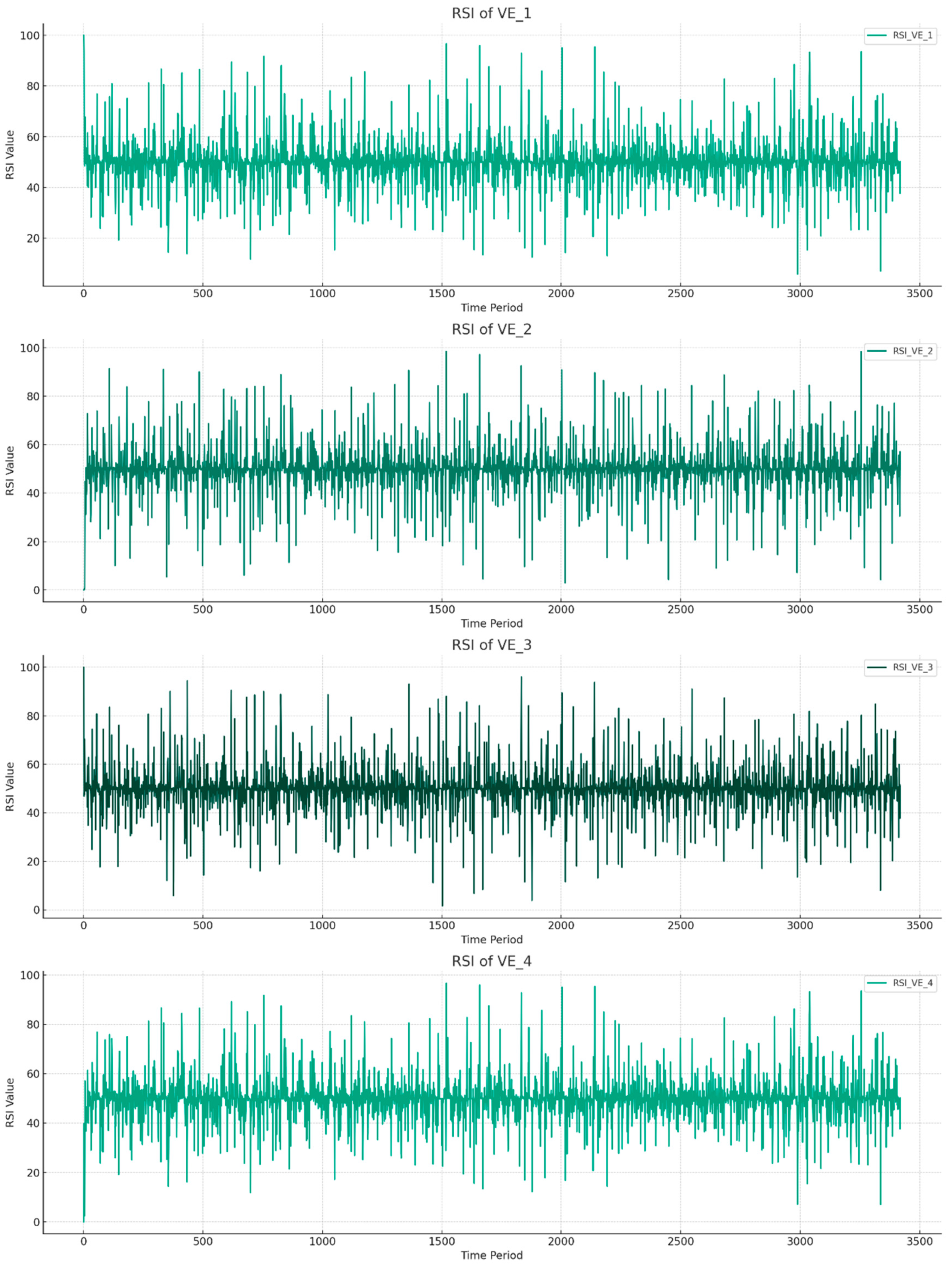
• Overbought Conditions: Volatility Estimator VE_1 exhibits the highest average overbought events, followed by VE_2, VE_3, and VE_4. This suggests that VE_1 tends to reach overbought conditions more frequently, indicating periods where the asset may be considered overvalued according to this estimator;
• Oversold Conditions: VE_4 shows a tendency for the highest average annual oversold events, suggesting it more frequently reaches conditions considered to be undervalued. This might indicate a propensity for VE_4 to experience significant valuation drops or higher volatility, leading to potential buying opportunities as per this metric;
• Momentum Fluctuations: VE_1 and VE_3 demonstrate a higher frequency of sharp increases, indicating more frequent sudden valuation changes according to these estimators. For sharp decreases, the distribution across the volatility estimators is more varied, with VE_2 and VE_4 showing slightly higher tendencies for these events. This indicates that VE_2 and VE_4 may experience more pronounced volatility in terms of sharp valuation decreases;
• Risk Management Insights: VE_1, exhibiting frequent overbought events and sharp increases, suggests this estimator might be more prone to rapid valuation changes. Consequently, risk management strategies that take into account VE_1’s characteristics might need to prepare for more frequent transitions between overvalued conditions and potentially rapidly changing market sentiments.

5. Discussion

In this study, we embarked on a comprehensive analysis of Bitcoin volatility trends, employing three interconnected methodologies: R/S analysis, Simple Moving Average (SMA), and the Relative Strength Index (RSI). The descriptive statistics reveal significant fluctuations in Bitcoin prices within the period studied, underscoring the cryptocurrency’s well-documented volatility. This volatility is characterized by large swings, as evidenced by the spread between the 25th and 75th percentiles. Despite Bitcoin’s inherent price instability and the large volatility values observed, our findings from the R/S analysis and moving averages indicate the presence of underlying trends. The Hurst exponents calculated for our volatility estimators suggest a persistence in these trends, with some estimators showing stronger persistence than others [9]. This persistence indicates a potential for momentum-based trading strategies, affirming the idea that price increases are likely to be followed by subsequent increases, and vice versa for decreases. Periods of high volatility occasionally disrupt this momentum, obscuring the underlying trend dynamics, particularly in the intervals between 2000–3000- and 3000–3500-time units. The SMA analysis further reveals Bitcoin’s sensitivity to external market conditions. For instance, the market sentiment at the close of trading, as depicted in our figures, encapsulates the culmination of daily trading activities, news, and events. This end-of-day sentiment contrasts with the sentiment at the opening, peak optimism during the session, and the lowest confidence points, each represented by different price points. These insights suggest that traders and investors need to adapt their risk management strategies in response to market conditions, potentially incorporating a mix of momentum-based and mean-reversion strategies to mitigate the risks associated with Bitcoin’s volatility. Moreover, the presence of strong trends, as evidenced by our analysis, offers optimistic prospects for investing in Bitcoin. These trends not only highlight the cryptocurrency’s dynamic behavior but also suggest the feasibility of employing specific financial strategies for profit maximization or risk avoidance. Our RSI analysis, in particular, points to frequent overbought conditions, indicating times when Bitcoin might be considered overvalued, and underscoring the importance of sharp price movements in informing investment decisions. In summary, our discussion underscores the complex interplay between Bitcoin’s volatility, market trends, and the influence of external factors on its price dynamics. By leveraging R/S analysis, SMA, and RSI, investors can gain deeper insights into Bitcoin’s market behavior, enabling more informed trading and investment strategies amidst the cryptocurrency’s unpredictable fluctuations. Future research perspectives could involve the inclusion of additional variables that could have an impact on Bitcoin prices such as macroeconomic indicators and volumes. Moreover, extending our analysis to additional cryptocurrencies could provide broader generalized insights for the digital crypto market.

References

1. Andersen, T.G.; Bollerslev, T. Heterogeneous Information Arrivals and Return Volatility Dynamics: Uncovering the Long-Run in High Frequency Returns. J. Financ. 1997, 52, 975–1005. [Google Scholar] [CrossRef]
2. Doumenis, Y.; Izadi, J.; Dhamdhere, P.; Katsikas, E.; Koufopoulos, D. A Critical Analysis of Volatility Surprise in Bitcoin Cryptocurrency and Other Financial Assets. Risks 2021, 9, 207. [Google Scholar] [CrossRef]
3. Giot, P.; Laurent, S.; Petitjean, M. Trading activity, realized volatility and jumps. J. Empir. Financ. 2010, 17, 168–175. [Google Scholar] [CrossRef]
4. Floros, C. Modelling volatility using high, low, open and closing prices: Evidence from four S&P indices. Int. Res. J. Financ. Econ. 2009, 28, 198–206. Available online: https://researchportal.port.ac.uk/en/publications/modelling-volatility-using-high-low-open-and-closing-prices-evide (accessed on 6 February 2024).
5. Gkillas, K.; Floros, C.; Suleman, M.T. Quantile dependencies between discontinuities and time-varying rare disaster risks. Eur. J. Financ. 2021, 27, 932–962. [Google Scholar] [CrossRef]
6. Alghalith, M. Pricing the American options: A closed-form, simple formula. Phys. A Stat. Mech. Appl. 2020, 548, 123873. [Google Scholar] [CrossRef]
7. Sariannidis, N.; Giannarakis, G.; Zafeiriou, E.; Billias, I. The Effect of Crude Oil Price Moments on Socially Responsible Firms in Eurozone. Int. J. Energy Econ. Policy 2016, 6, 356–363. Available online: https://dergipark.org.tr/en/pub/ijeeep/issue/31917/351090 (accessed on 6 February 2024).
8. Tsagkanos, A.; Gkillas, K.; Konstantatos, C.; Floros, C. Does Trading Volume Drive Systemic Banks’ Stock Return Volatility? Lessons from the Greek Banking System. Int. J. Financ. Stud. 2021, 9, 24. [Google Scholar] [CrossRef]
9. Kanavos, P.; Fontrier, A.M.; Gill, J.; Efthymiadou, O. Does external reference pricing deliver what it promises? Evidence on its impact at national level. Eur. J. Health Econ. HEPAC Health Econ. Prev. Care 2020, 21, 129–151. [Google Scholar] [CrossRef] [PubMed]
10. Zournatzidou, G.; Floros, C. Hurst Exponent Analysis: Evidence from Volatility Indices and the Volatility of Volatility Indices. J. Risk Financ. Manag. 2023, 16, 272. [Google Scholar] [CrossRef]
11. Schelling, D.M. Rough Volatility and Portfolio Optimisation under Small Transaction Costs. Ph.D. Thesis, The London School of Economics and Potilical Science, London, UK, 2019. [Google Scholar]
12. Zhou, J.; Liu, W. Study on the Daily Exchange Rate Movement Based on the Model of Brownian Motion. In Proceedings of the 2015 3rd International Conference on Education, Management, Arts, Economics and Social Science, Changsha, China, 28–29 December 2015; pp. 931–936. [Google Scholar] [CrossRef]
13. Bianchi, N. Electrical machine analysis using finite elements. In Electrical Machine Analysis Using Finite Elements; CRC Press: Boca Raton, FL, USA, 2017; pp. 1–275. [Google Scholar] [CrossRef]
14. Beskos, A.; Roberts, G.; Thiery, A.H.; Pillai, N. Asymptotic analysis of the random walk Metropolis algorithm on ridged densities. Ann. Appl. Probab. 2018, 28, 2966–3001. [Google Scholar] [CrossRef]
15. Wang, W. Asymptotic analysis for hedging errors in models with respect to geometric fractional Brownian motion. Stochastics 2019, 91, 407–432. [Google Scholar] [CrossRef]
16. Çaǧlar, M.; Bahtiyar, N.; Altintaş, I. Parameter estimation of an agent-based stock price model. Appl. Stoch. Models Bus. Ind. 2014, 30, 227–239. [Google Scholar] [CrossRef]
17. Qiu, J.-Y. The SME Board Stock Price Trend Analysis and Investment Strategy Under the Fractal Market Hypothesis. DEStech Trans. Soc. Sci. 2017. [Google Scholar] [CrossRef]
18. Kiohos, A.; Sariannidis, N. Determinants of the asymmetric gold market. Invest. Manag. Financ. Innov. 2010, 7, 26–33. Available online: https://scholar.google.gr/citations?view_op=view_citation&hl=el&user=xU_kC08AAAAJ&citation_for_view=xU_kC08AAAAJ:M3ejUd6NZC8C (accessed on 6 February 2024).
19. Sun, S.L.; Ding, Z.; Joseph, G. Expanding Inclusive Markets through Corruption Control: A Multilevel Modeling Analysis for a Grand Challenge. J. Int. Manag. 2023, 29, 101068. [Google Scholar] [CrossRef]
20. Bergsli, L.Ø.; Lind, A.F.; Molnár, P.; Polasik, M. Forecasting volatility of Bitcoin. Res. Int. Bus. Financ. 2022, 59, 101540. [Google Scholar] [CrossRef]
21. López-Cabarcos, M.Á.; Pérez-Pico, A.M.; Piñeiro-Chousa, J.; Šević, A. Bitcoin volatility, stock market and investor sentiment. Are they connected? Financ. Res. Lett. 2021, 38, 101399. [Google Scholar] [CrossRef]
22. Bouteska, A.; Harasheh, M. Bitcoin volatility and the introduction of bitcoin futures: A portfolio construction approach. Financ. Res. Lett. 2023, 57, 104200. [Google Scholar] [CrossRef]
23. Baur, D.G.; Dimpfl, T. The volatility of Bitcoin and its role as a medium of exchange and a store of value. Empir. Econ. 2021, 61, 2663–2683. [Google Scholar] [CrossRef]
24. Qian, L.; Wang, J.; Ma, F.; Li, Z. Bitcoin volatility predictability–The role of jumps and regimes. Financ. Res. Lett. 2022, 47, 102687. [Google Scholar] [CrossRef]
25. Raubitzek, S.; Corpaci, L.; Hofer, R.; Mallinger, K. Scaling Exponents of Time Series Data: A Machine Learning Approach. Entropy 2023, 25, 1671. [Google Scholar] [CrossRef] [PubMed]
26. Gómez-Águila, A.; Trinidad-Segovia, J.E.; Sánchez-Granero, M.A. Improvement in Hurst exponent estimation and its application to financial markets. Financ. Innov. 2022, 8, 1–21. [Google Scholar] [CrossRef]
27. Kobeissi, H.Y. Multifractal Financial Markets; Springer: New York, NY, USA, 2013. [Google Scholar] [CrossRef]
28. Peters, E.E. Chaos and Order in the Capital Markets: A New View of Cycles, Prices, and Market Volatility, 2nd ed.; Wiley: Hoboken, NJ, USA, 1996; Available online: https://www.amazon.com/Chaos-Order-Capital-Markets-Volatility/dp/0471139386 (accessed on 6 February 2024).
29. Murphy, J.J. Technical analysis of the financial markets. Pa. Dent. J. 1999, 77, 33–34. Available online: http://www.ncbi.nlm.nih.gov/pubmed/20599625 (accessed on 6 February 2024).
30. Pring, M.J. Technical Analysis Explained: The Successful Investor’s Guide to Spotting Investment Trends and Turning Points, 5th ed.; McGraw Hill: New York, NY, USA, 2014. [Google Scholar]
31. Aronson, D.R. Evidence-Based Technical Analysis: Applying the Scientific Method and Statistical Inference to Trading Signals; Wiley: Hoboken, NJ, USA, 2011. [Google Scholar] [CrossRef]
32. Achelis, S.B. Technical Analysis from A to Z, 2nd ed.; McGraw Hill: New York, NY, USA, 2013. [Google Scholar]
33. Kirkpatrick, C.D.; Dahlquist, J.R. Technical Analysis, The Complete Resource for Market Technicians; FT Press: Upper Saddle River, NJ, USA, 2007; p. 49. Available online: https://books.google.co.th/books/about/Technical_Analysis.html?id=I5SgX5q5sQEC&redir_esc=y (accessed on 6 February 2024).
34. Bollinger, J. Bollinger on Bollinger Bands; McGraw Hill: New York, NY, USA, 2002; Volume 227. [Google Scholar]
35. Turiel, A.; Pérez-Vicente, C.J. Role of multifractal sources in the analysis of stock market time series. Phys. A Stat. Mech. Appl. 2005, 355, 475–496. [Google Scholar] [CrossRef]
36. Barunik, J.; Kristoufek, L. On Hurst exponent estimation under heavy-tailed distributions. Phys. A Stat. Mech. Appl. 2012, 389, 3844–3855. [Google Scholar] [CrossRef]
37. Gençay, R.; Selçuk, F.; Whitcher, B. Differentiating intraday seasonalities through wavelet multi-scaling. Phys. A Stat. Mech. Appl. 2001, 289, 543–556. [Google Scholar] [CrossRef]
38. Kaufman, P.J. Trading Systems and Methods. 2013. Available online: https://www.wiley.com/en-us/Trading+Systems+and+Methods%2C+5th+Edition-p-9781118043561 (accessed on 6 February 2024).
39. Carter, J.F. Mastering the Trade: Proven Techniques for Profiting from Intraday and Swing Trading Setups; McGraw Hill: New York, NY, USA, 2012; Volume 459. [Google Scholar]
40. Szóstakowski, R. The use of the Hurst exponent to investigate the quality of forecasting methods of ultra-high-frequency data of exchange rates. Przegląd Stat. 2019, 65, 200–223. [Google Scholar] [CrossRef]
41. Ceballos, R.F.; Largo, F.F. On The Estimation of the Hurst Exponent Using Adjusted Rescaled Range Analysis, Detrended Fluctuation Analysis and Variance Time Plot: A Case of Exponential Distribution. arXiv 2018, arXiv:1805.08931. Available online: https://arxiv.org/abs/1805.08931v1 (accessed on 6 February 2024).
42. Zournatzidou, G.; Mallidis, I.; Farazakis, D.; Floros, C. Enhancing Bitcoin Price Volatility Estimator Predictions: A Four-Step Methodological Approach Utilizing Elastic Net Regression. Mathematics 2024, 12, 1392. [Google Scholar] [CrossRef]
43. Resta, M.; Pagnottoni, P.; De Giuli, M.E. Technical Analysis on the Bitcoin Market: Trading Opportunities or Investors’ Pitfall? Risks 2020, 8, 44. [Google Scholar] [CrossRef]
44. Kardile, R.; Ugale, T.; Mohanty, S.N. Stock Price Predictions using Crossover SMA. In Proceedings of the 2021 9th International Conference on Reliability 2021, Infocom Technologies and Optimization (Trends and Future Directions), ICRITO, Noida, India, 3–4 September 2021. [Google Scholar] [CrossRef]
45. Okereke, A.-E.; Cornelius, O.C.; Ephraim, A.C. Comparative study on Optimized Moving Average types, Buy-and- Hold Trading Strategies. Int. J. Sci. Eng. Res. 2019, 10. Available online: http://www.ijser.org (accessed on 6 February 2024).
46. Agustian, H.; Pujiastuti, A.; Varian Sayoga, M.; Studi Informatika, P.; Tinggi Teknologi Adisutjipto, S. Comparison of Simple Moving Average and Exponential Smoothing Methods To Predict Seaweed Prices. CCIT (Creat. Commun. Innov. Technol.) J. 2020, 13, 175–184. [Google Scholar] [CrossRef]
47. Nau, R. Forecasting with Moving Averages; Fuqua School of Business, Duke University: Durham, NC, USA, 2014; pp. 1–3. [Google Scholar]
48. Su, Y.; Cui, C.; Qu, H. Self-Attentive Moving Average for Time Series Prediction. Appl. Sci. 2022, 12, 3602. [Google Scholar] [CrossRef]
49. Tilehnouei, M.H.; Shivaraj, B. A Comparative Study of Two Technical Analysis Tools: Moving Average Convergence and Divergence V/S Relative Strength Index: A Case Study of Hdfc Bank Ltd Listed In National Stock Exchange Of India (Nse). Int. J. Manag. Bus. Res. 2013, 3, 191–197. [Google Scholar]
50. Uma, K.S.; Naidu, S. Prediction of intraday trend reversal in stock market index through machine learning algorithms. Adv. Intell. Syst. Comput. 2021, 1200, 331–341. [Google Scholar] [CrossRef]
51. Jain, R.; Bhardwaj, P.; Soni, P. Can the Market of Cryptocurrency Be Followed with the Technical Analysis? Int. J. Res. Appl. Sci. Eng. Technol. 2022, 10, 2425–2445. [Google Scholar] [CrossRef]
52. Kazeminia, S.; Sajedi, H.; Arjmand, M. Real-Time Bitcoin Price Prediction Using Hybrid 2D-CNN LSTM Model. In Proceedings of the 2023 9th International Conference on Web Research (ICWR), Tehran, Iran, 3–4 May 2023; pp. 173–178. [Google Scholar] [CrossRef]
53. Bolton, J.; von Boetticher, S.T. Momentum Trading on the Johannesburg Stock Exchange after the Global Financial Crisis. Procedia Econ. Financ. 2015, 24, 83–92. [Google Scholar] [CrossRef]
54. Feller, W. The Asymptotic Distribution of the Range of Sums of Independent Random Variables. Ann. Math. Stat. 1951, 22, 427–432. [Google Scholar] [CrossRef]
55. Garman, M.B.; Klass, M.J. On the Estimation of Security Price Volatilities from Historical Data. J. Bus. 1980, 53, 67–78. Available online: https://www.jstor.org/stable/2352358 (accessed on 6 February 2024). [CrossRef]
56. Meilijson, I. The Garman-Klass volatility estimator revisited. Revstat Stat. J. 2008, 9, 199–212. Available online: https://arxiv.org/abs/0807.3492v2 (accessed on 6 February 2024).
57. Malik, F.; Ewing, B.T.; Payne, J.E. Measuring volatility persistence in the presence of sudden changes in the variance of Canadian stock returns. Can. J. Econ. Rev. Can. D’économique 2005, 38, 1037–1056. [Google Scholar] [CrossRef]
Figure 1. Daily actual vs. predicted σ p 2 volatility data.
Mathematics 12 01719 g001
Figure 2. Daily actual vs. predicted σ G K 2 volatility data.
Mathematics 12 01719 g002
Figure 3. Daily actual vs. predicted σ M 2 volatility data.
Mathematics 12 01719 g003
Figure 4. Daily actual vs. predicted σ R S 2 volatility data.
Mathematics 12 01719 g004
Figure 5. RSI analysis of volatility estimators.
Mathematics 12 01719 g005