Some Simpson- and Ostrowski-Type Integral Inequalities for Generalized Convex Functions in Multiplicative Calculus with Their Computational Analysis

Abstract

Integral inequalities are very useful in finding the error bounds for numerical integration formulas. In this paper, we prove some multiplicative integral inequalities for first-time differentiable s-convex functions. These new inequalities help in finding the error bounds for different numerical integration formulas in multiplicative calculus. The use of s-convex function extends the results for convex functions and covers a large class of functions, which is the main motivation for using s-convexity. To prove the inequalities, we derive two different integral identities for multiplicative differentiable functions in the setting of multiplicative calculus. Then, with the help of these integral identities, we prove some integral inequalities of the Simpson and Ostrowski types for multiplicative generalized convex functions. Moreover, we provide some numerical examples and computational analysis of these newly established inequalities, to show the validity of the results for multiplicative s-convex functions. We also give some applications to quadrature formula and special means of real numbers within the framework of multiplicative calculus.

1. Introduction

Inequalities play a crucial role in establishing the bounds and properties of functions in the field of mathematical analysis. One notable class of inequalities is the Ostrowski-type inequality, which has proven to be a valuable tool in various branches of mathematics. Ostrowski introduced this useful and attractive integral inequality in 1938 (see [1], p. 468). Suppose $Ϝ:J\subseteq \mathbb{R}\to \mathbb{R}$ is a differentiable function on $J^o$ and on the interior of the given interval J, such that $Ϝ\in L[{\theta }_1,{\theta }_2]$; here, ${\theta }_1,{\theta }_2\in J$ with ${\theta }_2>{\theta }_1$. If $|{Ϝ}^{\prime }\left(\kappa \right)|\le M$ for all $\kappa \in [{\theta }_1,{\theta }_2]$ then the following inequality holds:

$$\left|Ϝ\left(\varkappa \right)-\frac{1}{{\theta }_2-{\theta }_1}{\int }_{{\theta }_1}^{{\theta }_2}Ϝ\left(\kappa \right)d\kappa \right|\le M\left({\theta }_2-{\theta }_1\right)\left(\frac{1}{4}+\frac{{\left(\varkappa -\frac{{\theta }_1+{\theta }_2}{2}\right)}^2}{{\left({\theta }_2-{\theta }_1\right)}^2}\right),$$

(1)

for all $\varkappa \in \left[{\theta }_1,{\theta }_2\right]$. The constant $\frac{1}{4}$ is the best possible. This inequality produces an upper bound that can be used for approximation of the given integral average $\frac{1}{{\theta }_2-{\theta }_1}{\int }_{{\theta }_1}^{{\theta }_2}Ϝ\left(\kappa \right)d\kappa$ by the value of $Ϝ\left(\kappa \right)$ at a point $\kappa \in [{\theta }_1,{\theta }_2]$. Many researchers have studied such inequalities in recent years, and several generalizations, extensions and variations have emerged in a number of papers, such as [2,3].

Convexity is a fundamental concept in mathematics, particularly in the fields of calculus, optimization and mathematical analysis. Mathematically, a function $Ϝ\left(\kappa \right)$ defined on an interval $[{\theta }_1,{\theta }_2]$ is convex if for any pair of points $({\theta }_1,Ϝ\left({\theta }_1\right))$ and $({\theta }_2,Ϝ\left({\theta }_2\right))$ lying within the interval the function satisfies the inequality

$$Ϝ(\kappa {\theta }_1+(1-\kappa ){\theta }_2)\le \kappa Ϝ\left({\theta }_1\right)+(1-\kappa )Ϝ\left({\theta }_2\right),$$

(2)

for each value of $\kappa$ between 0 and 1. In recent decades, many scholars have explored the inequalities associated with convexity in many directions (see [4,5,6,7,8] and the references listed therein). The Hermite–Hadamard inequality, which is frequently used in many areas of applied mathematics, is one of the most important mathematical inequalities involving convex mapping. Let us go over it again: Let $Ϝ:\left[{\theta }_1,{\theta }_2\right]\subseteq \mathbb{R}\to {\mathbb{R}}^{+}$ be a convex function defined on the interval $\left[{\theta }_1,{\theta }_2\right]$ of real numbers. The subsequent inequalities are called Hermite–Hadamard inequalities:

$$Ϝ\left(\frac{{\theta }_1+{\theta }_2}{2}\right)\le \frac{1}{{\theta }_2-{\theta }_1}{\int }_{{\theta }_1}^{{\theta }_2}Ϝ\left(\kappa \right)d\kappa \le \frac{Ϝ\left({\theta }_1\right)+Ϝ\left({\theta }_2\right)}{2}.$$

(3)

The above inequalities hold in the reversed direction if $Ϝ$ is a concave. A number of studies have been conducted during the last 20 years to acquire new bounds for the inequality’s left- and right-hand sides (3). Please see [9,10,11,12,13] and their references for some examples.

The s-convexity is a refinement of the concept of convexity. In [14], Breckner was the first mathematician who gave the idea of the s-convex function, in 1979. In [15], the number connections with s-convexity in the second sense were negotiated. This class is defined as follows: a function $Ϝ:\left[0,\infty \right)\subset {\mathbb{R}}^{+}\to \mathbb{R}$ is said to be s-convex in the second sense if

$$Ϝ(a{\theta }_1+b{\theta }_2)\le a^sϜ\left({\theta }_1\right)+b^sϜ\left({\theta }_2\right),\forall {\theta }_1,{\theta }_2\in \left[0,\infty \right),a,b\ge 0,$$

(4)

with $a+b=1$ and some fixed $s\in \left(0,1\right]$. The s-convexity reduces to ordinary convex when $s=1$ in the above inequality (4), which is defined on $\left[0,\infty \right)$. In [9], the Hadamard-type inequality, which holds for s-convex functions in the second sense, is defined as follows: if $Ϝ:\left[0,\infty \right)\to \left[0,\infty \right)$ is an s-convex function in the second sense, where $0<s<1$, let ${\theta }_1,{\theta }_2\in \left[0,\infty \right)$, ${\theta }_1<{\theta }_2.$ If $Ϝ\in L^1\left[{\theta }_1,{\theta }_2\right]$ then the following inequalities hold:

$$2^{s-1}Ϝ\left(\frac{{\theta }_1+{\theta }_2}{2}\right)\le \frac{1}{{\theta }_2-{\theta }_1}{\int }_{{\theta }_1}^{{\theta }_2}Ϝ\left(\kappa \right)d\kappa \le \frac{Ϝ\left({\theta }_1\right)+Ϝ\left({\theta }_2\right)}{s+1}.$$

(5)

In [16], Pycia was the first mathematician to prove Breckner’s results, in 2001. The s-convexity is the generalization of a convex function. The s-convexity allows for a more refined analysis of the functions behavior and accelerates the search for optimal solutions. The s-convexity has applications in various fields, including machine learning, optimization theory and economics. It is utilized to study and solve problems involving risk assessment, portfolio optimization and robustness analysis, among others.

The well-known Simpson-type inequality in the literature is defined as follows:

Theorem 1. 

Let $Ϝ:\left[{\theta }_1,{\theta }_2\right]\subset \mathbb{R}\to \mathbb{R}$ be a four-times-continuously-differentiable function on $\left({\theta }_1,{\theta }_2\right)$; then, we have

$$\left|\frac{1}{6}\left(Ϝ\left({\theta }_1\right)+4Ϝ\left(\frac{{\theta }_1+{\theta }_2}{2}\right)+Ϝ\left({\theta }_2\right)\right)-\frac{1}{{\theta }_2-{\theta }_1}{\int }_{{\theta }_1}^{{\theta }_2}Ϝ\left(\kappa \right)d\kappa \right|\le \frac{{\left({\theta }_2-{\theta }_1\right)}^4}{2880}{\left|\left|{Ϝ}^{\left(4\right)}\right|\right|}_{\infty }.$$

(6)

where ${\left|\left|{Ϝ}^{\left(4\right)}\right|\right|}_{\infty }={sup}_{\kappa \in \left[{\theta }_1,{\theta }_2\right]}\left|{Ϝ}^{\left(4\right)}\left(\kappa \right)\right|<\infty$.

For some results regarding inequality (6) and related inequalities, one can consult [17,18,19,20]. Ali et al. obtained some Simpson- and Ostrowski-type inequalities in the context of multiplicative integrals in [6], as follows:

Theorem 2. 

Let $Ϝ:I\subseteq \mathbb{R}\to {\mathbb{R}}^{+}$ be a multiplicative differentiable mapping on I, ${\theta }_1,{\theta }_2\in I$ with ${\theta }_1<{\theta }_2$. If ${Ϝ}^{\ast }$ is a multiplicatively convex on $\left[{\theta }_1,{\theta }_2\right]$ then we have

$$\left|\frac{{\left[Ϝ\left({\theta }_1\right)Ϝ\left({\theta }_2\right){\left[Ϝ\left(\frac{{\theta }_1+{\theta }_2}{2}\right)\right]}^4\right]}^{\frac{1}{6}}}{{\left({\int }_{{\theta }_1}^{{\theta }_2}{\left(Ϝ\left(\eta \right)\right)}^{d\eta }\right)}^{\frac{1}{{\theta }_2-{\theta }_1}}}\right|\le {\left({Ϝ}^{\ast }\left({\theta }_1\right){Ϝ}^{\ast }\left({\theta }_2\right)\right)}^{\frac{5\left({\theta }_2-{\theta }_1\right)}{72}}.$$

(7)

Theorem 3. 

Let $Ϝ:I\subseteq \mathbb{R}\to {\mathbb{R}}^{+}$ be a multiplicative differentiable mapping on I, ${\theta }_1,{\theta }_2\in I$ with ${\theta }_1<{\theta }_2$. If ${Ϝ}^{\ast }$ is a multiplicatively convex on $\left[{\theta }_1,{\theta }_2\right]$ then we have

$$\begin{array}{ccc}& & \left|\frac{Ϝ\left(\varkappa \right)}{{\left({\int }_{{\theta }_1}^{{\theta }_2}{\left(Ϝ\left(\eta \right)\right)}^{d\eta }\right)}^{\frac{1}{{\theta }_2-{\theta }_1}}}\right|\hfill \\ & \le & {\left({Ϝ}^{\ast }\left({\theta }_1\right)\right)}^{\frac{\varkappa -{\theta }_1}{2\left({\theta }_2-{\theta }_1\right)}+\frac{{\left({\theta }_2-\varkappa \right)}^3+{\left(\varkappa -{\theta }_1\right)}^3}{8{\left({\theta }_2-{\theta }_1\right)}^2}}{\left({Ϝ}^{\ast }\left({\theta }_2\right)\right)}^{\frac{{\theta }_2-\varkappa }{2\left({\theta }_2-{\theta }_1\right)}+\frac{{\left({\theta }_2-\varkappa \right)}^3+{\left(\varkappa -{\theta }_1\right)}^3}{8{\left({\theta }_2-{\theta }_1\right)}^2}},\hfill \end{array}$$

for all $\varkappa \in \left[{\theta }_1,{\theta }_2\right].$

Remark 1. 

Some basics Definitions of ${Ϝ}^{\ast }$ are given in Section 2.

Between 1967 and 1970, the first mathematicians to present the concept of non-Newtonian calculus were Grossman and Katz. The classical calculus that Leibniz and Newton introduced in the 17th century was later modified to generate a series of non-Newtonian calculi. See [21] for additional details regarding the way the ordinary product and ratio are used, respectively, as the sum and exponential difference across the domain of positive real numbers in non-Newtonian calculus and multiplicative calculus. Some of the key concepts in multiplicative calculus include multiplicative derivative, multiplicative integral and multiplicative exponential function. These concepts provide a new perspective on mathematical analysis and can be applied in various fields, such as physics, economics and engineering.

Inspired by the continuing studies, we have established some integral inequalities using the s-convexity of the function in terms of multiplicative calculus. The s-convexity provides a wide range of bounds variation as compared to convex functions because s-convex functions have less-strict convexity requirements than classical convex functions. Bounds variation in s-convex functions is essential for ensuring the robustness and effectiveness of Simpson- and Ostrowski-type integral inequalities in this context. Therefore, these inequalities for s-convex functions offer a more versatile and refined framework compared to classical convex functions. Setting a kernel in a multiplicative context was a challenging problem, due to the unique nature of multiplicative operations and functions. We also show that the inequalities given here are an extension of some existing ones and we give some numerical examples and computational analysis to show the validity of the newly established inequalities.

The motivation behind this work was to establish some Simpson- and Ostrowski-type inequalities for the class of functions whose derivatives are multiplicatively s-convex in the second sense. Using these results, we can estimate the error bounds of Simpson’s formula in multiplicative calculus without going through its higher derivatives, which may not exist or may be hard to find. For the first time, in this paper we also provide an application to quadrature formulas for Simpson-type inequalities in the framework of multiplicative calculus. The multiplicative calculus is a modern calculus, with a lot of applications in banking and finance. This is the main reason why a study about multiplicative calculus is more valuable.

The organization of the paper is as follows: Section 2 provides an overview of multiplicative convex functions. Section 3 presents our main results on the generalization of Simpson- and Ostrowski-type integral inequalities for s-convex functions in multiplicative calculus. In Section 4, we provide some numerical examples and graphical analysis to validate our results. We show some applications to quadrature formulas and special means for real numbers in Section 5. Finally, we give some concluding remarks about this work and some future directions in Section 6.

2. Multiplicative Calculus

In the last few years, much work has been done in the context of multiplicative calculus. In order to solve multiplicative differential equations, the multiplicative variant of the RK-method was given in [22]. Paper [23] presented multiplicative finite difference methods for the numerical solution of multiplicative differential equations. Multiplicative Fourier and Sumudu transform were defined in [24,25], respectively. In [26], Misirli and Gurefe presented the Adams–Bashforth and Adams–Moulton methods in a multiplicative context. In [27], Ali et al. provided a few inequalities of the Simpson and Newton types in the context of multiplicative calculus. Bashirov studied multiplicative calculus’ notion of double integrals in [28]. The multiplicative convex function is one of the most important, and it may be defined as follows:

Definition 1 

([28]). A function $Ϝ:I\subseteq \mathbb{R}\to \left[0,\infty \right)$ is said to be a multiplicative convex; then, we have

$$Ϝ\left(\kappa {\theta }_1+\left(1-\kappa \right){\theta }_2\right)\le {\left[Ϝ\left({\theta }_1\right)\right]}^{\kappa }{\left[Ϝ\left({\theta }_2\right)\right]}^{1-\kappa },\mathit{for}\mathit{all}{\theta }_1,{\theta }_2\in I\mathit{and}\kappa \in \left[0,1\right].$$

From Definition 1, it follows that

$$Ϝ\left(\kappa {\theta }_1+\left(1-\kappa \right){\theta }_2\right)\le {\left[Ϝ\left({\theta }_1\right)\right]}^{\kappa }{\left[Ϝ\left({\theta }_2\right)\right]}^{1-\kappa }\le \kappa Ϝ\left({\theta }_1\right)+\left(1-\kappa \right)Ϝ\left({\theta }_2\right),$$

which shows that every multiplicative convex function is a convex function, but the converse is not true.

Definition 2 

([29]). A function $Ϝ:I\subseteq \mathbb{R}\to \left[0,\infty \right)$ is said to be a multiplicative s-convex in the second sense; then, we have:

$$Ϝ\left(\kappa {\theta }_1+\left(1-\kappa \right){\theta }_2\right)\le {\left[Ϝ\left({\theta }_1\right)\right]}^{{\kappa }^s}{\left[Ϝ\left({\theta }_2\right)\right]}^{{\left(1-\kappa \right)}^s}\mathit{for}\mathit{all}{\theta }_1,{\theta }_2\in I\mathit{and}\kappa \in \left[0,1\right].$$

Remark 2. 

By setting $s=1$, Definition 2 reduces to Definition 1.

A number of properties and inequalities related to multiplicative convex functions have been studied by a number of researchers. For example, Bai and Qi [30] presented many integral inequalities of the Hermite–Hadamard type for log-convex functions on co-ordinates. Dragomir [31] presented some unweighed and weighted inequalities of the Hermite–Hadamard type associated with multiplicative convex functions on real intervals. Set and Ardiç [32] proved Hermite–Hadamard-type integral inequalities using multiplicative convex functions and p-functions. Zhang and Jiang [33] examined some properties for multiplicative convex functions.

Throughout this section, $Ϝ,\phi :\mathbb{R}\to {\mathbb{R}}^{+}$ is a positive function. In 2008, Bashirov [34] introduced the multiplicative operators called *integral, which is denoted by ${\int }_{{\theta }_1}^{{\theta }_2}{\left(Ϝ\left(\kappa \right)\right)}^{d\kappa }$, and the ordinary integral, which is denoted by ${\int }_{{\theta }_1}^{{\theta }_2}Ϝ\left(\kappa \right)d\kappa$. Recall that the function $Ϝ$ is a multiplicative integrable on $\left[{\theta }_1,{\theta }_2\right]$ if $Ϝ$ is positive and a Riemann integrable on $\left[{\theta }_1,{\theta }_2\right]$, and

$${\int }_{{\theta }_1}^{{\theta }_2}{\left(Ϝ\left(\varkappa \right)\right)}^{d\varkappa }=e^{{\int }_{{\theta }_1}^{{\theta }_2}ln\left(Ϝ\left(\kappa \right)\right)d\kappa }.$$

Moreover, Bashirov et al. showed that the multiplicative integral has the following properties:

Proposition 1 

([34]). If $Ϝ$ and φ are positive and a Riemann integrable on $\left[{\theta }_1,{\theta }_2\right]$ then $Ϝ$ is *integrable on $\left[{\theta }_1,{\theta }_2\right]$ and

$\left(i\right)$${\int }_{{\theta }_1}^{{\theta }_2}{\left({\left(Ϝ\left(\kappa \right)\right)}^p\right)}^{d\kappa }={\int }_{{\theta }_1}^{{\theta }_2}{\left({\left(Ϝ\left(\kappa \right)\right)}^{d\kappa }\right)}^p,$

$\left(ii\right)$${\int }_{{\theta }_1}^{{\theta }_2}{\left(Ϝ\left(\kappa \right)\phi \left(\kappa \right)\right)}^{d\kappa }={\int }_{{\theta }_1}^{{\theta }_2}{\left(Ϝ\left(\kappa \right)\right)}^{d\kappa }.{\int }_{{\theta }_1}^{{\theta }_2}{\left(\phi \left(\kappa \right)\right)}^{d\kappa },$

$\left(iii\right)$${\int }_{{\theta }_1}^{{\theta }_2}{\left(\frac{Ϝ\left(\kappa \right)}{\phi \left(\kappa \right)}\right)}^{d\kappa }=\frac{{\int }_{{\theta }_1}^{{\theta }_2}{\left(Ϝ\left(\kappa \right)\right)}^{d\kappa }}{{\int }_{{\theta }_1}^{{\theta }_2}{\left(\phi \left(\kappa \right)\right)}^{d\kappa }},$

$\left(iv\right)$${\int }_{{\theta }_1}^{{\theta }_2}{\left(Ϝ\left(\kappa \right)\right)}^{d\kappa }={\int }_{{\theta }_1}^c{\left(Ϝ\left(\kappa \right)\right)}^{d\kappa }.{\int }_c^{{\theta }_2}{\left(Ϝ\left(\kappa \right)\right)}^{d\kappa },$${\theta }_1\le c\le {\theta }_2,$

$\left(v\right)$${\int }_{{\theta }_1}^{{\theta }_1}{\left(Ϝ\left(\kappa \right)\right)}^{d\kappa }=1$ and ${\int }_{{\theta }_1}^{{\theta }_2}{\left(Ϝ\left(\kappa \right)\right)}^{d\kappa }={\left({\int }_{{\theta }_2}^{{\theta }_1}{\left(Ϝ\left(\kappa \right)\right)}^{d\kappa }\right)}^{-1}.$

Definition 3 

([34]). Let $Ϝ$ be a positive function. The multiplicative derivative of function $Ϝ$ is as follows:

$$\frac{d^{\ast }Ϝ}{d\kappa }\left(\kappa \right)={Ϝ}^{\ast }\left(\kappa \right)=\underset{h\to 0}{lim}{\left(\frac{Ϝ\left(\kappa +h\right)}{Ϝ\left(h\right)}\right)}^{\frac{1}{h}}.$$

If $Ϝ$ has positive values and is differentiable at κ, then ${Ϝ}^{\ast }$ exists and the relation between Multiplicative derivative ${Ϝ}^{\ast }$ and the ordinary derivative ${Ϝ}^{\prime }$ is as follows:

$${Ϝ}^{\ast }\left(\kappa \right)=e^{{\left[lnϜ\left(\kappa \right)\right]}^{\prime }}=e^{\frac{{Ϝ}^{\prime }\left(\kappa \right)}{Ϝ\left(\kappa \right)}}.$$

Definition 4. 

Let $Ϝ$ be a positive function. The multiplicative second derivative of function $Ϝ$ is as follows:

$${Ϝ}^{\ast \ast }\left(\kappa \right)=e^{{\left[ln{Ϝ}^{\ast }\left(\kappa \right)\right]}^{\prime }}=e^{{\left[lnϜ\left(\kappa \right)\right]}^{″}}.$$

Here, ${\left(lnϜ\right)}^{″}\left(\kappa \right)$ exists because ${Ϝ}^{″}\left(\kappa \right)$ exists. If we repeat this procedure n-times, we say that if $Ϝ$ is a positive function and its derivative of nth order exists at $\kappa$ then ${Ϝ}^{\ast n}\left(\kappa \right)$ exists:

$${Ϝ}^{\ast n}\left(\kappa \right)=e^{{\left(lnϜ\right)}^n\left(\kappa \right)},n=1,2,3,....$$

The following properties of *differentiable exist:

Theorem 4 

([34]). Let $Ϝ$ and φ be *differentiable functions. If c is an arbitrary constant then functions $cϜ$, $Ϝ\phi$, $Ϝ+\phi$, $\frac{Ϝ}{\phi }$ and ${Ϝ}^{\phi }$ are *differentiable and

$\left(i\right)$ ${\left(cϜ\right)}^{\ast }\left(\kappa \right)={Ϝ}^{\ast }\left(\kappa \right),$

$\left(ii\right)$ ${\left(Ϝ\phi \right)}^{\ast }\left(\kappa \right)={Ϝ}^{\ast }\left(\kappa \right){\phi }^{\ast }\left(\kappa \right),$

$\left(iii\right)$ ${\left(Ϝ+\phi \right)}^{\ast }\left(\kappa \right)={Ϝ}^{\ast }{\left(\kappa \right)}^{\frac{Ϝ\left(\kappa \right)}{Ϝ\left(\kappa \right)+\phi \left(\kappa \right)}}{\phi }^{\ast }{\left(\kappa \right)}^{\frac{\phi \left(\kappa \right)}{Ϝ\left(\kappa \right)+\phi \left(\kappa \right)}},$

$\left(iv\right)$ ${\left(\frac{Ϝ}{\phi }\right)}^{\ast }\left(\kappa \right)=\frac{{Ϝ}^{\ast }\left(\kappa \right)}{{\phi }^{\ast }\left(\kappa \right)},$

$\left(v\right)$ ${\left({Ϝ}^{\phi }\right)}^{\ast }\left(\kappa \right)={Ϝ}^{\ast }{\left(\kappa \right)}^{\phi \left(\kappa \right)}Ϝ{\left(\kappa \right)}^{{\phi }^{\prime }\left(\kappa \right)}.$

Ali et al., in [35], proved the Hermite–Hadamard-type inequality in the framework of a multiplicative convex function, which is as follows:

Theorem 5 

([35]). If $Ϝ$ is a positive and multiplicative convex function on interval $\left[{\theta }_1,{\theta }_2\right]$ then the following inequalities hold:

$$Ϝ\left(\frac{{\theta }_1+{\theta }_2}{2}\right)\le {\left({\int }_{{\theta }_1}^{{\theta }_2}{\left(Ϝ\left(\kappa \right)\right)}^{d\kappa }\right)}^{\frac{1}{{\theta }_2-{\theta }_1}}\le \sqrt{Ϝ\left({\theta }_1\right)Ϝ\left({\theta }_2\right)}.$$

3. Main Results

In this section, we prove the Simpson- and Ostrowski-type integral inequalities for multiplicative s-convex functions.

3.1. Simpson-Type Inequalities for s-Convex

To obtain our main results, we need to prove the following lemma:

Lemma 1. 

Let $Ϝ:[{\theta }_1,{\theta }_2]\subset \mathbb{R}\to {\mathbb{R}}^{+}$ be a multiplicative differentiable function on $\left({\theta }_1,{\theta }_2\right)$, with ${\theta }_1<{\theta }_2$. If ${Ϝ}^{\ast }$ is a multiplicative integrable function, then the following equality holds:

$$\begin{array}{cc}\hfill & \frac{{\left[Ϝ\left({\theta }_1\right)Ϝ\left({\theta }_2\right){\left[Ϝ\left(\frac{{\theta }_1+{\theta }_2}{2}\right)\right]}^4\right]}^{\frac{1}{6}}}{{\left({\int }_{{\theta }_1}^{{\theta }_2}{\left(Ϝ\left(\eta \right)\right)}^{d\eta }\right)}^{\frac{1}{{\theta }_2-{\theta }_1}}}\hfill \\ \hfill & ={\left({\int }_0^1{\left({\left[Ϝ\ast \left(\frac{1+\kappa }{2}{\theta }_2+\frac{1-\kappa }{2}{\theta }_1\right)\right]}^{\left(\frac{\kappa }{2}-\frac{1}{3}\right)}\right)}^{d\kappa }\right)}^{\frac{{\theta }_2-{\theta }_1}{2}}\hfill \\ \hfill & \times {\left({\int }_0^1{\left({\left[Ϝ\ast \left(\frac{1+\kappa }{2}{\theta }_1+\frac{1-\kappa }{2}{\theta }_2\right)\right]}^{\left(\frac{1}{3}-\frac{\kappa }{2}\right)}\right)}^{d\kappa }\right)}^{\frac{{\theta }_2-{\theta }_1}{2}}=I_1\times I_2.\hfill \end{array}$$

(8)

Proof. 

From the fundamental rules of multiplicative integration by parts, we have

$$\begin{array}{cc}\hfill I_1& ={\left({\int }_0^1{\left({\left[{Ϝ}^{\ast }\left(\frac{1+\kappa }{2}{\theta }_2+\frac{1-\kappa }{2}{\theta }_1\right)\right]}^{\left(\frac{\kappa }{2}-\frac{1}{3}\right)}\right)}^{d\kappa }\right)}^{\frac{{\theta }_2-{\theta }_1}{2}}\hfill \\ \hfill & =exp\left(\frac{{\theta }_2-{\theta }_1}{2}{\int }_0^1\left(\frac{\kappa }{2}-\frac{1}{3}\right){\left(ln\circ Ϝ\right)}^{\prime }\left(\frac{1+\kappa }{2}{\theta }_2+\frac{1-\kappa }{2}{\theta }_1\right)d\kappa \right)\hfill \\ \hfill & =exp\left({\left(\left(\frac{\kappa }{2}-\frac{1}{3}\right)\left(ln\circ Ϝ\right)\left(\frac{1+\kappa }{2}{\theta }_2+\frac{1-\kappa }{2}{\theta }_1\right)\right|}_0^1\right.\hfill \\ \hfill & -\left.{\int }_0^{1}lnϜ\left(\frac{1+\kappa }{2}{\theta }_2+\frac{1-\kappa }{2}{\theta }_1\right)\times \frac{1}{2}d\kappa \right).\hfill \end{array}$$

By change of variable $\eta =\frac{1+\kappa }{2}{\theta }_2+\frac{1-\kappa }{2}{\theta }_1$ and $d\eta =\frac{{\theta }_2-{\theta }_1}{2}d\kappa$, then we have

$$I_1=exp\left(\frac{1}{6}lnϜ\left({\theta }_2\right)+\frac{1}{3}lnϜ\left(\frac{{\theta }_1+{\theta }_2}{2}\right)-\frac{1}{{\theta }_2-{\theta }_1}{\int }_{\frac{{\theta }_1+{\theta }_2}{2}}^{{\theta }_2}lnϜ\left(\eta \right)d\eta \right).$$

(9)

Similarly, we obtain

$$I_2=exp\left(\frac{1}{6}lnϜ\left({\theta }_1\right)+\frac{1}{3}lnϜ\left(\frac{{\theta }_1+{\theta }_2}{2}\right)-\frac{1}{{\theta }_2-{\theta }_1}{\int }_{{\theta }_1}^{\frac{{\theta }_1+{\theta }_2}{2}}lnϜ\left(\eta \right)d\eta \right).$$

(10)

Multiplying (9) and (10), we have

$$I_1\times I_2=\frac{{\left[Ϝ\left({\theta }_1\right)Ϝ\left({\theta }_2\right){\left[Ϝ\left(\frac{{\theta }_1+{\theta }_2}{2}\right)\right]}^4\right]}^{\frac{1}{6}}}{{\left({\int }_{{\theta }_1}^{{\theta }_2}{\left(Ϝ\left(\eta \right)\right)}^{d\eta }\right)}^{\frac{1}{{\theta }_2-{\theta }_1}}}.$$

The proof of Lemma 1 is completed. □

Using Lemma 1, we can obtain the following general integral inequalities:

Theorem 6. 

Given the assumptions made in Lemma 1, if ${Ϝ}^{\ast }$ is a multiplicatively s-convex function in the second sense on $\left[{\theta }_1,{\theta }_2\right]$ for some fixed $s\in \left(0,1\right]$ then the following Simpson-type inequality holds:

$$\begin{array}{cc}\hfill & \left|\frac{{\left[Ϝ\left({\theta }_1\right)Ϝ\left({\theta }_2\right){\left[Ϝ\left(\frac{{\theta }_1+{\theta }_2}{2}\right)\right]}^4\right]}^{\frac{1}{6}}}{{\left({\int }_{{\theta }_1}^{{\theta }_2}{\left(Ϝ\left(\eta \right)\right)}^{d\eta }\right)}^{\frac{1}{{\theta }_2-{\theta }_1}}}\right|\hfill \\ \hfill & \le {\left({Ϝ}^{\ast }\left({\theta }_1\right){Ϝ}^{\ast }\left({\theta }_2\right)\right)}^{\left({\theta }_2-{\theta }_1\right)\left(\frac{2^{-1-s}\times 3^{-2-s}\left(1-2^{2+s}\times 3^{1+s}-3^{2+s}+5^{2+s}+2^s\times 3^{1+s}s\right)}{2+3s+s^2}\right)}.\hfill \end{array}$$

(11)

Proof. 

Taking the modulus in (8) and using the multiplicative s-convexity of ${Ϝ}^{\ast }$, we have

$$\begin{array}{cc}\hfill & \left|\frac{{\left[Ϝ\left({\theta }_1\right)Ϝ\left({\theta }_2\right){\left[Ϝ\left(\frac{{\theta }_1+{\theta }_2}{2}\right)\right]}^4\right]}^{\frac{1}{6}}}{{\left({\int }_{{\theta }_1}^{{\theta }_2}{\left(Ϝ\left(\eta \right)\right)}^{d\eta }\right)}^{\frac{1}{{\theta }_2-{\theta }_1}}}\right|\hfill \\ \hfill & \le exp\left(\frac{{\theta }_2-{\theta }_1}{2}{\int }_0^1\left|ln{\left({Ϝ}^{\ast }\left(\frac{1+\kappa }{2}{\theta }_2+\frac{1-\kappa }{2}{\theta }_1\right)\right)}^{\left(\frac{\kappa }{2}-\frac{1}{3}\right)}\right|d\kappa \right)\hfill \\ \hfill & \times exp\left(\frac{{\theta }_2-{\theta }_1}{2}{\int }_0^1\left|ln{\left({Ϝ}^{\ast }\left(\frac{1+\kappa }{2}{\theta }_1+\frac{1-\kappa }{2}{\theta }_2\right)\right)}^{\left(\frac{1}{3}-\frac{\kappa }{2}\right)}\right|d\kappa \right)\hfill \\ \hfill & =exp\left(\frac{{\theta }_2-{\theta }_1}{2}{\int }_0^1\left|\left(\frac{\kappa }{2}-\frac{1}{3}\right)ln{Ϝ}^{\ast }\left(\frac{1+\kappa }{2}{\theta }_2+\frac{1-\kappa }{2}{\theta }_1\right)\right|d\kappa \right)\hfill \\ \hfill & \times exp\left(\frac{{\theta }_2-{\theta }_1}{2}{\int }_0^1\left|\left(\frac{1}{3}-\frac{\kappa }{2}\right)ln{Ϝ}^{\ast }\left(\frac{1+\kappa }{2}{\theta }_1+\frac{1-\kappa }{2}{\theta }_2\right)\right|d\kappa \right)\hfill \\ \hfill & \le exp\left(\frac{{\theta }_2-{\theta }_1}{2}{\int }_0^1\left|\frac{\kappa }{2}-\frac{1}{3}\right|\left({\left(\frac{1+\kappa }{2}\right)}^{s}ln{Ϝ}^{\ast }\left({\theta }_2\right)+{\left(1-\frac{1+\kappa }{2}\right)}^{s}ln{Ϝ}^{\ast }\left({\theta }_1\right)\right)d\kappa \right)\hfill \\ \hfill & \times exp\left(\frac{{\theta }_2-{\theta }_1}{2}{\int }_0^1\left|\frac{1}{3}-\frac{\kappa }{2}\right|\left({\left(\frac{1+\kappa }{2}\right)}^{s}ln{Ϝ}^{\ast }\left({\theta }_1\right)+{\left(1-\frac{1+\kappa }{2}\right)}^{s}ln{Ϝ}^{\ast }\left({\theta }_2\right)\right)d\kappa \right)\hfill \\ \hfill & =exp\left(\frac{{\theta }_2-{\theta }_1}{2^{s+1}}\left[ln{Ϝ}^{\ast }\left({\theta }_1\right)+ln{Ϝ}^{\ast }\left({\theta }_2\right)\right]\right.\hfill \\ \hfill & \times \left.{\int }_0^1\left(\left|\frac{\kappa }{2}-\frac{1}{3}\right|\left[{\left(1+\kappa \right)}^s+{\left(1-\kappa \right)}^s\right]d\kappa \right)\right).\hfill \end{array}$$

(12)

Hence,

$$\begin{array}{cc}\hfill & \left|\frac{{\left[Ϝ\left({\theta }_1\right)Ϝ\left({\theta }_2\right){\left[Ϝ\left(\frac{{\theta }_1+{\theta }_2}{2}\right)\right]}^4\right]}^{\frac{1}{6}}}{{\left({\int }_{{\theta }_1}^{{\theta }_2}{\left(Ϝ\left(\eta \right)\right)}^{d\eta }\right)}^{\frac{1}{{\theta }_2-{\theta }_1}}}\right|\hfill \\ \hfill & \le {\left({Ϝ}^{\ast }\left({\theta }_1\right){Ϝ}^{\ast }\left({\theta }_2\right)\right)}^{\left({\theta }_2-{\theta }_1\right)\left(\frac{2^{-1-s}\times 3^{-2-s}\left(1-2^{2+s}\times 3^{1+s}-3^{2+s}+5^{2+s}+2^s\times 3^{1+s}s\right)}{2+3s+s^2}\right)}.\hfill \end{array}$$

(13)

Here, we have used the equality:

$$\begin{array}{cc}\hfill & {\int }_0^1\left|\frac{\kappa }{2}-\frac{1}{3}\right|\left[{\left(1+\kappa \right)}^s+{\left(1-\kappa \right)}^s\right]d\kappa \hfill \\ \hfill & =\frac{3^{-2-s}\left(1-2^{2+s}\times 3^{1+s}-3^{2+s}+5^{2+s}+2^s\times 3^{1+s}s\right)}{2+3s+s^2}.\hfill \end{array}$$

(14)

Using equality (14) in inequality (12), we obtained (13); thus, we completed the proof. □

Remark 3. 

Under the conditions of Theorem 6 with $s=1$ in (11) then inequality (11) reduces to inequality (7), which was proved by S. Chasreechai et al. in [27].

Corollary 1. 

Under the conditions of Theorem 6 with $s=1$ and $Ϝ\left({\theta }_1\right)=Ϝ\left(\frac{{\theta }_1+{\theta }_2}{2}\right)=Ϝ\left({\theta }_2\right)$ in (11) then we have the following midpoint-type inequality:

$$\left|\frac{Ϝ\left(\frac{{\theta }_1+{\theta }_2}{2}\right)}{{\left({\int }_{{\theta }_1}^{{\theta }_2}{\left(Ϝ\left(\eta \right)\right)}^{d\eta }\right)}^{\frac{1}{{\theta }_2-{\theta }_1}}}\right|\le {\left({Ϝ}^{\ast }\left({\theta }_1\right){Ϝ}^{\ast }\left({\theta }_2\right)\right)}^{\frac{5\left({\theta }_2-{\theta }_1\right)}{72}}.$$

(15)

Remark 4. 

Inequality (15) gave better bounds for a midpoint-type inequality in multiplicative calculus as compared to the inequality proved in [11] (Theorem 3.3).

Theorem 7. 

Given the assumptions made in the Lemma 1, if ${(ln\left({Ϝ}^{\ast }\right))}^q$ is a multiplicatively s-convex in the second sense on $\left[{\theta }_1,{\theta }_2\right]$ for some fixed $s\in \left(0,1\right]$ and $p,q>1$ then the following Simpson-type inequality holds:

$$\begin{array}{cc}\hfill & \left|\frac{{\left[Ϝ\left({\theta }_1\right)Ϝ\left({\theta }_2\right){\left[Ϝ\left(\frac{{\theta }_1+{\theta }_2}{2}\right)\right]}^4\right]}^{\frac{1}{6}}}{{\left({\int }_{{\theta }_1}^{{\theta }_2}{\left(Ϝ\left(\eta \right)\right)}^{d\eta }\right)}^{\frac{1}{{\theta }_2-{\theta }_1}}}\right|\hfill \\ \hfill & \le {\left({Ϝ}^{\ast }\left({\theta }_1\right){Ϝ}^{\ast }\left({\theta }_2\right)\right)}^{\frac{{\theta }_2-{\theta }_1}{2}\left(\frac{\left(2-2^{-s}\right)+2^{-s}}{s+1}\right){\left(\frac{2\left(1+2^{p+1}\right)}{6^{p+1}\left(p+1\right)}\right)}^{\frac{1}{p}}},\hfill \end{array}$$

(16)

and $\frac{1}{p}+\frac{1}{q}=1$.

Proof. 

Using Hölder’s inequality in (8), after taking the modulus and using the properties of the modulus we have

$$\begin{array}{cc}\hfill & \left|\frac{{\left[Ϝ\left({\theta }_1\right)Ϝ\left({\theta }_2\right){\left[Ϝ\left(\frac{{\theta }_1+{\theta }_2}{2}\right)\right]}^4\right]}^{\frac{1}{6}}}{{\left({\int }_{{\theta }_1}^{{\theta }_2}{\left(Ϝ\left(\eta \right)\right)}^{d\eta }\right)}^{\frac{1}{{\theta }_2-{\theta }_1}}}\right|\hfill \\ \hfill & \le exp\left(\frac{\left({\theta }_2-{\theta }_1\right)}{2}{\int }_0^1\left|ln{\left({Ϝ}^{\ast }\left(\frac{1+\kappa }{2}{\theta }_2+\frac{1-\kappa }{2}{\theta }_1\right)\right)}^{\left(\frac{\kappa }{2}-\frac{1}{3}\right)}\right|d\kappa \right)\hfill \\ \hfill & \times exp\left(\frac{\left({\theta }_2-{\theta }_1\right)}{2}{\int }_0^1\left|ln{\left({Ϝ}^{\ast }\left(\frac{1+\kappa }{2}{\theta }_1+\frac{1-\kappa }{2}{\theta }_2\right)\right)}^{\left(\frac{1}{3}-\frac{\kappa }{2}\right)}\right|d\kappa \right)\hfill \\ \hfill & \le exp\left(\frac{{\theta }_2-{\theta }_1}{2}{\int }_0^1\left|\frac{\kappa }{2}-\frac{1}{3}\right|ln{Ϝ}^{\ast }\left(\frac{1+\kappa }{2}{\theta }_2+\frac{1-\kappa }{2}{\theta }_1\right)d\kappa \right)\hfill \\ \hfill & \times exp\left(\frac{{\theta }_2-{\theta }_1}{2}{\int }_0^1\left|\frac{1}{3}-\frac{\kappa }{2}\right|ln{Ϝ}^{\ast }\left(\frac{1+\kappa }{2}{\theta }_1+\frac{1-\kappa }{2}{\theta }_2\right)d\kappa \right)\hfill \\ \hfill & \le exp\left(\frac{{\theta }_2-{\theta }_1}{2}{\left({\int }_0^1{\left|\frac{\kappa }{2}-\frac{1}{3}\right|}^{p}d\kappa \right)}^{\frac{1}{p}}{\left({\int }_0^1{\left(ln{Ϝ}^{\ast }\left(\frac{1+\kappa }{2}{\theta }_2+\frac{1-\kappa }{2}{\theta }_1\right)\right)}^{q}d\kappa \right)}^{\frac{1}{q}}\right)\hfill \\ \hfill & \times exp\left(\frac{{\theta }_2-{\theta }_1}{2}{\left({\int }_0^1{\left|\frac{1}{3}-\frac{\kappa }{2}\right|}^{p}d\kappa \right)}^{\frac{1}{p}}{\left({\int }_0^1{\left(ln{Ϝ}^{\ast }\left(\frac{1+\kappa }{2}{\theta }_1+\frac{1-\kappa }{2}{\theta }_2\right)\right)}^{q}d\kappa \right)}^{\frac{1}{q}}\right),\hfill \end{array}$$

(17)

where $\frac{1}{p}+\frac{1}{q}=1.$ Since $\left(ln({Ϝ}^{\ast }\right){)}^q$ is multiplicatively s-convex on $\left[{\theta }_1,{\theta }_2\right],$ by using (5) we obtain

$$\begin{array}{cc}\hfill & {\int }_0^1{\left(ln{Ϝ}^{\ast }\left(\frac{1+\kappa }{2}{\theta }_2+\frac{1-\kappa }{2}{\theta }_1\right)\right)}^{q}d\kappa \hfill \\ \hfill & \le {\int }_0^1\left[{\left(\frac{1+\kappa }{2}\right)}^s{\left(ln{Ϝ}^{\ast }\left({\theta }_2\right)\right)}^q+{\left(\frac{1-\kappa }{2}\right)}^s{\left(ln{Ϝ}^{\ast }\left({\theta }_1\right)\right)}^q\right]d\kappa \hfill \\ \hfill & =\frac{\left(2-2^{-s}\right){\left(ln{Ϝ}^{\ast }\left({\theta }_2\right)\right)}^q+2^{-s}{\left(ln{Ϝ}^{\ast }\left({\theta }_1\right)\right)}^q}{1+s},\hfill \end{array}$$

(18)

$$\begin{array}{cc}\hfill & {\int }_0^1{\left(ln{Ϝ}^{\ast }\left(\frac{1+\kappa }{2}{\theta }_1+\frac{1-\kappa }{2}{\theta }_2\right)\right)}^{q}d\kappa \hfill \\ \hfill & \le {\int }_0^1\left[{\left(\frac{1+\kappa }{2}\right)}^s{\left(ln{Ϝ}^{\ast }\left({\theta }_1\right)\right)}^q+{\left(\frac{1-\kappa }{2}\right)}^s{\left(ln{Ϝ}^{\ast }\left({\theta }_2\right)\right)}^q\right]d\kappa \hfill \\ \hfill & =\frac{\left(2-2^{-s}\right){\left(ln{Ϝ}^{\ast }\left({\theta }_1\right)\right)}^q+2^{-s}{\left(ln{Ϝ}^{\ast }\left({\theta }_2\right)\right)}^q}{1+s},\hfill \end{array}$$

(19)

and

$${\int }_0^1{\left|\frac{\kappa }{2}-\frac{1}{3}\right|}^{p}d\kappa =\frac{2\left(1+2^{p+1}\right)}{6^{p+1}\left(p+1\right)}.$$

(20)

Using Equations (18), (19) and (20) in inequality (17), we obtain

$$\begin{array}{ccc}& & \left|\frac{{\left[Ϝ\left({\theta }_1\right)Ϝ\left({\theta }_2\right){\left[Ϝ\left(\frac{{\theta }_1+{\theta }_2}{2}\right)\right]}^4\right]}^{\frac{1}{6}}}{{\left({\int }_{{\theta }_1}^{{\theta }_2}{\left(Ϝ\left(\eta \right)\right)}^{d\eta }\right)}^{\frac{1}{{\theta }_2-{\theta }_1}}}\right|\hfill \\ & \le & {\left({Ϝ}^{\ast }\left({\theta }_1\right){Ϝ}^{\ast }\left({\theta }_2\right)\right)}^{\frac{{\theta }_2-{\theta }_1}{2}\left(\frac{\left(2-2^{-s}\right)+2^{-s}}{s+1}\right){\left(\frac{2\left(1+2^{p+1}\right)}{6^{p+1}\left(p+1\right)}\right)}^{\frac{1}{p}}}.\hfill \end{array}$$

This completes the proof. □

Corollary 2. 

Under the conditions of Theorem 7, with $s=1$ in (16), we obtain the following inequality:

$$\left|\frac{{\left[Ϝ\left({\theta }_1\right)Ϝ\left({\theta }_2\right){\left[Ϝ\left(\frac{{\theta }_1+{\theta }_2}{2}\right)\right]}^4\right]}^{\frac{1}{6}}}{{\left({\int }_{{\theta }_1}^{{\theta }_2}{\left(Ϝ\left(\eta \right)\right)}^{d\eta }\right)}^{\frac{1}{{\theta }_2-{\theta }_1}}}\right|\le {\left(\sqrt{{Ϝ}^{\ast }\left({\theta }_1\right){Ϝ}^{\ast }\left({\theta }_2\right)}\right)}^{\left({\theta }_2-{\theta }_1\right){\left(\frac{2\left(1+2^{p+1}\right)}{6^{p+1}\left(p+1\right)}\right)}^{\frac{1}{p}}}.$$

Corollary 3. 

In Corollary 2, if we take $Ϝ\left({\theta }_1\right)=Ϝ\left(\frac{{\theta }_1+{\theta }_2}{2}\right)=Ϝ\left({\theta }_2\right)$ then we have

$$\left|\frac{Ϝ\left(\frac{{\theta }_1+{\theta }_2}{2}\right)}{{\left({\int }_{{\theta }_1}^{{\theta }_2}{\left(Ϝ\left(\eta \right)\right)}^{d\eta }\right)}^{\frac{1}{{\theta }_2-{\theta }_1}}}\right|\le {\left(\sqrt{{Ϝ}^{\ast }\left({\theta }_1\right){Ϝ}^{\ast }\left({\theta }_2\right)}\right)}^{\left({\theta }_2-{\theta }_1\right){\left(\frac{2\left(1+2^{p+1}\right)}{6^{p+1}\left(p+1\right)}\right)}^{\frac{1}{p}}}.$$

3.2. Ostrowski-Type Inequalities for s-Convex

To prove our main theorems, first we need to prove the following lemma.

Lemma 2. 

Let $Ϝ:I\subset \mathbb{R}\to {\mathbb{R}}^{+}$ be a multiplicative differentiable mapping on $I^0$ where ${\theta }_1,{\theta }_2\in I^0.$ If ${Ϝ}^{\ast }$ is a multiplicative integrable on $\left[{\theta }_1,{\theta }_2\right]$ then the following equality holds:

$$\frac{Ϝ\left(\varkappa \right)}{{\left({\int }_{{\theta }_1}^{{\theta }_2}Ϝ{\left(\left(\eta \right)\right)}^{d\eta }\right)}^{\frac{1}{{\theta }_2-{\theta }_1}}}=\frac{{\left({\int }_0^1{\left({\left[{Ϝ}^{\ast }\left(\kappa \varkappa +\left(1-\kappa \right){\theta }_1\right)\right]}^{\kappa }\right)}^{\frac{{\left(\varkappa -{\theta }_1\right)}^2}{{\theta }_2-{\theta }_1}}\right)}^{d\kappa }}{{\left({\int }_0^1{\left({\left[{Ϝ}^{\ast }\left(\kappa \varkappa +\left(1-\kappa \right){\theta }_2\right)\right]}^{\kappa }\right)}^{\frac{{\left({\theta }_2-\varkappa \right)}^2}{{\theta }_2-{\theta }_1}}\right)}^{d\kappa }},$$

(21)

for each $\varkappa \in \left[{\theta }_1,{\theta }_2\right]$.

Proof. 

From the fundamental rules of multiplicative integration by parts, we have

$$\begin{array}{cc}\hfill & \frac{{\left({\int }_0^1{\left({\left[{Ϝ}^{\ast }\left(\kappa \varkappa +\left(1-\kappa \right){\theta }_1\right)\right]}^{\kappa }\right)}^{\frac{{\left(\varkappa -{\theta }_1\right)}^2}{{\theta }_2-{\theta }_1}}\right)}^{d\kappa }}{{\left({\int }_0^1{\left({\left[{Ϝ}^{\ast }\left(\kappa \varkappa +\left(1-\kappa \right){\theta }_2\right)\right]}^{\kappa }\right)}^{\frac{{\left({\theta }_2-\varkappa \right)}^2}{{\theta }_2-{\theta }_1}}\right)}^{d\kappa }}\hfill \\ \hfill & =exp\left(\frac{{\left(\varkappa -{\theta }_1\right)}^2}{{\theta }_2-{\theta }_1}{\int }_0^1\kappa ln{Ϝ}^{\ast }\left(\kappa \varkappa +\left(1-\kappa \right){\theta }_1\right)d\kappa \right.\hfill \\ \hfill & \left.-\frac{{\left({\theta }_2-\varkappa \right)}^2}{{\theta }_2-{\theta }_1}{\int }_0^1\kappa ln{Ϝ}^{\ast }\left(\kappa \varkappa +\left(1-\kappa \right){\theta }_2\right)d\kappa \right)\hfill \\ \hfill & =\frac{Ϝ\left(\varkappa \right)}{{\left({\int }_{{\theta }_1}^{{\theta }_2}{\left(Ϝ\left(\eta \right)\right)}^{d\eta }\right)}^{\frac{1}{{\theta }_2-{\theta }_1}}},\hfill \end{array}$$

where, by change of variable, $\eta =\kappa \varkappa +\left(1-\kappa \right){\theta }_2$, and we have used the fact that

$${\int }_0^1\kappa ln{Ϝ}^{\ast }\left(\kappa \varkappa +\left(1-\kappa \right){\theta }_1\right)d\kappa =\frac{lnϜ\left(\varkappa \right)}{\varkappa -{\theta }_1}-\frac{1}{{\left(\varkappa -{\theta }_1\right)}^2}{\int }_{{\theta }_1}^{\varkappa }lnϜ\left(\eta \right)d\eta ,$$

and

$${\int }_0^1\kappa ln{Ϝ}^{\ast }\left(\kappa \varkappa +\left(1-\kappa \right){\theta }_2\right)d\kappa =\frac{lnϜ\left(\varkappa \right)}{\varkappa -{\theta }_2}-\frac{1}{{\left(\varkappa -{\theta }_2\right)}^2}{\int }_{{\theta }_2}^{\varkappa }lnϜ\left(\eta \right)d\eta .$$

This completes the proof. □

Theorem 8. 

Let $Ϝ:I\subset \mathbb{R}\to {\mathbb{R}}^{+}$ be a multiplicative differentiable mapping on $I^0$, such that ${Ϝ}^{\ast }\in L\left[{\theta }_1,{\theta }_2\right]$, where ${\theta }_1,{\theta }_2\in I$ with ${\theta }_1<{\theta }_2.$ If ${Ϝ}^{\ast }$ is multiplicatively s-convex in the second sense on $\left[{\theta }_1,{\theta }_2\right]$ for some fixed $s\in \left(0,1\right]$ and $\left|ln{Ϝ}^{\ast }\left(\varkappa \right)\right|\le lnM$ then we have the following Ostrowski inequality for multiplicative integrals:

$$\left|\frac{Ϝ\left(\varkappa \right)}{{\left({\int }_{{\theta }_1}^{{\theta }_2}{\left(Ϝ\left(\eta \right)\right)}^{d\eta }\right)}^{\frac{1}{{\theta }_2-{\theta }_1}}}\right|\le M^{\frac{1}{{\theta }_2-{\theta }_1}\left(\frac{{\left(\varkappa -{\theta }_1\right)}^2+{\left({\theta }_2-\varkappa \right)}^2}{s+1}\right)},$$

(22)

for all $\varkappa \in \left[{\theta }_1,{\theta }_2\right]$ and $0<s\le 1.$

Proof. 

Taking the modulus in (21) and using the multiplicative s-convexity of ${Ϝ}^{\ast }$ we have

$$\begin{array}{ccc}& & \left|\frac{Ϝ\left(\varkappa \right)}{{\left({\int }_{{\theta }_1}^{{\theta }_2}{\left(Ϝ\left(\eta \right)\right)}^{d\eta }\right)}^{\frac{1}{{\theta }_2-{\theta }_1}}}\right|\hfill \\ & \le & exp\left(\frac{{\left(\varkappa -{\theta }_1\right)}^2}{{\theta }_2-{\theta }_1}{\int }_0^1\kappa ln{Ϝ}^{\ast }\left(\kappa \varkappa +\left(1-\kappa \right){\theta }_1\right)d\kappa \right)\hfill \\ & & \times exp\left(\frac{{\left({\theta }_2-\varkappa \right)}^2}{{\theta }_2-{\theta }_1}{\int }_0^1\kappa ln{Ϝ}^{\ast }\left(\kappa \varkappa +\left(1-\kappa \right){\theta }_2\right)d\kappa \right)\hfill \\ & \le & exp\left(\frac{{\left(\varkappa -{\theta }_1\right)}^2}{{\theta }_2-{\theta }_1}{\int }_0^1\kappa \left[{\kappa }^{s}ln{Ϝ}^{\ast }\left(\varkappa \right)+{\left(1-\kappa \right)}^{s}ln{Ϝ}^{\ast }\left({\theta }_1\right)\right]d\kappa \right)\hfill \\ & & \times exp\left(\frac{{\left({\theta }_2-\varkappa \right)}^2}{{\theta }_2-{\theta }_1}{\int }_0^1\kappa \left[{\kappa }^{s}ln{Ϝ}^{\ast }\left(\varkappa \right)+{\left(1-\kappa \right)}^{s}ln{Ϝ}^{\ast }\left({\theta }_2\right)\right]d\kappa \right).\hfill \end{array}$$

Since $\left|ln{Ϝ}^{\ast }\right|\le lnM,$ we have obtain

$$\begin{array}{ccc}& & \left|\frac{Ϝ\left(\varkappa \right)}{{\left({\int }_{{\theta }_1}^{{\theta }_2}{\left(Ϝ\left(\eta \right)\right)}^{d\eta }\right)}^{\frac{1}{{\theta }_2-{\theta }_1}}}\right|\hfill \\ & \le & exp\left(\frac{{\left(\varkappa -{\theta }_1\right)}^{2}lnM}{{\theta }_2-{\theta }_1}{\int }_0^1\left[{\kappa }^{s+1}+\kappa {\left(1-\kappa \right)}^s\right]d\kappa \right)\hfill \\ & & \times exp\left(\frac{{\left({\theta }_2-\varkappa \right)}^{2}lnM}{{\theta }_2-{\theta }_1}{\int }_0^1\left[{\kappa }^{s+1}+\kappa {\left(1-\kappa \right)}^s\right]d\kappa \right)\hfill \\ & =& exp\left(\frac{lnM}{{\theta }_2-{\theta }_1}\left[{\left(\varkappa -{\theta }_1\right)}^2\left(\frac{1}{s+2}+\frac{1}{\left(s+1\right)\left(s+2\right)}\right)\right]\right)\hfill \\ & & \times exp\left(\frac{lnM}{{\theta }_2-{\theta }_1}\left[{\left({\theta }_2-\varkappa \right)}^2\left(\frac{1}{s+2}+\frac{1}{\left(s+1\right)\left(s+2\right)}\right)\right]\right)\hfill \\ & =& exp\left(\frac{lnM}{{\theta }_2-{\theta }_1}\left(\frac{{\left(\varkappa -{\theta }_1\right)}^2+{\left({\theta }_2-\varkappa \right)}^2}{s+1}\right)\right).\hfill \end{array}$$

Here, we have used the fact that:

$$\begin{array}{ccc}\hfill {\int }_0^1{\kappa }^{s+1}d\kappa & =& \frac{1}{s+2},\hfill \\ \hfill {\int }_0^1\kappa {\left(1-\kappa \right)}^{s}d\kappa & =& \frac{1}{\left(s+1\right)\left(s+2\right)}.\hfill \end{array}$$

Thus, we have

$$\left|\frac{Ϝ\left(\varkappa \right)}{{\left({\int }_{{\theta }_1}^{{\theta }_2}{\left(Ϝ\left(\eta \right)\right)}^{d\eta }\right)}^{\frac{1}{{\theta }_2-{\theta }_1}}}\right|\le M^{\frac{1}{{\theta }_2-{\theta }_1}\left(\frac{{\left(\varkappa -{\theta }_1\right)}^2+{\left({\theta }_2-\varkappa \right)}^2}{s+1}\right)}.$$

The proof of Theorem 8 is completed. □

Corollary 4. 

By setting $s=1$ in Theorem 8, then we obtain the following inequality:

$$\left|\frac{Ϝ\left(\varkappa \right)}{{\left({\int }_{{\theta }_1}^{{\theta }_2}{\left(Ϝ\left(\eta \right)\right)}^{d\eta }\right)}^{\frac{1}{{\theta }_2-{\theta }_1}}}\right|\le M^{\frac{1}{{\theta }_2-{\theta }_1}\left(\frac{{\left(\varkappa -{\theta }_1\right)}^2+{\left({\theta }_2-\varkappa \right)}^2}{2}\right)}.$$

(23)

Corollary 5. 

If $\varkappa =\frac{{\theta }_1+{\theta }_2}{2}$ in inequality (23) then we obtain following midpoint-type inequality:

$$\left|\frac{Ϝ\left(\frac{{\theta }_1+{\theta }_2}{2}\right)}{{\left({\int }_{{\theta }_1}^{{\theta }_2}{\left(Ϝ\left(\eta \right)\right)}^{d\eta }\right)}^{\frac{1}{{\theta }_2-{\theta }_1}}}\right|\le M^{\left({\theta }_2-{\theta }_1\right)}.$$

The corresponding version for the power of the absolute value of the first derivative is incorporated in the following result:

Theorem 9. 

Let $Ϝ:I\subset \mathbb{R}\to {\mathbb{R}}^{+}$ be a multiplicative differentiable mapping on $I^0$, such that ${Ϝ}^{\ast }\in L\left[{\theta }_1,{\theta }_2\right]$, where ${\theta }_1,{\theta }_2\in I$ with ${\theta }_1<{\theta }_2.$ If ${(ln\left({Ϝ}^{\ast }\right))}^q$ is multiplicatively s-convex in the second sense on $\left[{\theta }_1,{\theta }_2\right]$ for some fixed $s\in \left(0,1\right]$, $\frac{1}{p}+\frac{1}{q}=1$, $p,q>1$ and $\left|ln{Ϝ}^{\ast }\left(\varkappa \right)\right|\le lnM$ then we have the following Ostrowski-type inequality for multiplicative integrals:

$$\left|\frac{Ϝ\left(\varkappa \right)}{{\left({\int }_{{\theta }_1}^{{\theta }_2}{\left(Ϝ\left(\eta \right)\right)}^{d\eta }\right)}^{\frac{1}{{\theta }_2-{\theta }_1}}}\right|\le M^{\frac{1}{{\left(1+p\right)}^{\frac{1}{p}}}{\left(\frac{2}{s+1}\right)}^{\frac{1}{q}}\left(\frac{{\left(\varkappa -{\theta }_1\right)}^2+{\left({\theta }_2-\varkappa \right)}^2}{{\theta }_2-{\theta }_1}\right)},$$

(24)

for all $\varkappa \in \left[{\theta }_1,{\theta }_2\right].$

Proof. 

Using the Hölder inequality in (21) after taking the modulus and using the properties of the modulus, we have

$$\begin{array}{cc}\hfill & \left|\frac{Ϝ\left(\varkappa \right)}{{\left({\int }_{{\theta }_1}^{{\theta }_2}{\left(Ϝ\left(\eta \right)\right)}^{d\eta }\right)}^{\frac{1}{{\theta }_2-{\theta }_1}}}\right|\hfill \\ \hfill & \le exp\left(\frac{{\left(\varkappa -{\theta }_1\right)}^2}{{\theta }_2-{\theta }_1}{\int }_0^1\kappa \left|ln{Ϝ}^{\ast }\left(\kappa \varkappa +\left(1-\kappa \right){\theta }_1\right)\right|d\kappa +\frac{{\left({\theta }_2-\varkappa \right)}^2}{{\theta }_2-{\theta }_1}{\int }_0^1\kappa \left|ln{Ϝ}^{\ast }\left(\kappa \varkappa +\left(1-\kappa \right){\theta }_2\right)\right|d\kappa \right)\hfill \\ \hfill & \le exp\left(\frac{{\left(\varkappa -{\theta }_1\right)}^2}{{\theta }_2-{\theta }_1}{\left({\int }_0^1{\kappa }^{p}d\kappa \right)}^{\frac{1}{p}}{\left({\int }_0^1{\left|ln{Ϝ}^{\ast }\left(\kappa \varkappa +\left(1-\kappa \right){\theta }_1\right)\right|}^{q}d\kappa \right)}^{\frac{1}{q}}\right)\hfill \\ \hfill & \times exp\left(\frac{{\left({\theta }_2-\varkappa \right)}^2}{{\theta }_2-{\theta }_1}{\left({\int }_0^1{\kappa }^{p}d\kappa \right)}^{\frac{1}{p}}{\left({\int }_0^1{\left|ln{Ϝ}^{\ast }\left(\kappa \varkappa +\left(1-\kappa \right){\theta }_2\right)\right|}^{q}d\kappa \right)}^{\frac{1}{q}}\right).\hfill \end{array}$$

(25)

Since ${(ln\left({Ϝ}^{\ast }\right))}^q$ is multiplicatively s-convex in the second sense and $\left|ln{Ϝ}^{\ast }\left(\varkappa \right)\right|\le lnM$, then we have

$$\begin{array}{cc}\hfill & {\int }_0^1{\left|ln{Ϝ}^{\ast }\left(\kappa \varkappa +\left(1-\kappa \right){\theta }_1\right)\right|}^{q}d\kappa \hfill \\ \hfill & \le {\int }_0^1\left[{\kappa }^s{\left(ln{Ϝ}^{\ast }\left(\varkappa \right)\right)}^q+{\left(1-\kappa \right)}^s{\left(ln{Ϝ}^{\ast }\left({\theta }_1\right)\right)}^q\right]d\kappa \hfill \\ \hfill & =\frac{{\left(ln{Ϝ}^{\ast }\left(\varkappa \right)\right)}^q+{\left(ln{Ϝ}^{\ast }\left({\theta }_1\right)\right)}^q}{s+1}\le \frac{2{\left(lnM\right)}^q}{s+1},\hfill \end{array}$$

(26)

Similarly,

$$\begin{array}{cc}\hfill & {\int }_0^1{\left|ln{Ϝ}^{\ast }\left(\kappa \varkappa +\left(1-\kappa \right){\theta }_2\right)\right|}^{q}d\kappa \hfill \\ \hfill & \le {\int }_0^1\left[{\kappa }^s{\left(ln{Ϝ}^{\ast }\left(\varkappa \right)\right)}^q+{\left(1-\kappa \right)}^s{\left(ln{Ϝ}^{\ast }\left({\theta }_2\right)\right)}^q\right]d\kappa \hfill \\ \hfill & =\frac{{\left(ln{Ϝ}^{\ast }\left(\varkappa \right)\right)}^q+{\left(ln{Ϝ}^{\ast }\left({\theta }_2\right)\right)}^q}{s+1}\le \frac{2{\left(lnM\right)}^q}{s+1},\hfill \end{array}$$

(27)

and we have the equality

$${\int }_0^1{\kappa }^{p}d\kappa =\frac{1}{1+p}.$$

(28)

Using inequalities (26)–(27) and Equation (28) in (25), we obtain

$$\left|\frac{Ϝ\left(\varkappa \right)}{{\left({\int }_{{\theta }_1}^{{\theta }_2}Ϝ{\left(\left(\eta \right)\right)}^{d\eta }\right)}^{\frac{1}{{\theta }_2-{\theta }_1}}}\right|\le M^{\frac{1}{{\left(1+p\right)}^{\frac{1}{p}}}{\left(\frac{2}{s+1}\right)}^{\frac{1}{q}}\left(\frac{{\left(\varkappa -{\theta }_1\right)}^2+{\left({\theta }_2-\varkappa \right)}^2}{{\theta }_2-{\theta }_1}\right)}.$$

Thus, the proof of Theorem 9 is completed. □

Corollary 6. 

By setting $s=1$ in Theorem 9 we obtain the following inequality:

$$\left|\frac{Ϝ\left(\varkappa \right)}{{\left({\int }_{{\theta }_1}^{{\theta }_2}{\left(Ϝ\left(\eta \right)\right)}^{d\eta }\right)}^{\frac{1}{{\theta }_2-{\theta }_1}}}\right|\le M^{\frac{1}{{\left(1+p\right)}^{\frac{1}{p}}}\left(\frac{{\left(\varkappa -{\theta }_1\right)}^2+{\left({\theta }_2-\varkappa \right)}^2}{{\theta }_2-{\theta }_1}\right)}.$$

(29)

Corollary 7. 

If $\varkappa =\frac{{\theta }_1+{\theta }_2}{2}$ in inequality (29) then we obtain the following midpoint-type inequality:

$$\left|\frac{Ϝ\left(\frac{{\theta }_1+{\theta }_2}{2}\right)}{{\left({\int }_{{\theta }_1}^{{\theta }_2}{\left(Ϝ\left(\eta \right)\right)}^{d\eta }\right)}^{\frac{1}{{\theta }_2-{\theta }_1}}}\right|\le M^{\frac{1}{{\left(1+p\right)}^{\frac{1}{p}}}\left(\frac{{\theta }_2-{\theta }_1}{2}\right)}.$$

The following theorem holds for s-concavity in a multiplicative sense.

Theorem 10. 

Let $Ϝ:I\subset \mathbb{R}\to {\mathbb{R}}^{+}$ be a multiplicative differentiable mapping on $I^0$, such that ${Ϝ}^{\ast }\in L\left[{\theta }_1,{\theta }_2\right]$, where ${\theta }_1,{\theta }_2\in I$ with ${\theta }_1<{\theta }_2.$ If ${(ln\left({Ϝ}^{\ast }\right))}^q$ is multiplicatively s-concave in the second sense on $\left[{\theta }_1,{\theta }_2\right]$ for some fixed $s\in \left(0,1\right]$, $\frac{1}{p}+\frac{1}{q}=1$, $p,q>1$ then we have the following Ostrowski inequality for multiplicative integrals:

$$\left|\frac{Ϝ\left(\varkappa \right)}{{\left({\int }_{{\theta }_1}^{{\theta }_2}{\left(Ϝ\left(\eta \right)\right)}^{d\eta }\right)}^{\frac{1}{{\theta }_2-{\theta }_1}}}\right|\le {\left({\left({Ϝ}^{\ast }\left(\frac{\varkappa +{\theta }_1}{2}\right)\right)}^{{\left(\varkappa -{\theta }_1\right)}^2}{\left({Ϝ}^{\ast }\left(\frac{{\theta }_2+\varkappa }{2}\right)\right)}^{{\left({\theta }_2-\varkappa \right)}^2}\right)}^{\frac{2^{\frac{s-1}{q}}}{{\left(1+p\right)}^{\frac{1}{p}}\left({\theta }_2-{\theta }_1\right)}},$$

(30)

for each $\varkappa \in \left[{\theta }_1,{\theta }_2\right]$.

Proof. 

Let $q>1$, taking the modulus in (21) and using the Hölder inequality, we have

$$\begin{array}{cc}\hfill & \left|\frac{Ϝ\left(\varkappa \right)}{{\left({\int }_{{\theta }_1}^{{\theta }_2}{\left(Ϝ\left(\eta \right)\right)}^{d\eta }\right)}^{\frac{1}{{\theta }_2-{\theta }_1}}}\right|\hfill \\ \hfill & \le exp\left(\frac{{\left(\varkappa -{\theta }_1\right)}^2}{{\theta }_2-{\theta }_1}{\int }_0^1\kappa \left|ln{Ϝ}^{\ast }\left(\kappa \varkappa +\left(1-\kappa \right){\theta }_1\right)\right|d\kappa +\frac{{\left({\theta }_2-\varkappa \right)}^2}{{\theta }_2-{\theta }_1}{\int }_0^1\kappa \left|ln{Ϝ}^{\ast }\left(\kappa \varkappa +\left(1-\kappa \right){\theta }_2\right)\right|d\kappa \right)\hfill \\ \hfill & \le exp\left(\frac{{\left(\varkappa -{\theta }_1\right)}^2}{{\theta }_2-{\theta }_1}{\left({\int }_0^1{\kappa }^{p}d\kappa \right)}^{\frac{1}{p}}{\left({\int }_0^1{\left|ln{Ϝ}^{\ast }\left(\kappa \varkappa +\left(1-\kappa \right){\theta }_1\right)\right|}^{q}d\kappa \right)}^{\frac{1}{q}}\right)\hfill \\ \hfill & \times exp\left(\frac{{\left({\theta }_2-\varkappa \right)}^2}{{\theta }_2-{\theta }_1}{\left({\int }_0^1{\kappa }^{p}d\kappa \right)}^{\frac{1}{p}}{\left({\int }_0^1{\left|ln{Ϝ}^{\ast }\left(\kappa \varkappa +\left(1-\kappa \right){\theta }_2\right)\right|}^{q}d\kappa \right)}^{\frac{1}{q}}\right).\hfill \end{array}$$

(31)

Since ${(ln\left({Ϝ}^{\ast }\right))}^q$ is multiplicatively s-concave in the second sense, using inequality (5) we have

$${\int }_0^1{\left|ln{Ϝ}^{\ast }\left(\kappa \varkappa +\left(1-\kappa \right){\theta }_1\right)\right|}^{q}d\kappa \le 2^{s-1}{\left|ln{Ϝ}^{\ast }\left(\frac{\varkappa +{\theta }_1}{2}\right)\right|}^q,$$

(32)

and

$${\int }_0^1{\left|ln{Ϝ}^{\ast }\left(\kappa \varkappa +\left(1-\kappa \right){\theta }_2\right)\right|}^{q}d\kappa \le 2^{s-1}{\left|ln{Ϝ}^{\ast }\left(\frac{{\theta }_2+\varkappa }{2}\right)\right|}^q.$$

(33)

Using inequality (32) and (33) in inequality (31), we obtain

$$\left|\frac{Ϝ\left(\varkappa \right)}{{\left({\int }_{{\theta }_1}^{{\theta }_2}{\left(Ϝ\left(\eta \right)\right)}^{d\eta }\right)}^{\frac{1}{{\theta }_2-{\theta }_1}}}\right|\le {\left({\left({Ϝ}^{\ast }\left(\frac{\varkappa +{\theta }_1}{2}\right)\right)}^{{\left(\varkappa -{\theta }_1\right)}^2}{\left({Ϝ}^{\ast }\left(\frac{{\theta }_2+\varkappa }{2}\right)\right)}^{{\left({\theta }_2-\varkappa \right)}^2}\right)}^{\frac{2^{\frac{s-1}{q}}}{{\left(1+p\right)}^{\frac{1}{p}}\left({\theta }_2-{\theta }_1\right)}}.$$

Thus, the proof of Theorem 10 is completed. □

A midpoint-type inequality in multiplicative calculus for a function whose derivatives are s-concave in the second sense may be obtained from the previous result as follows:

Corollary 8. 

By setting $\varkappa =\frac{{\theta }_1+{\theta }_2}{2}$ in Theorem 10, we have

$$\left|\frac{Ϝ\left(\frac{{\theta }_1+{\theta }_2}{2}\right)}{{\left({\int }_{{\theta }_1}^{{\theta }_2}{\left(Ϝ\left(\eta \right)\right)}^{d\eta }\right)}^{\frac{1}{{\theta }_2-{\theta }_1}}}\right|\le {\left({\left({Ϝ}^{\ast }\left(\frac{3{\theta }_1+{\theta }_2}{4}\right)\right)}^{{\left(\varkappa -{\theta }_1\right)}^2}{\left({Ϝ}^{\ast }\left(\frac{{\theta }_1+3{\theta }_2}{4}\right)\right)}^{{\left({\theta }_2-\varkappa \right)}^2}\right)}^{\frac{2^{\frac{s-1}{q}}}{{\left(1+p\right)}^{\frac{1}{p}}\left({\theta }_2-{\theta }_1\right)}}.$$

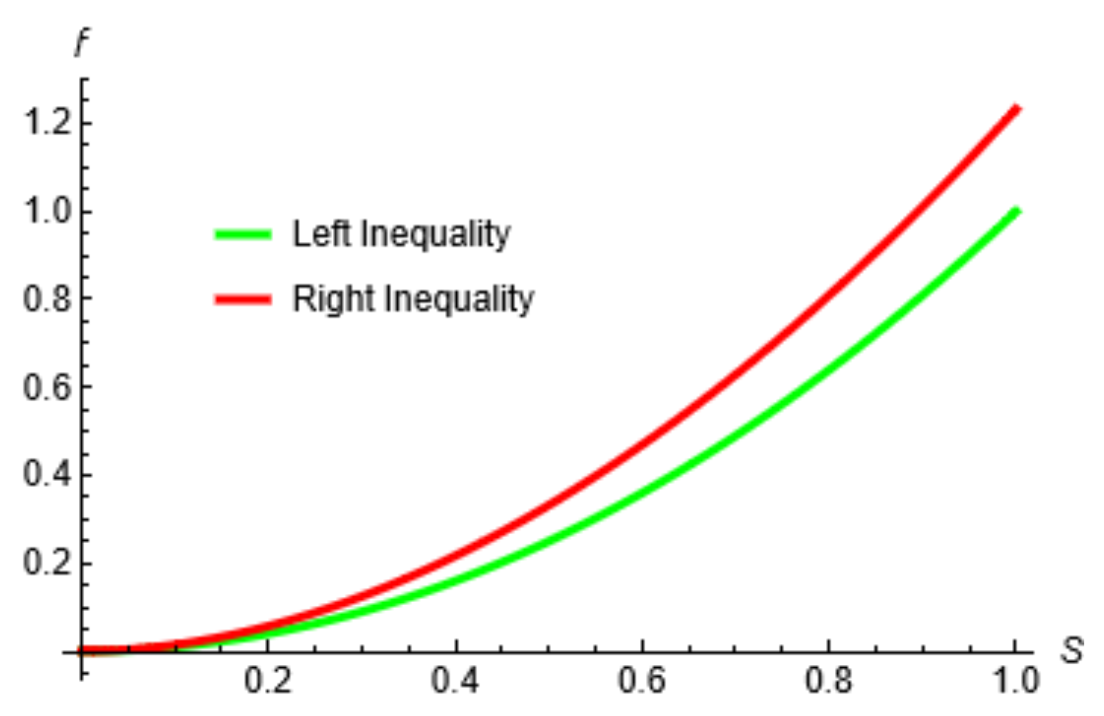
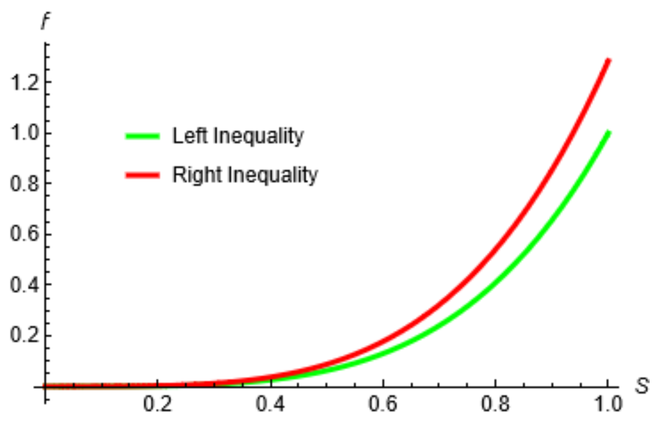
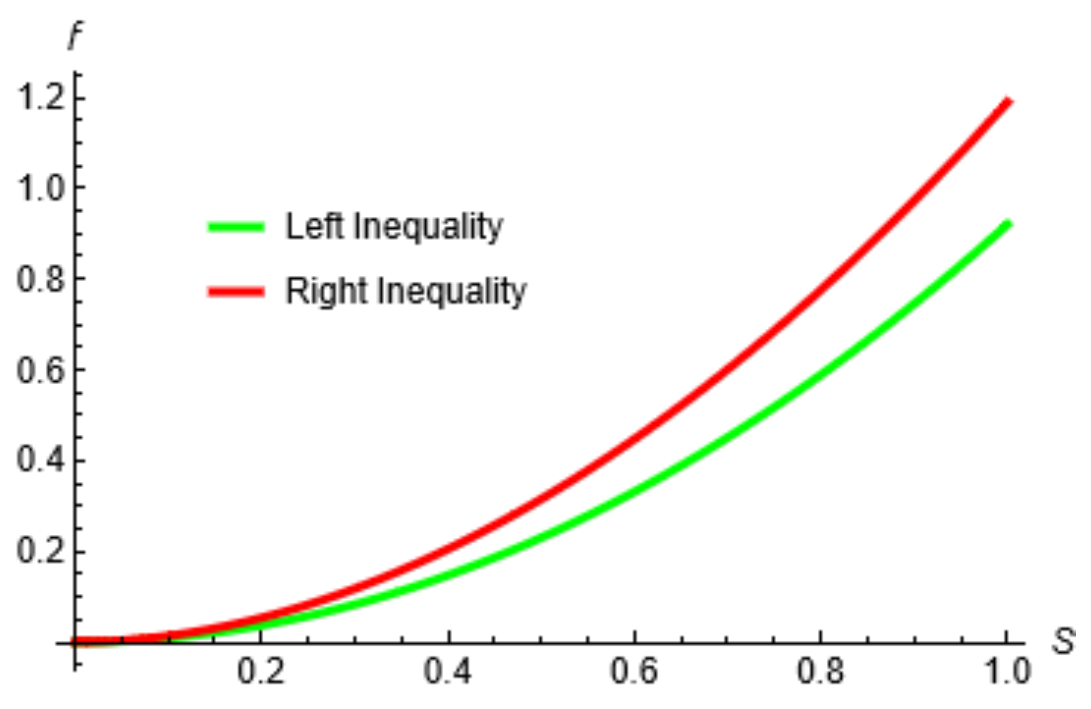
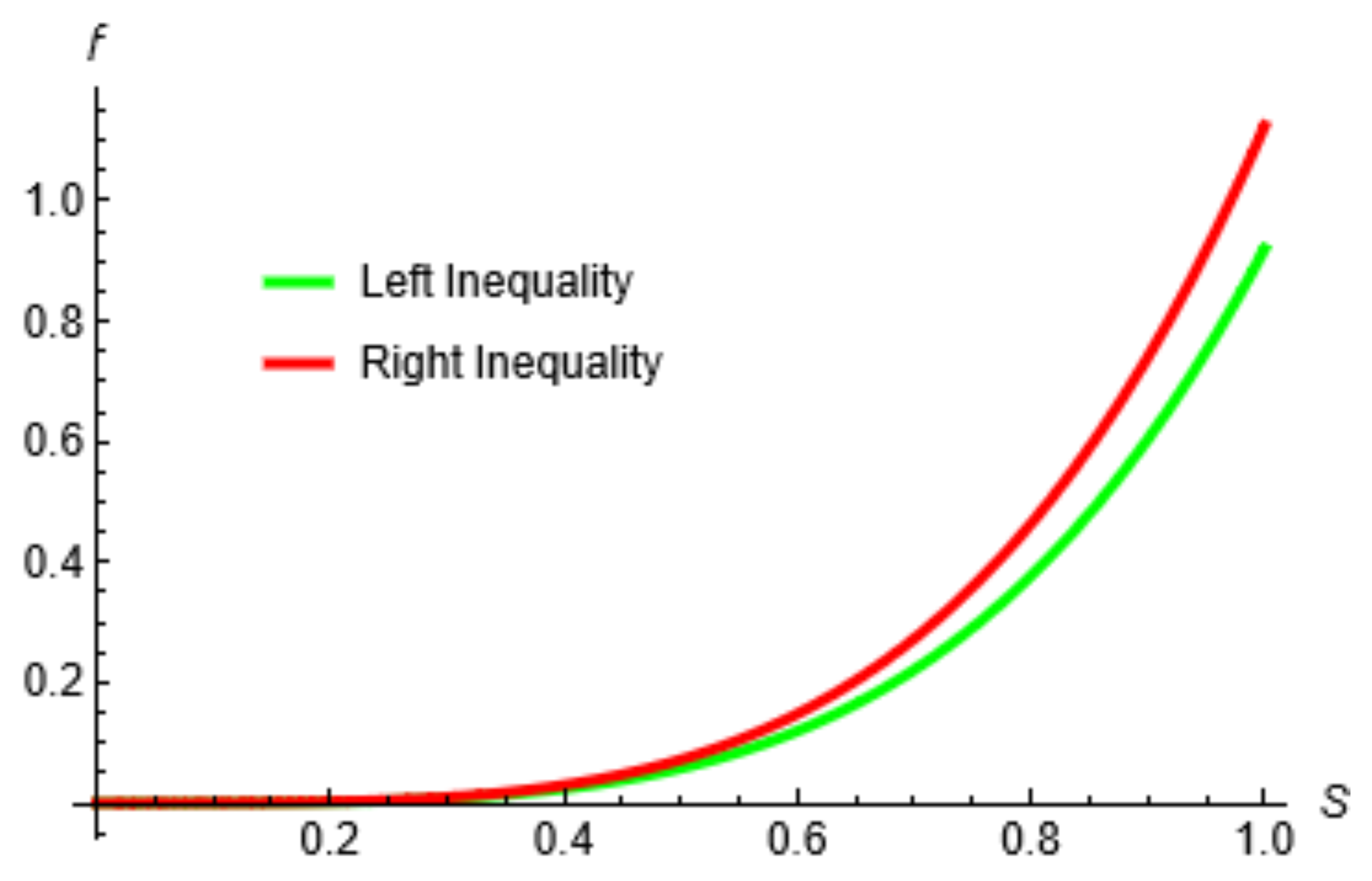
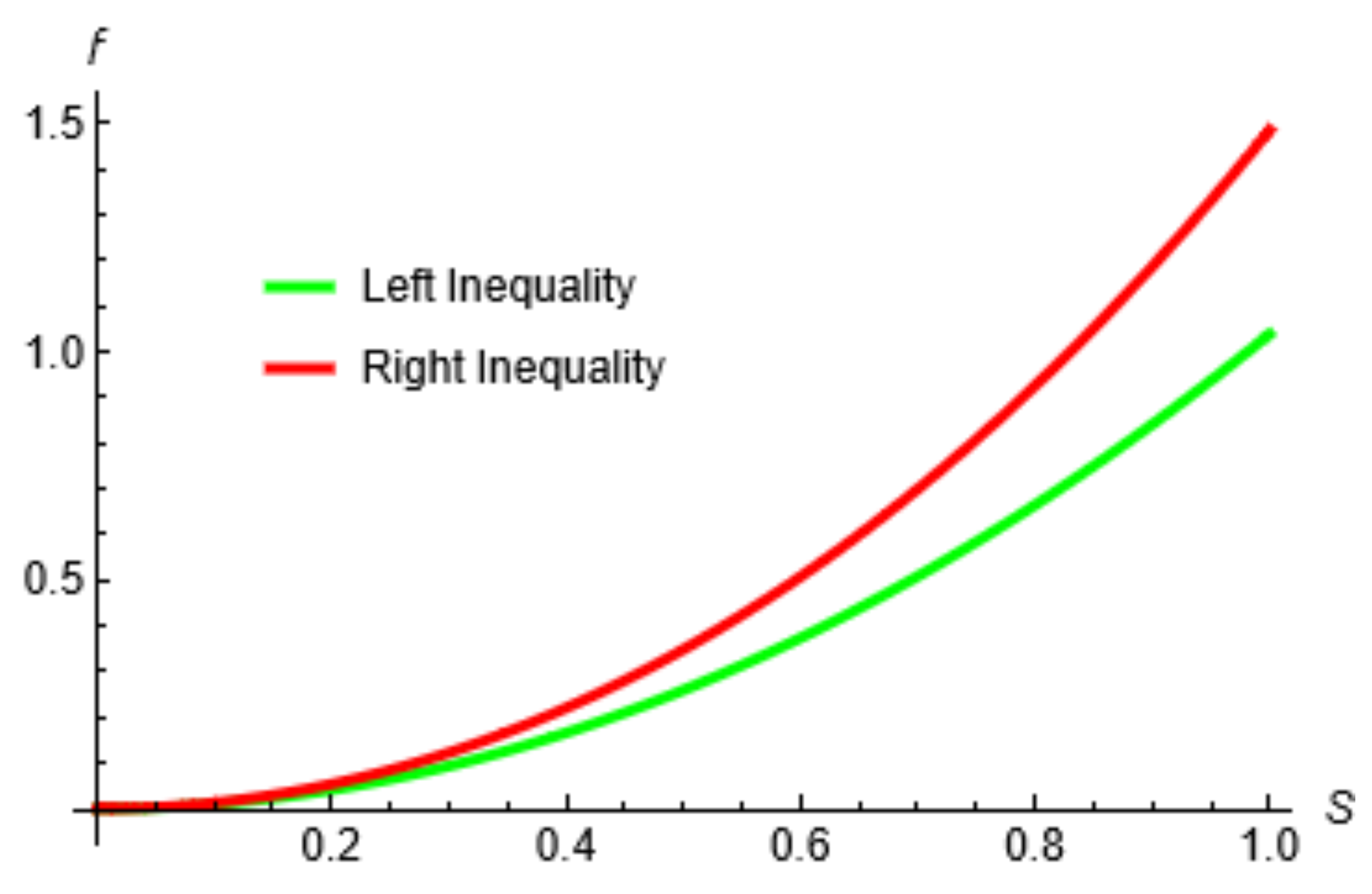
4. Numerical Examples and Their Computational Analysis

In this section, we give numerical examples and computational analysis of newly established results.

Example 1. 

Let $Ϝ:\left[{\theta }_1,{\theta }_2\right]=\left[1,2\right]\to {\mathbb{R}}^{+}$ be a function defined by $Ϝ\left(t\right)=t^2$. Moreover, for $s=\frac{1}{2}$, by applying inequality (11) to the function $Ϝ\left(t\right)=t^2$ we have

$$\begin{array}{ccc}\hfill {\left({\int }_1^2{\left(t^2\right)}^{dt}\right)}^{\frac{1}{{\theta }_2-{\theta }_1}}& =& 2.1654,\hfill \\ \hfill {\left[Ϝ\left({\theta }_1\right)Ϝ\left({\theta }_2\right){\left[Ϝ\left(\frac{{\theta }_1+{\theta }_2}{2}\right)\right]}^4\right]}^{\frac{1}{6}}& =& 2.1633,\hfill \end{array}$$

so, the left-hand side of (11) is

$$\left|\frac{{\left[Ϝ\left({\theta }_1\right)Ϝ\left({\theta }_2\right){\left[Ϝ\left(\frac{{\theta }_1+{\theta }_2}{2}\right)\right]}^4\right]}^{\frac{1}{6}}}{{\left({\int }_{{\theta }_1}^{{\theta }_2}{\left(Ϝ\left(\eta \right)\right)}^{d\eta }\right)}^{\frac{1}{{\theta }_2-{\theta }_1}}}\right|=0.9990,$$

(34)

and the right-hand side of (11) is

$${\left({Ϝ}^{\ast }\left({\theta }_1\right){Ϝ}^{\ast }\left({\theta }_2\right)\right)}^{\left({\theta }_2-{\theta }_1\right)\left(\frac{2^{-1-s}\times 3^{-2-s}\left(1-2^{2+s}\times 3^{1+s}-3^{2+s}+5^{2+s}+2^s\times 3^{1+s}s\right)}{2+3s+s^2}\right)}=1.3270.$$

(35)

From (34) and (35), it is clear that

$$0.9990<1.3270.$$

This confirm that inequality (11) proved in Theorem 6 is valid.

Example 2. 

Let $Ϝ:\left[{\theta }_1,{\theta }_2\right]=\left[1,2\right]\to {\mathbb{R}}^{+}$ be a function defined by $Ϝ\left(t\right)=t^2$. Moreover, for $s=\frac{1}{2}$, $p=2$ and $q=2,$ by applying inequality (16) to the function $Ϝ\left(t\right)=t^2$ the right-hand side of (16) is

$${\left({Ϝ}^{\ast }\left({\theta }_1\right){Ϝ}^{\ast }\left({\theta }_2\right)\right)}^{\frac{{\theta }_2-{\theta }_1}{2}\left(\frac{\left(2-2^{-s}\right)+2^{-s}}{s+1}\right){\left(\frac{2\left(1+2^{p+1}\right)}{6^{p+1}\left(p+1\right)}\right)}^{\frac{1}{p}}}=1.3502.$$

(36)

From (34) and (36), it is clear that

$$0.9990<1.3502.$$

This confirm that inequality (16) proved in Theorem 7 is valid.

Example 3. 

Let $Ϝ:\left[{\theta }_1,{\theta }_2\right]=\left[1,2\right]\to {\mathbb{R}}^{+}$ be a function defined by $Ϝ\left(t\right)=e^{t^2}$. Moreover, for $s=\frac{1}{2}$, $\varkappa =\frac{3}{2}$ and choose $M=2$; then, by applying inequality (22) to the function $Ϝ\left(t\right)=e^{t^2}$ we have

$$\begin{array}{ccc}\hfill {\left({\int }_1^2{\left(e^{t^2}\right)}^{dt}\right)}^{\frac{1}{{\theta }_2-{\theta }_1}}& =& e^{\frac{7}{3}},\hfill \\ \hfill Ϝ\left(t\right)& =& e^{\frac{9}{4}},\hfill \end{array}$$

so, the left-hand side of (22) is

$$\left|\frac{Ϝ\left(\varkappa \right)}{{\left({\int }_{{\theta }_1}^{{\theta }_2}{\left(Ϝ\left(\eta \right)\right)}^{d\eta }\right)}^{\frac{1}{{\theta }_2-{\theta }_1}}}\right|=0.9200,$$

(37)

and the right-hand side of (22) is

$$M^{\frac{1}{{\theta }_2-{\theta }_1}\left(\frac{{\left(\varkappa -{\theta }_1\right)}^2+{\left({\theta }_2-\varkappa \right)}^2}{s+1}\right)}=1.2599.$$

(38)

From (37) and (38), it is clear that

$$0.9200<1.2599.$$

This confirm that inequality (22) proved in Theorem 8 is valid.

Example 4. 

Let $Ϝ:\left[{\theta }_1,{\theta }_2\right]=\left[1,2\right]\to {\mathbb{R}}^{+}$ be a function defined by $Ϝ\left(t\right)=e^{t^2}$. Moreover, for $p=2$, $q=2$, $s=\frac{1}{2}$, $\varkappa =\frac{3}{4}$ and choose $M=\frac{3}{2}$; then, by applying inequality (24) to the function $Ϝ\left(t\right)=e^{t^2}$, the right-hand side of (24) is

$$M^{\frac{1}{{\left(1+p\right)}^{\frac{1}{p}}}{\left(\frac{2}{s+1}\right)}^{\frac{1}{q}}\left(\frac{{\left(\varkappa -{\theta }_1\right)}^2+{\left({\theta }_2-\varkappa \right)}^2}{{\theta }_2-{\theta }_1}\right)}=1.1447.$$

(39)

From (37) and (39), it is clear that

$$0.9200<1.1447.$$

This confirm that inequality (24) proved in Theorem 9 is valid.

Example 5. 

Let $Ϝ:\left[{\theta }_1,{\theta }_2\right]=\left[1,2\right]\to {\mathbb{R}}^{+}$ be a function defined by $Ϝ\left(t\right)=t^2$. Moreover, for $s=\frac{1}{2}$, $p=2$, $q=2$ and $\varkappa =\frac{3}{2}$; then, by applying inequality (30) to the function $Ϝ\left(t\right)=t^2,$ we have

$$\begin{array}{ccc}\hfill {\left({\int }_1^2{\left(t^2\right)}^{d\varkappa }\right)}^{\frac{1}{{\theta }_2-{\theta }_1}}& =& 2.1654,\hfill \\ \hfill Ϝ\left(\varkappa \right)& =& \frac{9}{4},\hfill \end{array}$$

so, the left-hand side of (30) is

$$\left|\frac{Ϝ\left(\varkappa \right)}{{\left({\int }_{{\theta }_1}^{{\theta }_2}{\left(Ϝ\left(\eta \right)\right)}^{d\eta }\right)}^{\frac{1}{{\theta }_2-{\theta }_1}}}\right|=1.0390,$$

(40)

and the right-hand side of (30) is

$${\left({\left({Ϝ}^{\ast }\left(\frac{\varkappa +{\theta }_1}{2}\right)\right)}^{{\left(\varkappa -{\theta }_1\right)}^2}{\left({Ϝ}^{\ast }\left(\frac{{\theta }_2+\varkappa }{2}\right)\right)}^{{\left({\theta }_2-\varkappa \right)}^2}\right)}^{\frac{2^{\frac{s-1}{q}}}{{\left(1+p\right)}^{\frac{1}{p}}\left({\theta }_2-{\theta }_1\right)}}=1.3902.$$

(41)

From (40) and (41), it is clear that

$$1.0390<1.3902.$$

This confirms that inequality (30) proved in Theorem 10 is valid.

Remark 5. 

To check the graphical behavior of newly established integrals inequalities, we need to vary the left parts of Theorems with respect to the right parts because we have a variation in right parts not in left parts; to overcome this difficulty, we multiply by $s^2$ on both sides of inequalities (11), (22) and (30), then multiply by $s^4$ on both sides of inequalities (16) and (24), respectively (Figure 1, Figure 2, Figure 3, Figure 4, Figure 5 and Table 1, Table 2, Table 3, Table 4, Table 5).

Figure 1. Depicts the comparative analysis between the left and right terms for discretization of “s” when inequality (11) is multiplied by $s^2$ in Theorem 6.

Figure 2. Depicts the comparative analysis between the left and right terms for discretization of “s” when inequality (16) is multiplied by $s^4$ in Theorem 7.

Figure 3. Depicts the comparative analysis between the left and right terms for discretization of “s” when inequality (22) is multiplied by $s^2$ in Theorem 8.

Figure 4. Depicts the comparative analysis between the left and right terms for discretization of “s” when inequality (24) is multiplied by $s^4$ in Theorem 9.

Figure 5. Depicts the comparative analysis between the left and right terms for discretization of “s” when inequality (30) is multiplied by $s^2$ in Theorem 10.

Table 1. Comparison between the left and right terms for discretization of “s” in Theorem 6.

s	Left Term	Right Term
0.2	0.0399	0.0568
0.4	0.1598	0.2166
0.6	0.3596	0.4692
0.8	0.6393	0.8087

Table 2. Comparison between the left and right terms for discretization of “s” in Theorem 7.

s	Left Term	Right Term
0.2	0.0015	0.0024
0.4	0.0255	0.0365
0.6	0.1294	0.1771
0.8	0.4092	0.5407

Table 3. Comparison between the left and right terms for discretization of “s” in Theorem 8.

s	Left Term	Right Term
0.2	0.0368	0.0533
0.4	0.1472	0.2049
0.6	0.3312	0.4470
0.8	0.5888	0.7758

Table 4. Comparison between the left and right terms for discretization of “s” in Theorem 9.

s	Left Term	Right Term
0.2	0.0014	0.0018
0.4	0.0235	0.0294
0.6	0.1192	0.1477
0.8	0.3768	0.4633

Table 5. Comparison between the left and right terms for discretization of “s” in Theorem 10.

s	Left Term	Right Term
0.2	0.0415	0.0540
0.4	0.1663	0.2207
0.6	0.3741	0.5081
0.8	0.6650	0.9260

5. Applications

In this section, we provide some applications to quadrature formula and special means for real numbers, to show the validity of the newly established inequalities for multiplicatively convex functions.

5.1. Applications to Quadrature Formula

In this subsection, for the first time, we provide an application to numerical integration in a multiplicative context for Simpson’s formula.

Let d be a partition of the points ${\theta }_1=u_0<u_1<u_2<....<u_{n-1}={\theta }_2$ of the interval $\left[{\theta }_1,{\theta }_2\right],$ and consider Simpson’s quadrature formula

$${\int }_{{\theta }_1}^{{\theta }_2}{\left(Ϝ\left(\eta \right)\right)}^{d\eta }=\left\{\begin{array}{c}R\left(Ϝ,d\right)\lambda \left(Ϝ,d\right),\lambda \left(Ϝ,d\right)\ge 0\\ \frac{R\left(Ϝ,d\right)}{\lambda \left(Ϝ,d\right)},\lambda \left(Ϝ,d\right)<0\end{array}\right.,$$

(42)

where

$$\begin{array}{ccc}& & \lambda \left(Ϝ,d\right)\hfill \\ & =& {\Pi }_{i=0}^{n-1}{\left(\left(Ϝ\left(u_i\right)\right)Ϝ{\left(\frac{u_i+u_{i+1}}{2}\right)}^4\left(Ϝ\left(u_{i+1}\right)\right)\right)}^{\frac{\left(u_{i+1}-u_i\right)}{6}},\hfill \end{array}$$

is the multiplicative Simpson version and the remainder term $R\left(Ϝ,d\right)$ satisfies the estimation

$$\left|R\left(Ϝ,d\right)\right|\le {\Pi }_{i=0}^{n-1}{\left[{Ϝ}^{\ast }\left(u_i\right){Ϝ}^{\ast }\left(u_{i+1}\right)\right]}^{\frac{5{\left(u_{i+1}-u_i\right)}^2}{72}}.$$

Now, we derive some error estimates for Simpson’s formula.

Proposition 2. 

Let $Ϝ:\left[{\theta }_1,{\theta }_2\right]\subset \mathbb{R}\to {\mathbb{R}}^{+}$ be *differentiable function on $\left({\theta }_1,{\theta }_2\right).$ If ${Ϝ}^{\ast }$ is a multiplicatively s-convex function in the second sense on $\left[{\theta }_1,{\theta }_2\right]$ for some fixed $s\in \left(0,1\right]$ then in (42) for every division d of $\left[{\theta }_1,{\theta }_2\right]$ we have

$$\left|R\left(Ϝ,d\right)\right|\le {\Pi }_{i=0}^{n-1}{\left[{Ϝ}^{\ast }\left(u_i\right){Ϝ}^{\ast }\left(u_{i+1}\right)\right]}^{\frac{5{\left(u_{i+1}-u_i\right)}^2}{72}}.$$

(43)

Proof. 

Applying Theorem 6 on the subinterval $\left[u_i,u_{i+1}\right]$ of the division d, we obtain

$$\begin{array}{ccc}& & \left|\frac{{\int }_{u_i}^{u_{i+1}}{\left(Ϝ\left(u\right)\right)}^{du}}{{\left(\left(Ϝ\left(u_i\right)\right)Ϝ{\left(\frac{u_i+u_{i+1}}{2}\right)}^4\left(Ϝ\left(u_{i+1}\right)\right)\right)}^{\frac{\left(u_{i+1}-u_i\right)}{6}}}\right|\hfill \\ & \le & {\left({Ϝ}^{\ast }\left(u_i\right){Ϝ}^{\ast }\left(u_{i+1}\right)\right)}^{{\left(u_{i+1}-u_i\right)}^2\left(\frac{2^{-1-s}\times 3^{-2-s}\left(1-2^{2+s}\times 3^{1+s}-3^{2+s}+5^{2+s}+2^s\times 3^{1+s}s\right)}{2+3s+s^2}\right)},\hfill \end{array}$$

where $h_i=\frac{u_{i+1}-u_i}{2},$$i=0,1,2,....,n-1$. Hence, we have

$$\begin{array}{cc}\hfill & \left|\frac{{\int }_{{\theta }_1}^{{\theta }_2}{\left(Ϝ\left(u\right)\right)}^{du}}{\lambda \left(Ϝ,d\right)}\right|\hfill \\ \hfill & =\left|{\Pi }_{i=0}^{n-1}\frac{{\int }_{u_i}^{u_{i+1}}{\left(Ϝ\left(u\right)\right)}^{du}}{{\left(\left(Ϝ\left(u_i\right)\right)Ϝ{\left(\frac{u_i+u_{i+1}}{2}\right)}^4\left(Ϝ\left(u_{i+1}\right)\right)\right)}^{\frac{\left(u_{i+1}-u_i\right)}{6}}}\right|\hfill \\ \hfill & \le {\Pi }_{i=0}^{n-1}\left|\frac{{\int }_{u_i}^{u_{i+1}}{\left(Ϝ\left(u\right)\right)}^{du}}{{\left(\left(Ϝ\left(u_i\right)\right)Ϝ{\left(\frac{u_i+u_{i+1}}{2}\right)}^4\left(Ϝ\left(u_{i+1}\right)\right)\right)}^{\frac{\left(u_{i+1}-u_i\right)}{6}}}\right|\hfill \\ \hfill & \le {\Pi }_{i=0}^{n-1}{\left[{Ϝ}^{\ast }\left(u_i\right){Ϝ}^{\ast }\left(u_{i+1}\right)\right]}^{{\left(u_{i+1}-u_i\right)}^2\left(\frac{2^{-1-s}\times 3^{-2-s}\left(1-2^{2+s}\times 3^{1+s}-3^{2+s}+5^{2+s}+2^s\times 3^{1+s}s\right)}{2+3s+s^2}\right)}.\hfill \end{array}$$

(44)

For instance, if $s=1$ in (44), then we have

$$\begin{array}{ccc}& & \left|\frac{{\int }_{{\theta }_1}^{{\theta }_2}{\left(Ϝ\left(u\right)\right)}^{du}}{\lambda \left(Ϝ,d\right)}\right|\hfill \\ & \le & {\Pi }_{i=0}^{n-1}{\left[{Ϝ}^{\ast }\left(u_i\right){Ϝ}^{\ast }\left(u_{i+1}\right)\right]}^{\frac{5{\left(u_{i+1}-u_i\right)}^2}{72}}.\hfill \end{array}$$

This completes the proof. □

Proposition 3. 

Let $Ϝ:\left[{\theta }_1,{\theta }_2\right]\subset \mathbb{R}\to {\mathbb{R}}^{+}$ be *differentiable function on $\left({\theta }_1,{\theta }_2\right).$ If $\left(ln({Ϝ}^{\ast }\right){)}^q$ is a multiplicatively s-convex function in the second sense on $\left[{\theta }_1,{\theta }_2\right]$ for some fixed $s\in \left(0,1\right]$ then in (42) for every division d of $\left[{\theta }_1,{\theta }_2\right]$ we have

$$\begin{array}{ccc}& & \left|R\left(Ϝ,d\right)\right|\hfill \\ & \le & {\Pi }_{i=0}^{n-1}{\left[{Ϝ}^{\ast }\left(u_i\right){Ϝ}^{\ast }\left(u_{i+1}\right)\right]}^{\frac{{\theta }_2-{\theta }_1}{2}\left(\frac{\left(2-2^{-s}\right)+2^{-s}}{s+1}\right){\left(\frac{2\left(1+2^{p+1}\right)}{6^{p+1}\left(p+1\right)}\right)}^{\frac{1}{p}}}.\hfill \end{array}$$

Proof. 

With the help of Theorem 7 the proof is similar to Proposition 2. □

Remark 6. 

In a similar way, one can obtain more results for a midpoint-type inequality.

Remark 7. 

The classical error estimates based on Taylor expansion for the Simpson formula involve the 4th derivative ${\left|\left|{Ϝ}^{\left(4\right)}\right|\right|}_{\infty }$. In the case that the ${Ϝ}^{\left(4\right)}$ derivative does not exist or is very large at some points in $\left[{\theta }_1,{\theta }_2\right]$ the classical estimates cannot be applied and, thus, ref. (43) provides an alternative approximation for the Simpson formula. This is a new approach in multiplicative calculus.

5.2. Applications to Special Means of Real Numbers

In this section of the paper, we will consider the following special means for real numbers ${\theta }_1,{\theta }_2$ with ${\theta }_1\ne {\theta }_2$. We have

(1) The arithmetric means for ${\theta }_1,{\theta }_2\in {\mathbb{R}}^{+}$: $A\left({\theta }_1,{\theta }_2\right)=\frac{{\theta }_1+{\theta }_2}{2}$.

(2) The geometric means for ${\theta }_1,{\theta }_2\in {\mathbb{R}}^{+}$: $G\left({\theta }_1,{\theta }_2\right)=\sqrt{{\theta }_1{\theta }_2}$.

(3) The harmonic means for ${\theta }_1,{\theta }_2\in {\mathbb{R}}^{+}\setminus \left\{0\right\}$: $H\left({\theta }_1,{\theta }_2\right)=\frac{2{\theta }_1{\theta }_2}{{\theta }_1+{\theta }_2}$.

(4) The logarithmic means for ${\theta }_1,{\theta }_2\in {\mathbb{R}}^{+}$ and $\left|{\theta }_1\right|\ne \left|{\theta }_2\right|$: $L\left({\theta }_1.{\theta }_2\right)=\frac{{\theta }_1-{\theta }_2}{ln\left|{\theta }_2\right|-ln\left|{\theta }_1\right|}$.

(5) The identric means for ${\theta }_1,{\theta }_2\in {\mathbb{R}}^{+}\setminus \left\{0\right\}$: $I\left({\theta }_1,{\theta }_2\right):=\left\{\begin{array}{c}\frac{1}{e}{\left(\frac{{\theta }_2^{{\theta }_2}}{{\theta }_1^{{\theta }_1}}\right)}^{\frac{1}{{\theta }_2-{\theta }_1}},{\theta }_1\ne {\theta }_2\\ {\theta }_1,{\theta }_1={\theta }_2\end{array}\right.$.

(6) The generalized logarithmic means for ${\theta }_1,{\theta }_2\in \mathbb{R}\setminus \left\{0\right\}$ and $n\in \mathbb{R}\setminus \left\{-1,0\right\}$: $L_p\left({\theta }_1,{\theta }_2\right)={\left[\frac{{\theta }_2^{n+1}-{\theta }_1^{n+1}}{\left(n+1\right)\left({\theta }_2-{\theta }_1\right)}\right]}^{\frac{1}{m}}$.

Proposition 4. 

Suppose ${\theta }_1,{\theta }_2\in {\mathbb{R}}^{+}$ with $0<{\theta }_1<{\theta }_2$; then, we have

$$\begin{array}{ccc}& & {\left(e^{A\left({\theta }_1^{n+1},{\theta }_2^{n+1}\right)+A^{n+1}-3L_{n+1}^{n+1}\left({\theta }_1,{\theta }_2\right)}\right)}^{\frac{1}{3\left(n+1\right)}}\hfill \\ & \le & {\left(e^{nA\left({\theta }_1^{n-1},{\theta }_2^{n-1}\right)}\right)}^{\left({\theta }_2-{\theta }_1\right){\left(\frac{2\left(1+2^{p+1}\right)}{6^{p+1}\left(p+1\right)}\right)}^{\frac{1}{p}}}.\hfill \end{array}$$

Proof. 

The assertion follows from Corollary 2, applied to the function $Ϝ\left(t\right)=e^{t^n}$ with $n\ge 2$ whose ${\left({\int }_{{\theta }_1}^{{\theta }_2}{\left(Ϝ\left(t\right)\right)}^{dt}\right)}^{\frac{1}{{\theta }_2-{\theta }_1}}=e^{\frac{1}{{\theta }_2-{\theta }_1}{\int }_{{\theta }_1}^{{\theta }_2}ln{e}^{t^n}dt}=e^{L_n^n\left({\theta }_1,{\theta }_2\right)}$ and ${Ϝ}^{\ast }\left(t\right)=e^{n{t}^{n-1}}.$ □

Proposition 5. 

Suppose ${\theta }_1,{\theta }_2\in {\mathbb{R}}^{+}$ with $0<{\theta }_1<{\theta }_2$; then, we have

$$\frac{e^{{\varkappa }^n}}{e^{L_n^n\left({\theta }_1,{\theta }_2\right)}}\le M^{\frac{1}{{\theta }_2-{\theta }_1}\left(\frac{{\left(\varkappa -{\theta }_1\right)}^2+{\left({\theta }_2-\varkappa \right)}^2}{2}\right)}.$$

(45)

Proof. 

If $Ϝ\left(t\right)=e^{t^n}$ with $n\ge 1$ then we have ${\left({\int }_{{\theta }_1}^{{\theta }_2}{\left(Ϝ\left(t\right)\right)}^{dt}\right)}^{\frac{1}{{\theta }_2-{\theta }_1}}=e^{L_n^n\left({\theta }_1,{\theta }_2\right)}$, from Corollary 4, and we have following relation for $M=e^{n{b}^{n-1}}$. For more instances, if we put

(i) $\varkappa =A$ in (45) then we have

$$e^{{\varkappa }^n-L_n^n}\le M^{\frac{1}{{\theta }_2-{\theta }_1}\left(\frac{{\left(A-{\theta }_1\right)}^2+{\left({\theta }_2-A\right)}^2}{2}\right)}.$$

(ii) One can write similar inequalities by choosing $\varkappa =G,H,L,I$. □

Proposition 6. 

Suppose ${\theta }_1,{\theta }_2\in {\mathbb{R}}^{+}$ with $0<{\theta }_1<{\theta }_2$; then, we have

$$\frac{e^{{\varkappa }^{n+1}}}{e^{L_{n+1}^{n+1}\left({\theta }_1,{\theta }_2\right)}}\le M^{\frac{1}{{\left(1+p\right)}^{\frac{1}{p}}}\left(\frac{{\left(\varkappa -{\theta }_1\right)}^2+{\left({\theta }_2-\varkappa \right)}^2}{{\theta }_2-{\theta }_1}\right)}.$$

(46)

Proof. 

If $Ϝ\left(t\right)=e^{\frac{1}{n+1}{t}^{n+1}}$ with $n\ge 1$ then ${Ϝ}^{\ast }\left(t\right)=e^{t^n}$ is multiplicatively convex on a given interval and we have ${\left({\int }_{{\theta }_1}^{{\theta }_2}{\left(Ϝ\left(t\right)\right)}^{dt}\right)}^{\frac{1}{{\theta }_2-{\theta }_1}}=e^{\frac{1}{n+1}{L}_{n+1}^{n+1}\left({\theta }_1,{\theta }_2\right)}$, from Corollary 6, and we have obtained inequality (46). For more instances, if we put

(i) $\varkappa =A$ in (46) then we have

$$e^{{\varkappa }^n-L_{n+1}^{n+1}}\le M^{\frac{1}{{\left(1+p\right)}^{\frac{1}{p}}}\left(\frac{{\left(A-{\theta }_1\right)}^2+{\left({\theta }_2-A\right)}^2}{{\theta }_2-{\theta }_1}\right)}.$$

(ii) One can write similar inequalities by choosing $\varkappa =G,H,L,I$. □

6. Conclusions

This paper’s aim was to establish some generalized integral inequalities for multiplicatively differentiable convex functions. We established integral inequalities of the Simpson and Ostrowski types for s-convex functions in the second sense within the framework of multiplicative calculus. In addition, we gave the numerical examples and computational analysis to examine the behavior of newly established inequalities for multiplicatively s-convex functions in the second sense. Applications to quadrature formula and special means of real numbers by utilizing our newly established results were also given. The results in this paper should be very interesting and innovative in the field of multiplicative calculus and inequalities. These generalizations will be helpful for researchers working in the field of mathematical modeling, optimization and numerical analysis. Interested readers could establish several new results in this field by using our new ideas.

References

1. Mitrinovic, D.S.; Pecaric, J.; Fink, A.N. Inequalities Involving Functions and Their Integrals and Derivatives; Springer Science & Business Media: Berlin/Heidelberg, Germany, 1991; Volume 53. [Google Scholar]
2. Ali, M.A.; Mateen, A.; Feckan, M. Study of Quantum Ostrowski’s-Type Inequalities for Differentiable convex Functions. Ukr. Math. J. 2023, 75, 7–27. [Google Scholar] [CrossRef]
3. Pachpatte, B.G. On an inequality of Ostrowski’s type in three independent variables. J. Math. Anal. Appl. 2000, 249, 583–591. [Google Scholar] [CrossRef]
4. Budak, H.; Tunç, T.; Sarikaya, M.Z. Fractional Hermite-Hadamard type inequalities for interval valued functions. Proc. Am. Math. Soc. 2020, 148, 705–718. [Google Scholar] [CrossRef]
5. Daletskii, Y.L.; Teterina, N.I. Multiplicative stochastic integrals. Uspekhi Mat. Nauk 1972, 27, 167–168. [Google Scholar]
6. Ali, M.A.; Budak, H.; Sarikaya, M.Z.; Zhang, Z. Ostrowski and Simpson type inequalities for multiplicative integrals. Proyecciones 2021, 40, 743–763. [Google Scholar] [CrossRef]
7. Bashirov, A.E.; Riza, M. On complex multiplicative differentiation. TWMS J. Appl. Eng. Math. 2011, 1, 75–85. [Google Scholar]
8. Özcan, S. Some Integral Inequalities of Hermite-Hadamard Type for Multiplicatively s-Preinvex Functions. Int. J. Math. Model. Comput. 2019, 9, 253–266. [Google Scholar] [CrossRef]
9. Dragomir, S.S.; Fitzpatrick, S. The Hadamard’s inequality for s-convex functions in the second sense. Demonstr. Math. 1999, 32, 687–696. [Google Scholar]
10. Sarikaya, M.Z.; Set, E.; Ozdemir, M.E. On new inequalities of Simpson’s type for s-convex functions. Appl. Math. Comput. 2010, 60, 2191–2199. [Google Scholar] [CrossRef]
11. Khan, S.; Budak, H. On midpoint and trapezoidal type inequalities for multiplicative integral. Mathematica 2017, 59, 124–133. [Google Scholar]
12. Özcan, S. Hermite-Hadamard type ınequalities for multiplicatively s-convex functions. Cumhur. Sci. J. 2020, 41, 245–259. [Google Scholar] [CrossRef]
13. Özyapici, A.; Misirli, E. Exponential approximation on multiplicative calculus. In Proceedings of the 6th ISAAC Congress, Ankara, Turkey, 13–18 August 2007; p. 471. [Google Scholar]
14. Breckner, W.W. Stetigkeitsaussagen füreine Klasse verallgemeinerter konvexer funktionen in topologischen lin-earen Räumen. Publ. Inst. Math. 1978, 23, 13–20. [Google Scholar]
15. Hudzik, H.; Maligranda, L. Some remarks on s-convex functions. Aequationes Math. 1994, 4, 100–111. [Google Scholar] [CrossRef]
16. Pycia, M. A direct proof of the s-Hölder continuity of Breckner s-convex functions. Aequationes Math. 2001, 61, 128–130. [Google Scholar] [CrossRef]
17. Ali, M.A.; Kara, H.; Tariboon, J.; Asawasamrit, S.; Budak, H.; Hezenci, F. Some new Simpson’s formula-type inequalities for twice-differentiable convex functions via generalized fractional operators. Symmetry 2021, 13, 2249. [Google Scholar] [CrossRef]
18. Meftah, B. Some new Ostrowski’s inequalities for functions whose nth derivatives are logarithmically convex. Ann. Math. Sil. 2017, 32, 275–284. [Google Scholar] [CrossRef]
19. Rangel-Oliveros, Y.; Nwaeze, E.R. Simpson’s type inequalities for exponentially convex functions with applications. Open J. Math. Sci. 2021, 5, 84–94. [Google Scholar] [CrossRef]
20. Mateen, A.; Zhang, Z.; Ali, M.A.; Feckan, M. Generalization of some integral inequalities in multiplicative calculus with their computational analysis. Ukr. Math. J. 2023. [Google Scholar] [CrossRef]
21. Grossman, M.; Katz, R. Non-Newtonian Calculus; Lee Press: Pigeon Cove, MA, USA, 1972. [Google Scholar]
22. Aniszewska, D. Multiplicative runge-Kutta methods. Nonlinear Dyn. 2007, 50, 265–272. [Google Scholar] [CrossRef]
23. Riza, M.; Özyapici, A.; Misirli, E. Multiplicative finite difference methods. Q. Appl. Math. 2009, 67, 745–754. [Google Scholar] [CrossRef]
24. Bhat, A.H.; Majid, J.; Shah, T.R.; Wani, I.A.; Jain, R. Multiplicative Fourier transform and its applications to multiplicative differential equations. J. Comput. Math. Sci. 2019, 10, 375–383. [Google Scholar] [CrossRef]
25. Bhat, A.H.; Majid, J.; Wani, I.A. Multiplicative Sumudu transform and its Applications. Emerg. Technol. Innov. Res. 2019, 6, 579–589. [Google Scholar]
26. Misirli, E.; Gurefe, Y. Multiplicative Adams Bashforth-Moulton methods. Numer. Algorithms 2011, 57, 425–439. [Google Scholar] [CrossRef]
27. Chasreechai, S.; Ali, M.A.; Naowarat, S.; Sitthiwirattham, T.; Nonlaopon, K. On Some Simpson’s and Newton’s Type Inequalities in Multiplicative Calculus with Applications. AIMS Math. 2023, 8, 3885–3896. [Google Scholar] [CrossRef]
28. Bashirov, A.E. On line and double multiplicative integrals. TWMS J. Appl. Eng. Math. 2013, 3, 103–107. [Google Scholar]
29. Xi, B.-Y.; Qi, F. Some integral inequalities of Hermite-Hadamard type for s-logarithmically convex functions. Acta Math. Sci. Engl. Ser. 2015, 35A, 515–526. [Google Scholar]
30. Bai, Y.M.; Qi, F. Some integral inequalities of the Hermite-Hadamard type for log-convex functions on co-ordinates. J. Nonlinear Sci. 2016, 9, 5900–5908. [Google Scholar] [CrossRef]
31. Dragomir, S.S. Further inequalities for log-convex functions related to Hermite-Hadamard result. Proyecciones 2019, 38, 267–293. [Google Scholar] [CrossRef]
32. Set, E.; Ardiç, M.A. Inequalities for log-convex functions and p-function. Miskolc Math. Notes 2017, 18, 1033–1041. [Google Scholar] [CrossRef]
33. Zhang, X.M.; Jiang, W.D. Some properties of log-convex function and applications for the exponential function. Comput. Math. Appl. 2012, 63, 1111–1116. [Google Scholar] [CrossRef]
34. Bashirov, A.E.; Kurpınar, E.M.; Özyapıcı, A. Multiplicative calculus and its applications. J. Math. Anal. Appl. 2008, 337, 36–48. [Google Scholar] [CrossRef]
35. Ali, M.A.; Abbas, M.; Zhang, Z.; Sial, I.B.; Arif, R. On integral inequalities for product and quotient of two multiplicatively convex functions. Asian Res. J. Math. 2019, 12, 1–11. [Google Scholar] [CrossRef]