Impact of Capital Position and Financing Strategies on Encroachment in Supply Chain Dynamics

Abstract

Channel encroachment and financing decisions are prevalent in practice. Utilizing the Stackelberg game framework, we investigate the impact of a retailer’s capital position and financing strategies on supply chain dynamics in which a supplier considers establishing a direct sales channel. We find that the retailer’s equilibrium financing strategy is impacted by demand volatility and the initial working capital. The supplier’s encroachment decision hinges on the entry cost when neither trade credit financing nor bank credit financing is available. When both types of credit are available, the choice of financing is a complex interplay involving initial working capital, entry cost, and demand volatility. Notably, the supplier’s decision to encroach may shift from a binary stance of either encroaching or not encroaching, or it may oscillate from encroachment to non-encroachment and back to encroachment, particularly with an increase in demand volatility when the entry cost is moderate. The novelty of this study lies in its integration of supplier channel decisions with retailer operational decisions and financing strategies, examining how the capital position and financing strategies impact channel decisions. This study provides managerial insights into the interplay between supplier’s channel dynamics and retailer’s financial considerations, shedding light on unexplored aspects of channel management. In future studies, some assumptions in this study can be modified to obtain more managerial insights.

1. Introduction

Online sales in US retail jumped 40% year over year in 2021. In 2023, about 27.6% of the total retail sales in China were made online. The rapid growth of online sales has prompted numerous suppliers to embrace online channels and actively engage in the consumer market. Examples include prominent suppliers in the electronics sector such as HP, Apple, Dell, and Huawei, as well as flourishing entities in the clothing and fashion accessories sector like Gucci, Adidas, Nike, and Coach. The practice that suppliers have established direct sales channels as an addition to their existing retail networks is referred to as supplier encroachment [1]. This strategic expansion into the retail sector is increasingly acknowledged as a crucial approach for boosting supplier’s profitability. Moreover, the evolution of information technology and the rise of e-commerce have significantly facilitated the expansion into new sales channels, making it increasingly accessible and cost-effective for upstream suppliers. For example, through digital channels, many companies in the US are exploring ways to reach consumers directly, looking to engage consumers in highly personalized, consistent interactions (https://www.mckinsey.com/industries/consumer-packaged-goods/our-insights/should-cpg-manufacturers-go-direct-to-consumer-and-if-so-how, accessed on 10 March 2024). However, the suppliers’ choice to directly engage with consumers may result in displeasing their retail partners. Specially, the encroaching suppliers can not only charge a wholesale price but can also compete with the downstream retailers, posing a real threat to the retailers and resulting in channel conflicts [2]. Therefore, the suppliers’ strategy of encroachment must be incorporated into a comprehensive channel strategy that anticipates and effectively resolves potential channel conflicts.

Trade credit is an important practice in the supply chain for mitigating channel conflicts [3,4]. In addition, suppliers are more inclined to participate in the end consumer market when downstream retailers are financially constrained. For example, Gree, a famous Chinese air conditioner company and one of the world’s top 500 companies, not only provided financing policies (extending the account period; flexible payment policies) for downstream retailers, but also actively participated in sales through online channels. Similarly, car manufacturers (e.g., Geely) provided trade credit financing to dealers and launched direct sales channels in order to ease the pressure on auto dealers and promote consumption, (e.g., Zeekr) [5]. In practice, downstream retailers often encounter constraints in their working capital for day-to-day operations [6,7]. The issue of capital shortages poses a significant challenge for small and medium-sized enterprises (SMEs) worldwide. Over 40 million SMEs in China are struggling with a lack of working capital, requiring prompt financial intervention [8]. Typically, firms facing capital constraints turn to two primary sources of financing support: bank credit and trade credit. Based on data from the Small Firms Lending Index published by Forbes, 22.8% of small firms accessed bank credit in 2015 [9]. Concurrently, many corporations expand the use of trade credit [10].

Motivated by the above discussion, we aim to study the supplier’s encroaching decision and the retailer’s financing choice when both trade credit and bank credit options are available. We study the interplay between the supplier’s encroaching decision and the retailer’s financing strategy, considering the retailer’s initial working capital. It is assumed that the retailer has the first-mover advantage in the credit market because the financial market, including bank and trade credit financing, is usually supposed to be competitive in the related literature [11,12,13]. Specifically, we investigate the following questions: (1) What is the supplier’s decision regarding encroachment when credit financing is not available, and when both types of credit financing are available? (2) What is the financing equilibrium when both trade credit and bank credit financing are available to the retailer without supplier encroachment? (3) When both trade credit and bank credit financing are available, what is the financing equilibrium with supplier encroachment? (4) What effects does supplier encroachment have on operational decisions and the retailer’s payoff?

To answer the above questions, we study a two-level decentralized supply chain where a retailer with limited initial capital purchases products from a supplier. The demand is uncertain and price-sensitive, as indicated by a linear downward-sloping inverse demand function. The sequence of events unfolds through a three-stage game. First, the supplier determines the wholesale price and makes an encroaching decision with commitment. The policy is established in advance to allow the supplier to prepare for setting up the new direct sales channel [14,15,16]. This includes establishing company-owned franchises, outlets, and online websites, as well as recruiting and training a sales force. Second, the retailer decides on the financing option and the order quantity. Third, the supplier determines the amount of encroachment. Apart from production, the supplier may also enter the retail market to gain an advantage by posing a threat to the retailer. This would allow the supplier to set more flexible prices and control the market distribution. However, the supplier may choose not to enter the retail market because the success of such a move depends on various factors, leading to hesitation in establishing a direct sales channel. Therefore, the supplier’s decision for encroachment is unclear and needs to be studied.

Since supplier encroachment and credit financing in practical scenarios often coexist, we have incorporated the examination of supplier encroachment into our analysis of credit financing. We make the following contributions. First, our study offers a distinctive operational perspective that complements the existing literature by addressing the intertwined dynamics of supplier encroachment and credit financing while considering the retailer’s initial working capital. Second, we contribute novel insights by calculating the thresholds of a retailer’s initial working capital under different scenarios where the retailer is capital-constrained or capital-sufficient. This analytical approach offers practical guidance for retailers in determining the optimal operational strategies based on their financial constraints. Third, we reveal nuanced patterns in supplier encroachment decisions under varying conditions. Specifically, our findings highlight the binary nature of supplier encroachment decisions, which may transition from encroachment to no encroachment and then back to encroachment in response to the change in demand volatility, particularly when entry costs are moderate.

The rest of the paper is as follows. Section 2 provides a summary of the related literature. Section 3 introduces the model assumptions and settings. Section 4 examines the equilibria under trade credit financing and bank credit financing. The impacts of financing strategies and supplier encroachment are analyzed in Section 5. Finally, Section 6 presents the conclusion, including the main findings, managerial implications, and future scope, with all proofs given in Appendix A.

2. Literature Review

Our study relates to two main streams in the literature: supplier encroachment and trade credit financing. First, this study is related to the emerging research on supplier encroachment. The conventional perspective shows that upstream supplier encroachment could potentially undermine the interests of retailers, as the implementation of a supplier’s direct sales channel results in competition within the supply chain distribution. However, some recent studies have identified that supply encroachment could benefit both the supplier and the retailer [17,18,19,20,21]. Specifically, Cao and Qin [22] demonstrated that the encroaching supplier and the target-oriented retailer can achieve a win-win situation when a retailer’s target and demand variability are low. Liang et al. [23] extended this research and illustrated that encroachment can enhance the total profit for both the manufacturer and the retailer with external options. Elahi et al. [24] discovered a scenario where both suppliers and retailers can simultaneously profit from the supplier’s capacity constraints. Ghosh et al. [25] showed that a dual-channel model could be coordinated and the retailer’s profit could be improved through sharing the cooperative advertising costs and adopting a return policy. In addition, many scholars also have conducted in-depth research on the factors influencing suppliers’ encroaching decisions. Within an intuitionistic type-2 fuzzy framework, Bhunia et al. [26] proposed a multi-period closed-loop retailing strategy for consumer services incorporating carbon cap and trade policy. Maruthasalam and Balasubramanian [27] demonstrated that minor asymmetric competition among retailers has positive impacts on supplier encroachment. Zhang et al. [28] studied the comprehensive impacts of product quality, information decisions, and sales costs on encroachment decisions and found that the manufacturer and the retailer can achieve a win-win situation through encroachment with moderate selling costs. Furthermore, some scholars have sought solutions to anti-encroachment. Zhang et al. [29] proposed that retail service investing may be an effective anti-encroachment strategy for the dominant retailer with highly efficient service investing. Yao et al. [30] suggested that the retailer’s strategic pricing could serve as a novel and cost-free anti-encroachment device. Zhang et al. [5] studied the interaction between the channel’s power structure and the retailer’s financing choice and illustrated that the capital-constrained retailer may deter the manufacturer’s encroachment behavior by choosing trade credit financing.

Second, this study also complements the extensive literature on trade credit financing in supply chains [11,12,13,31,32,33,34,35]. Specifically, Alan and Gaur [36] investigated the optimal lending strategies of banks and the corresponding inventory stocking and capital structure decisions of firms. Phan et al. [37] explored the role of trade credit in supply chain coordination, particularly in relation to retailers’ promotional efforts, and found that the efficacy of a supply chain contract in achieving coordination is contingent upon the trade credit financing strategy. Wang et al. [38] identified the critical role of trade credit contracts and proposed a reputation compensation mechanism to address the retailer’s incentive to conceal cost information, ultimately enhancing expected profit for the supplier. Using a large sample of US public firms, Hasan and Alam [39] illustrated that the negative relation between asset redeploy ability and trade credit is more salient for firms with more financing constraints, high levels of information asymmetry, and less corporate liquidity. Trade credit, with its signaling and incentive functions, was demonstrated as an increasingly prevalent method in supply chain contracts [40]. More studies in the literature have investigated trade credit applications from different perspectives, such as competition, channel coordination, risk control, and inventory policies. Wu et al. [32] examined a competitive supply chain scenario involving two asymmetric and competing retailers distributing homogeneous products and found that trade credit can be advantageous for capital-constrained retailers while being detrimental to the dominant retailer. Based on a dyadic panel data set that linked U.S. suppliers with their major buyers, Lee et al. [41] studied how trade credit responds to various types of competition in supply chains, as well as the impact of trade credit on firm performance. Sun et al. [42] proved that a portfolio of trade credit and equity vendor financing can coordinate the channel and lead to a win–win situation while maintaining each firm’s downside risk control. Jani et al. [43] confirmed that trade credit has a substantial impact on the retailer’s regular ordering policies before raising prices. Ruan et al. [44] showed that trade credit contributes to increasing retailers’ sales and reducing on-hand inventory.

We summarize some related studies and compare them with our study in

Table 1. A comparison between our research and existing studies.

Author(s)	Supply Encroachment	Trade Credit	Bank Credit	Initial Working Capital
Arya et al. (2007) [1]	√	X	X	X
Zhang et al. (2023) [5]	√	√	√	X
Yuan et al. (2021) [8]	X	√	X	√
Kouvelis and Zhao (2012) [13]	X	√	√	√
Jing et al. (2012) [12]	X	√	√	√
Deng et al. (2021) [9]	X	√	√	X
Phan, et al. (2019) [37]	X	√	X	X
Guan et al. (2020) [15]	√	X	X	X
Lee et al. (2018) [41]	X	√	X	X
Huang et al. (2018) [20]	√	X	X	X
Hotkar et al. (2021) [19]	√	X	X	X
Maruthasalam and Balasubramanian (2023) [27]	√	X	X	X
Xu et al. (2022) [46]	√	√	√	X
Zhang and Zhang (2022) [45]	√	√	√	X
Our study	√	√	√	√

. Our study investigates the interaction between supplier encroachment and the retailer’s choice of credit financing. We are interested in how the supplier’s encroaching performs considering the retailer’s credit financing decision. We seek a more comprehensive understanding of the dynamics within supply chain relationships and the financial mechanisms that can be leveraged to maximize profits. One of the main findings is that when both types of credit are available, the choice of financing is a complex interplay involving initial working capital, entry cost, and demand volatility. In particular, the supplier’s decision to encroach may shift from a binary stance of either encroaching or not encroaching, or it may oscillate from encroachment to non-encroachment and back to encroachment, particularly with an increase in demand volatility when the entry cost is moderate. The key differences of our paper are as follows. First, we consider the retailer’s credit financing choice in cases where the supplier does or does not encroach. Second, we study the interaction between a retailer’s financial position and a supplier’s encroachment strategy, as well as how the financing options impact the supplier’s encroachment decision. Third, although some studies on the operation–finance interface have investigated firms’ operational decisions [5,45,46], our study takes into consideration the retailer’s initial working capital, which is usually assumed to be either zero or unlimited in previous studies. Our results show that the initial capital of a retailer is a crucial factor that affects the supplier encroachment decision and the retailer’s financing strategy. We contribute novel insights by calculating the thresholds of a retailer’s initial working capital under different scenarios, distinguishing between situations where the retailer is capital-constrained or capital-sufficient. This analytical approach offers practical guidance for retailers in determining the optimal financing strategies based on their financial constraints.

3. Assumptions and Basic Model

In this section, we present an overview of the model settings and analyze the benchmark case without external financing choices.

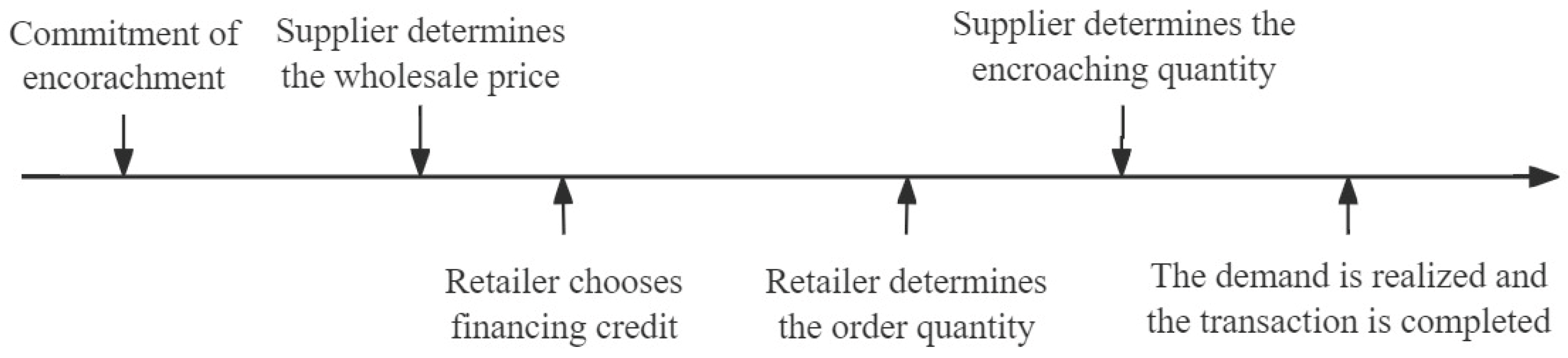
3.1. Model Assumptions

We consider a decentralized supply chain consisting of a supplier (denoted by $s$) and a retailer (denoted by $r$) whose initial capital is $Z\left(Z\ge 0\right)$. The supplier produces and sells products to the retailer at the wholesale price, denoted as w, and then the retailer resells the products to consumers. In addition to the traditional retail channel, the supplier may establish his own direct sales channel with a fixed cost $F$ for selling the product to customers, which could lead to encroachment. We normalize both the supplier’s production cost and the retailer’s selling cost to zero. We adopt a linear downward-sloping inverse demand function $p_i=A_k-q_i-b{q}_{-i}(k=l,h;i=s,r)$, where $p_i$, $q_i$, $b$ and $q_{-i}$ represent the retail price, sales in one channel, channel substitution rate, and sales in the other channel, respectively, and the notation ‘$-i$’ represents the opposite value. The intercept of the demand function, $A_k$, represents the random market potential. We assume that $A_k$ follows a two-point distribution, where $k=l$ represents the state of low market demand and $k=h$ represents the state of high market demand. The linear inverse demand function is widely used in economics, marketing, and operations management studies [31,47,48]. Following prior studies [5,45,49], we assume that two states of demand occur with equal probability, as follows:

$$A_k=\left\{\begin{array}{c}{A}_h=1+a,\hspace{1em}\hspace{1em}\mathrm{with} \mathrm{probability} \frac{1}{2}\\ A_l=1-a,\hspace{1em}\hspace{1em}\mathrm{with} \mathrm{probability} \frac{1}{2}\end{array}\right.$$

(1)

where $a \mathsf{ϵ}[\mathrm{0,1})$ is the measure of demand volatility. Therefore, the demand expectation is $E\left(A_k\right)=\frac{1+a}{2}+\frac{1-a}{2}=1$. When the supplier encroaches on the end market, with a high market demand ($k=h$), the inverse demand functions for the retailer and the supplier are $p_r=A_h-q_r-b{q}_s$ and $p_s=A_h-q_s-b{q}_r$, respectively; with low market demand ($k=l$), the inverse demand functions for the retailer and the supplier are $p_r=A_l-q_r-b{q}_s$ and $p_s=A_l-q_s-b{q}_r$, respectively.

The retailer’s initial capital $Z$ is exogenously and publicly known. The retailer may be capital-sufficient or capital-constrained, depending on the wholesale price and the order quantity. If the retailer is capital-constrained, both bank credit and trade credit are available. We use the tie-breaking rule that the retailer chooses trade credit if there is no difference for the retailer to borrow from the bank and the supplier because the retailer wants to strengthen the relationship with the supplier.

The sequence of events and decisions is illustrated in Figure 1. First, the supplier makes a commitment ex-ante on whether to enter the retail market. Once the encroachment decision is established, it is binding and irreversible. This does not mean the supplier must sell products only through the direct sales channel if it is profitable. The ex-ante consideration of supplier encroachment is frequently used in the previous literature [14,15] because establishing a physical or online store requires investment. Second, the supplier offers a wholesale price contract to the retailer, building upon the encroachment behavior. Third, the retailer decides on the financing strategy, whether to use bank credit or trade credit. Then, the retailer decides the order quantity for the traditional channel. Then, the supplier determines the quantity in the direct sales channel if the supplier decides to encroach. Finally, the demand is realized and the products are sold, and then the supply chain partners collect their revenues.

Both the supplier and the retailer are assumed to be risk-neutral and aim to optimize their expected profits. Backward induction is applied to ensure the subgame perfection due to the game interactions between the supplier and the retailer. For ease of exposition, we use superscripts N and E to indicate the state of non-encroachment and encroachment and use superscripts N and C to indicate a retailer’s situation without and with external financing. Thus, NN denotes the scenario where the retailer has no financing options with non-encroachment, and NE denotes the scenario where encroachment occurs without external financing. When the retailer considers the financing options, T and B indicate trade credit and bank credit, respectively. Then, BN, BE, TN, and TE represent bank credit without encroachment, bank credit with encroachment, trade credit without encroachment, and trade credit with encroachment, respectively. All parameters involved are summarized in

Table 2. Notation and their explanation.

Notation	Explanation
$s$	Supplier
$r$	Retailer
$Z$	Retailer’s initial working capital
$A_k$	Market state, $k=l, h.$ $A_l$ denotes low market demand, $A_h$ denotes high market demand
$p_i$	$i$’s retail price, $i=r,s$
$q_i$	$i$’s sales or order quantity, $i=r,s$
$b$	Channel substitution rate
$a$	$a \mathsf{ϵ}[\mathrm{0,1})$ is the measure of demand volatility
$F$	Supplier’s fixed costs in establishing a direct sales channel
$w$	Wholesale price
${\pi }_i^{y,m}$	$i$’s profit with $y$ financing unde $m$ strategy, $y=N,B,T,$ where $N$ donates without financing, $B$ donates bank credit financing, $T$ donates trade credit financing; $m=N,E,$ where $N$ donates non-encroachment, $E$ donates encroachment

.

3.2. Benchmark Analysis: The Retailer without Financing Options

In this subsection, we investigate the supplier’s encroachment decision when the retailer has no external financing options.

In Case NN, the supplier does not encroach, and the retailer does not consider external financing. The players’ maximization problems are as follows:

$${\pi }_s^{NN}=w^{NN}{q}_r^{NN}$$

(2)

$$\genfrac{}{}{0pt}{}{{E[\pi }_r^{NN}]=E[\left(A_k-q_r^{NN}-w^{NN}\right)q_r^{NN}]}{s.t.w^{NN}{q}_r^{NN}\le Z,{ q}_r^{NN}\ge 0}$$

(3)

In Case $NE$, the supplier encroaches on the retail market and the retailer does not consider external financing. The players’ maximization problems are as follows:

$$E[{\pi }_s^{NE}]=E[\left(A_k-q_s^{NE}-{bq}_r^{NE}\right)q_r^{NE}+w^{NE}{q}_r^{NE}-F]$$

(4)

$$\genfrac{}{}{0pt}{}{{E[\pi }_r^{NE}]=E\left[\left(A_k-q_r^{NE}-b{q}_s^{NE}-w^{NE}\right)q_r^{NE}\right]}{s.t.w^{NE}{q}_r^{NE}\le Z,q_r^{NE}\ge 0}, k=h,l$$

(5)

Through solving the supplier’s and the retailer’s maximization problems, we derived the optimal results under Case NN and Case NE, which are shown in

Table 3. The optimal results under Case NN and Case NE.

	Case NN		Case NE
	$\mathit{Z}\ge \frac{1}{8}$	$\mathit{Z}<\frac{1}{8}$	$\mathit{Z}\ge {\overline{\mathit{Z}}}_1$	$\mathit{Z}<{\overline{\mathit{Z}}}_1$
$w$	$\frac{1}{2}$	$\frac{1-\sqrt{1-8Z}}{2}$	$\frac{b^3-{6b}^2+8}{2(8-5b^2)}$	$\frac{2-b+\sqrt{{(2-b^2)}^2-16Z(2-b^2)}}{4}$
$q_r$	$\frac{1}{4}$	$\frac{1+\sqrt{1-8Z}}{4}$	$\frac{2(1-b)}{8-5b^2}$	$\frac{2-b-\sqrt{{(2-b^2)}^2-16Z(2-b^2)}}{4(2-b^2)}$
$q_s$	$-$	$-$	$\frac{-{3b}^2-2b+8}{2(8-5b^2)}$	$\frac{-{3b}^2-2b+8+b\sqrt{{(2-b^2)}^2-16Z(2-b^2)}}{8(2-b^2)}$
$E[{\pi }_r]$	$\frac{1}{16}$	$\frac{{\left(1+\sqrt{1-8Z}\right)}^2}{16}$	$\frac{2{\left(1-b\right)}^2(2-b^2)}{{(8-5b^2)}^2}$	$\frac{{\left(2-b-\sqrt{{(2-b)}^2-16Z(2-b^2)}\right)}^2}{32(2-b^2)}$
$E[{\pi }_s]$	$\frac{1}{8}$	$Z$	$\frac{-b^2-8b+12}{4(8-5b^2)}-F$	$\frac{{\left(8-3b^2-2b+b\sqrt{{(2-b^2)}^2-16Z(2-b^2)}\right)}^2}{64{(-2+b^2)}^2}+Z-F$

.

Table 3 indicates that initial capital $Z$ affects the optimal results. In Case NN, when $Z\ge \frac{1}{8}$, the retailer has adequate capital, resulting in the equilibrium solutions that represents the optimal outcomes without capital constraints. When $Z<\frac{1}{8}$, the retailer is deemed to be capital-constrained and will place orders using all available initial capital. Similarly, in Case NE, when $Z\ge {\overline{Z}}_1$, the retailer is capital-sufficient, and the equilibrium solutions represent the optimal results without capital constraints. When $Z<{\overline{Z}}_1$, the retailer is capital-constrained. Due to the supplier’s decision to encroach, both channels are competing for consumers.

We use numerical examples to better show the results. In our numerical examples, we set $F=0.001$ to ensure it falls within the feasible region while still enabling positive expected profits for the supplier across different cases. The numerical results under Case NN and Case NE are presented in

Table 4. Numerical results under Case NN and Case NE.

$\mathit{b}$	$\mathit{Z}$	${\mathit{w}}^{\mathit{N}\mathit{N}}$	${\mathit{q}}_{\mathit{r}}^{\mathit{N}\mathit{N}}$	${\mathit{E}\mathbf{[}\mathit{\pi }}_{\mathit{r}}^{\mathit{N}\mathit{N}}\mathbf{]}$	$\mathit{E}\mathbf{[}{\mathit{\pi }}_{\mathit{s}}^{\mathit{N}\mathit{N}}\mathbf{]}$	${\mathit{w}}^{\mathit{N}\mathit{E}}$	${\mathit{q}}_{\mathit{r}}^{\mathit{N}\mathit{E}}$	${\mathit{q}}_{\mathit{s}}^{\mathit{N}\mathit{E}}$	${\mathit{E}\mathbf{[}\mathit{\pi }}_{\mathit{r}}^{\mathit{N}\mathit{E}}\mathbf{]}$	${\mathit{E}\mathbf{[}\mathit{\pi }}_{\mathit{s}}^{\mathit{N}\mathit{N}}\mathbf{]}$
0.1	0.15	$\frac{1}{2}$	$\frac{1}{4}$	$\frac{1}{16}$	$\frac{1}{8}$	0.499	0.226	$0.489$	0.051	$0.342$
0.2	0.25	$\frac{1}{2}$	$\frac{1}{4}$	$\frac{1}{16}$	$\frac{1}{8}$	0.498	0.205	0.479	0.041	$0.330$
0.3	0.35	$\frac{1}{2}$	$\frac{1}{4}$	$\frac{1}{16}$	$\frac{1}{8}$	0.496	0.185	0.472	$0.033$	$0.311$
0.4	0.45	$\frac{1}{2}$	$\frac{1}{4}$	$\frac{1}{16}$	$\frac{1}{8}$	0.493	0.166	0.466	$0.026$	$0.298$

.

We obtain the supplier’s encroachment decision by comparing the supplier’s expected profits in two scenarios, as shown in Proposition 1.

Proposition 1.

When the retailer lacks external financing, the supplier’s optimal encroachment decision is as follows:

(1) 

when the entry cost $F$ is high, i.e., $F\ge max\left\{F*\left(Z\right),\frac{b^2+2b-4}{16{(2-b^2)}^2}\right\}$, the supplier’s best choice is non-encroachment;

(2) 

when the entry cost $F$ is medium, i.e.,  $\frac{{3b}^2-16b+16}{8(8-5b^2)}<F\le max\left\{F*\left(Z\right),\frac{b^2+2b-4}{16{(2-b^2)}^2}\right\}$, if $F\le \overline{F}\left(Z\right)$, the supplier encroaches; if $F>\overline{F}\left(Z\right)$, the supplier never encroach;

(3) 

when the entry cost $F$ is low, i.e., $F\le \frac{{3b}^2-16b+16}{8(8-5b^2)}$, the supplier’s best choice is encroachment.

Proposition 1 illustrates the supplier’s encroachment decision when external financing is unavailable. The encroachment decision will have two obvious impacts: on one hand, the supplier can increase sales and revenue through encroachment; on the other hand, the supplier needs to incur certain costs when establishing a direct sales channel. Therefore, the supplier’s encroachment decision is based on the tradeoff between his increasing revenue and the entry cost. Furthermore, the threshold of the entry cost is jointly determined by the channel substitution rate $b$ and the retailer’s initial capital $Z$.

Through the comparison of the equilibrium solutions in the cases with and without supplier encroachment, Proposition 2 summarizes the effects of supplier encroachment on the wholesale price, retailer’s order quantity, and retailer’s expected profit.

Proposition 2.

Without external financing choices,

(1) 

$w^{NE}\le w^{NN}$;

(2) 

when $Z<Z_2$, $q_r^{NE}\le q_r^{NN}$; when $Z_2\le Z<\frac{2(4-9b^2+5b^3)}{{(8-5b^2)}^2}$, $q_r^{NE}>q_r^{NN}$; when $\frac{2(4-9b^2+5b^3)}{{(8-5b^2)}^2}\le Z$, $q_r^{NE}\le q_r^{NN}$;

(3) 

when $Z<Z_3$, ${E[\pi }_r^{NN}]\le {E[\pi }_r^{NE}]$; when $Z_3\le Z$, ${E[\pi }_r^{NN}]>{E[\pi }_r^{NE}]$.

When the supplier encroaches, the supplier lowers the wholesale price to meet the retailer’s demand. When the initial capital $Z$ is moderate, the retailer’s order quantity under supplier encroachment is high. When the retailer’s initial capital $Z$ is either low or high, the order quantity under supplier encroachment is small. The reason is that the retailer’s order quantity decreases with either less initial capital or intense competition. Under the combined influence of the wholesale price and order quantity, when the initial capital $Z$ is low, supplier encroachment benefits the retailer; otherwise, it is detrimental to the retailer’s profit.

4. Equilibrium When Considering Retailer’s Financing Options

In this section, we present the equilibria for each case based on the financing strategy and the supplier’s encroachment decision. Then, we investigate the impacts of supplier encroachment and financing strategies.

4.1. Equilibria under Trade Credit

We first consider the cases where the retailer adopts trade credit financing, i.e., Case TN and Case TE. Under trade credit financing, the retailer borrows credit from the supplier when she is capital-constrained.

In Case TN, the sequence of events is as follows. The supplier determines the wholesale price based on the retailer’s initial capital. And the retailer determines the order quantity accordingly. Then, the demand is realized. If the retail’s revenue exceeds the wholesale cost, the supplier receives a repayment of $w^{TN}{q}_r^{TN}$. If the retail revenue does not exceed the wholesale cost, the supplier receives a repayment of the total retail revenue plus the retailer’s initial capital (either partially or in full). The expected profit functions for the supplier and the retailer are as follows:

$$E{[\pi }_s^{TN}]=\frac{1}{2}{w}^{TN}{q}_r^{TN}+\frac{1}{2}min\left\{w^{TN}{q}_r^{TN},\left(1-a-q_r^{TN}\right)q_r^{TN}+Z\right\}$$

(6)

$$E{[\pi }_r^{TN}]=\frac{1}{2}\left(1+a-q_r^{TN}-w^{TN}\right)q_r^{TN}+\frac{1}{2}\left\{\mathrm{m}\mathrm{a}\mathrm{x}\left[\left(1-a-q_r^{TN}\right)q_r^{TN}-\left(w^{TN}{q}_r^{TN}-Z\right),0\right]-Z\right\}$$

(7)

The first part of each function represents the supplier’s or retailer’s profit when the retailer does not declare bankruptcy due to high demand, while the second part represents the supplier’s or retailer’s profit when the retailer declares bankruptcy due to low demand.

In Case TE, the sequence of events is as follows. The supplier commits to entering the retail market and sets the wholesale price, considering that the retailer will postpone her payment. The retailer then determines the order quantity accordingly. After that, the supplier determines the encroaching quantity. In the end, the demand is realized, and the retailer pays the delayed payment to the supplier (the full repayment or partial repayment if the retailer declares bankruptcy), completing the transaction.

The retailer’s expected profit function is as follows:

$$E{[\pi }_r^{TE}]=\left\{\begin{array}{c}\frac{1}{2}{q}_r^{TE}\left(1+a-q_r^{TE}-b{q}_s^{TE}-w^{TE}\right)+\\ +\frac{1}{2}\left\{max\left[q_r^{TE}\left(1-a-q_r^{TE}-b{q}_s^{TE}\right)-\left(w^{TE}{q}_r^{TE}-Z\right),0\right]-Z\right\}\end{array}\right\}$$

(8)

The first part of the function represents the profit if the retailer does not go bankrupt due to high demand, while the second part represents the profit when the retailer goes bankrupt due to low demand.

The supplier’s expected profit function is as follows:

$$E{[\pi }_s^{TE}]=\left\{\begin{array}{c}\frac{1}{2}{w}^{TE}{q}_r^{TE}+\frac{1}{2}min\left\{w^{TE}{q}_r^{TE},\left(1-a-q_r^{TE}-b{q}_s^{TE}\right)q_r^{TE}+Z\right\}\\ +\{\left(1-{bq}_r^{TE}-q_s^{TE}\right)q_s^{TE}-F\}\end{array}\right\}$$

(9)

The first part of the function represents the profit if the retailer does not go bankrupt due to high demand, while the second part represents the profit if the retailer goes bankrupt due to low demand. The third part represents the supplier’s expected profit from encroachment.

Through solving the supplier and the retailer’s expected profit functions, we derived the optimal results under Case TN and Case TE, which are presented in

Table 5. The optimal results are under Case TN and Case TE.

	Case TN		Case TE
	$\mathit{a}\le {\overline{\mathit{a}}}_1$	$\mathit{a}>{\overline{\mathit{a}}}_1$	$\mathit{a}\le {\overline{\mathit{a}}}_2$	$\mathit{a}>{\overline{\mathit{a}}}_2$
$w$	$\frac{1}{2}$	$\frac{3a+1}{3}$	$\frac{8-6b^2+b^3}{2(8-5b^2)}$	$a+\frac{6+b}{14}-\frac{16(1-b)}{21(8-7b^2)}$
$q_r$	$\frac{1}{4}$	$\frac{1}{3}$	$\frac{2(1-b)}{8-5b^2}$	$\frac{8(1-b)}{3(8-7b^2)}$
$q_s$	$-$	$-$	$\frac{8-2b-3b^2}{2(8-5b^2)}$	$\frac{1}{2}-\frac{2b(1-b)}{(8-7b^2)}$
$E[{\pi }_r]$	$\frac{1}{16}$	$\frac{1}{18}-\frac{Z}{2}$	$\frac{2(2-b^2){(1-b^2)}^2}{{(8-5b^2)}^2}$	$\frac{8{(1-b)}^2(4-3b^2)}{9{(8-7b^2)}^2}-\frac{Z}{2}$
$E[{\pi }_s]$	$\frac{1}{8}$	$\frac{1+3Z}{9}$	$\frac{-b^2-8b+12}{4(8-5b^2)}-F$	$\frac{-5b^2-32b+40}{12{(8-7b^2)}^2}+\frac{Z}{2}-F$

.

Table 5 indicates that the demand uncertainty $a$ affects the optimal results. In Case TN, when the demand uncertainty is low, i.e., $a<{\overline{a}}_1$, there is no risk of bankruptcy for the retailer. Therefore, the retailer’s order quantity under trade credit financing is the same as that under bank credit financing. When the demand uncertainty is high, i.e., ${\overline{a}}_1\le a$, the supplier will be more aggressive in wholesale pricing due to the retailer’s risk of bankruptcy. The retailer will be more aggressive in determining the order quantity. As a result, the retailer’s order quantity under trade credit differs from that under bank credit financing. Under trade credit financing, the supplier assumes the retailer’s bankruptcy risk, which is influenced by demand fluctuation. The wholesale price is influenced by demand uncertainty, while the retailer’s order quantity remains unaffected by demand uncertainty.

In Case TE, when market demand uncertainty $a$ is low, the retailer is less likely to go bankrupt. Both the supplier and the retailer behave the same way when the retailer has abundant initial capital in the benchmark model. When demand uncertainty $a$ is high, it increases the likelihood of the retailer going bankrupt. The supplier adjusts the wholesale price based on demand uncertainty to mitigate the risk of bankruptcy. The retailer behaves aggressively to order. The supplier, however, acts cautiously when deciding on the order quantity due to the retailer’s aggressive behavior, which escalates competition in the downstream retail market.

The numerical results under Case TN and Case TE are presented in

Table 6. Numerical results under Case TN and Case TE.

$\mathit{b}$	$\mathit{Z}$	$\mathit{a}$	${\mathit{w}}^{\mathit{T}\mathit{N}}$	${\mathit{q}}_{\mathit{r}}^{\mathit{T}\mathit{N}}$	${\mathit{E}\mathbf{[}\mathit{\pi }}_{\mathit{r}}^{\mathit{T}\mathit{N}}\mathbf{]}$	$\mathit{E}\mathbf{[}{\mathit{\pi }}_{\mathit{s}}^{\mathit{T}\mathit{N}}\mathbf{]}$	${\mathit{w}}^{\mathit{T}\mathit{E}}$	${\mathit{q}}_{\mathit{r}}^{\mathit{T}\mathit{E}}$	${\mathit{q}}_{\mathit{s}}^{\mathit{T}\mathit{E}}$	${\mathit{E}\mathbf{[}\mathit{\pi }}_{\mathit{r}}^{\mathit{T}\mathit{E}}\mathbf{]}$	${\mathit{E}\mathbf{[}\mathit{\pi }}_{\mathit{s}}^{\mathit{T}\mathit{E}}\mathbf{]}$
0.1	0.1	0.1	$0.433$	$\frac{1}{3}$	$0.006$	$0.144$	0.499	0.226	$0.489$	0.062	$0.351$
0.2	0.3	0.4	$\frac{1}{2}$	$\frac{1}{4}$	$\frac{1}{16}$	$\frac{1}{8}$	0.498	0.205	0.479	0.059	$0.331$
0.3	0.5	0.7	$\frac{1}{2}$	$\frac{1}{4}$	$\frac{1}{16}$	$\frac{1}{8}$	0.496	0.185	0.472	$0.055$	$0.314$
0.4	0.7	1	$\frac{1}{2}$	$\frac{1}{4}$	$\frac{1}{16}$	$\frac{1}{8}$	0.493	0.167	0.467	$0.050$	$0.299$

.

4.2. Equilibria under Bank Credit

Now we study the cases where the retailer adopts bank credit financing, i.e., Cases BN and BE. Under bank credit financing, the retailer borrows from the bank when they are capital-constrained.

In Case BN, the retailer borrows from the bank when she is capital-constrained and the supplier does not encroach. The bank lending market is assumed to be perfectly competitive, and the bank earns zero expected profit. This is equivalent to the retailer being capital-sufficient, as there are no lending costs associated with bank credit financing. Therefore, since the bank does not generate any profit from lending to the retailer, the bank’s lending cost of the loan is equal to the expected return from the loan. The zero-profit condition is $w^{BN}{q}_r^{BN}-Z=E\left\{min\left[\left(w^{BN}{q}_r^{BN}-Z\right)\left(1+t^{BN}\right),\left(A_k-q_r^{BN}\right)q_r^{BN}-Z\right]\right\},k=h,l$. The supplier then determines the wholesale price, contingent upon the retailer being offered bank credit financing. The retailer determines the order quantity based on the wholesale price and borrows bank loans to pay for the procured products. Once the demand is realized, the transaction is completed. The supplier’s optimal wholesale price problem is to maximize:

$$E{[\pi }_s^{BN}]=w^{BN}{q}_r^{BN}$$

(10)

The retailer’s problem is to determine the order quantity for maximizing his expected profit, $E{[\pi }_r^{BN}]=max\left\{\left(A_k-q_r^{BN}\right)q_r^{BN}-\left(w^{BN}{q}_r^{BN}-Z\right)\left(1+t^{BN}\right),0\right\}$. When the retailer orders $q_r^{BN}$, he will anticipate the corresponding interest rate $t^{BN}$ as provided in the zero-profit condition of the bank. When the products are sold, the retailer collects the revenue of $\left(A_k-q_r^{BN}\right)q_r^{BN}$, $k=h/l$. Then, she uses this to repay her debt (including the loan’s principal and interest and her initial capital). Similar to the Lemma 1 of Jing et al. [12], the retailer’s optimization problem is equivalent to the benchmark model when the retailer is capital-sufficient as follows:

$$E{[\pi }_r^{BN}]=E[\left(A_k-q_r^{BN}-w^{BN}\right)q_r^{BN}]$$

(11)

In Case BE, we investigate the scenario where the retailer has access to bank credit financing, and the supplier enters the retail market. The sequence of events is as follows. The supplier commits to entering the retail market and sets the wholesale price, considering that the retailer is offered bank credit financing. The retailer then determines the order quantity based on the wholesale price and borrows money from the bank. The supplier adjusts the quantity accordingly to encroachment. Once the demand is realized, the retailer repays the loan to the bank, either in full or partially if bankruptcy occurs. Finally, the transaction is completed.

Similar to Case BN, the retailer’s issue is comparable to that scenario where she is not capital-constrained. Thus, the supply chain members’ expected profit functions are as follows:

$$E{[\pi }_r^{BE}]=E[\left(A_k-q_r^{BE}-b{q}_s^{BE}-w^{BE}\right)q_r^{BE}],k=h,l;$$

(12)

$$E{[\pi }_s^{BE}]=E[\left(A_k-{bq}_r^{BE}-q_s^{BE}\right)q_s^{BE}+w^{BE}{q}_s^{BE}-F], k=h,l$$

(13)

Through solving the supplier and the retailer’s expected profit functions, we derived the optimal results under Case BN and Case BE, which are shown in

Table 7. The optimal results under Case BN and Case BE.

	Case BN	Case BE
$w$	$\frac{1}{2}$	$\frac{8-6b^2+b^3}{2(8-5b^2)}$
$q_r$	$\frac{1}{4}$	$\frac{2(1-b)}{8-5b^2}$
$q_s$	$-$	$\frac{8-2b-3b^2}{2(8-5b^2)}$
$E[{\pi }_r]$	$\frac{1}{16}$	$\frac{2(2-b^2){(1-b^2)}^2}{{(8-5b^2)}^2}$
$E[{\pi }_s]$	$\frac{1}{8}$	$\frac{-b^2-8b+12}{4(8-5b^2)}-F$

.

Table 7 indicates that when the retailer is financed with bank credit, the bank acts as a risk buffer and provides the necessary funds for the retailer. The retailer has sufficient working capital to place an order with the supplier. Simultaneously, the supplier can obtain more profit through wholesale pricing, no longer bearing the potential risk of retailer bankruptcy.

The numerical results under Case BN and Case BE are presented in

Table 8. Numerical results under Case BN and Case BE.

$\mathit{b}$	${\mathit{w}}^{\mathit{B}\mathit{N}}$	${\mathit{q}}_{\mathit{r}}^{\mathit{B}\mathit{N}}$	${\mathit{E}\mathbf{[}\mathit{\pi }}_{\mathit{r}}^{\mathit{B}\mathit{N}}\mathbf{]}$	$\mathit{E}\mathbf{[}{\mathit{\pi }}_{\mathit{s}}^{\mathit{B}\mathit{N}}\mathbf{]}$	${\mathit{w}}^{\mathit{B}\mathit{E}}$	${\mathit{q}}_{\mathit{r}}^{\mathit{B}\mathit{E}}$	${\mathit{q}}_{\mathit{s}}^{\mathit{B}\mathit{E}}$	${\mathit{E}\mathbf{[}\mathit{\pi }}_{\mathit{r}}^{\mathit{B}\mathit{E}}\mathbf{]}$	${\mathit{E}\mathbf{[}\mathit{\pi }}_{\mathit{s}}^{\mathit{B}\mathit{E}}\mathbf{]}$
0.2	$\frac{1}{2}$	$\frac{1}{4}$	$\frac{1}{16}$	$\frac{1}{8}$	0.498	0.205	$0.479$	0.059	$0.331$
0.4	$\frac{1}{2}$	$\frac{1}{4}$	$\frac{1}{16}$	$\frac{1}{8}$	0.493	0.167	0.467	0.050	$0.299$
0.6	$\frac{1}{2}$	$\frac{1}{4}$	$\frac{1}{16}$	$\frac{1}{8}$	0.488	0.129	0.461	$0.035$	$0.275$
0.8	$\frac{1}{2}$	$\frac{1}{4}$	$\frac{1}{16}$	$\frac{1}{8}$	0.486	0.083	0.467	$0.015$	$0.257$

.

5. Impacts of Financing Strategies and Encroachment

In this section, we investigate how the financing and encroachment strategies affect the supply chain partners’ profits.

5.1. The Effects of Financing Strategies

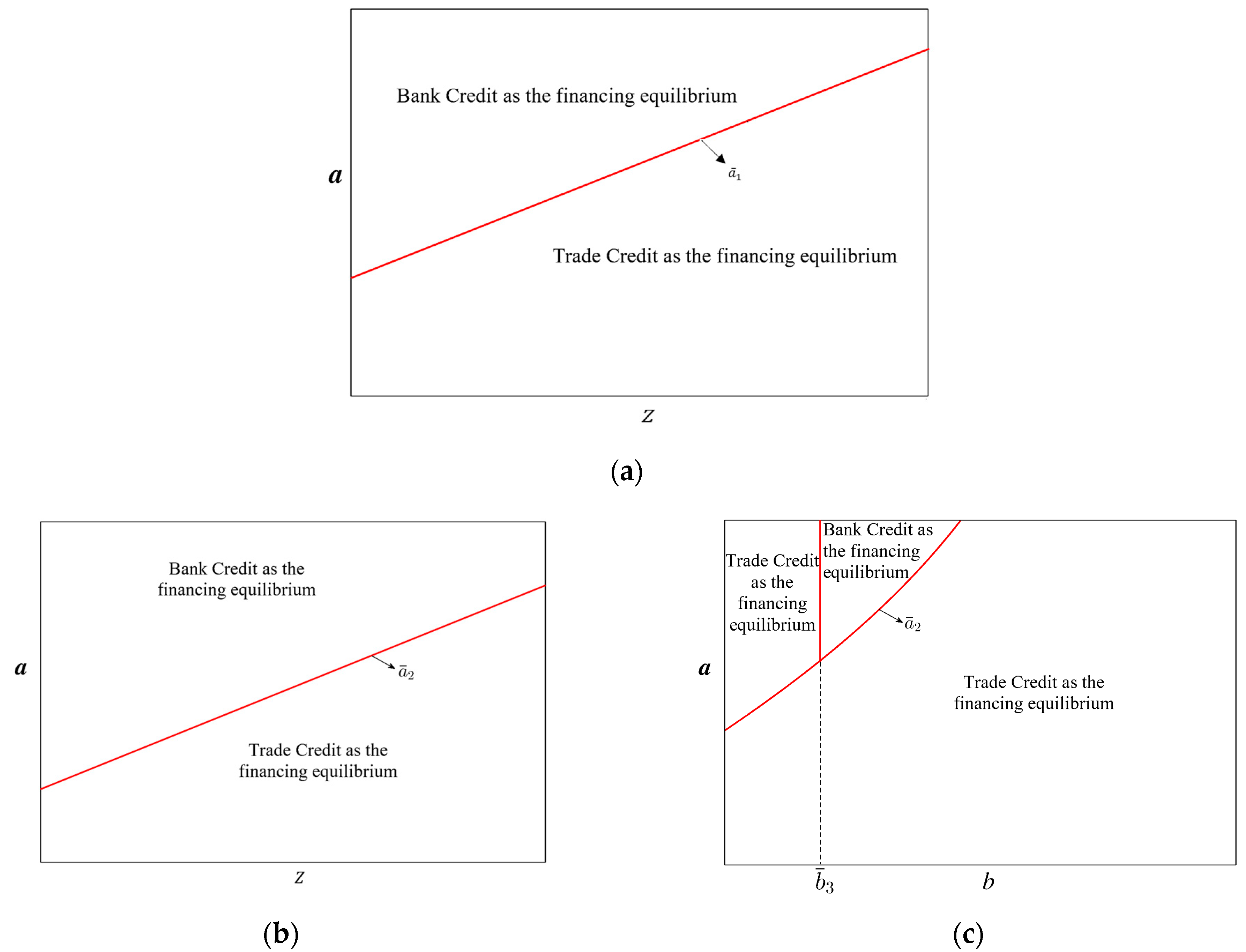
In this subsection, we compare the retailer’s financing choices between bank credit and trade credit financing under different situations.

Through the comparison of the expected profits under trade credit and bank credit financing, we can determine the impacts of financing strategies on the supply chain members in Proposition 3.

Proposition 3.

Regardless of the supplier’s decision to encroach, the supplier always benefits from trade credit. The impacts of this financing strategy on the retailer are as follows:

(1) 

Without encroachment, when $a<{\overline{a}}_1$, the retailer always chooses trade credit; when ${\overline{a}}_1\le a<1$, the retailer chooses bank credit;

(2) 

With encroachment, the retailer’s financing decision is jointly determined by the demand volatility rate $a$ and the channel substitution rate $b$. When $a<{\overline{a}}_2$, the retailer always chooses trade credit financing. When ${\overline{a}}_2\le a<1$, the retailer chooses trade credit financing if b is low and otherwise the retailer chooses bank credit financing.

Proposition 3 indicates that the financing strategy has different effects on the supplier and the retailer. The supplier always benefits from trade credit financing, regardless of his decision to encroach. However, the retailer chooses her financing strategy according to the tie-breaking rule. Proposition 3(2) shows that the retailer with a high credit risk (i.e., higher a) tends to choose bank credit rather than trade credit, as shown in Figure 2a. When $a<{\overline{a}}_1$, the demand volatility rate is low, and the retailer has no bankruptcy risk. Therefore, there is no difference between trade credit and bank credit for the retailer. According to the tie-breaking rule, the retailer chooses trade credit. When ${\overline{a}}_1<a<1$, the demand volatility rate is high, and the retailer faces the risk of bankruptcy. Hence, the supplier’s expected profit consists of two parts: the full payment if the retailer does not declare bankruptcy and partial payment if the retailer does declare bankruptcy. Therefore, the supplier will be more aggressive in pricing, thereby increasing profits. The retailer’s profit in the case of bank credit is always higher (or equal). This is because the bank credit financing market is completely competitive. Banks can not only provide funds for the retailer but also bear the costs of the retailer’s bankruptcy risk. When the retailer chooses trade credit, although the supplier bears a part of the bankruptcy risk, the retailer’s profit will be squeezed due to the supplier’s aggressive pricing behavior. Figure 2a shows the retailer’s optimal financing choice without supplier encroachment.

Figure 2b,c depict the retailer’s equilibrium financing choices with supplier encroachment in the retail market. With supplier encroachment, the retailer’s credit financing decision is jointly determined by the demand volatility rate and the channel substitution rate. When $a<{\overline{a}}_2$, the market demand is relatively stable, and the retailer will not need to declare bankruptcy. The retailer chooses trade credit financing based on the tie-breaking rule. When ${\overline{a}}_2<a<1$, the market demand is unstable, and the retailer is more likely to declare bankruptcy. The supplier’s decision to encroach could increase the competition in the downstream retail market, thereby intensifying this risk. When the realized market demand is high, the supplier increases the wholesale price to maximize profit, which is used as a strategy for mitigating the risk of the retailer’s bankruptcy. The retailer behaves aggressively when ordering products by choosing trade credit financing. Therefore, when the channel substitution $b$ is high, the retailer opts for bank credit financing because of intense downstream competition, the supplier’s aggressive wholesale price determination, and the retailer’s crucial order quantity determination. When the channel substitution rate $b$ is low, downstream competition is not intense, and the supplier is conservative in determining the quantity of encroachment, the retailer chooses trade credit financing.

5.2. The Effects of Supplier Encroachment

In this section, we analyze the effects of the supplier’s encroachment decisions on optimal decisions and the economic welfare of supply chain members.

Through the comparison of the wholesale price and order quantity in the case of supplier encroachment and non-encroachment when the retailer has external financing, we can obtain the impacts of encroachment on operational decisions, as given in Proposition 4.

Proposition 4.

When the retailer has access to both bank credit and trade credit financing:

(1) 

the wholesale price under supplier encroachment is smaller than that under no encroachment;

(2) 

when $Z\le {\overline{Z}}_2$, ${\overline{a}}_2\le a\le {\overline{a}}_1$, $0<b<\frac{1}{3}(3-\sqrt{3})$, the retailer’s order quantity under supplier encroachment is smaller than that under no encroachment; otherwise, the retailer’s order quantity under supplier encroachment is higher than that under no encroachment.

Proposition 4 demonstrates that the wholesale price is lower when there is supplier encroachment compared to the case without encroachment. The supplier reduces the wholesale price to stimulate retailer demand when entering the retail market. In addition, the influence of supplier encroachment on the order quantity is not solely dependent on the retailer’s initial capital. When the level of demand uncertainty is low, the likelihood of the retailer declaring bankruptcy decreases. Despite the reduction in wholesale price, the retailer chooses to decrease her order quantity because of the heightened competition in the downstream retail market resulting from the supplier’s encroachment. When facing high demand uncertainty, the retailer is more prone to declaring bankruptcy. The determination of the wholesale price by the supplier remains consistent regardless of the presence or absence of supplier encroachment and is contingent upon the degree of demand uncertainty. The retailer decreases her order quantity in response to the supplier’s encroachment because it results in increased downstream competition. When the initial capital of the retailer is limited and there is a moderate level of demand uncertainty, the likelihood of the retailer declaring bankruptcy increases because of supplier encroachment. If there is no encroachment, then the retailer is less likely to declare bankruptcy. The retailer displays assertive behavior when placing orders for products, even in the face of supplier encroachment. When the rate of channel substitution is low, the level of downstream competition remains relatively low because the limited impact of substitution mitigates the intense competition. Then, the order quantity increases significantly when the supplier engages in encroachment, as opposed to when there is no encroachment.

Through the comparison of the supplier’s expected profits under non-encroachment and encroachment, we can determine the impact of different financing strategies on the supplier’s incentive to encroach. The results are presented in the following proposition.

Proposition 5.

(1) When the entry cost $F$ is high, i.e., $F>{\overline{F}}_1$, the supplier experiences economic damage as a result of encroachment;

(2) when ${\overline{F}}_3<F\le {\overline{F}}_1$, if $Z>{\overline{Z}}_2$, the supplier experiences economic damage as a result of encroachment; if $0\le Z\le {\overline{Z}}_2$, the supplier’s encroachment decision varies from encroachment to no encroachment, and then to encroachment with the increase in$a$;

(3) when ${\overline{F}}_4<F\le {\overline{F}}_3$, the supplier benefits from encroachment when $a$ is high and otherwise does not encroach;

(4) when ${\overline{F}}_2<F\le {\overline{F}}_4$, if $Z>{\overline{Z}}_2$, the supplier’s encroachment decision varies from encroachment to non-encroachment, and then to encroachment with the increase in $a$; if $0\le Z\le {\overline{Z}}_2$, the supplier always benefits from encroachment;

(5) when the entry cost $F$ is low, i.e., $0<F\le {\overline{F}}_2$, the supplier always benefits from encroachment.

Proposition 5 summarizes the supplier’s decision to encroach. When the entry cost is extremely high, i.e., $F>{\overline{F}}_1$, the supplier will refrain from encroaching due to the high expenses associated with establishing a direct sales channel. When the entry cost is high, i.e., ${\overline{F}}_3<F\le {\overline{F}}_1$, the supplier’s encroachment decision is influenced by the retailer’s initial capital and demand uncertainty. If the amount of the initial capital is large, the supplier will not encroach. If the amount of the retailer’s initial capital is small, the supplier will not encroach in cases of high- or low-demand volatility rate but will encroach when there is a medium-demand volatility rate. The reasons are as follows. On one hand, having abundant initial capital reduces the risk of a retailer declaring bankruptcy. On the other hand, if the supplier encroaches on the downstream retail market, it intensifies competition and increases the risk of a retailer declaring bankruptcy. This, in turn, discourages the supplier from encroaching. The lack of initial capital can easily lead to bankruptcy for the retailer, while moderate demand volatility encourages the supplier to take over. When there is either high- or low-demand uncertainty, the supplier’s wholesale price tends to be either moderate or aggressive, regardless of whether there is supplier encroachment. As a result, the limited benefits brought by encroachment cannot offset the entry cost, and the supplier will not encroach. When there is medium-demand uncertainty, making an aggressive wholesale price decision with encroachment brings greater benefits to the supplier. Figure 3a illustrates the supplier’s encroachment decision if $0\le Z\le {\overline{Z}}_2$. When the entry cost is moderate, i.e., ${\overline{F}}_4<F\le {\overline{F}}_3$, the supplier encroaches if the demand uncertainty is high; otherwise, the supplier does not encroach. The reason is that with high-demand uncertainty, the retailer is more likely to declare bankruptcy, resulting in the supplier’s aggressive wholesale pricing. The wholesale price is the same for both situations of encroachment and non-encroachment. Furthermore, in order to avoid intense competition and supplier encroachment in the downstream retail market, the retailer reduces the order quantity, which also decreases the risk of bankruptcy. Thus, the benefits of supplier encroachment include increased sales revenue and a reduced risk of bankruptcy for the retailer, which outweighs the costs of entry. When the entry cost is low, that is ${\overline{F}}_2<F\le {\overline{F}}_4$, the supplier’s decision to encroach is determined by the retailer’s initial capital and demand uncertainty. If the retailer has abundant initial capital, the supplier will engage in encroachment with high- or low-demand uncertainty, but will not engage with medium-demand uncertainty. However, if the initial capital is small, the supplier will always encroach. A low entry cost and a small initial capital level facilitate the supplier’s ability to establish his direct sales channel. When the retailer’s initial capital is substantial and demand uncertainty is moderate, the supplier can benefit more from non-encroachment than from encroachment, because of the supplier’s aggressive wholesale pricing behavior. Figure 3b illustrates the supplier’s encroachment decision if $Z>{\overline{Z}}_2$. When the entry cost is extremely low, i.e., $0<F\le {\overline{F}}_2$, the supplier will always benefit from entering the retail market.

Through the comparison of the retailer’s expected profits under non-encroachment and encroachment, Proposition 6 examines the impacts of encroachment on the retailer.

Proposition 6.

(1) When $a<min\{{\overline{a}}_1,{\overline{a}}_2\}$ or $max\{{\overline{a}}_1,{\overline{a}}_2\}\le a<1$, the retailer is worse off with supplier encroachment;

(2) when $min\{{\overline{a}}_1,{\overline{a}}_2\}\le a<max\{{\overline{a}}_1,{\overline{a}}_2\}$, there exists a threshold of ${\overline{Z}}_3$ where the retailer is better off when $Z$ is larger than ${\overline{Z}}_3$and the retailer is worse off otherwise.

Proposition 6 shows that the impact of supplier encroachment on the retailer depends on the demand volatility rate and the initial capital investment. In most cases, supplier encroachment will be harmful to the retailer. This is because the supplier fails to manage the risks of demand volatility in the supply chain by offering trade credit and increasing downstream competition. While previous studies have suggested that retailers could benefit from supplier encroachment, it is important to note that the retailer may only benefit from encroachment if they can choose the type of credit financing.

When the retailer has large initial capital and the demand volatility rate is medium, the likelihood of the retailer declaring bankruptcy decreases due to encroachment; however, the likelihood of bankruptcy without encroachment increases. When the supplier does not encroach, the retailer’s aggressive behavior in ordering products may cause her to lose her initial capital. However, when the supplier encroaches, the retailer orders a smaller quantity of the product, and the wholesale price decreases. Although the retailer’s expected profit from sales under supplier encroachment may be smaller than that under no encroachment, she would not lose her initial capital. Hence, the retailer benefits from supplier encroachment under this condition.

6. Conclusions

Trade and bank credit financing are common business practices in various industries worldwide. Using the Stackelberg game framework, we examined the roles of trade and bank credit financing in a supply chain that included a supplier and a retailer with limited initial capital. We studied the financing equilibria under two scenarios: supplier encroachment and no encroachment. The innovation of this study can be concluded from the following aspects. First, our study offers a distinctive operational perspective that complements existing literature by addressing the intertwined dynamics of supplier encroachment and credit financing while considering the retailer’s initial working capital. Second, we contribute novel insights by calculating the thresholds of a retailer’s initial working capital under different scenarios, distinguishing between situations where the retailer is capital-constrained or capital-sufficient. This analytical approach offers practical guidance for retailers in determining optimal financing strategies. Third, we reveal nuanced patterns in supplier encroachment decisions under varying conditions. Specifically, our findings highlight the binary nature of supplier encroachment decisions, which may transition from encroachment to no encroachment and then back to encroachment in response to changes in demand volatility rates, particularly when entry costs are moderate.

The main findings of this study are summarized as follows.

(1)

When the supplier does not compete in the retail market, the retailer opts for trade credit financing when the demand volatility is low. The threshold is determined by the retailer’s initial capital and the production cost. When the supplier encroaches, the rate of product substitution becomes a crucial factor in determining the retailer’s choice of credit financing. If the demand volatility and product substitution rates are high, the retailer will opt for bank credit financing. Otherwise, they will choose trade credit financing. The supplier always benefits from the choice of trade credit financing when both financing options are available, whether they are utilized or not;

(2)

The supplier’s wholesale price under supplier encroachment is lower than that under no encroachment. The retailer’s order quantity under supplier encroachment is also lower than that under no encroachment, except when the retailer’s initial capital and the product substitution rate are small, and the demand volatility rate is medium;

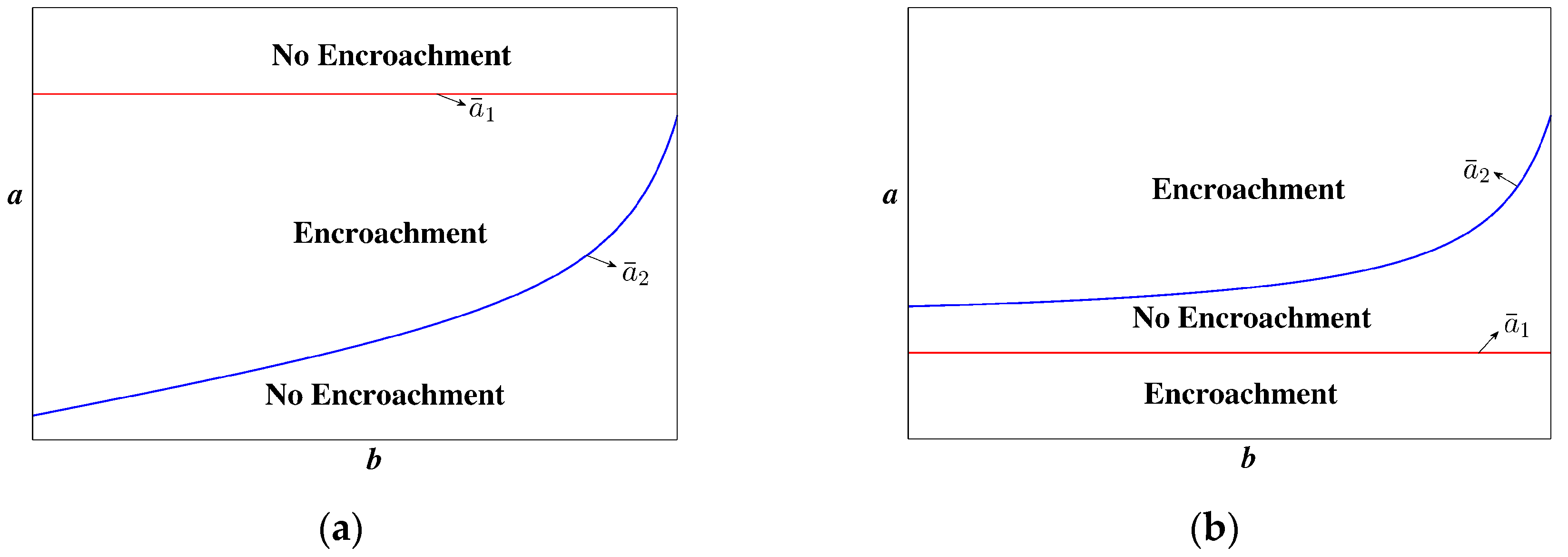
(3)

The supplier’s decision to encroach is primarily determined by the entry cost when the retailer has no access to credit. The supplier encroaches on the retail market when the entry cost is low but otherwise refrains from doing so. When both financing options are available, the supplier’s decision to encroach is jointly determined by the entry cost, the demand volatility rate, and the retailer’s initial working capital. The supplier never enters the market when the entry cost is too high; however, they always enter the market when the entry cost is very low. When the entry cost is moderate, the supplier’s decision on encroachment varies from no encroachment to encroachment, or from no encroachment to encroachment, and then to encroachment again, with the increase in demand volatility, and depending on the retailer’s initial working capital.

Based on our findings in this study, several managerial implications can be derived as follows.

(1)

The retailer should consider the level of demand volatility and the presence of product substitution when making financing decisions. When the supplier does not compete in the retail market, trade credit financing may be preferable under low demand volatility. However, if the supplier encroaches and demand volatility is high, it might be more beneficial to opt for bank credit financing. The retailer should carefully assess these factors when choosing the financing strategy;

(2)

The supplier needs to carefully consider the impact of encroachment on wholesale pricing and order quantity. Under supplier encroachment, the wholesale price tends to decrease, and the retailer may order smaller quantities, particularly when initial capital and product substitution rates are low, and demand volatility is medium. The supplier should evaluate these factors to adjust his pricing and inventory strategy accordingly;

(3)

The supplier should evaluate the entry cost, demand volatility, and the retailer’s working capital when considering entering the retail market. When the retailer has no access to credit, the decision to encroach is primarily influenced by the entry cost; however, if both financing options are available, then the supplier should consider more factors. The supplier should also assess these factors to determine the optimal timing and conditions for entering the retail market.

Future research could expand in the following several directions. Firstly, the current study only considers one downstream retailer. Future research could explore scenarios involving two or multiple competing retailers, examining the impact of competitive relationships on the supplier’s channel selection and the retailer’s financing strategies. Secondly, it is noteworthy that retailers usually keep their financial information private. One future possibility is to explore how retailers strategically disclose their financial information to influence suppliers. Thirdly, while this study assumes that downstream retailers may face financial constraints, it is essential to acknowledge that upstream suppliers may also encounter financial limitations. Thus, it would be worthwhile to study the financing decisions and channel strategies of suppliers under various financial conditions.

References

1. Arya, A.; Mittendorf, B.; Sappington, D.E. The bright side of supplier encroachment. Market.Sci. 2007, 26, 651–659. [Google Scholar] [CrossRef]
2. Guan, H.; Gurnani, H.; Geng, X.; Luo, Y. Strategic inventory and supplier encroachment. Manuf. Serv. Oper. Manag. 2019, 21, 536–555. [Google Scholar] [CrossRef]
3. Emtehani, F.; Nahavandi, N.; Rafiei, F.M. Trade credit financing for supply chain coordination under financial challenges: A multi-leader–follower game approach. Financ. Innov. 2023, 9, 6. [Google Scholar] [CrossRef]
4. Li, Y.; Wu, D.; Dolgui, A. Optimal trade credit coordination policy in dual-channel supply chain with consumer transfer. Int. J. Prod. Res. 2022, 60, 4641–4653. [Google Scholar] [CrossRef]
5. Zhang, L.-H.; Zhang, C.; Yang, J. Impacts of power structure and financing choice on manufacturer’s encroachment in a supply chain. Ann. Oper. Res. 2023, 322, 273–319. [Google Scholar] [CrossRef]
6. An, S.; Li, B.; Song, D.; Chen, X. Green credit financing versus trade credit financing in a supply chain with carbon emission limits. Eur. J. Oper. Res. 2021, 292, 125–142. [Google Scholar] [CrossRef]
7. Yan, N.; He, X.; Liu, Y. Financing the capital-constrained supply chain with loss aversion: Supplier finance vs. supplier investment. Omega 2019, 88, 162–178. [Google Scholar] [CrossRef]
8. Yuan, X.; Bi, G.; Fei, Y.; Liu, L. Supply chain with random yield and financing. Omega 2021, 102, 102334. [Google Scholar] [CrossRef]
9. Deng, S.; Fu, K.; Xu, J.; Zhu, K. The supply chain effects of trade credit under uncertain demands. Omega 2021, 98, 102113. [Google Scholar] [CrossRef]
10. Zhang, B.; Wu, D.D.; Liang, L. Trade credit model with customer balking and asymmetric market information. Transp. Res. Part E Logist. Transp. Rev. 2018, 110, 31–46. [Google Scholar] [CrossRef]
11. Cai, G.; Chen, X.; Xiao, Z. The roles of bank and trade credits: Theoretical analysis and empirical evidence. Prod. Oper. Manag. 2014, 23, 583–598. [Google Scholar] [CrossRef]
12. Jing, B.; Chen, X.; Cai, G. Equilibrium financing in a distribution channel with capital constraint. Prod. Oper. Manag. 2012, 21, 1090–1101. [Google Scholar] [CrossRef]
13. Kouvelis, P.; Zhao, W. Financing the newsvendor: Supplier vs. bank, and the structure of optimal trade credit contracts. Oper. Res. 2012, 60, 566–580. [Google Scholar] [CrossRef]
14. Hou, R.; Li, W.; Lin, X.; Zhao, Y. Impact of quality decisions on information sharing with supplier encroachment. RAIRO-Oper. Res. 2022, 56, 145–164. [Google Scholar] [CrossRef]
15. Guan, X.; Liu, B.; Chen, Y.J.; Wang, H. Inducing supply chain transparency through supplier encroachment. Prod. Oper. Manag. 2020, 29, 725–749. [Google Scholar] [CrossRef]
16. Mittendorf, B.; Shin, J.; Yoon, D.-H. Manufacturer marketing initiatives and retailer information sharing. Quant. Mark. Econ. 2013, 11, 263–287. [Google Scholar] [CrossRef]
17. Tang, Y.; Sethi, S.P.; Wang, Y. Games of supplier encroachment channel selection and e-tailer’s information sharing. Prod. Oper. Manag. 2023, 32, 3650–3664. [Google Scholar] [CrossRef]
18. Xu, J.; Zhou, X.; Zhang, J.; Long, D.Z. The optimal channel structure with retail costs in a dual-channel supply chain. Int. J. Prod. Res. 2021, 59, 47–75. [Google Scholar] [CrossRef]
19. Hotkar, P.; Gilbert, S.M. Supplier encroachment in a nonexclusive reselling channel. Manag. Sci. 2021, 67, 5821–5837. [Google Scholar] [CrossRef]
20. Huang, S.; Guan, X.; Chen, Y.J. Retailer information sharing with supplier encroachment. Prod. Oper. Manag. 2018, 27, 1133–1147. [Google Scholar] [CrossRef]
21. Ha, A.; Long, X.; Nasiry, J. Quality in supply chain encroachment. Manuf. Serv. Oper. Manag. 2016, 18, 280–298. [Google Scholar] [CrossRef]
22. Cao, E.; Qin, L. Supplier encroachment deterrence through a target-oriented retailer. Comput. Ind. Eng. 2024, 188, 109884. [Google Scholar] [CrossRef]
23. Liang, L.; Chen, J.; Yao, D.Q. Switching to profitable outside options under supplier encroachment. Prod. Oper. Manag. 2023, 32, 2788–2804. [Google Scholar] [CrossRef]
24. Elahi, H.; Pun, H.; Ghamat, S. The impact of capacity information on supplier encroachment. Omega 2023, 117, 102818. [Google Scholar] [CrossRef]
25. Ghosh, S.K.; Seikh, M.R.; Chakrabortty, M. Coordination and strategic decision making in a stochastic dual-channel supply chain based on customers’ channel preferences. Int. J. Syst. Assur. Eng. 2024, 15, 1–23. [Google Scholar] [CrossRef]
26. Bhunia, S.; Das, S.K.; Jablonsky, J.; Roy, S.K. Evaluating carbon cap and trade policy effects on a multi-period bi-objective closed-loop supply chain in retail management under mixed uncertainty: Towards greener horizons. Expert. Syst. Appl. 2024, 250, 123889. [Google Scholar] [CrossRef]
27. Maruthasalam, A.P.P.; Balasubramanian, G. Supplier encroachment in the presence of asymmetric retail competition. Int. J. Prod. Econ. 2023, 264, 108961. [Google Scholar] [CrossRef]
28. Zhang, J.; Li, S.; Zhang, S.; Dai, R. Manufacturer encroachment with quality decision under asymmetric demand information. Eur. J. Oper. Res. 2019, 273, 217–236. [Google Scholar] [CrossRef]
29. Zhang, S.; Zhang, J.; Zhu, G. Retail service investing: An anti-encroachment strategy in a retailer-led supply chain. Omega 2019, 84, 212–231. [Google Scholar] [CrossRef]
30. Yao, Y.; Zhang, J.; Fan, X. Strategic pricing: An anti-encroachment policy of retailer with uncertainty in retail service. Eur. J. Oper. Res. 2022, 302, 144–157. [Google Scholar] [CrossRef]
31. Chod, J.; Lyandres, E.; Yang, S.A. Trade credit and supplier competition. J. Financ. Econ. 2019, 131, 484–505. [Google Scholar] [CrossRef]
32. Wu, D.; Zhang, B.; Baron, O. A trade credit model with asymmetric competing retailers. Prod. Oper. Manag. 2019, 28, 206–231. [Google Scholar] [CrossRef]
33. Yang, S.A.; Birge, J.R. Trade credit, risk sharing, and inventory financing portfolios. Manag. Sci. 2018, 64, 3667–3689. [Google Scholar] [CrossRef]
34. Chen, X.; Qi, L.; Shen, Z.-J.M.; Xu, Y. The value of trade credit under risk controls. Int. J. Prod. Res. 2021, 59, 2498–2521. [Google Scholar] [CrossRef]
35. Tang, C.S.; Yang, S.A.; Wu, J. Sourcing from suppliers with financial constraints and performance risk. Manuf. Serv. Oper. Manag. 2018, 20, 70–84. [Google Scholar] [CrossRef]
36. Alan, Y.; Gaur, V. Operational investment and capital structure under asset-based lending. Manuf. Serv. Oper. Manag. 2018, 20, 637–654. [Google Scholar] [CrossRef]
37. Phan, D.A.; Vo, T.L.H.; Lai, A.N. Supply chain coordination under trade credit and retailer effort. Int. J. Prod. Res. 2019, 57, 2642–2655. [Google Scholar] [CrossRef]
38. Wang, Z.; Zhao, L.; Shao, Y.; Wen, X. Reputation compensation for incentive alignment in a supply chain with trade credit under information asymmetry. Ann. Oper. Res. 2023, 331, 581–604. [Google Scholar] [CrossRef]
39. Hasan, M.M.; Alam, N. Asset redeployability and trade credit. Int. Rev. Financ. Anal. 2022, 80, 102024. [Google Scholar] [CrossRef]
40. Peura, H.; Yang, S.A.; Lai, G. Trade credit in competition: A horizontal benefit. Manuf. Serv. Oper. Manag. 2017, 19, 263–289. [Google Scholar] [CrossRef]
41. Lee, H.-H.; Zhou, J.; Wang, J. Trade credit financing under competition and its impact on firm performance in supply chains. Manuf. Serv. Oper. Manag. 2018, 20, 36–52. [Google Scholar] [CrossRef]
42. Sun, S.; Hua, S.; Liu, Z. Navigating default risk in supply chain finance: Guidelines based on trade credit and equity vendor financing. Transport. Res. E-log. 2024, 182, 103410. [Google Scholar] [CrossRef]
43. Jani, M.Y.; Betheja, M.R.; Chaudhari, U.; Sarkar, B. Effect of future price increase for products with expiry dates and price-sensitive demand under different payment policies. Mathematics 2023, 11, 263. [Google Scholar] [CrossRef]
44. Ruan, P.; Huang, Y.-F.; Weng, M.-W. Impact of COVID-19 on Supply Chains: A Hybrid Trade Credit Policy. Mathematics 2022, 10, 1209. [Google Scholar] [CrossRef]
45. Zhang, L.-H.; Zhang, C. Manufacturer encroachment with capital-constrained competitive retailers. Eur. J. Oper. Res. 2022, 296, 1067–1083. [Google Scholar] [CrossRef]
46. Xu, L.; Luo, Y.; Shi, J.; Liu, L. Credit financing and channel encroachment: Analysis of distribution choice in a dual-channel supply chain. Oper. Res-Ger. 2022, 22, 3925–3944. [Google Scholar] [CrossRef]
47. Hsiao, L.; Chen, Y.-J.; Xiong, H.; Liu, H. Incentives for disclosing the store brand supplier. Omega 2022, 109, 102590. [Google Scholar] [CrossRef]
48. Li, Q.-X.; Ji, H.-M.; Huang, Y.-M. The information leakage strategies of the supply chain under the block chain technology introduction. Omega 2022, 110, 102616. [Google Scholar] [CrossRef]
49. Shamir, N.; Shin, H. Public forecast information sharing in a market with competing supply chains. Manag. Sci. 2016, 62, 2994–3022. [Google Scholar] [CrossRef]
Figure 1. The sequence of the events.
Mathematics 12 01830 g001
Figure 2. Retailer’s equilibrium financing choice under supplier’s different encroachment decisions. (a) Retailer’s optimal financing choice without encroachment. (b) Retailer’s optimal financing choice based on Z   with encroachment. (c) Retailer’s optimal financing choice based on b with encroachment.
Mathematics 12 01830 g002
Figure 3. Impacts of initial capital, demand volatility rate, and entry cost on encroachment decision. (a) Encroachment decision with F ¯ 3 < F F ¯ 1 . (b) Encroachment decision with F ¯ 2 < F F ¯ 4 .
Mathematics 12 01830 g003