Abstract
The economic time series prediction literature has seen an increase in research leveraging artificial neural networks (ANNs), particularly the multilayer perceptron (MLP) and, more recently, transformer networks. These ANN models have shown superior accuracy compared to traditional techniques such as autoregressive integrated moving average (ARIMA) models. The most recent models in the prediction of this type of neural network, such as recurrent or Transformers models, are composed of complex architectures that require sufficient processing capacity to address the problems, while MLP is based on densely connected layers and supervised learning. A deep understanding of the limitations is necessary to appropriately choose the ideal model for each of the prediction tasks. In this article, we show how a simple architecture such as the MLP allows a better adjustment than other models, including a shorter prediction time. This research is based on the premise that the use of the most recent models will not always allow better results.
Keywords:
time series forecasting; financial forecasting; recurrent neural network; MLP; transformer MSC:
68; 91
1. Introduction
The most current literature is made up of many investigations in which artificial neural networks (ANNs) are the main protagonists in the prediction of economic time series, demonstrating greater precision in the forecasts with respect to the techniques used so far.
Starting with the deployment of the multilayer perceptron (MLP) and moving through techniques that preserve previous states in memory [,,], like recurrent neural networks (RNNs), which address the challenges of gradient descent [], to the most recent advancements such as Transformer networks, there has been a significant enhancement in time series forecasting [,,,]. This has been a longstanding challenge over recent decades, as it is crucial to improve time series predictions beginning with the methodologies introduced by autoregressive integrated moving average models (ARIMA) and their variations [], which have established themselves as a primary tool for time series forecasting.
The complexity, volatility and uncertainty that characterize economic time series make it essential to use more precise and efficient models that allow solving more complex problems and obtaining more precise fitted values, which makes ANN an ideal method to replace statistical classics models such as ARIMA and exponential smoothing (ETS), widely used for their efficiency.
Transformer models have heralded a breakthrough in time series prediction, delivering robust performance across natural language processing and computer vision, sparking considerable interest in their application in time series. These models excel at detecting long-range dependencies and interactions, an attribute that is particularly beneficial for time series modeling [].
The fundamental distinctions between MLPs and Transformers lie in their architecture and learning approaches. MLPs employ densely connected layers and rely on supervised learning for making forecasts, whereas Transformers utilize attention mechanisms and autoregressive learning to identify and leverage temporal relationships.
Nevertheless, recognizing the limitations of these models is crucial to ensuring that predictions are not just based on the latest techniques available but are grounded in the most suitable approach for the problem at hand. Other researchers, as cited in sources [,,], have examined the constraints and limitations inherent to such networks, forecasting potential issues that could arise from their improper application.
Given the potential of different types of ANN aimed at solving time series prediction problems, this work focuses on studying the most efficient models for time series prediction by achieving the best fit for the next observation in the series. The results demonstrate that the simplicity of the MLP model is highly beneficial for these tasks, yielding lower error metrics compared to other models.
2. Artificial Neural Networks for Time Series Forecasting
In this section, the approaches most used in the literature for the prediction of time series will be analyzed, with special emphasis on those focused on the prediction of economic values by MLP, Transformer and RNN models; for a review, see, e.g., [,].
Researchers in this field focus their work on this type of prediction, filling the literature with research on the use of ANNs and summaries of different techniques [], finding as a common point the superiority of neural network models with respect to traditional statistical techniques.
The main characteristic of ANNs is their ability to model any form of unknown relationship in the data with minimal assumptions, which gives them the ability to generalize and transfer these learned relationships to future data [].
The study of the behavior of ANNs in comparison with other traditional prediction methods has allowed us to point out the better performance of neural network models compared to other techniques as argued by []. Other authors complement previous studies with their research in which they combine traditional statistical techniques and neural networks, with empirical results in which an improvement in the precision of time series predictions is observed [].
More recent research focuses on how neural networks facilitate time series prediction tasks, finding multiple examples of how these techniques improve the results obtained by traditional models, see, e.g., [,,].
2.1. Transformers Networks
Time series prediction tasks using Transformers-based models have increased exponentially in recent years, since this type of solution is very useful when extracting correlations between elements of long time series. Until now, these types of techniques were widely used in natural language processing (NLP) and computer vision problems, which has caused a growing interest in this type of network due to their ability to capture dependencies and interactions for the forecast of this type of time series, see, e.g., [,].
Transformer-type networks are characterized by adopting a coding–decoding structure in which in each coding layer, information is generated about which of the inputs are relevant to each other, while the decoder layer is responsible for performing the opposite function; based on the encodings, it generates the output sequence using its built-in contexts [].
The use of Transformers-based models for time series prediction is booming, increasing publications focused on this type of research and obtaining promising results, making this model a promising alternative to traditional models, see, e.g., [,,].
In this regard, it is worth highlighting some recent studies that have introduced certain novel structures of Transformer neural networks, which have achieved significant results in making predictions on time series; for a review, see, e.g., [,,,]. These models incorporate novel network architectures tailored to handle the unique challenges of temporal data, improving upon traditional Transformers by integrating mechanisms that are more attuned to the sequential nature of time series. This allows for more accurate forecasting in diverse applications ranging from financial markets to energy consumption patterns.
The Transformers-based models have a deep learning architecture based on attention mechanisms. The introduction of Scaled Dot-Product Attention algorithms is based on research carried out by Vaswani et al. [], whose main objective was to ensure that the models had the ability to focus on the most relevant elements. To achieve this objective, the weighted sum of the values (V) is obtained, where the weights are calculated using the softmax function to the scalar products of the queries (Q) with the keys (K), scaled by the square root of the key dimension (dk).
The variant used by the Transformer networks is called multi-head attention, in which h learnable linear projections are used to the queries, keys and values prior to the application of individual attention to each of the projections; subsequently, the result is concatenated before the last linear projection.
The vector embedding layer is responsible for transferring the inputs to the transformer at each time step. It consists of a representation of information in a high-dimensional space, arranged as a vector, which is combined with the positional information. This is added to word representations (embeddings) to indicate the order in which they appear in the sequence to form the input of the multi-head attention layer. For each of these layers, three parameter matrices are generated for learning the key weights WK, the query to be keyed weights WQ and the value weights WV. The input embedding is multiplied with the above three matrices to obtain the key matrix K, query matrix Q and value matrix V [].
The attention head is formed by the tuple of the weight matrix (WK, WQ and WV), with several heads existing in a single layer. Figure 1 represents how the results obtained by each of the heads, which are individual attention units within the multi-head attention layer, allowing one to focus on different aspects of the input information, are aggregated and normalized to move to the next layer. The feedforward layer is the weight matrix that is trained during training and applied to each respective time step position.
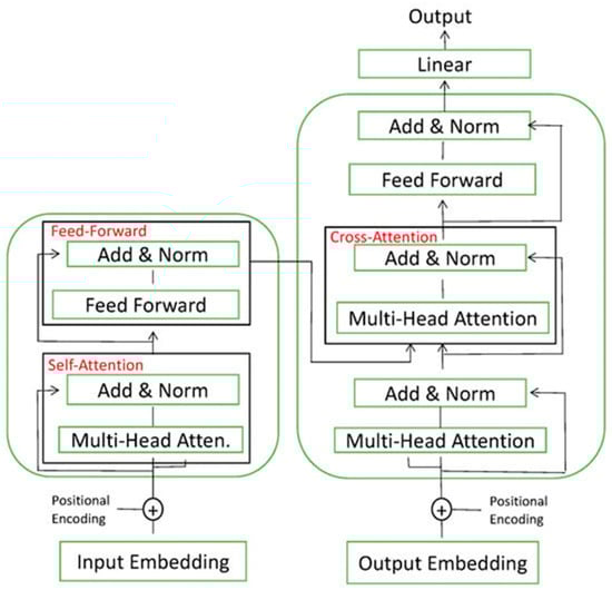
Figure 1.
Transformer architecture.
2.2. Long Short-Term Memory (LSTM) Networks
In the realm of time series prediction, traditional models like autoregressive models are the most utilized. These models are designed for adaptability, tailored individually to each time series, requiring human input to discern trends, seasonality and other patterns. In their studies, Salinas et al. [] discuss the adoption of RNNs as an alternative to classic techniques, with particular emphasis on long short-term memory (LSTM) networks. Despite their ability to retain memory states, LSTMs still encounter challenges in capturing long-term dependencies within the sequence of input data.
The LSTM model was proposed by Hochreiter and Schmidhuber [] and consists of a short-term memory network that is endowed with the capacity to store information from previous iterations of the network, i.e., previous states, allowing the network to combine this memory with new information to perform the calculation of the next state.
The use of this type of network for time series prediction has been widely studied in the literature; for a review, see, e.g., [,,]. The research developed by Malhotra [] studied the ability of LSTM networks to detect alternations in time series, allowing more robust predictions even in data with outliers. Along the same lines, Laptev [] discovered that neural networks could increase their efficiency compared to traditional methods when dealing with time series with high correlation and a large number of observations.
In LSTM networks, the cells (neurons) are endowed with a certain memory to record the data they received in the past. Figure 2 shows the inner structure of a single neuron. At time t, it receives new external data (xt) and the outputs of other neurons in the same layer (yt−1), which are processed along with the recorded information (ct−1) to provide a prediction as an output. There are three gates in the neuron: input gate, forget gate and output gate, to control the data flow.
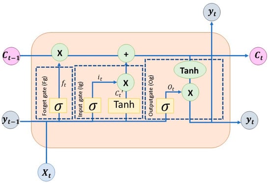
Figure 2.
LSTM architecture for a cell. The circles with “x” represent multiplication of their inputs, while those with “+” represent summation.
The past recorded information (memory) is represented with the variable c(t−1), which is updated in each time step to a new memory state ct. To better understand the time evolution of variables in an LSTM cell, variables that evolve with time show this fact with a subscript.
The ability to store or forget is regulated by the doors that make up the cell, allowing information to be added or deleted to memory at a given time. They perform the weighted sum of inputs to the neuron and feedback from other neurons in the same layer processed by a sigmoid activation function. A result of 0 in the sigmoid operation would imply not letting the information pass. An LSTM cell has three of these gates to control the state of the memory.
The forget door will decide which information should remain and which should be forgotten. This is achieved thanks to a sigmoid function, which has a range from 0 to 1, showing the relevance of the information in that range. In this gate, new inputs xt are processed along with the outputs of all neurons in the layer in the previous time step, yt−1, as a whole to decide whether the memory state should be modified or not:
In the previous formula, ft is the forget gate at time step t, which determines how much of the information from the memory cell of the previous time step ct−1 should be retained or discarded depending on the current inputs xt and previous outputs yt−1. Wf represents the weight vector (it is worth noting that in the neural network literature, weights are represented by matrices when referring to all neurons in a layer so that each row corresponds to a particular neuron. Since in this description, only one neuron is considered for simplicity, the corresponding weights are vectors (the row of a weight matrix). However, to be consistent with the convention used in the neural network literature, they are presented as matrices with a single row) associated with the forget gate, σ() denotes the sigmoid activation function used to regulate the output of the forget gate, and bf represents the corresponding bias.
The input door decides whether to update the inner state of the cell (its “memory”) with new inputs or not. The amount of information to be stored is determined by a sigmoid function, which provides values between 0 and 1. The information to be added to the cell “memory” is provided by a hyperbolic tangent activation function that processes the weighted sum of the new information provided to the cell and that arriving from other neurons in the same layers (feedback). This is the information that is added to the inner state, ct−1, once the input door allows it to enter the cell “memory”. The two results are combined to define a new inner state ct. The input door and the information to be added are as follows:
In the formulas provided, it represents the input gate at time step t, which controls how much new information is added to the cell state. It is calculated by the sigmoid activation function σ() applied to the weighted sum of the layer outputs at time t − 1, yt−1, and the current inputs xt, with Wi denoting the weight vector associated with the input gate and bi representing a bias term.
Similarly, ct′ represents the candidate cell state at time step t, which is a proposal for the new cell state. It is computed by applying the hyperbolic tangent function tanh() to the weighted sum of the layer outputs at time t − 1, yt−1, and the current inputs xt, with Wc representing the weight vector associated with the candidate cell state and bc denoting a bias term.
The new inner state will have the following form:
In this formula, ct represents the current cell state at time step t. It is computed by combining the previous cell state ct−1 with the candidate cell state ct′ weighted by the input gate it and the forget gate ft. This operation determines how much of the information from the previous cell state should be retained, how much new information should be added and how much should be forgotten.
The output gate is responsible for deciding what fraction of the inner state is provided as cell output. This inner state is processed by a hyperbolic tangent function before being released to compress its values between −1 and 1 in order to prevent the values from increasing or decreasing excessively, thus avoiding gradient fading problems during training:
In formula (6), ot represents the output gate at time step t, which regulates how much of the cell inner state ct is used to provide the output yt. It is calculated using the sigmoid activation function σ() applied to the weighted sum of the previous output yt−1 and the current input xt, with Wo representing the weight vector associated with the output gate and bo denoting the corresponding bias term.
Similarly, in formula (7), yt denotes the current cell output at time step t, which is calculated by multiplying the output gate ot by the hyperbolic tangent of the current cell state ct. This operation determines how much of the cell inner state is provided as the cell output.
2.3. Bidirectional LSTM (BiLSTM) Networks
The so-called bidirectional LSTM (BiLSTM) networks differ from LSTM in their model, intended to allow double training since the inputs are processed in a positive time direction (forward states) and in a negative time direction (backward states).
The research carried out by Siami-Namini et al. [] revealed to what extent it is beneficial to add additional layers to the training models, resulting in better results of the BiLSTM model compared to the LSTM thanks to the double training. These results are consistent with those reported by Kim and Moon in [], where they made predictions using a neural network based on a commercial time series.
The behavior of the BiLSTM model is shown in Figure 3, where three time steps are represented. The structure of the LSTM appears simplified to better understand the time evolution of the data traveling forward and backward. The model has two layers: one for the forward direction and the other for the backward direction. The inputs (xt) in time step t enter both the forward layer and the backward layer by means of weight matrices W1 and W3. In addition, both layers feedback to themselves their previous inner states ct−1 and c’t−1 by means of weight matrices W2 and W5. Then, both layers send their outputs to an output layer through matrices W4 and W6, which provides the model output as a combination of both responses.
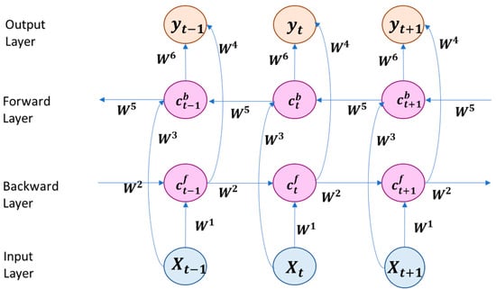
Figure 3.
BiLSTM architecture.
The formulas that describe the previous structure are as follows:
In the equations above, represents the inner states of the forward layer at time step t, which is determined by a function f() applied to the weighted sum of the current input xt and the previous inner states . This calculation involves two sets of weights, W1 for the input and W2 for the hidden state. Additionally, denotes the inner state of the backward layer at time step t, computed similarly to but using different weights, W3 for the input and W5 for the “following” inner state (this backward layer evolves backward in time). Finally, yt represents the output at time step t, determined by a function g() applied to the weighted sum of the current inner states and , with weights W4 and W6. The inner states are arranged in a vector made up of the inner states of all neurons in the corresponding forward and backward layers, so they are now in bold.
2.4. Multilayer Perceptron (MLP) Networks
Multilayer perceptron (MLP) models are composed of one input layer, one or several hidden layers and one output layer. Thanks to the use of backpropagation algorithms [], it is possible to train multilayer networks through a supervised approach by first calculating the error in the output layer and then adjusting weights in the previous layers in a backward iterative process. This process is carried out through supervised learning, in which both the input data and the expected output are provided to the network, which is responsible for making the corresponding association by adaptably adjusting the weights of all neurons in all layers to minimize the output error.
The multilayer perceptron is a feedforward type of network in which the inputs feed the network, propagating toward the outputs in a single direction, with the objective of sending the data from the input layer to the output layer and traversing all hidden layers that exist, which are responsible for processing the information and extracting the characteristic features.
It is one of the most studied models in the literature due to its simplicity []. The MLP model is efficient in prediction tasks given its great ability to establish relationships despite being the simplest model of those described. Currently, it is still the subject of many investigations [,].
In this model, the term “input layer” is used to refer to the data input, although technically it is not an actual layer. The output layer is defined to provide the output of the network. The layers between the input and output layers are known as hidden layers and carry out the processing of the information received by the network. The neurons in each layer receive connections from all neurons in the previous layer (or the inputs to the network for the first hidden layer). In this model, no feedback between neurons is defined, so MLPs perform pure feedforward processing of the information they receive. This means that the model does not consider any time dependence between the data it receives or the internal variables it calculates. Therefore, there are no references to time in the variables included in the equations that define the MLP structure.
The neurons in an MLP carry out very simple processing of the information they receive: a neuron j in a layer l receives all of the outputs of the previous layer, , which are multiplied by the weights that define the relationship between neuron j of layer l and neuron i of the layer l − 1. The output of the neuron, , is provided by an activation function f() of this weighted sum of its inputs plus a bias bj:
The activation function uses a sigmoid or hyperbolic tangent function in the hidden layers and a linear one in the output layer.
As an example, a network with one only hidden layer and one output is shown in Figure 4. To better understand this simple model, the outputs of the neurons in the hidden layer have been renamed to y = (y1, y2, y3, …, yN) and that of the output one to z (only one output). In that structure, x = (x1, x2, x3, …, xM) represents the input vector; wji (j = 1, 2, 3,…, N; i = 1, 2, 3, …, M) represents the weight matrix connecting the i-th element of the input vector with the j-th neuron of the hidden layer; and bj is the corresponding biases. The responses of these N neurons, y = (y1, y2, y3, …, yN), are as follows:
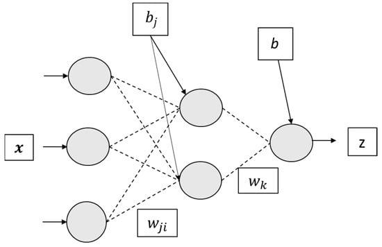
Figure 4.
MLP with one input layer, one hidden layer and an output layer.
The output of the only neuron, a linear function, of the output layer is as follows:
where wk defines the weights connecting the outputs of the neurons in the hidden layer with this one and b is a bias.
In these last two formulas, bj (j = 1, 2, 3, …, N) represents the biases of the neurons in the hidden layer and b that of the output neuron.
It is worth noting that MLPs are not recurrent networks, and, therefore, they are not time dependent, as LSTM and BiLSTM are. When dealing with time series, such as the problem at hand, these last two models receive one or more data points as input and process them along with past values recorded in their inner structures by means of recurrent connections between neurons, defining a time-dependent structure. However, this time dependence does not exist in MLPs and has to be simulated by presenting a set of past data as inputs to the model so that no explicit time dependence appears in the model. Therefore, when a time series is to be forecasted by an MLP, the input vector is a set of past data of the time series, which is processed to provide a prediction, i.e., the network receives at time t an input vector xt = (xt–1, xt–2, xt–3, …, xt–M), which is processed to provide a prediction (an output) zt. In order to properly perform this process, the time series should be rearranged into a matrix structure whose columns are these M-dimensional vectors, which are sequentially presented to the network to provide the corresponding prediction.
3. Experimentation
The final objective of this research is to identify an appropriate model to study economic time series. Despite being a topic widely researched in the literature, many of them have focused on testing and experimenting with the most recent models, increasing their complexity and processing times, which do not always imply a more accurate forecast, making them not the most suitable for analyzing this type of time series []. Therefore, we propose the use of four simple neural models (the models themselves without preprocessing or further modifications that provide complex forecasting structures) to forecast several time series to prove that simpler models are capable of providing not only accurate predictions but also predictions that can be better than those given by other complex models.
3.1. Datasets
In this section, the data used in the evaluation process of the ANNs used in this research (Transformers, LSTM, BiLSTM and MLP) will be described.
The first time series to study corresponds to the gold price index using the XAU/USD pair with daily data from 13 May 2015 to 15 June 2022, with a total of 1852 observations. The time series of the gold price, given its stationarity and volatility, is ideal for prediction with ANNs due to its non-linear patterns.
In order to carry out the contrast between the different models, it was essential to obtain other datasets with significant differences in behavior and number of observations, which is why the time series of electricity prices in the Spanish market, NEMO (Nominated Electricity Market Operator), will also be studied. It is used for market management by agents dealing with daily and intraday electricity prices. This time series is composed of 34,608 observations covering hourly intraday prices, hourly between 13 November 2019, and 24 October 2023. The complex patterns of this series, influenced by energy supply and demand, are suitable for prediction with neural networks, taking advantage of their ability to model non-linear relationships and capture market volatility.
The third dataset includes data from natural gas prices with 6821 observations between 7 January 1997, and 21 February 2024. The fluctuations that characterize this series, influenced by factors such as supply, demand and geopolitical events, require flexible models capable of capturing complex patterns for accurate prediction.
Finally, the results obtained by the time series corresponding to Brent oil prices are included in the comparison, which constitute a total of 9318 observations from 20 May 1987 to 5 February 2024.
The time series of Brent oil prices is also distinguished by its influence on global financial markets and its ability to reflect the global economic situation. This interconnection with other markets and economic sectors requires models with the ability to incorporate and model these complex relationships to improve the accuracy of predictions.
All data have been obtained through the Refinitv Eikon platform.
To carry out the experiments, it is necessary to normalize the data; this is a basic preprocessing step that allows for better fitting of the models’ metrics. The normalization of time series will accelerate the training process and facilitate the convergence of optimization algorithms, preventing potential bias in the case of significantly different scales, thereby ensuring greater fairness in the learning process. Max–min normalization offers results with greater precision than other models, which is why it has been chosen in this research.
In max–min normalization, the data are rescaled to a range between 0 and 1 according to the following equation, in which max(TS) and min(TS) are the maximum and minimum values of the original time series, respectively.
3.2. Error Metrics
In order to compare the accuracy of each model, four error metrics will be used in this work:
- -
- Root mean squared error (RMSE):
- -
- Mean squared error (MSE):
- -
- Mean absolute percentage error (MAPE):
- -
- R-squared (R2):where xt is the element of the time series at time t, while represents the corresponding predicted value, is the mean value of the time series, and T is the number of elements it has. The error in the predictions is measured using the MAPE and RMSE metrics, which allow us to know the adjustment of the neural network. Frechtling [] established optimal values for MAPE between 10% and 20% in predictions, while up to 30% could be considered acceptable. The ideal outcome is to have the lowest possible value as this will signify the smallest error in the predictions.
The MSE and R2 metrics are similar and allow us to assess the performance of the model by indicating the variation in the dependent variable based on the fit of the independent one. Better performance is reflected by a value as close to 1 as possible.
The use of R² as an additional metric to evaluate the fitting performance of non-linear models, complemented by other metrics such as MAPE, MSE and RMSE, allows for an intuitive and direct comparison with previous studies, facilitating the interpretation of results for a broader audience []. Although it is true that R² is traditionally used in the context of linear models, its application in non-linear models can provide valuable information about the proportion of variability explained by the model. R², being a widely recognized and understood metric, enhances the comprehensibility of the results. Additionally, the combined use of MAPE, MSE and RMSE ensures a robust and comprehensive evaluation of the model’s performance, addressing the potential limitations of R² by providing multiple perspectives on the model’s accuracy and error [].
3.3. Parameters
Tuning the hyperparameters of neural networks is fundamental to minimizing the risk of overfitting. The relevant parameters are as follows:
- -
- Learning rate: it is related to the number of epochs, since a value that is too low will make it necessary to increase the number of epochs and, as a consequence, result in slower training.
- -
- Batch size: it specifies the number of samples to be analyzed before updating the model parameters.
- -
- Epoch: it is the number of times the complete dataset will be trained in the model.
- -
- Optimization algorithm: This parameter can have a significant impact on the model since it will update the parameters based on the learning rate. In the experiments carried out in this research, Adam was used. This algorithm combines the benefits of RMSProp, which has certain similarities with gradient descent with momentum [].
- -
- num_heads: It represents the number of attention heads in the attention layer of the Transformer network. This model with a multi-head attention layer allows the network to focus on different parts of the input set simultaneously, while the number of heads controls how many different characteristics should be considered by the network when processing the information.
- -
- ff_dim: This parameter determines the dimension that the feedforward layer will have within the Transformer network structure. It is a dense layer that is applied after the care layer. The selection of this parameter will affect the network’s ability to perform learning with more complex patterns.
The research carried out by Goodfellow [] proposed recommendations on the optimal parameters to carry out predictions using neural networks, proposing a comparison using different options. The choice of parameters will be subject to computational limitations to avoid overfitting in the model. Table 1 lists the selected parameters for each of the models considered.

Table 1.
Selected parameters.
In order to better understand the architectures used, Table 2 and Table 3 describes in depth the hyperparameters used in the experiment.
Table 2.
Selected hyperparameters for BiLSTM, LSTM and MLP.
Table 3.
Selected hyperparameters for Transformer.
In their research, they established that the choice of parameters could be estimated as long as the parameters were not dependent on each other []. This assumption is possible as long as there are only a few parameters, since with a large number, the computational cost would grow exponentially. Smith pointed out that the error of an ANN can be minimized with an appropriate choice of hyperparameters, describing a new methodology that allowed eliminating the need to test with different values trying to find the maximum performance of the network [].
The use of 25 observations in the case of BiLSTM and LSTM recurrent neural networks allows for capturing data dependencies and patterns, allowing long-term behavior to be maintained [].
3.4. Experimentation Results
The four chosen time series are processed by the four artificial neural network models, selected for their proven effectiveness in fitting economic time series, showing great precision above other similar ones; for a review, see, e.g., [,].
Table 4 summarizes the main results of the four ANN models. The MLP network demonstrates more precise predictions by achieving a tighter fit of the next time sequence, resulting in lower values across all evaluation metrics (they are shown in bold in Table 4), highlighting its efficiency despite the inherent simplicity of this type of model.
Table 4.
Main results.
Achieving the best fit for the next observation allows us to reduce the complexity of the problem and simplify the results, making a more direct evaluation of the prediction capacity of each of the models [].
These results also suggest better performance of Transformer networks in time series with a large number of observations, as well as in those with fewer observations, where RNNs show less precise values due to the need to increase observations to improve the results.
The time series corresponding to the OMIE prices does not allow for obtaining a MAPE because the number of observations returns an inf value when trying to perform the division, since these are values very close to 0.
Figure 5, Figure 6, Figure 7 and Figure 8 graphically represent the results obtained by all of the models in each of the time series. In all cases, the fit obtained by the MLP model is superior to all of the others.
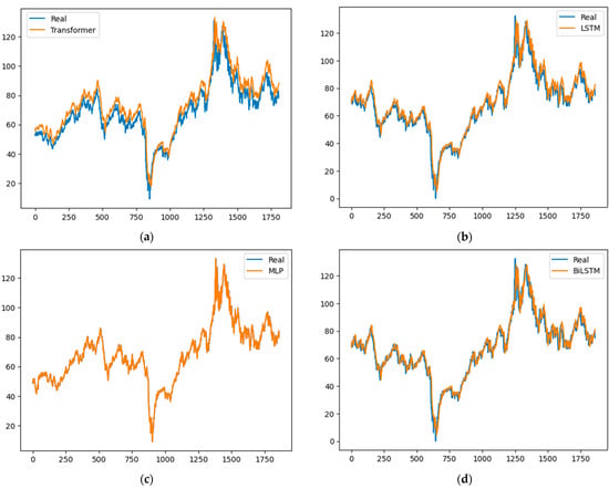
Figure 5.
Brent results: (a) Transformer, (b) LSTM, (c) MLP and (d) BiLSTM.
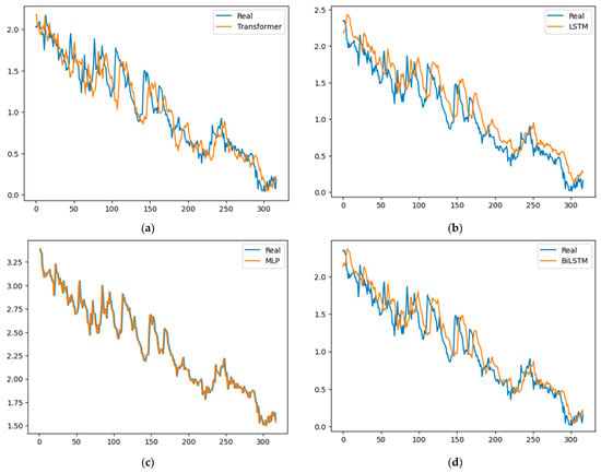
Figure 6.
Gold results: (a) Transformer, (b) LSTM, (c) MLP and (d) BiLSTM.
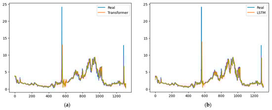
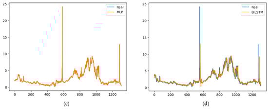
Figure 7.
GN results: (a) Transformer, (b) LSTM, (c) MLP and (d) BiLSTM.
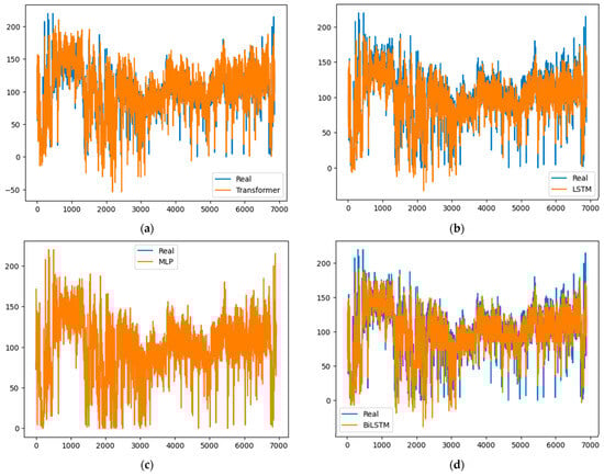
Figure 8.
OMIE results: (a) Transformer, (b) LSTM, (c) MLP and (d) BiLSTM.
These results show how a simple feedforward neural model (MLP) has been able to outperform both RNN models (LSTM and BILSTM) and Transformers, sophisticated neural models that have been shown to perform very complex tasks such as text identification and translation. RNNs and Transformers are widely used to forecast economic time series [,,,,,,], since they are able to extract and process relationships and dependencies among data organized in a sequence, the type of problem that text identification and translations represent, but they are also used for time series forecasting. They have been able to provide accurate and reliable predictions in this latter field, as the aforementioned works show; nevertheless, from a theoretical point of view, MLP could be considered more suitable for dealing with the problem of time series forecasting since it has been proved to be a universal approximator [], that is to say, it can approximate any continuous function provided that it has enough neurons. In addition, MLP is simpler and easier to program than RNN and Transformers.
It is difficult to compare the results presented in this work with those obtained in other papers because rarely were the exact same series used or the same error indices applied to measure accuracy. So, comparisons should be carried out only approximately. In this way, it may be seen in [] that a support vector regressor (SVR) combined with a decomposition technique of the series provided an accuracy only slightly better than that obtained in this work when forecasting oil prices; in [] also, oil prices were predicted with several deep learning neural models, and they all provided worse results than the MLP in the present work. In [], an SVR also provided worse results when forecasting gold prices; in [], several models (including an LSTM) were used to forecast natural gas prices, and they all performed worse than the MLP in the present work. These are just a few examples that prove that MLP can not only match the accuracy of other more sophisticated neural models in time series forecasting but in some cases can outperform them. Therefore, MLP is still widely studied as a reliable tool for forecasting [,,,].
4. Conclusions and Future Lines of Investigation
In this study, a comparative analysis of different deep learning models for time series forecasting was conducted. One key finding is that instead of assuming that modern techniques will yield more accurate results, simpler models that have been widely used in economic time series forecasting are recommended for reliable predictions. Four different time series were forecasted using four neural network models: Transformer, LSTM, MLP and BiLSTM. Transformers are complex and have been recently developed for generative AI tasks, producing impressive outcomes that have propelled AI to the forefront. LSTM and BiLSTM are recurrent neural networks, highly regarded in text analysis and translation, providing reliable tools and excellent predictions. MLP, a classic model, has been a fundamental network structure offering dependable solutions for regression and classification challenges, thus becoming a staple in time series forecasting.
The results obtained in this work show that sometimes, it is advisable to use simpler models to forecast time series, as they are able to provide significantly higher performance than more complex ones, since their simplicity allows for efficiently capturing the relationships between the data without the need to use recurrent models or with attention layers []. This is especially significant when forecasting univariate time series such as those analyzed in this work, where the identification of very complex patterns among multivariate data strings is not required, the same type of problem where deep learning neural models such as the three used in this work have provided astonishingly accurate results. A simple MLP is better suited to deal with a univariate regression problem of the type studied in this work than more complex models, as the results presented in this work show. Nevertheless, this result should not be surprising as the MLP has been proven to be a universal approximation [], since it can approximate any continuous function with one hidden layer provided that it has enough neurons. Therefore, several forecasting tools should be tested on a given time series to find out the best option []. As a rule of thumb, it may be stated that datasets with simple relationships between the data will be better processed with simple forecasting models, while those with very complex relationships will require complex forecasting models.
The results obtained in this work suggest further research in the study of the characteristics that make the use of one or another model ideal for prediction depending on the type of time series to be processed.
Author Contributions
Conceptualization, A.L., M.A.J.-M. and J.E.S.; methodology: A.L., M.A.J.-M. and J.E.S.; software, A.L.; validation: A.L., M.A.J.-M. and J.E.S.; formal analysis: A.L., M.A.J.-M. and J.E.S.; investigation: A.L., M.A.J.-M. and J.E.S.; resources: A.L., M.A.J.-M. and J.E.S.; data curation: A.L., M.A.J.-M. and J.E.S.; writing—original draft preparation, A.L., M.A.J.-M. and J.E.S.; writing—review and editing: A.L., M.A.J.-M. and J.E.S.; visualization, A.L., M.A.J.-M. and J.E.S.; supervision: A.L., M.A.J.-M. and J.E.S.; project administration: A.L., M.A.J.-M. and J.E.S. All authors have read and agreed to the published version of the manuscript.
Funding
This work was supported in part by the project TED2021-131671B-I00 funded by MCIN/AEI /10.13039/501100011033 and by the European Union NextGenerationEU/ PRTR.
Data Availability Statement
Restrictions apply to the availability of these data. Data were obtained from Thomson Eikon Reuters and are available from the Refinitiv application with the permission of Thomson Eikon Reuters. The code is available at: https://github.com/Analazcano/MLPvsTransformer.git (accessed on 1 March 2024).
Conflicts of Interest
The authors declare no conflicts of interest.
References
- Borghi, P.H.; Zakordonets, O.; Teixeira, J.P. A COVID-19 time series forecasting model based on MLP ANN. Procedia Comput. Sci. 2021, 181, 940–947. [Google Scholar] [CrossRef] [PubMed]
- Chen, S.A.; Li, C.L.; Yoder, N.; Arik, S.O.; Pfister, T. TSMixer: An All-MLP Architecture for Time Series Forecasting. arXiv 2023, arXiv:2303.06053. [Google Scholar]
- Voyant, C.; Nivet, M.L.; Paoli, C.; Muselli, M.; Notton, G. Meteorological time series forecasting based on MLP modelling using heterogeneous transfer functions. J. Phys. Conf. Ser. 2015, 574, 012064. [Google Scholar] [CrossRef]
- Shiblee, M.; Kalra, P.K.; Chandra, B. Time Series Prediction with Multilayer Perceptron (MLP): A New Generalized Error Based Approach. In Advances in Neuro-Information Processing; Köppen, M., Kasabov, N., Coghill, G., Eds.; Springer: Berlin/Heidelberg, Germany, 2009; pp. 37–44. [Google Scholar]
- Kamijo, K.; Tanigawa, T. Stock price pattern recognition-a recurrent neural network approach. In Proceedings of the 1990 IJCNN International Joint Conference on Neural Networks, San Diego, CA, USA, 17–21 June 1990; Volume 1, pp. 215–221. Available online: https://ieeexplore.ieee.org/abstract/document/5726532 (accessed on 18 March 2024).
- Chakraborty, K.; Mehrotra, K.; Mohan, C.K.; Ranka, S. Forecasting the behavior of multivariate time series using neural networks. Neural Netw. 1992, 5, 961–970. [Google Scholar] [CrossRef]
- de Rojas, A.L.; Jaramillo-Morán, M.A.; Sandubete, J.E. EMDFormer model for time series forecasting. AIMS Math. 2024, 9, 9419–9434. [Google Scholar] [CrossRef]
- Box, G.E.P.; Jenkins, G.M.; Reinsel, G.C.; Ljung, G.M. Time Series Analysis: Forecasting and Control; John Wiley & Sons: Hoboken, NJ, USA, 2015; pp. 88–126. ISBN 978-111-867-4925. [Google Scholar]
- Zerveas, G.; Jayaraman, S.; Patel, D.; Bhamidipaty, A.; Eickhoff, C. A Transformer-based Framework for Multivariate Time Series Representation Learning. In Proceedings of the 27th ACM SIGKDD Conference on Knowledge Discovery & Data Mining, New York, NY, USA, 14–18 August 2021. [Google Scholar]
- Wen, Q.; Zhou, T.; Zhang, C.; Chen, W.; Ma, Z.; Yan, J.; Sun, L. Transformers in Time Series: A Survey. arXiv 2023, arXiv:2202.07125. [Google Scholar]
- Zeng, A.; Chen, M.; Zhang, L.; Xu, Q. Are Transformers Effective for Time Series Forecasting? Proc. AAAI Conf. Artif. Intell. 2023, 37, 11121–11128. [Google Scholar] [CrossRef]
- Ahmed, S.; Nielsen, I.E.; Tripathi, A.; Siddiqui, S.; Ramachandran, R.P.; Rasool, G. Transformers in Time-Series Analysis: A Tutorial. Circuits Syst. Signal Process. 2023, 42, 7433–7466. [Google Scholar] [CrossRef]
- Sezer, O.B.; Gudelek, M.U.; Ozbayoglu, A.M. Financial time series forecasting with deep learning: A systematic literature review: 2005–2019. Appl. Soft Comput. 2020, 90, 106181. [Google Scholar] [CrossRef]
- Krollner, B.; Vanstone, B.; Finnie, G. Financial time series forecasting with machine learning techniques: A survey. Comput. Intell. 2010, 8, 25–30. [Google Scholar]
- Zhang, G.; Qi, M. Neural network forecasting for seasonal and trend time series. Eur. J. Oper. Res. 2005, 160, 501–514. [Google Scholar] [CrossRef]
- Hornik, K.; Stinchcombe, M.; White, H. Multilayer feedforward networks are universal approximators. Neural Netw. 1989, 2, 359–366. [Google Scholar] [CrossRef]
- Hill, T.; O’Connor, M.; Remus, W. Neural Network Models for Time Series Forecasts. Manag. Sci. 1996, 42, 1082–1092. [Google Scholar] [CrossRef]
- Khashei, M.; Bijari, M. An artificial neural network (p,d,q) model for timeseries forecasting. Expert Syst. Appl. 2010, 37, 479–489. [Google Scholar] [CrossRef]
- Bhardwaj, S.; Chandrasekhar, E.; Padiyar, P.; Gadre, V.M. A comparative study of wavelet-based ANN and classical techniques for geophysical time-series forecasting. Comput. Geosci. 2020, 138, 104461. [Google Scholar] [CrossRef]
- Di Piazza, A.; Di Piazza, M.C.; La Tona, G.; Luna, M. An artificial neural network-based forecasting model of energy-related time series for electrical grid management. Math Comput. Simul. 2021, 184, 294–305. [Google Scholar] [CrossRef]
- Kumar, B.; Sunil Yadav, N. A novel hybrid model combining βSARMAβSARMA and LSTM for time series forecasting. Appl. Soft Comput. 2023, 134, 110019. [Google Scholar] [CrossRef]
- Devlin, J.; Chang, M.-W.; Lee, K.; Toutanova, K. BERT: Pre-Training of Deep Bidirectional Transformers for Language Understanding. arXiv 2018, arXiv:1810.04805. Available online: https://arxiv.org/abs/1810.04805 (accessed on 7 October 2020).
- Dosovitskiy, A.; Beyer, L.; Kolesnikov, A.; Weissenborn, D.; Zhai, X.; Unterthiner, T.; Dehghani, M.; Minderer, M.; Heigold, G.; Gelly, S.; et al. An Image is Worth 16x16 Words: Transformers for Image Recognition at Scale. arXiv 2021, arXiv:2010.11929. Available online: http://arxiv.org/abs/2010.11929 (accessed on 18 March 2024).
- Cholakov, R.; Kolev, T. Transformers predicting the future. Applying attention in next-frame and time series forecasting. arXiv 2021, arXiv:2108.08224. Available online: http://arxiv.org/abs/2108.08224 (accessed on 19 March 2024).
- Lim, B.; Arık, S.; Loeff, N.; Pfister, T. Temporal Fusion Transformers for interpretable multi-horizon time series forecasting. Int. J. Forecast. 2021, 37, 1748–1764. [Google Scholar] [CrossRef]
- Wu, H.; Xu, J.; Wang, J.; Long, M. Autoformer: Decomposition Transformers with Auto-Correlation for Long-Term Series Forecasting. In Advances in Neural Information Processing Systems; Curran Associates, Inc.: New York, NY, USA, 2021; pp. 22419–22430. Available online: https://proceedings.neurips.cc/paper/2021/hash/bcc0d400288793e8bdcd7c19a8ac0c2b-Abstract.html (accessed on 19 March 2024).
- Zeyer, A.; Bahar, P.; Irie, K.; Schlüter, R.; Ney, H. A Comparison of Transformer and LSTM Encoder Decoder Models for ASR. In Proceedings of the 2019 IEEE Automatic Speech Recognition and Understanding Workshop (ASRU), Singapore, 14–18 December 2019; pp. 8–15. Available online: https://ieeexplore.ieee.org/abstract/document/9004025 (accessed on 19 March 2024).
- Vaswani, A.; Shazeer, N.; Parmar, N.; Uszkoreit, J.; Jones, L.; Gomez, A.N.; Kaiser, Ł.; Polosukhin, I. Attention is All you Need. In Advances in Neural Information Processing Systems; Curran Associates, Inc.: New York, NY, USA, 2017; Available online: https://proceedings.neurips.cc/paper_files/paper/2017/hash/3f5ee243547dee91fbd053c1c4a845aa-Abstract.html (accessed on 18 March 2024).
- Li, C.; Qian, G. Stock Price Prediction Using a Frequency Decomposition Based GRU Transformer Neural Net-work. Appl Sci. 2023, 13, 222. [Google Scholar] [CrossRef]
- Salinas, D.; Flunkert, V.; Gasthaus, J.; Januschowski, T. DeepAR: Probabilistic forecasting with autoregressive re-current networks. Int. J. Forecast. 2020, 36, 1181–1191. [Google Scholar] [CrossRef]
- Hochreiter, S.; Schmidhuber, J. Long Short-Term Memory. Neural Comput. 1997, 9, 1735–1780. [Google Scholar] [CrossRef] [PubMed]
- Sagheer, A.; Kotb, M. Time series forecasting of petroleum production using deep LSTM recurrent networks. Neurocomputing 2018, 323, 203–213. [Google Scholar] [CrossRef]
- Yamak, P.T.; Yujian, L.; Gadosey, P.K. A Comparison between ARIMA, LSTM, and GRU for Time Series Forecasting. In Proceedings of the 2019 2nd International Conference on Algorithms, Computing and Artificial Intelligence, Sanya, China, 20–22 December 2019. [Google Scholar]
- Siami-Namini, S.; Tavakoli, N.; Namin, A.S. The Performance of LSTM and BiLSTM in Forecasting Time Series. In Proceedings of the 2019 IEEE International Conference on Big Data (Big Data), Los Angeles, CA, USA, 9–12 December 2019; pp. 3285–3292. [Google Scholar] [CrossRef]
- Malhotra, P.; Ramakrishnan, A.; Anand, G.; Vig, L.; Agarwal, P.; Shroff, G. LSTM-based Encoder-Decoder for Multi-sensor Anomaly Detection. arXiv 2016, arXiv:1607.00148. Available online: http://arxiv.org/abs/1607.00148 (accessed on 19 March 2024).
- Laptev, N.; Yu, J.; Rajagopal, R. Applied timeseries Transfer learning. 2018. Available online: https://openreview.net/forum?id=BklhkI1wz (accessed on 19 March 2024).
- Kim, J.; Moon, N. BiLSTM model based on multivariate time series data in multiple field for forecasting trading area. J. Ambient. Intell. Humaniz. Comput. 2019, 1–10. [Google Scholar] [CrossRef]
- Rumelhart, D.E.; Hinton, G.E.; Williams, R.J. Learning representations by back-propagating errors. Nature 1986, 323, 533–536. [Google Scholar] [CrossRef]
- Zhang, T.; Zhang, Y.; Cao, W.; Bian, J.; Yi, X.; Zheng, S.; Li, J. Less Is More: Fast Multivariate Time Series Forecasting with Light Sampling-oriented MLP Structures. arXiv 2022, arXiv:2207.01186. Available online: http://arxiv.org/abs/2207.01186 (accessed on 4 March 2024).
- Yi, K.; Zhang, Q.; Fan, W.; Wang, S.; Wang, P.; He, H.; Lian, D.; An, N.; Cao, L.; Niu, Z. Frequency-domain MLPs are More Effective Learners in Time Series Forecasting. Adv. Neural Inf. Process Syst. 2023, 36, 76656–76679. [Google Scholar]
- Madhusudhanan, K.; Jawed, S.; Schmidt-Thieme, L. Hyperparameter Tuning MLPs for Probabilistic Time Series Forecasting. arXiv 2024, arXiv:2403.04477. Available online: http://arxiv.org/abs/2403.04477 (accessed on 19 March 2024).
- Shen, F.; Chao, J.; Zhao, J. Forecasting exchange rate using deep belief networks and conjugate gradient method. Neurocomputing 2015, 167, 243–253. [Google Scholar] [CrossRef]
- Frechtling, D. Forecasting Tourism Demand; Routledge: London, UK, 2001; 279p. [Google Scholar]
- Olawoyin, A.; Chen, Y. Predicting the Future with Artificial Neural Network. Procedia Comput. Sci. 2018, 140, 383–392. [Google Scholar] [CrossRef]
- Pierce, D.A. R 2 Measures for Time Series. J. Am. Stat. Assoc. 1979, 74, 901–910. [Google Scholar] [CrossRef]
- Sun, R. Optimization for deep learning: Theory and algorithms. arXiv 2019, arXiv:1912.08957. Available online: http://arxiv.org/abs/1912.08957 (accessed on 24 March 2024).
- Goodfellow, I.; Pouget-Abadie, J.; Mirza, M.; Xu, B.; Warde-Farley, D.; Ozair, S.; Courville, A.; Bengio, Y. Generative adversarial networks. Commun ACM. 2020, 63, 139–144. [Google Scholar] [CrossRef]
- Beck, J.V.; Arnold, K.J. Parameter Estimation in Engineering and Science; Wiley: Hoboken, NY, USA, 1977; 540p. [Google Scholar]
- Smith, L.N. A disciplined approach to neural network hyper-parameters: Part 1-learning rate, batch size, momentum, and weight decay. arXiv 2018, arXiv:1803.09820. Available online: http://arxiv.org/abs/1803.09820 (accessed on 24 March 2024).
- Pirani, M.; Thakkar, P.; Jivrani, P.; Bohara, M.H.; Garg, D. A Comparative Analysis of ARIMA, GRU, LSTM and BiLSTM on Financial Time Series Forecasting. In Proceedings of the 2022 IEEE International Conference on Distributed Computing and Electrical Circuits and Electronics (ICDCECE), Ballari, India, 23–24 April 2022; pp. 1–6. [Google Scholar]
- Yang, M.; Wang, J. Adaptability of Financial Time Series Prediction Based on BiLSTM. Procedia Comput. Sci. 2022, 199, 18–25. [Google Scholar] [CrossRef]
- Xiong, T.; Bao, Y.; Hu, Z. Beyond one-step-ahead forecasting: Evaluation of alternative multi-step-ahead forecasting models for crude oil prices. Energy Econ. 2013, 40, 405–415. [Google Scholar] [CrossRef]
- Fan, L.; Pan, S.; Li, Z.; Li, H. An ICA-based support vector regression scheme for forecasting crude oil prices. Technol. Forecast. Soc. Chang. 2016, 112, 245–253. [Google Scholar] [CrossRef]
- Aldabagh, H.; Zheng, X.; Mukkamala, R. A Hybrid Deep Learning Approach for Crude Oil Price Prediction. J. Risk Financ. Manag. 2023, 16, 503. [Google Scholar] [CrossRef]
- Prediction of Gold Price with ARIMA and SVM—IOPscience. Available online: https://iopscience.iop.org/article/10.1088/1742-6596/1767/1/012022/meta (accessed on 12 May 2024).
- Wang, J.; Lei, C.; Guo, M. Daily natural gas price forecasting by a weighted hybrid data-driven model. J. Pet. Sci. Eng. 2020, 192, 107240. [Google Scholar] [CrossRef]
- Fildes, R.; Petropoulos, F. Simple versus complex selection rules for forecasting many time series. J. Bus. Res. 2015, 68, 1692–1701. [Google Scholar] [CrossRef]
Disclaimer/Publisher’s Note: The statements, opinions and data contained in all publications are solely those of the individual author(s) and contributor(s) and not of MDPI and/or the editor(s). MDPI and/or the editor(s) disclaim responsibility for any injury to people or property resulting from any ideas, methods, instructions or products referred to in the content. |
© 2024 by the authors. Licensee MDPI, Basel, Switzerland. This article is an open access article distributed under the terms and conditions of the Creative Commons Attribution (CC BY) license (https://creativecommons.org/licenses/by/4.0/).