Abstract
Addressing the issues of the sand cat swarm optimization algorithm (SCSO), such as its weak global search ability and tendency to fall into local optima, this paper proposes an improved strategy called the multi-strategy integrated sand cat swarm optimization algorithm (MSCSO). The MSCSO algorithm improves upon the SCSO in several ways. Firstly, it employs the good point set strategy instead of a random strategy for population initialization, effectively enhancing the uniformity and diversity of the population distribution. Secondly, a nonlinear adjustment strategy is introduced to dynamically adjust the search range of the sand cats during the exploration and exploitation phases, significantly increasing the likelihood of finding more high-quality solutions. Lastly, the algorithm integrates the early warning mechanism of the sparrow search algorithm, enabling the sand cats to escape from their original positions and rapidly move towards the optimal solution, thus avoiding local optima. Using 29 benchmark functions of 30, 50, and 100 dimensions from CEC 2017 as experimental subjects, this paper further evaluates the MSCSO algorithm through Wilcoxon rank-sum tests and Friedman’s test, verifying its global solid search ability and convergence performance. In practical engineering problems such as reducer and welded beam design, MSCSO also demonstrates superior performance compared to five other intelligent algorithms, showing a remarkable ability to approach the optimal solutions for these engineering problems.
Keywords:
the good point set strategy; nonlinear adjustment strategy; vigilance mechanism fused with sparrow algorithm; engineering applications MSC:
58-04
1. Introduction
Optimization problems refer to finding the optimal solution from all possible scenarios under certain conditions, aiming to maximize or minimize performance indicators. These problems are primarily applied in practical engineering applications [1], image processing [2], path planning [3], and other fields.
Engineering optimization problems aim to solve real-life problems with constraints, enabling engineering systems’ parameters to reach their optimal states. During the development of the engineering field, numerous nonlinear and high-dimensional problems have emerged, making optimization problems increasingly complex, with corresponding increases in computational complexity. Traditional optimization algorithms were widely developed and applied to various optimization problems in the early stages. However, traditional optimization algorithms have certain limitations regarding problem form and scale. They face challenges such as high computational costs and slow convergence speeds for complex or large-scale problems, making it challenging to find the optimal solution within a reasonable time frame.
Metaheuristic algorithms have demonstrated remarkable robustness in addressing the shortcomings of traditional optimization algorithms when dealing with complex problems. These complex issues encompass multi-objective, single-objective, discrete, combinatorial, high-dimensional, or dynamic optimization, among others [4]. Metaheuristic algorithms are general-purpose optimization algorithms characterized by their global perspective when searching the solution space [5]. They are primarily divided into four categories: evolutionary-based algorithms, swarm-based algorithms, algorithms inspired by physics, mathematics, and chemistry, and algorithms based on human and social behaviors [6]. This article primarily focuses on swarm-based algorithms, i.e., swarm intelligence optimization algorithms, which mimic the behavior of natural swarms to achieve information exchange and cooperation, ultimately identifying the optimal solution to optimization problems. From early algorithms such as particle swarm optimization (PSO) [7], ant colony optimization (ACO) [8], and genetic algorithm (GA) [9] to later developments including the sparrow search algorithm (SSA) [10], dung beetle optimizer (DBO) [11], pelican optimization algorithm (POA) [12], Harris hawks optimization (HHO) [13], and subtraction-average-based optimization (SABO) [14], swarm intelligence optimization algorithms have gradually evolved into an optimization method with few design parameters and simple operation.
The sand cat swarm optimization (SCSO) algorithm is a novel swarm intelligence optimization algorithm, proposed by Seyyedabbasi in 2022 [15], inspired by the behavior of sand cats in nature. The SCSO algorithm is divided into an exploration phase and an exploitation phase, with the balance between the two phases adjusted by the parameter R. Due to its robust and powerful optimization capabilities, SCSO has been widely applied in various fields. For instance, it has been used to predict the scale of short-term rock burst damage [16] and design feedback controllers for nonlinear systems [17]. Nevertheless, the SCSO algorithm also has some drawbacks, such as slow convergence speed, poor global search ability during the exploration phase, and a tendency to fall into local optima.
Various experts and scholars have proposed improvements to address these shortcomings of the SCSO algorithm. Ref. [18] combined dynamic pinhole imaging and the golden sine algorithm to enhance the optimization performance of the sand cat population, improving global search ability through dynamic pinhole imaging and enhancing exploitation ability and convergence through the golden sine algorithm. Ref. [19] utilized a target encoding mechanism, elitism strategy, and adaptive T-distribution to solve dynamic path-planning problems, improving path-planning efficiency and introducing the ability to escape local optima. Ref. [20] proposed combining SCSO with reinforcement learning techniques to improve the algorithm’s ability to find optimal solutions in a given search space. Ref. [21] used chaotic mapping with chaos concepts to enhance global search ability and reduce issues like slow transitions between phases and early or late convergence. Ref. [22] defined a new coefficient affecting the exploration and exploitation phases and introduced a mathematical model to address the issues of slow convergence and late exploitation issues in SCSO. Although the experts and scholars above have significantly improved the SCSO algorithm’s performance, some areas still need further improvement, as shown in Table 1.

Table 1.
Improved SCSO.
In summary, while specific improvements have been made in the literature to address the shortcomings of the SCSO algorithm, according to the no free lunch theorem [23], despite the extensive research and enhancements made to the SCSO algorithm’s global search ability, convergence performance, and ability to escape local optima, existing optimization strategies are still insufficient to tackle the ever-changing and increasing complexity of real-world problems. Therefore, it is necessary to continue improving the SCSO algorithm.
To further optimize the SCSO algorithm’s performance and expand its applications in engineering problems, this paper proposes a multi-strategy fusion sand cat swarm optimization (MSCSO) algorithm.
- During the initial population phase, the good point set strategy is adopted to ensure the population is evenly distributed within the search space, enhancing population diversity.
- A nonlinear adjustment strategy is introduced in the exploration phase to improve the sand cat’s sensitivity range, dynamically adjusting the balance conversion parameters between the exploration and exploitation stages.it expands the search range of the sand cats, enhances the algorithm’s global search ability, and reduces the risk of falling into local optima.
- In the exploitation phase, the sparrow search algorithm’s warning mechanism is fused to update the sand cats’ positions, enabling them to respond quickly when approaching optimality, avoid falling into local optima, and accelerate the algorithm’s convergence speed.
2. SCSO: Sand Cat Swarm Optimization Algorithm
2.1. Population Initialization
Sand cats are randomly generated in the search area, with the position of the individual as indicated in Equation (1).
where the and represent the upper and lower limits of the search area. is a random number between 0 and 1, and d is the dimensionality of the algorithm. The upper and lower bounds of the search area are as shown in Equation (2).
2.2. Search for Prey (Exploration Phase)
In the exploration stage, the sand cat’s search behavior and attack behavior were dynamically adjusted by changing the size of the R-value, as shown in Equation (4). When the |R| < 1, the sand cat performs a search behavior, and during the search process, the sand cat relies on the range of low-frequency noise to locate its prey, by effectively exploring the potential best prey locations with sand cat location updates, as Equation (6) indicates.
where the value drops linearly from 2 to 0, is the auditory feature with a value of 2, is the current number of updates, is the maximum number of updates, is a random number from 0 to 1, and is the sensitivity range [15].
where represents the current best location, and is the current location.
2.3. Attacking Prey (Development Phase)
When the |R| 1, the sand cat starts to attack, gradually narrowing down the search area to improve the search accuracy when approaching the prey. At this stage, the sand cat selects a random angle between 0 and 360 in the search area and uses and to generate a random position, making the sand cat’s attack behavior more flexible and changeable, increasing the probability of finding the global optimal solution, as Equation (8) indicates.
where is the optimal position and is the random position.
The pseudocode of SCSO is presented in Algorithm 1.
| Algorithm 1 SCSO |
| 1: Initialize the population |
| 2: Calculate the fitness function based on the objective function |
| 3: Use Equations (3)–(5) to initialize the parameters , R, and r |
| 4: while (t < T) do |
| 5: for Every individual do |
| 6: Take a random angle θ between 0 and 360° |
| 7: if |R| ≤ 1 |
| 8: Use Equation (8) to update the position |
| 9: else |
| 10: Use Equation (6) to update the location |
| 11: end |
| 12: end |
| 13: end |
3. MSCSO: Fusion of Multi-Strategy Sand Cat Swarm Optimization Algorithm
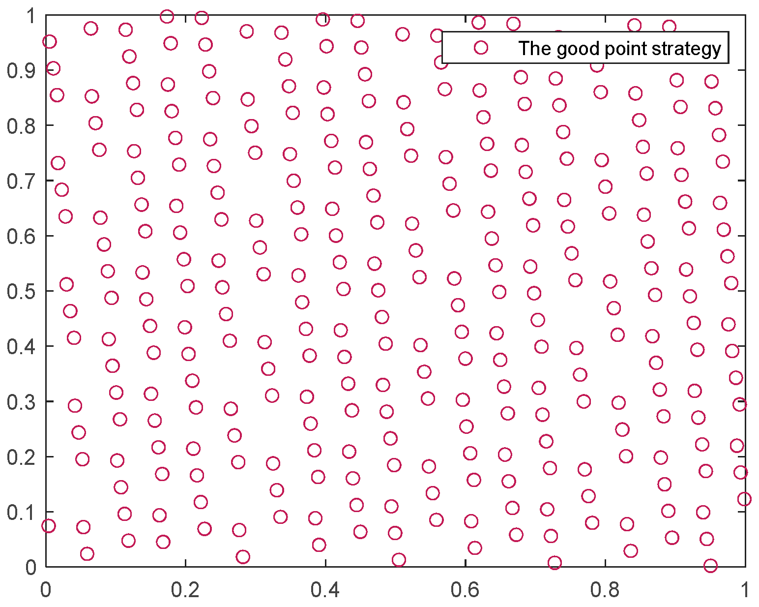
3.1. The Good Point Set Strategy
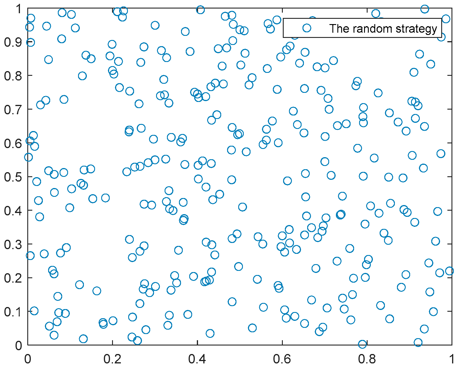
Based on Equation (1), it can be seen that the SCSO algorithm initializes the population using a random strategy, resulting in a random distribution of the population within the search space; it can lead to an uneven distribution of the population and an increased likelihood of falling into local optima. Therefore, this paper introduces the good point set strategy, which was proposed by Hua Luogeng in 1978. This strategy utilizes the distribution patterns of point sets to optimize search and solution efficiency [24]. Meanwhile, Ref. [25] employed the good point set strategy to distribute the population uniformly within the search space, effectively enhancing population diversity and reducing the probability of falling into local optima. Given the advantages of the good point set strategy in initializing populations, this paper adopts the good point set strategy for population initialization. The steps are as follows:
Step 1: Generate the smallest prime number within the z-dimensional Euclidean space, as Equation (9) depicts.
Step 2: Generate a good point within the z-dimensional space, as Equation (10) depicts.
Step 3: Let Gz be the unit cube in the z-dimensional Euclidean space, generating a good point set with a sample size of n, as Equation (11) depicts.
Step 4: Replace Equation (1) with Equation (12) for population initialization.
In a two-dimensional plane, 300 points were randomly generated using the good point set and random strategy, as shown in Figure 1 and Figure 2. Based on the distribution of these 300 points, it can be observed that the good point set strategy results in a more uniform distribution across the entire search space, enhancing the diversity of the SCSO algorithm; it validates the effectiveness of the good point set strategy in initializing the population for the SCSO algorithm.
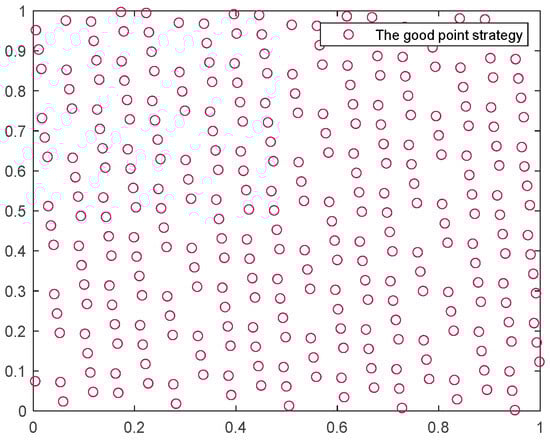
Figure 1.
The good point set strategy.
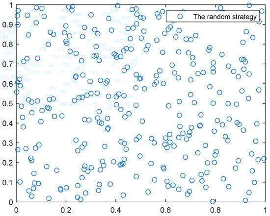
Figure 2.
The random strategy.
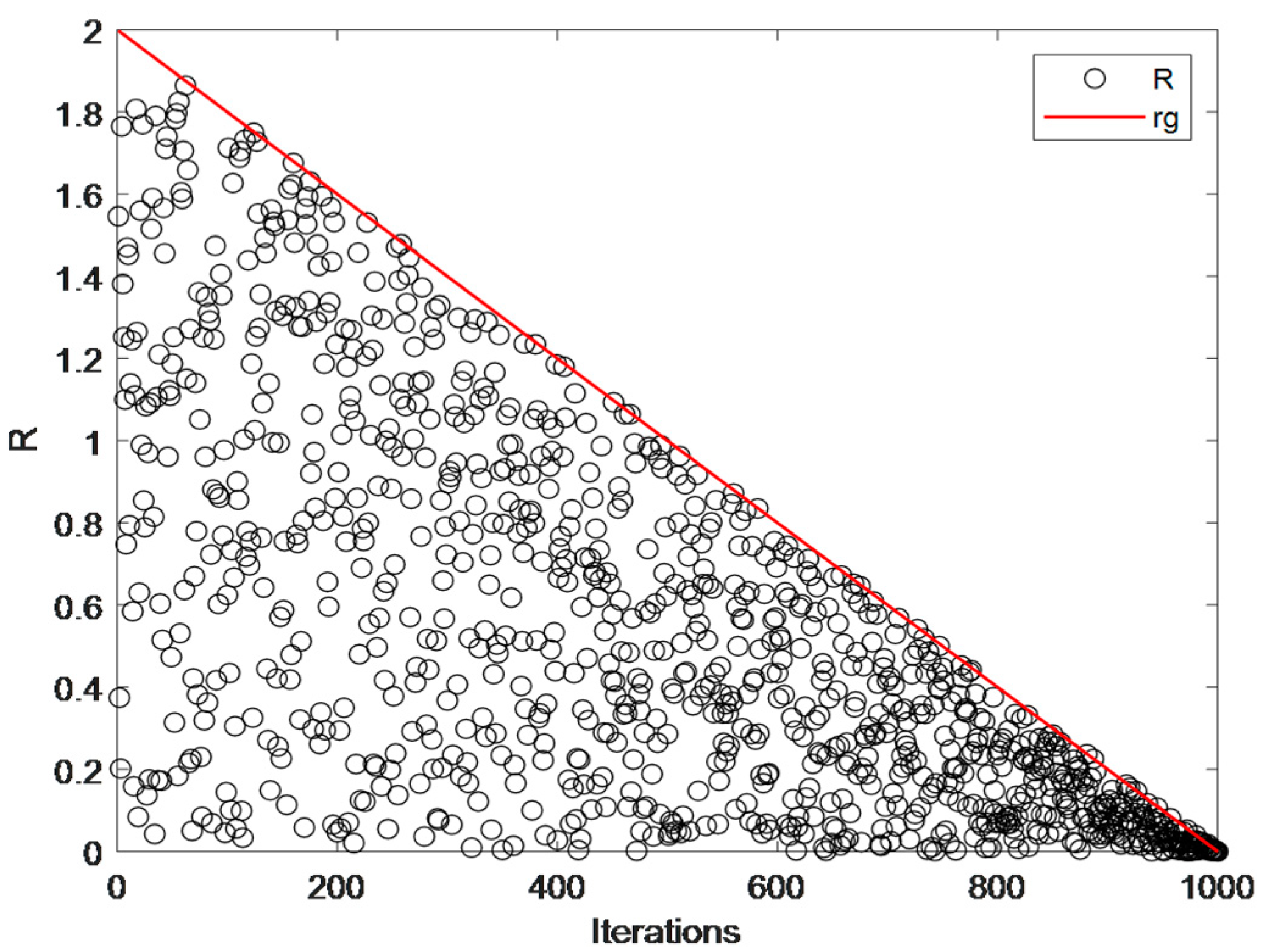
3.2. Nonlinear Adjustment Strategy
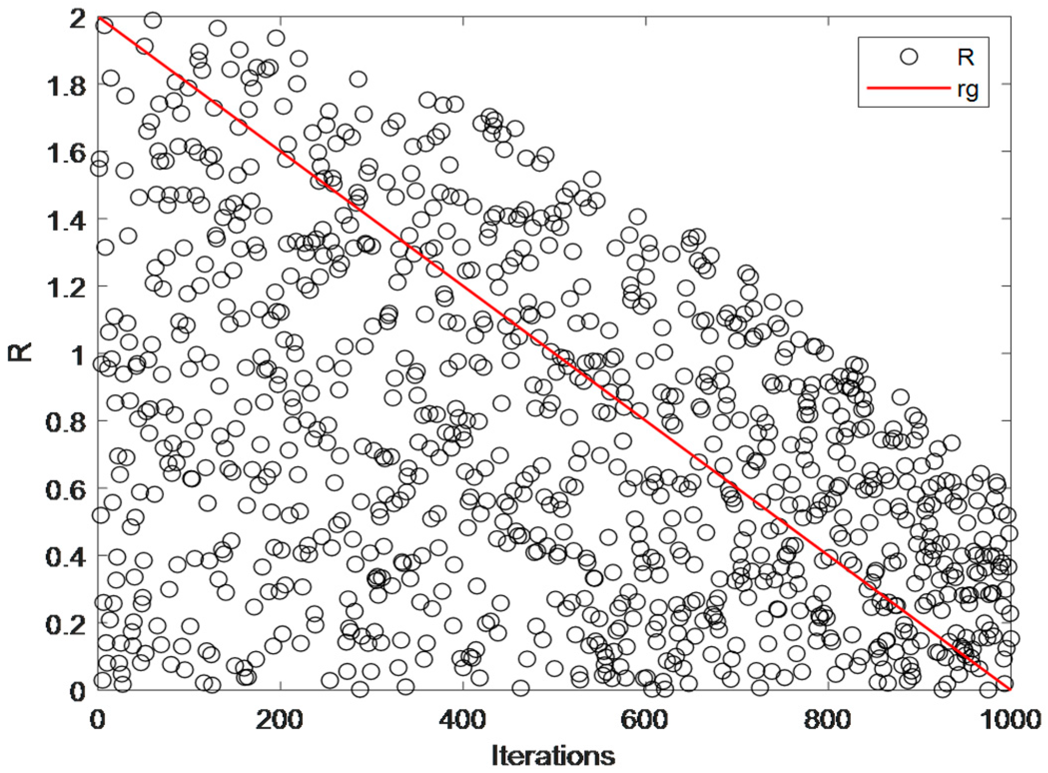
The SCSO algorithm prioritizes breadth during the exploration phase and emphasizes depth and speed during the exploitation phase. As indicated in Equation (3), the sensitivity range of the sand cat’s value gradually decreases linearly from 2 to 0. This linear decrease does not fully utilize the global search capability of Equation (3), resulting in a tendency for the algorithm to get trapped in local optima. Consequently, a nonlinear adjustment strategy is adopted to improve Equation (3). Studies in [26,27] have validated that transitioning from a linear method to a nonlinear adjustment strategy enables the algorithm to maintain both global search capability and local exploitation ability throughout the entire iteration process, thus fulfilling the algorithm’s requirements across iterations. In this paper, the improved nonlinear substitution formula for Equation (3) is utilized to modify the auditory range of the sand cat. The steps for enhancing the nonlinear adjustment strategy formula are outlined below. Additionally, the modified formula is presented as Equation (14).
Step 1: Design parameter f, as shown in Equation (13)
Step 2: Introduce f into the original Equation (3); the improved Equation is shown as Equation (14).
where the is the auditory feature with a value of 2, is the current number of updates, is the maximum number of updates.
As shown in Figure 3 and Figure 4, a comparative analysis was conducted on the search range capabilities of the linear and nonlinear adjustment strategies. The red line represents the process where changes linearly from 2 to 0, while the black line depicts the improved range. From the figures, it is evident that the exploitation phase of SCSO overly emphasizes local attacks, neglecting the global search capability. However, the improved formula enables extensive exploration during the exploration phase and facilitates both local attacks and global exploration during the exploitation phase. It can be concluded that Equation (14) significantly enhances the overall performance of the algorithm and reduces the risk of falling into local optima; it verifies the global search capability of the nonlinear adjustment strategy during the exploitation phase.

Figure 3.
The global search scope of Equation (3).
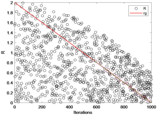
Figure 4.
The global search scope of Equation (14).
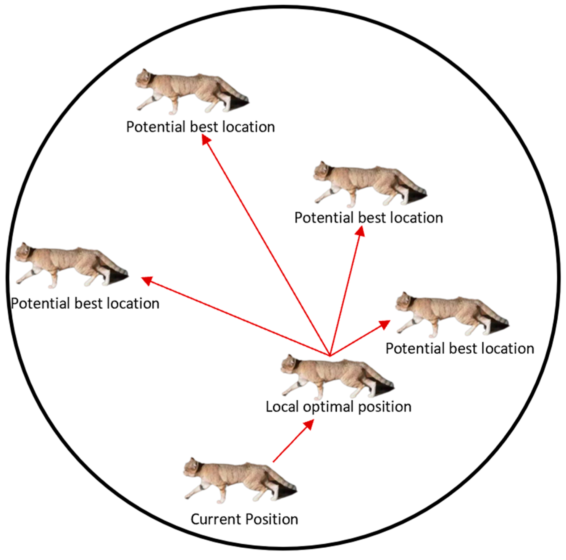
3.3. Integrate the Warning Mechanism of the Sparrow Algorithm
In the later iterations of the SCSO algorithm, the convergence speed may be relatively slow when dealing with some complex issues, requiring a longer computational time to find the optimal solution. The warning mechanism in the SSA can rapidly guide sparrows toward the optimal position based on their current locations [10], thereby enhancing the algorithm’s convergence during the iteration process and reducing computational time. Therefore, inspired by the sparrow search algorithm, this paper introduces the warning mechanism of the sparrow algorithm into the SCSO algorithm. The detailed position update Equation is shown in Equation (15).
where is the current global optimal position, indicates the worst position of the Tth iteration, is the step-size control parameter, ∈ [−1.1] is a random number, is the current fitness value, is the current global optimal fitness value, is the minimum fitness value of the current population, is constant [10]. The steps for updating the position are as follows.
Step 1: In the sand cat population, 30% of the individuals are randomly selected to serve as warning sand cats.
Step 2: While , this indicates that the sand cat is safe around , and it can randomly move within this range to avoid falling into a local optimum. The specific movement position of the sand cat is represented as .
Step 3: While , this indicates that the sand cat realizes it is in an unfavorable position and needs to move closer to other sand cats to find an optimal position. The sand cat updates its position according to the Equation . The sand cats’ position updates are illustrated in Figure 5.
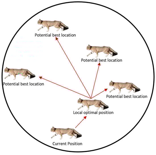
Figure 5.
Movement diagram of the warning mechanism of the sand cat fusion with sparrow algorithm.
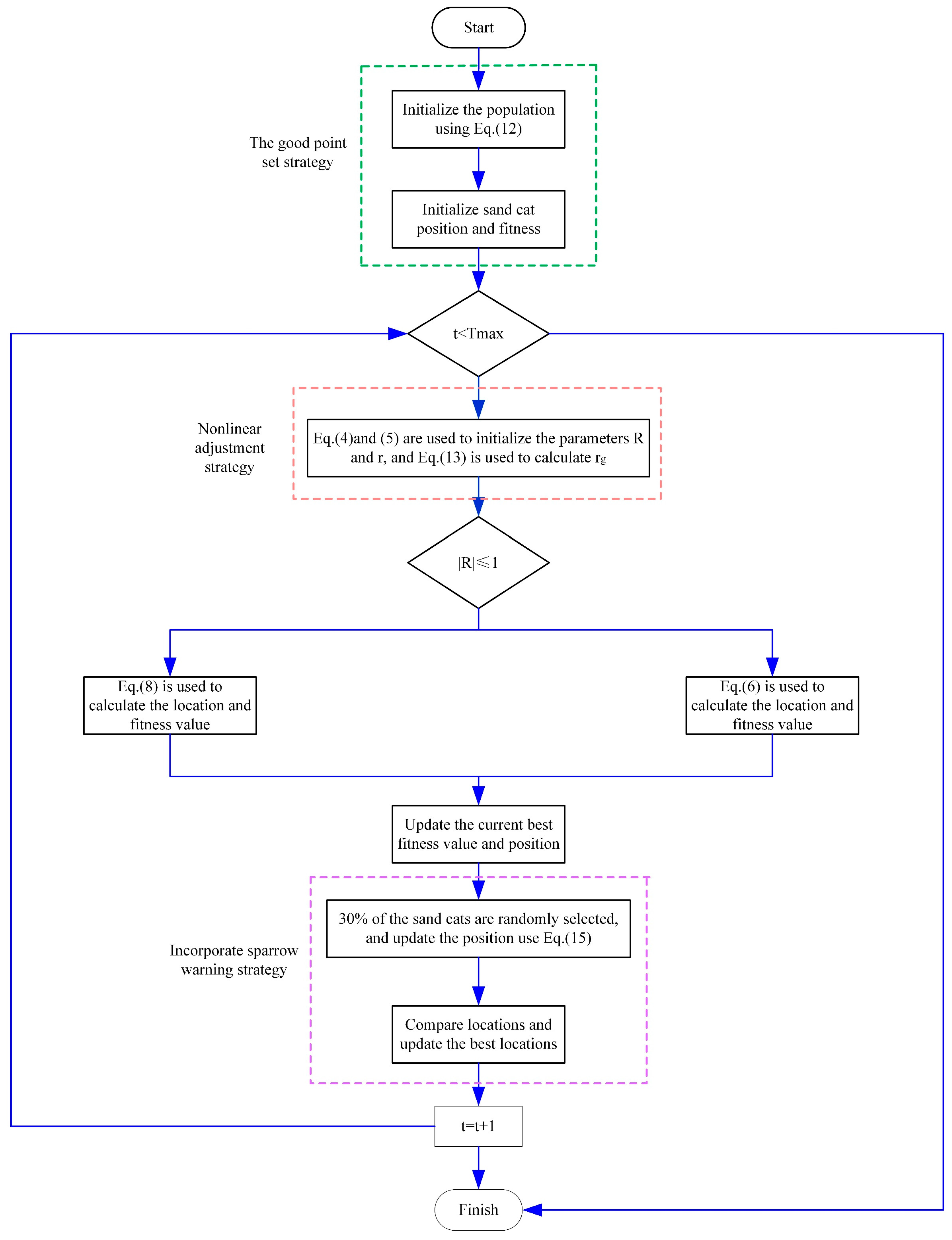
3.4. MSCSO Algorithm Flowchart and Pseudocode
Figure 6 shows the flow chart of the MSCSO algorithm after SCSO is integrated with the good point set strategy, the nonlinear adjustment strategy, and the early warning mechanism of the sparrow search algorithm. The MSCSO pseudocode is presented in Algorithm 2.
| Algorithm 2 MSCSO |
| Parameters: the current fitness value , the current global optimal fitness value |
| 1: Initialize the population using Equation (12) |
| 2: Calculate the location and fitness values for each individual |
| 3: Use Equations (4) and (5) are used to initialize the parameters R and r and Equation (13) is used to calculate R |
| 4: while (t < T) do |
| 5: for Every individual do |
| 6: Take a random angle θ between 0 and 360° |
| 7: if |R| ≤ 1 |
| 8: Use Equation (8) to update the position and fitness values of the sand cat |
| 9: else |
| 10: Use Equation (6) to update the location and fitness values of the sand cat |
| 11: Update the current best fitness value and posion |
| 12: end |
| 13: Randomly select 30% of the population size |
| 14: for i = 1 to number of warning sand cats do |
| 15: if > |
| 16: Use to update the position |
| 17: else |
| 18: Use to update the position |
| 19: end |
| 20: end |
| 21: Compare the updated position using the integrated early warning mechanism with the position in Step 11, and if the position is superior to the original one, proceed with the update. |
| 22: end for |
| 23: t = t + 1 |
| 24: end while |
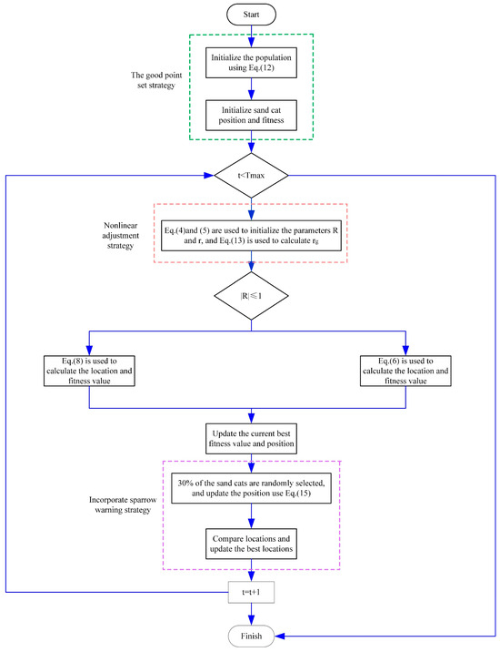
Figure 6.
MSCSO flow chart.
4. Experimental Results and Discussion
4.1. Experimental Design
In this experiment, the population size is set to 30, and the maximum number of iterations is 500. Each test function was independently calculated 30 times to obtain more accurate experimental results. The evaluation criteria are the data results’ mean value and standard deviation. The mean value represents the convergence accuracy of the algorithm, where a smaller value indicates higher accuracy. While the standard deviation represents the algorithm’s stability, with a more minor standard deviation indicating much better stability [28].
The CEC 2017 benchmark was adopted to evaluate the optimization algorithm’s global search ability and convergence performance. The CEC 2017 test functions incorporate complex and diverse optimization problems from real-life scenarios, mathematical models, and artificially constructed benchmark problems. Furthermore, the CEC 2017 test functions cover many optimization types, from simple local searches to complex global optimizations. As the dimensionality of the functions increases, the difficulty in solving them also escalates, posing more significant challenges to the performance of optimization algorithms. Therefore, this paper employs the 30-dimensional, 50-dimensional, and 100-dimensional functions from the CEC 2017 benchmark to verify the comprehensive performance of the optimization algorithm. Among the 29 essential test functions in CEC 2017, F1 and F2 are unimodal functions used to test the optimization capability and convergence speed. F3–F10 are simple multimodal functions with multiple local optima designed to evaluate the global search ability of the algorithm. F11–F20 are hybrid functions that combine unimodal and multimodal characteristics, requiring higher performance from the algorithm. F21–F30 are composition functions that reflect the comprehensive performance of the algorithm. However, F2 is not analyzed independently. Additionally, five intelligent optimization algorithms, namely DBO, POA, HHO, SABO, and SCSO, are utilized for comparative analysis with MSCSO. The specific parameters of these six intelligent algorithms are detailed in Table 2.
Table 2.
Algorithm parameter settings.
4.2. Results and Analysis
4.2.1. Analysis and Comparison of Experimental Results
As seen in Table 3, the MSCSO algorithm leads in terms of mean and standard deviation for the unimodal function F1. Among the simple multimodal functions F3–F10, MSCSO achieves the best mean and standard deviation for functions F3 and F4. The standard deviation of MSCSO for functions F7 and F10 is slightly higher than that of DBO and POA but lower than the original algorithm. It maintains a leading position for the remaining functions. In the simple multimodal functions, the average performance of MSCSO is average, ranking fifth and fourth in F5 and F6 and third in F7, F8, F9, and F10. For the mixed functions F11–F20, the MSCSO algorithm outperforms the other five in standard deviation for F11, F12, F13, F15, F16, and F19. The standard deviation of MSCSO for F14, F17, F18, and F120 is slightly higher than POA but better than the original algorithm. The average values rank fourth in F17 and second in F18. Among the composite functions F21–F30, MSCSO achieves the optimal mean and standard deviation for F23, F25, F27, F28, and F30. Although the mean value of MSCSO ranks fifth in F21, sixth in F22, second in F24, last in F26, and third in F29, its standard deviation remains leading among all composite functions.
Table 3.
CEC2017 30D test results.
As seen in Table A1, in the 50-dimensional experiments, the MSCSO algorithm outperforms the other five algorithms regarding mean and standard deviation for the unimodal function F1. Among the multimodal functions F3–F10, the evaluation metrics reach the optimal values for F4. The standard deviation is slightly higher than the DBO algorithm for F7 but performs excellently for the remaining functions. The average values for F5–F10 remain average. In the mixed functions F11–F20, the MSCSO algorithm demonstrates strong optimization performance. MSCSO ranks first in average values and standard deviations for F11–16 and F18–19. The standard deviation of MSCSO is only higher than POA for F20 but lower than the original algorithm. The average values rank average only for F17 and F20. In the composite functions F21-F30, the MSCSO algorithm’s standard deviation also performs outstandingly, consistently ranking first. The average values rank average for F21, F22, F24, and F26, but MSCSO can always find the solution fastest for the remaining functions.
As seen in Table A2, in the 100-dimensional experiments, the MSCSO algorithm exhibits excellent performance in handling complex problems. For the unimodal function F1, the evaluation metrics maintain the optimal state. Among the multimodal functions F3–F10, the optimization performance of the MSCSO algorithm is similar to that in the 50-dimensional experiments. In the mixed functions F11–F20, the average value of the MSCSO algorithm ranks only fourth in F17 and F20, and the standard deviation is higher than POA only in F20. The average and standard deviation exhibits the best performance for the remaining functions. In the composite functions F21–F30, the average value of the MSCSO algorithm ranks poorly only in F21 and F26, but the evaluation metrics maintain a leading position for the remaining functions.
In summary, the MSCSO algorithm performs averagely in handling simple multimodal problems. Still, it exhibits excellent performance in dealing with unimodal, mixed, and composite function problems, especially when handling complex composite and high-dimensional functions.
4.2.2. Convergence Plot Analysis Discussion
In this paper, convergence curves of six intelligent optimization algorithms on the CEC2017 benchmark in 30-dimensional, 50-dimensional, and 100-dimensional spaces are introduced to demonstrate the performance of optimization algorithms.
As seen in Figure A1, it can be observed that DBO and POA surpass the MSCSO algorithm in the later iterations of F6 and F14. However, its performance is significantly improved compared to the SCSO algorithm. In F3 and F22, the convergence performance of the algorithm is not evident in the early to mid-iterations. However, it accelerates in the later iterations, surpassing the other five algorithms and ranking first; it fully demonstrates that the algorithm’s integration of an early warning mechanism accelerates its convergence. In functions such as F1, F4, F5, F8, F9, F10, F12, F13, F19–F23, F26, F28, and F30, MSCSO exhibits faster convergence speeds. This acceleration in convergence speed indicates that MSCSO leverages the good point set strategy and nonlinear adjustment strategy to enhance its global search capabilities, enabling the algorithm to locate optimal solutions more rapidly and improve its convergence performance.
As seen in Figure A2, the MSCSO algorithm is only surpassed by DBO in F7 and needs to find the optimal solution. Among the other algorithms, it exhibits strong convergence and optimization performance. Compared to the original algorithm, it accelerates the convergence of the algorithm.
As seen in Figure A3, the MSCSO algorithm fails to find the optimal solution only in F20, but it can quickly find the optimal solution in most functions. Moreover, it can conduct a broader global search in the early iterations and escape from local optima in the later iterations, demonstrating that the MSCSO algorithm has certain advantages in handling complex and high-dimensional functions.
In summary, while the MSCSO algorithm exhibits some improvement in addressing the premature convergence and stagnation issues in the 30-dimensional experimental convergence curve, this improvement is not particularly evident in the 30-dimensional experiments. However, as the dimensionality increased, the algorithm’s convergence performance saw significant improvement, demonstrating that the MSCSO algorithm has certain advantages in handling complex and high-dimensional problems and can escape from local optima.
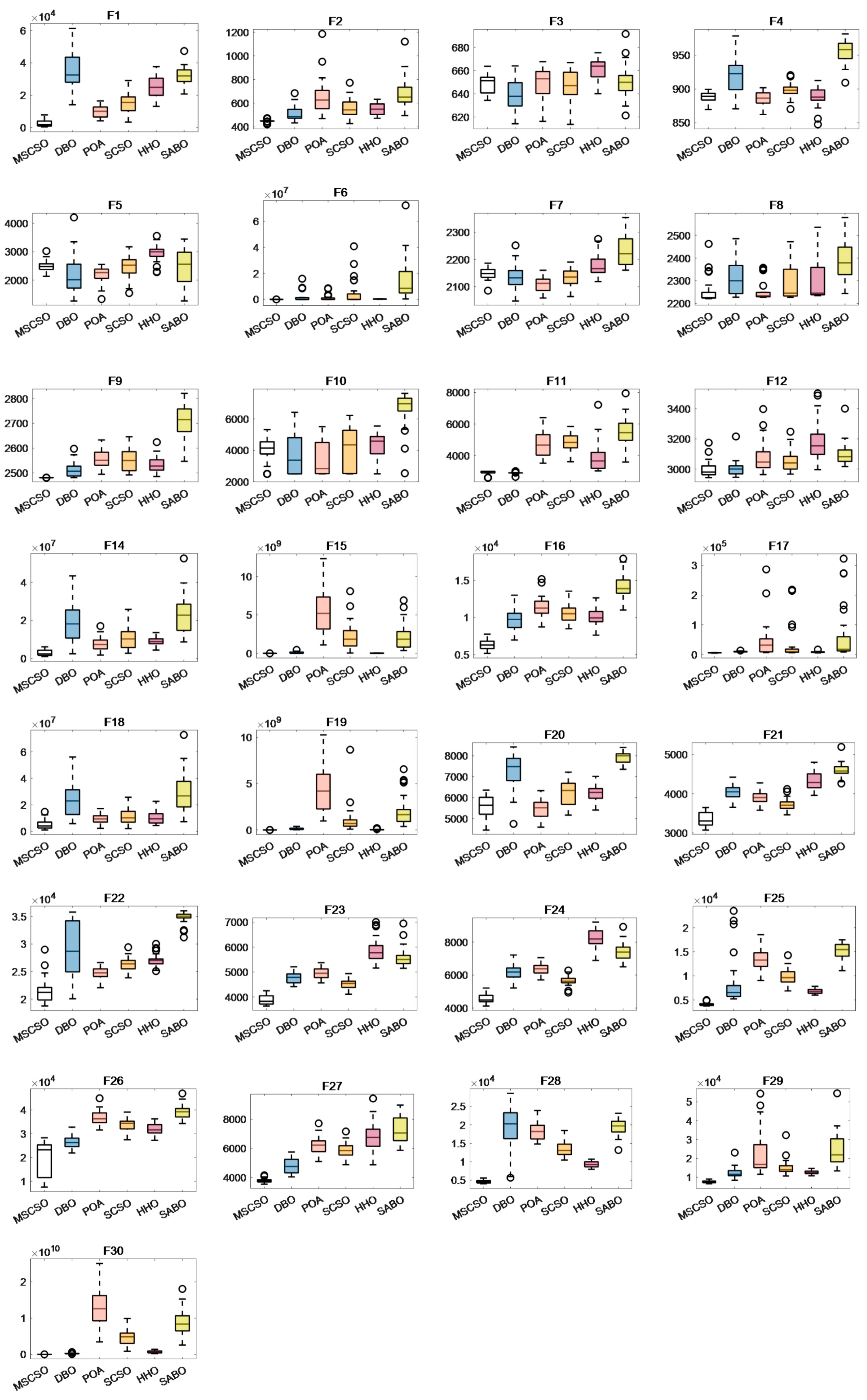
4.2.3. Boxplots Analysis
This paper utilizes boxplots to compare MSCSO with five other algorithms, making the optimization performance of MSCSO more visually intuitive. The median represents the average of the sample results after 30 independent runs of the algorithm. The upper and lower quartiles indicate the degree of fluctuation in the sample data to some extent. Outliers suggest instability in the data. Figure A4, Figure A5 and Figure A6 show the example data results of the six intelligent algorithms in 30-dimensional, 50-dimensional, and 100-dimensional test functions.
In Figure A4, MSCSO exhibits the lowest average value on most functions, verifying its powerful optimization capability. For test functions F6-F9, F16-F17, F20, F24, F26, and F29, the upper and lower quartiles of MSCSO’s boxplots are evenly distributed, indicating low data dispersion. Although there are outliers in some functions, the overall performance remains stable.
In Figure A5 and Figure A6, the box plots of MSCSO in 50-dimensional and 100-dimensional spaces show significant improvements in their upper and lower quartile distributions compared to the 30-dimensional boxplots. The distribution range becomes shorter and more uniform, indicating that as the dimension increases, the dispersion of the algorithm decreases. Additionally, as the dimension increases, the number of functions with the lowest average value for MSCSO also rises, demonstrating that MSCSO is more reliable than the other five algorithms.
4.3. Non-Parametric Test
4.3.1. Wilcoxon Rank-Sum Test
This paper introduces the Wilcoxon rank-sum test to verify whether there are significant differences in performance between MSCSO and the other five algorithms. Each algorithm was independently tested 30 times in the experiment. The results are used to calculate the p-values. The null hypothesis is rejected when the p-value is less than 0.05, indicating a significant performance difference between the two algorithms. When the p-value is more significant than 0.05, it suggests that the search results of the two algorithms are statistically significant [29].
From Table 4, it can be observed that 5.5% of the algorithms are comparable to the MSCSO algorithm. In functions F6 and F7, MSCSO’s performance is statistically significant compared to DBO. In functions F17, F18, and F22, MSCSO’s performance is comparable to POA. In functions F10 and F20, the p-values for SCSO are more significant than 0.05, indicating statistical significance. Additionally, 5.5% of the algorithms are comparable to the MSCSO algorithm.
Table 4.
Thirty-dimensional Wilcoxon rank-sum test of CEC2017 test function.
Table A3 indicates that only 2% of the algorithms have comparable performance to MSCSO, while 98% show significant differences from MSCSO. Specifically, in function F7, MSCSO’s performance is comparable to DBO. In functions F3 and F20, the p-values for POA are greater than 0.05, suggesting statistical significance.
In Table A4, 98.6% of the data results are less than 0.05, suggesting that MSCSO exhibits significant differences from the other five algorithms.
In summary, as the dimensionality of the test functions continues to increase, the significance of the differences between MSCSO and DBO, POA, SCSO, HHO, SABO, and SCSO becomes increasingly pronounced.
4.3.2. Friedman Test
In this paper, the Friedman Test is used to provide an overall ranking of the algorithm experimental results. The Friedman Test aids in comprehensively evaluating the overall performance of different algorithms. In this ranking, a smaller serial number for an algorithm indicates better performance. Figure 7 displays the average Friedman ranking of six intelligent optimization algorithms: DBO, POA, HHO, SABO, SCSO, and MSCSO. As evident from the figure, MSCSO consistently ranks first in the average ranking across the 30-dimensional, 50-dimensional, and 100-dimensional test functions of CEC2017, validating the effectiveness of the improved algorithm and demonstrating the excellent comprehensive performance of MSCSO.
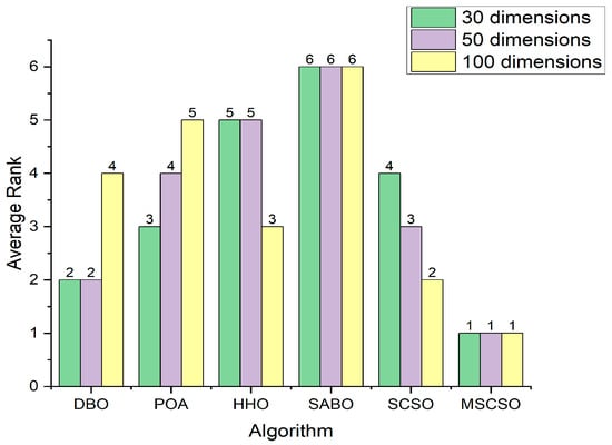
Figure 7.
Friedman average rank.
5. Engineering Applications
In this section, two specific engineering examples, the reducer design problem, and the welded beam design problem, are used to verify the performance of the MSCSO algorithm [30].
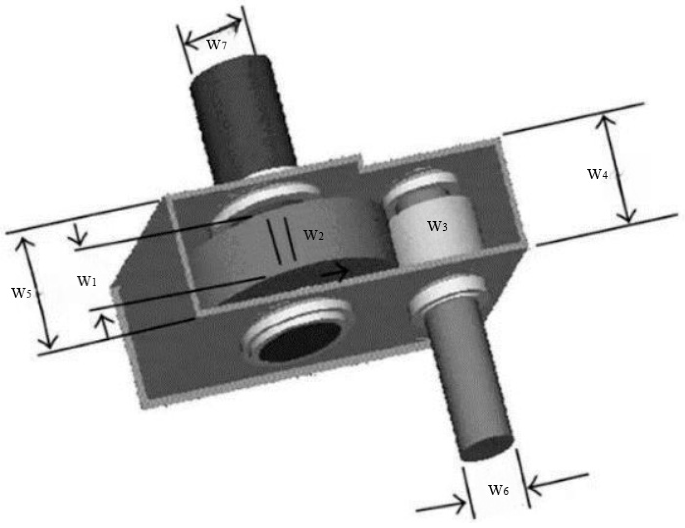
5.1. Reducer Design Problems
The reducer design problem is a classic constraint engineering optimization problem, and its core goal is to minimize the weight of the reducer under the premise of satisfying a series of complex constraints. As can be seen from Figure 1, this problem involves seven structural parameters: face width (W1), tooth die (W2), number of pinion teeth (W3), length of the first shaft between bearings (W4), length of the second shaft between bearings (W5), diameter of the first shaft (W6) and diameter of the second shaft (W7). By optimizing the combination of the seven parameters, the weight of the reducer is minimized, as shown in Figure 8.

Figure 8.
Reducer design.
W1, W2, W3, W4, W5, W6, W7 are the seven variables of the reducer design problem, and their objective functions are set as Equation (16) indicates.
Restrictions:
The range of the variables is as follows:
MSCSO is compared with DBO, POA, HHO, SABO, and SCSO algorithms to verify the performance of MSCSO in the reducer design problem. From the data in Table 5, compared with the other five algorithms, the MSCSO algorithm is the closest to the optimal value of the reducer design problem, with a value of 1.6702, and the values of its seven variables are 3.5, 0.7, 17, 7.3, 7.71532, 3.35054 and 5.28665.
Table 5.
Application of six intelligent algorithms in reducer design.
As seen in Figure 9, MSCSO can quickly find the global optimal solution compared to other algorithms, demonstrating its applicability in the reducer design problem.
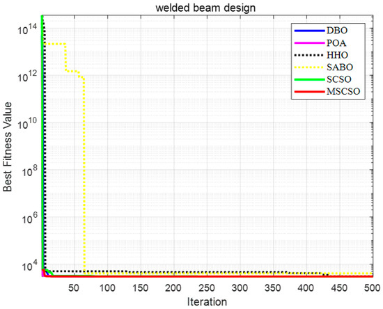
Figure 9.
Convergence curves of six algorithms in reducer design.
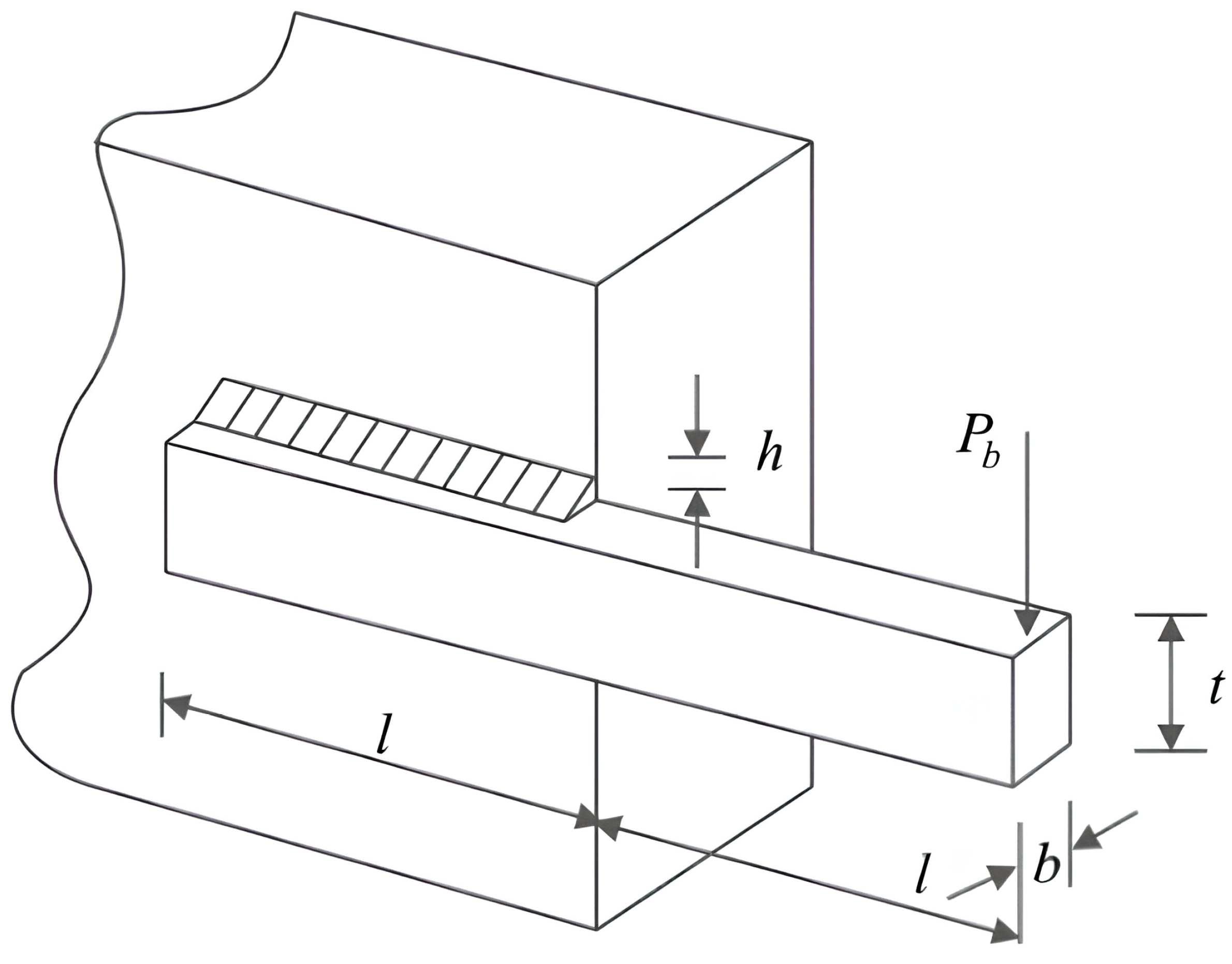
5.2. Welded Beam Design Problems
The welded beam design problem is a typical strongly constrained nonlinear programming problem, with its core objective being to reduce manufacturing costs by optimizing the design scheme. Figure 10 illustrates the structural parameters of the welded beam, where the optimal combination of joint thickness (h), tightening bar length (l), bar height (t), and bar thickness (b) is sought to minimize manufacturing costs, under the premise of satisfying various physical and engineering constraints.

Figure 10.
Welded beam design.
The parameters h, l, t, and b are represented by the variables w1, w2, w3, and w4, and their objective functions are set as Equation (17) indicates.
Restrictions:
The range of variables is as follows:
As seen from the data in Table 6, MSCSO shows superior performance compared with the five algorithms of DBO, POA, HHO, SABO, and SCSO in solving the welded beam design problem. Specifically, the optimal solutions of the four variables of the MSCSO algorithm are 0.19883, 3.3374, 9.1920, and 0.19883, respectively. The combination of the four variables accurately approximates the optimal solution, and its value is 2994.4245.
Table 6.
Application of six intelligent algorithms in welded beam design.
As seen in Figure 11, MSCSO can quickly locate the global optimal solution in the early stages of iteration for the welded beam design and converge effectively. The presence of multiple inflection points on the MSCSO curve indicates that MSCSO can escape from local optima.
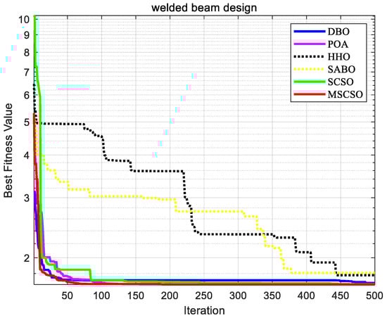
Figure 11.
Convergence curves of six algorithms in welded beam design.
6. Conclusions
This paper proposed a multi-strategy fusion algorithm named MSCSO to improve the optimization performance of SCSO. The effectiveness of MSCSO was verified through simulation experiments using 29 benchmark test functions from CEC 2017. Through detailed analysis and comparison of the experimental data, the following enhancements in MSCSO’s performance are observed.
- Precision and convergence speed in unimodal functions: MSCSO demonstrated significantly higher precision and faster convergence speed in unimodal functions than other algorithms; it indicated MSCSO’s superiority in efficiently navigating and exploiting simple search landscapes.
- Robust optimization performance in hybrid and composition functions: MSCSO exhibited formidable optimization capabilities in hybrid and composition functions. It maintained a leading position in precision and convergence in most functions, underscoring its adaptability to diverse and complex optimization challenges. As the problem dimensionality increases, MSCSO’s performance became even more pronounced, demonstrating its prowess in tackling intricate and high-dimensional problems.
- Superiority confirmed by Wilcoxon rank-sum test: The Wilcoxon rank-sum test statistically validated that MSCSO outperforms other algorithms, providing robust evidence of its enhanced performance.
- Applicability in engineering problems: In practical engineering applications such as gearbox reducer and welded beam design problems, MSCSO produced solutions closer to the optimal solutions than five other algorithms. It highlighted MSCSO’s effectiveness in real-world scenarios and underscored its broad applicability in solving engineering optimization tasks.
Author Contributions
All authors contributed to the conception and design of the study. Material preparation, data collection and analysis were carried out by H.P. and X.Z. The first draft of the manuscript was written by H.P., X.Z., H.M., Y.L., J.Q. and Z.K. All authors have commented on previous versions of the manuscript. All authors have read and agreed to the published version of the manuscript.
Funding
This work is supported by the Xinjiang Agricultural Machinery R and D, Manufacturing, Promotion and Application Integration Project (Autonomous Region Agricultural and Rural Mechanization Development Center YTHSD2022-19-3).
Data Availability Statement
The data used in the current study are available from the corresponding author on reasonable request.
Acknowledgments
The authors would like to thank the Engineering Research Center for Production Mechanization of Oasis Special Economic Crop, Ministry of Education for providing experimental materials.
Conflicts of Interest
The authors declare no conflicts of interest.
Appendix A
Table A1.
CEC2017 50D test results.
Table A1.
CEC2017 50D test results.
| DBO | POA | HHO | SABO | SCSO | MSCSO | ||
|---|---|---|---|---|---|---|---|
| F1 | Mean | 3302398088 | 10390489898 | 1484653454 | 8799881201 | 8778375893 | 196284819 |
| Std | 3899252845 | 49823118066 | 5512734336 | 42119582938 | 30042244589 | 61728185.7 | |
| F3 | Mean | 66786.35118 | 22023.41482 | 18437.34617 | 16561.57008 | 13980.77039 | 17413.1313 |
| Std | 268106.3887 | 117684.1181 | 167032.023 | 182813.6126 | 133707.5058 | 99157.0174 | |
| F4 | Mean | 524.8249642 | 2726.350905 | 480.1093044 | 3027.911409 | 1656.421951 | 53.2610363 |
| Std | 1409.957618 | 7812.684022 | 1805.635567 | 8077.440603 | 4571.652584 | 567.295001 | |
| F5 | Mean | 84.95671361 | 40.22758238 | 31.12382383 | 43.52121811 | 36.853378 | 43.369063 |
| Std | 960.315895 | 926.2623231 | 922.5744492 | 1103.391257 | 948.8158352 | 838.558676 | |
| F6 | Mean | 11.32040522 | 6.237167532 | 4.065757496 | 12.3553266 | 7.190901281 | 7.57760074 |
| Std | 668.8507287 | 672.129517 | 679.9782754 | 686.2532994 | 677.4816775 | 656.270736 | |
| F7 | Mean | 135.3215707 | 90.41802472 | 69.8349611 | 79.64051781 | 110.3563116 | 131.381464 |
| Std | 1412.10116 | 1764.55676 | 1899.381916 | 1632.291613 | 1665.295017 | 1464.57607 | |
| F8 | Mean | 83.01299842 | 39.82495196 | 38.7444479 | 43.10136231 | 51.18661919 | 50.2141428 |
| Std | 1321.315603 | 1255.066828 | 1244.088564 | 1426.266704 | 1290.516019 | 1161.60697 | |
| F9 | Mean | 7710.747487 | 1529.036855 | 2603.718659 | 3922.344162 | 3210.250677 | 2219.92498 |
| Std | 25806.01922 | 18620.38525 | 32122.69238 | 31402.25016 | 21158.10829 | 12664.2894 | |
| F10 | Mean | 2272.307432 | 630.9933193 | 950.8373144 | 368.7032054 | 1119.804333 | 1573.49553 |
| Std | 11510.69442 | 9181.627844 | 10355.83564 | 15130.59108 | 10190.86836 | 8705.85798 | |
| F11 | Mean | 1322.890937 | 2470.236447 | 526.0597284 | 2745.167283 | 2255.918509 | 82.9280624 |
| Std | 4033.575553 | 6728.049967 | 2988.033843 | 11606.62784 | 7861.105679 | 1379.4339 | |
| F12 | Mean | 538853153.4 | 7237740245 | 567912624.7 | 7960953201 | 2208829317 | 6744695.91 |
| Std | 830186029.6 | 14648371591 | 954810132.7 | 13876884946 | 3833950125 | 10351644.2 | |
| F13 | Mean | 114150217.4 | 4494947129 | 41254837.95 | 2425906523 | 1903746602 | 35670.1713 |
| Std | 92502949.45 | 4707351617 | 33200051.09 | 2580833263 | 1474877114 | 56441.5596 | |
| F14 | Mean | 3974759.282 | 607675.3837 | 3910591.193 | 5374681.808 | 2703986.653 | 146418.047 |
| Std | 3918959.364 | 649914.5906 | 4748048.359 | 6304012.675 | 2681790.879 | 310747.588 | |
| F15 | Mean | 23480267.91 | 175874736.5 | 955411.5079 | 296542849.3 | 424171520.7 | 14866.0908 |
| Std | 9825049.542 | 88883732.08 | 1495111.31 | 238992978.7 | 189176839.5 | 28855.0623 | |
| F16 | Mean | 628.3633522 | 692.8244518 | 665.4755948 | 562.5161157 | 569.3277895 | 532.561722 |
| Std | 4989.421503 | 4372.086747 | 4990.462575 | 6001.400479 | 4672.412437 | 3592.24632 | |
| F17 | Mean | 429.73778 | 408.269056 | 485.9001181 | 365.0381958 | 479.430001 | 426.899651 |
| Std | 4413.380306 | 3774.015327 | 3828.298961 | 4618.758234 | 3919.009562 | 3492.97037 | |
| F18 | Mean | 14964943.25 | 4418438.238 | 6842181.004 | 28288404.34 | 24711295.34 | 1272072.92 |
| Std | 15796585.34 | 4262892.242 | 10795307.23 | 40890071.68 | 23837109.2 | 1564630.47 | |
| F19 | Mean | 13933122.64 | 362744484.7 | 3677685.849 | 50424696.53 | 222217039.8 | 14766.5931 |
| Std | 9116184.623 | 149962044.9 | 3069100.459 | 50048950.38 | 70718954.71 | 37005.8523 | |
| F20 | Mean | 410.2578286 | 213.5439526 | 308.4450941 | 168.3324002 | 294.2973357 | 345.601964 |
| Std | 3710.28514 | 3063.836687 | 3668.520885 | 4212.271348 | 3565.674877 | 3335.5459 | |
| F21 | Mean | 83.14094219 | 61.95986229 | 101.6349972 | 63.59623969 | 73.23544841 | 66.0088371 |
| Std | 2876.18541 | 2827.935196 | 2958.650285 | 2934.355452 | 2794.594213 | 2648.16974 | |
| F22 | Mean | 2015.922742 | 1074.838903 | 823.2283951 | 2343.895269 | 985.7160627 | 1602.4466 |
| Std | 12502.87764 | 11437.60931 | 12417.40035 | 16309.13028 | 12327.33491 | 10992.8653 | |
| F23 | Mean | 132.4932719 | 147.379751 | 206.4727144 | 180.1562827 | 123.2249366 | 114.317005 |
| Std | 3523.633457 | 3590.806985 | 3990.493109 | 3943.872193 | 3384.520633 | 3182.09634 | |
| F24 | Mean | 158.7447433 | 109.0159033 | 255.7003902 | 158.4743871 | 104.2052828 | 106.811743 |
| Std | 3695.170402 | 3733.672181 | 4419.94957 | 3913.251521 | 3537.007824 | 3320.05097 | |
| F25 | Mean | 1569.240404 | 1094.525409 | 162.705011 | 1287.475791 | 663.4378573 | 27.3972524 |
| Std | 3861.611951 | 6999.033404 | 3816.319194 | 7075.942069 | 5232.677992 | 3114.66829 | |
| F26 | Mean | 1118.232735 | 1865.600314 | 1342.11311 | 842.5372236 | 1614.13788 | 3234.80923 |
| Std | 11100.88082 | 12768.05974 | 11536.63164 | 13553.13631 | 11748.54079 | 5729.92126 | |
| F27 | Mean | 308.0431984 | 291.1735528 | 683.8444814 | 492.0369643 | 207.7881354 | 169.730378 |
| Std | 4010.032961 | 4339.722563 | 5155.284814 | 4642.827783 | 4274.549997 | 3611.67258 | |
| F28 | Mean | 2254.867558 | 755.4207857 | 441.8933227 | 825.6899025 | 570.2134973 | 87.1245666 |
| Std | 6131.061848 | 6815.875429 | 4758.024815 | 7617.282993 | 5661.331436 | 3377.80703 | |
| F29 | Mean | 1002.694976 | 621.4094541 | 1096.522217 | 1507.201481 | 822.3748579 | 485.91776 |
| Std | 6231.20715 | 7022.556572 | 7345.788008 | 9940.701573 | 6901.555629 | 4970.4202 | |
| F30 | Mean | 47489390.7 | 242380028.8 | 51564123.09 | 603825274.3 | 112349961.3 | 1336896.06 |
| Std | 60009001.81 | 346537086.2 | 128720404.5 | 734334649 | 220873074 | 2431763.66 |
Table A2.
CEC2017 100D test results.
Table A2.
CEC2017 100D test results.
| DBO | POA | HHO | SABO | SCSO | MSCSO | ||
|---|---|---|---|---|---|---|---|
| F1 | Mean | 64439785350 | 14679470611 | 7123064242 | 12786225157 | 13574141598 | 6191835519 |
| Std | 88946907692 | 1.44787 × 10¹¹ | 48058863472 | 1.56287 × 10¹¹ | 1.06645 × 10¹¹ | 1.8053 × 10¹⁰ | |
| F3 | Mean | 327312.9072 | 31671.50162 | 122549.3883 | 14531.95724 | 17342.92473 | 30730.8664 |
| Std | 730924.6607 | 305881.7838 | 372984.6991 | 348932.4274 | 320105.4844 | 298781.525 | |
| F4 | Mean | 15071.01887 | 6198.775365 | 1998.389853 | 6240.446945 | 4582.407811 | 1073.78027 |
| Std | 16471.56686 | 25602.81592 | 9838.835433 | 31928.30398 | 15787.59256 | 1733.29016 | |
| F5 | Mean | 255.9942286 | 64.41293008 | 46.42333274 | 113.6177764 | 60.19254203 | 50.4321657 |
| Std | 1737.151357 | 1606.074738 | 1673.752052 | 1930.352906 | 1632.976958 | 1371.77767 | |
| F6 | Mean | 13.17570887 | 3.748854711 | 3.847419004 | 5.791203439 | 4.652130833 | 3.18444647 |
| Std | 682.8830424 | 681.3642251 | 690.6116046 | 705.539359 | 686.9988035 | 664.088596 | |
| F7 | Mean | 230.5354516 | 80.11767378 | 131.0653554 | 183.3490029 | 204.1486638 | 207.995493 |
| Std | 2978.277946 | 3470.650798 | 3776.686954 | 3405.051846 | 3424.583953 | 2882.10396 | |
| F8 | Mean | 203.1690199 | 69.75688334 | 67.34965118 | 97.75941497 | 76.22128493 | 120.07328 |
| Std | 2215.08076 | 2086.033586 | 2132.86936 | 2360.188236 | 2085.977332 | 1762.19817 | |
| F9 | Mean | 6031.929811 | 3543.233864 | 4754.054793 | 4463.180529 | 5964.901628 | 1649.51376 |
| Std | 78882.20914 | 41704.00481 | 68787.89439 | 78575.29059 | 44974.51707 | 26104.6671 | |
| F10 | Mean | 5235.205338 | 1140.992805 | 1997.673166 | 731.0527176 | 1614.762398 | 2533.84918 |
| Std | 27335.04082 | 21101.19419 | 24224.20078 | 32359.4073 | 22747.04663 | 17293.8057 | |
| F11 | Mean | 68644.9515 | 18627.26318 | 38471.07732 | 42124.32695 | 23270.27405 | 6659.60843 |
| Std | 223448.5264 | 88617.44402 | 144597.4059 | 205655.4621 | 94315.73489 | 28493.7276 | |
| F12 | Mean | 2268580864 | 16365928649 | 2676065431 | 18164454902 | 13817550434 | 441613219 |
| Std | 7277633037 | 68930637601 | 11619528549 | 54872552598 | 36736964033 | 255071073 | |
| F13 | Mean | 192201584.9 | 5459325140 | 196797367.5 | 4378193430 | 3222776818 | 30025.803 |
| Std | 264566938.2 | 15150913501 | 340976541.6 | 8883083561 | 5668646842 | 65185.9529 | |
| F14 | Mean | 11153472.54 | 3516377.125 | 2237802.183 | 9886433.727 | 5827627.548 | 1513169.62 |
| Std | 18865348.02 | 7659394.616 | 9054348.956 | 23213173.86 | 10840847.18 | 2950801.58 | |
| F15 | Mean | 109477038 | 2800000225 | 10706452.68 | 1617740396 | 1859453612 | 24423.7711 |
| Std | 91000114.11 | 5414412363 | 18070615.52 | 2194201582 | 2129450783 | 44422.7137 | |
| F16 | Mean | 1437.527393 | 1401.778021 | 1127.143 | 1675.072261 | 1129.010461 | 687.019308 |
| Std | 9830.457777 | 11418.37002 | 10048.44809 | 14272.76565 | 10546.5916 | 6353.67028 | |
| F17 | Mean | 1446.023266 | 60266.75664 | 2015.379609 | 87948.15107 | 55169.84024 | 647.352039 |
| Std | 9522.423148 | 44338.51265 | 8111.732752 | 58510.76338 | 30618.69714 | 5891.41214 | |
| F18 | Mean | 13836695.43 | 3976344.651 | 4860168.729 | 14620039.89 | 5884800.631 | 3282615.36 |
| Std | 24279018.43 | 9314116.26 | 10333720.11 | 29683396.12 | 11376427.43 | 4933958.16 | |
| F19 | Mean | 104306523.7 | 2451264977 | 36239372.08 | 1655661585 | 1570265191 | 91064.6918 |
| Std | 139026655.4 | 4336804118 | 40238023.7 | 2111376240 | 1058246800 | 36491.2231 | |
| F20 | Mean | 873.1403828 | 485.1281919 | 391.7970499 | 288.1319208 | 574.8553324 | 492.113677 |
| Std | 7283.694865 | 5452.846214 | 6232.521204 | 7911.433915 | 6246.751869 | 5591.37673 | |
| F21 | Mean | 194.6733628 | 151.272736 | 240.8060467 | 174.772987 | 158.0561619 | 150.778371 |
| Std | 4034.475166 | 3900.882946 | 4336.474513 | 4609.40168 | 3732.258314 | 3344.92746 | |
| F22 | Mean | 4982.55286 | 1240.221994 | 1250.068268 | 1073.874386 | 1304.752149 | 2262.16708 |
| Std | 29603.2738 | 24731.09808 | 27107.14681 | 34789.05817 | 26263.40432 | 21557.4056 | |
| F23 | Mean | 228.9527889 | 228.6376536 | 463.797077 | 382.3292313 | 187.8860342 | 170.356698 |
| Std | 4774.38515 | 4964.923155 | 5861.948017 | 5563.140243 | 4534.221736 | 3861.13035 | |
| F24 | Mean | 434.7971439 | 293.7675921 | 601.9109496 | 544.0433336 | 292.4855238 | 254.89335 |
| Std | 6174.067484 | 6366.875405 | 8242.826952 | 7426.1978 | 5655.794757 | 4576.10926 | |
| F25 | Mean | 4971.625162 | 2146.970151 | 469.6290082 | 1718.771909 | 1580.137642 | 280.365032 |
| Std | 8528.152533 | 13375.00475 | 6799.205617 | 15072.28933 | 9867.156162 | 4069.11079 | |
| F26 | Mean | 2716.297116 | 2893.558169 | 2197.696998 | 2627.738246 | 2775.087158 | 7306.39958 |
| Std | 26555.3795 | 36793.64805 | 31943.81382 | 39199.66094 | 33818.41939 | 19838.3825 | |
| F27 | Mean | 517.8607132 | 624.4369159 | 1066.926374 | 907.8012227 | 519.8501265 | 142.25572 |
| Std | 4796.677845 | 6170.744599 | 6821.516679 | 7226.379513 | 5855.303843 | 3782.70941 | |
| F28 | Mean | 6867.524167 | 2361.314563 | 803.4499535 | 2055.769571 | 1887.503296 | 420.03276 |
| Std | 18557.442 | 18477.30251 | 9319.445458 | 19527.98794 | 13378.17802 | 4602.70205 | |
| F29 | Mean | 2818.558281 | 10708.19759 | 1042.989965 | 8864.106404 | 3914.703263 | 617.239425 |
| Std | 12278.1268 | 22161.34028 | 12642.23408 | 24025.07565 | 15093.16939 | 7535.46986 | |
| F30 | Mean | 109769797.4 | 4948234972 | 294385332.6 | 3570975523 | 2380766605 | 930694.966 |
| Std | 241833483.5 | 13085971393 | 669153209.3 | 8978885602 | 4603212747 | 981372.554 |
Table A3.
Fifty-dimensional Wilcoxon rank-sum test of CEC2017 test function.
Table A3.
Fifty-dimensional Wilcoxon rank-sum test of CEC2017 test function.
| DBO | POA | HHO | SABO | SCSO | |
|---|---|---|---|---|---|
| F1 | 3.6 × 10⁻¹¹ < 0.05 | 3.0 × 10⁻¹¹ < 0.05 | 3.0 × 10⁻¹¹ < 0.05 | 3.0 × 10⁻¹¹ < 0.05 | 3.0 × 10⁻¹¹ < 0.05 |
| F3 | 8.9 × 10⁻¹¹ < 0.05 | 3.2 × 10−01 > 0.05 | 1.1 × 10−05 < 0.05 | 2.8 × 10−06 < 0.05 | 3.2 × 10−02 < 0.05 |
| F4 | 3.0 × 10⁻¹¹ < 0.05 | 3.0 × 10⁻¹¹ < 0.05 | 3.0 × 10⁻¹¹ < 0.05 | 3.0 × 10⁻¹¹ < 0.05 | 3.0 × 10⁻¹¹ < 0.05 |
| F5 | 2.2 × 10−09 < 0.05 | 3.0 × 10⁻¹¹ < 0.05 | 3.0 × 10⁻¹¹ < 0.05 | 3.0 × 10⁻¹¹ < 0.05 | 3.0 × 10⁻¹¹ < 0.05 |
| F6 | 7.5 × 10−07 < 0.05 | 3.0 × 10⁻¹¹ < 0.05 | 3.0 × 10⁻¹¹ < 0.05 | 3.0 × 10⁻¹¹ < 0.05 | 3.0 × 10⁻¹¹ < 0.05 |
| F7 | 6.5 × 10−01 > 0.05 | 3.0 × 10⁻¹¹ < 0.05 | 3.0 × 10⁻¹¹ < 0.05 | 4.6 × 10⁻¹⁰ < 0.05 | 1.4 × 10−08 < 0.05 |
| F8 | 9.7 × 10⁻¹⁰ < 0.05 | 3.0 × 10⁻¹¹ < 0.05 | 3.0 × 10⁻¹¹ < 0.05 | 3.0 × 10⁻¹¹ < 0.05 | 3.0 × 10⁻¹¹ < 0.05 |
| F9 | 3.0 × 10⁻¹¹ < 0.05 | 3.0 × 10⁻¹¹ < 0.05 | 3.0 × 10⁻¹¹ < 0.05 | 3.0 × 10⁻¹¹ < 0.05 | 3.0 × 10⁻¹¹ < 0.05 |
| F10 | 7.3 × 10⁻¹⁰ < 0.05 | 5.1 × 10−07 < 0.05 | 4.0 × 10⁻¹¹ < 0.05 | 3.0 × 10⁻¹¹ < 0.05 | 1.5 × 10−09 < 0.05 |
| F11 | 3.0 × 10⁻¹¹ < 0.05 | 3.0 × 10⁻¹¹ < 0.05 | 3.0 × 10⁻¹¹ < 0.05 | 3.0 × 10⁻¹¹ < 0.05 | 3.0 × 10⁻¹¹ < 0.05 |
| F12 | 2.3 × 10⁻¹⁰ < 0.05 | 3.0 × 10⁻¹¹ < 0.05 | 6.0 × 10⁻¹¹ < 0.05 | 3.0 × 10⁻¹¹ < 0.05 | 3.0 × 10⁻¹¹ < 0.05 |
| F13 | 3.0 × 10⁻¹¹ < 0.05 | 3.0 × 10⁻¹¹ < 0.05 | 3.0 × 10⁻¹¹ < 0.05 | 3.0 × 10⁻¹¹ < 0.05 | 3.0 × 10⁻¹¹ < 0.05 |
| F14 | 4.6 × 10−08 < 0.05 | 1.6 × 10−05 < 0.05 | 1.1 × 10−09 < 0.05 | 3.0 × 10⁻¹¹ < 0.05 | 7.3 × 10⁻¹⁰ < 0.05 |
| F15 | 3.0 × 10⁻¹¹ < 0.05 | 3.0 × 10⁻¹¹ < 0.05 | 3.0 × 10⁻¹¹ < 0.05 | 3.0 × 10⁻¹¹ < 0.05 | 3.0 × 10⁻¹¹ < 0.05 |
| F16 | 8.9 × 10⁻¹¹ < 0.05 | 3.3 × 10⁻¹¹ < 0.05 | 3.0 × 10⁻¹¹ < 0.05 | 3.0 × 10⁻¹¹ < 0.05 | 3.0 × 10⁻¹¹ < 0.05 |
| F17 | 3.0 × 10⁻¹¹ < 0.05 | 3.0 × 10⁻¹¹ < 0.05 | 3.3 × 10⁻¹¹ < 0.05 | 3.0 × 10⁻¹¹ < 0.05 | 1.2 × 10⁻¹⁰ < 0.05 |
| F18 | 1.8 × 10−09 < 0.05 | 1.8 × 10−06 < 0.05 | 7.5 × 10−07 < 0.05 | 3.0 × 10⁻¹¹ < 0.05 | 1.4 × 10−07 < 0.05 |
| F19 | 3.0 × 10⁻¹¹ < 0.05 | 3.0 × 10⁻¹¹ < 0.05 | 3.0 × 10⁻¹¹ < 0.05 | 3.0 × 10⁻¹¹ < 0.05 | 3.0 × 10⁻¹¹ < 0.05 |
| F20 | 7.7 × 10−09 < 0.05 | 3.4 × 10−01 > 0.05 | 5.3 × 10−03 < 0.05 | 3.0 × 10⁻¹¹ < 0.05 | 5.5 × 10−03 < 0.05 |
| F21 | 4.5 × 10⁻¹¹ < 0.05 | 3.0 × 10⁻¹¹ < 0.05 | 3.0 × 10⁻¹¹ < 0.05 | 3.0 × 10⁻¹¹ < 0.05 | 1.6 × 10⁻¹⁰ < 0.05 |
| F22 | 2.0 × 10−08 < 0.05 | 5.1 × 10−07 < 0.05 | 1.7 × 10⁻¹⁰ < 0.05 | 3.0 × 10⁻¹¹ < 0.05 | 4.6 × 10−08 < 0.05 |
| F23 | 3.0 × 10⁻¹¹ < 0.05 | 3.0 × 10⁻¹¹ < 0.05 | 3.0 × 10⁻¹¹ < 0.05 | 3.0 × 10⁻¹¹ < 0.05 | 1.2 × 10⁻¹⁰ < 0.05 |
| F24 | 3.0 × 10⁻¹¹ < 0.05 | 3.0 × 10⁻¹¹ < 0.05 | 3.0 × 10⁻¹¹ < 0.05 | 3.0 × 10⁻¹¹ < 0.05 | 4.5 × 10⁻¹¹ < 0.05 |
| F25 | 3.0 × 10⁻¹¹ < 0.05 | 3.0 × 10⁻¹¹ < 0.05 | 3.0 × 10⁻¹¹ < 0.05 | 3.0 × 10⁻¹¹ < 0.05 | 3.0 × 10⁻¹¹ < 0.05 |
| F26 | 6.9 × 10−03 < 0.05 | 3.0 × 10⁻¹¹ < 0.05 | 3.6 × 10⁻¹¹ < 0.05 | 3.0 × 10⁻¹¹ < 0.05 | 1.4 × 10⁻¹⁰ < 0.05 |
| F27 | 1.9 × 10⁻¹⁰ < 0.05 | 3.0 × 10⁻¹¹ < 0.05 | 3.0 × 10⁻¹¹ < 0.05 | 3.0 × 10⁻¹¹ < 0.05 | 3.0 × 10⁻¹¹ < 0.05 |
| F28 | 3.0 × 10⁻¹¹ < 0.05 | 3.0 × 10⁻¹¹ < 0.05 | 3.0 × 10⁻¹¹ < 0.05 | 3.0 × 10⁻¹¹ < 0.05 | 3.0 × 10⁻¹¹ < 0.05 |
| F29 | 3.6 × 10⁻¹¹ < 0.05 | 3.0 × 10⁻¹¹ < 0.05 | 3.0 × 10⁻¹¹ < 0.05 | 3.0 × 10⁻¹¹ < 0.05 | 3.0 × 10⁻¹¹ < 0.05 |
| F30 | 3.0 × 10⁻¹¹ < 0.05 | 3.0 × 10⁻¹¹ < 0.05 | 3.0 × 10⁻¹¹ < 0.05 | 3.0 × 10⁻¹¹ < 0.05 | 3.0 × 10⁻¹¹ < 0.05 |
Table A4.
One-hundred-dimensional Wilcoxon rank-sum test of CEC2017 test function.
Table A4.
One-hundred-dimensional Wilcoxon rank-sum test of CEC2017 test function.
| DBO | POA | HHO | SABO | SCSO | |
|---|---|---|---|---|---|
| F1 | 1.8 × 10−09 < 0.05 | 1.8 × 10−06 < 0.05 | 7.5 × 10−07 < 0.05 | 3.0 × 10⁻¹¹ < 0.05 | 1.4 × 10−07 < 0.05 |
| F3 | 8.9 × 10⁻¹¹ < 0.05 | 4.9 × 10−01 > 0.05 | 1.1 × 10−05 < 0.05 | 2.8 × 10−06 < 0.05 | 3.2 × 10−02 < 0.05 |
| F4 | 3.0 × 10⁻¹¹ < 0.05 | 3.0 × 10⁻¹¹ < 0.05 | 3.0 × 10⁻¹¹ < 0.05 | 3.0 × 10⁻¹¹ < 0.05 | 3.0 × 10⁻¹¹ < 0.05 |
| F5 | 2.2 × 10−09 < 0.05 | 3.0 × 10⁻¹¹ < 0.05 | 3.0 × 10⁻¹¹ < 0.05 | 3.0 × 10⁻¹¹ < 0.05 | 3.0 × 10⁻¹¹ < 0.05 |
| F6 | 7.5 × 10−07 < 0.05 | 3.0 × 10⁻¹¹ < 0.05 | 3.0 × 10⁻¹¹ < 0.05 | 3.0 × 10⁻¹¹ < 0.05 | 3.0 × 10⁻¹¹ < 0.05 |
| F7 | 7.5 × 10−07 < 0.05 | 3.0 × 10⁻¹¹ < 0.05 | 3.0 × 10⁻¹¹ < 0.05 | 4.6 × 10⁻¹⁰ < 0.05 | 1.4 × 10−08 < 0.05 |
| F8 | 9.7 × 10⁻¹⁰ < 0.05 | 3.0 × 10⁻¹¹ < 0.05 | 3.0 × 10⁻¹¹ < 0.05 | 3.0 × 10⁻¹¹ < 0.05 | 3.0 × 10⁻¹¹ < 0.05 |
| F9 | 3.0 × 10⁻¹¹ < 0.05 | 3.0 × 10⁻¹¹ < 0.05 | 3.0 × 10⁻¹¹ < 0.05 | 3.0 × 10⁻¹¹ < 0.05 | 3.0 × 10⁻¹¹ < 0.05 |
| F10 | 7.3 × 10⁻¹⁰ < 0.05 | 5.1 × 10−07 < 0.05 | 3.0 × 10⁻¹¹ < 0.05 | 3.0 × 10⁻¹¹ < 0.05 | 1.5 × 10−09 < 0.05 |
| F11 | 3.0 × 10⁻¹¹ < 0.05 | 3.0 × 10⁻¹¹ < 0.05 | 3.0 × 10⁻¹¹ < 0.05 | 3.0 × 10⁻¹¹ < 0.05 | 3.0 × 10⁻¹¹ < 0.05 |
| F12 | 3.0 × 10⁻¹¹ < 0.05 | 3.0 × 10⁻¹¹ < 0.05 | 3.0 × 10⁻¹¹ < 0.05 | 3.0 × 10⁻¹¹ < 0.05 | 3.0 × 10⁻¹¹ < 0.05 |
| F13 | 2.3 × 10⁻¹⁰ < 0.05 | 3.0 × 10⁻¹¹ < 0.05 | 3.0 × 10⁻¹¹ < 0.05 | 3.0 × 10⁻¹¹ < 0.05 | 3.0 × 10⁻¹¹ < 0.05 |
| F14 | 3.0 × 10⁻¹¹ < 0.05 | 3.0 × 10⁻¹¹ < 0.05 | 3.0 × 10⁻¹¹ < 0.05 | 3.0 × 10⁻¹¹ < 0.05 | 3.0 × 10⁻¹¹ < 0.05 |
| F15 | 3.0 × 10⁻¹¹ < 0.05 | 3.0 × 10⁻¹¹ < 0.05 | 3.0 × 10⁻¹¹ < 0.05 | 3.0 × 10⁻¹¹ < 0.05 | 3.0 × 10⁻¹¹ < 0.05 |
| F16 | 8.9 × 10⁻¹¹ < 0.05 | 3.3 × 10⁻¹¹ < 0.05 | 3.0 × 10⁻¹¹ < 0.05 | 3.0 × 10⁻¹¹ < 0.05 | 3.0 × 10⁻¹¹ < 0.05 |
| F17 | 3.0 × 10⁻¹¹ < 0.05 | 3.0 × 10⁻¹¹ < 0.05 | 3.0 × 10⁻¹¹ < 0.05 | 3.0 × 10⁻¹¹ < 0.05 | 1.2 × 10⁻¹⁰ < 0.05 |
| F18 | 1.8 × 10−09 < 0.05 | 1.8 × 10−06 < 0.05 | 7.5 × 10−07 < 0.05 | 3.0 × 10⁻¹¹ < 0.05 | 1.4 × 10−07 < 0.05 |
| F19 | 3.0 × 10⁻¹¹ < 0.05 | 3.0 × 10⁻¹¹ < 0.05 | 3.0 × 10⁻¹¹ < 0.05 | 3.0 × 10⁻¹¹ < 0.05 | 3.0 × 10⁻¹¹ < 0.05 |
| F20 | 7.7 × 10−09 < 0.05 | 2.3 × 10−01 > 0.05 | 5.3 × 10−03 < 0.05 | 3.0 × 10⁻¹¹ < 0.05 | 5.5 × 10−03 < 0.05 |
| F21 | 4.5 × 10⁻¹¹ < 0.05 | 3.0 × 10⁻¹¹ < 0.05 | 3.0 × 10⁻¹¹ < 0.05 | 3.0 × 10⁻¹¹ < 0.05 | 1.6 × 10⁻¹⁰ < 0.05 |
| F22 | 2.0 × 10−08 < 0.05 | 5.1 × 10−07 < 0.05 | 3.0 × 10⁻¹¹ < 0.05 | 3.0 × 10⁻¹¹ < 0.05 | 4.6 × 10−08 < 0.05 |
| F23 | 3.0 × 10⁻¹¹ < 0.05 | 3.0 × 10⁻¹¹ < 0.05 | 3.0 × 10⁻¹¹ < 0.05 | 3.0 × 10⁻¹¹ < 0.05 | 1.2 × 10⁻¹⁰ < 0.05 |
| F24 | 3.0 × 10⁻¹¹ < 0.05 | 3.0 × 10⁻¹¹ < 0.05 | 3.0 × 10⁻¹¹ < 0.05 | 3.0 × 10⁻¹¹ < 0.05 | 3.0 × 10⁻¹¹ < 0.05 |
| F25 | 3.0 × 10⁻¹¹ < 0.05 | 3.0 × 10⁻¹¹ < 0.05 | 3.0 × 10⁻¹¹ < 0.05 | 3.0 × 10⁻¹¹ < 0.05 | 3.0 × 10⁻¹¹ < 0.05 |
| F26 | 6.9 × 10−03 < 0.05 | 3.0 × 10⁻¹¹ < 0.05 | 3.0 × 10⁻¹¹ < 0.05 | 3.0 × 10⁻¹¹ < 0.05 | 1.4 × 10⁻¹⁰ < 0.05 |
| F27 | 1.9 × 10⁻¹⁰ < 0.05 | 3.0 × 10⁻¹¹ < 0.05 | 3.0 × 10⁻¹¹ < 0.05 | 3.0 × 10⁻¹¹ < 0.05 | 3.0 × 10⁻¹¹ < 0.05 |
| F28 | 3.0 × 10⁻¹¹ < 0.05 | 3.0 × 10⁻¹¹ < 0.05 | 3.0 × 10⁻¹¹ < 0.05 | 3.0 × 10⁻¹¹ < 0.05 | 3.0 × 10⁻¹¹ < 0.05 |
| F29 | 7.6 × 10−05 < 0.05 | 1.3 × 10−07 < 0.05 | 5.4 × 10−09 < 0.05 | 3.0 × 10⁻¹¹ < 0.05 | 1.7 × 10−07 < 0.05 |
| F30 | 3.0 × 10⁻¹¹ < 0.05 | 3.0 × 10⁻¹¹ < 0.05 | 3.0 × 10⁻¹¹ < 0.05 | 3.0 × 10⁻¹¹ < 0.05 | 3.0 × 10⁻¹¹ < 0.05 |
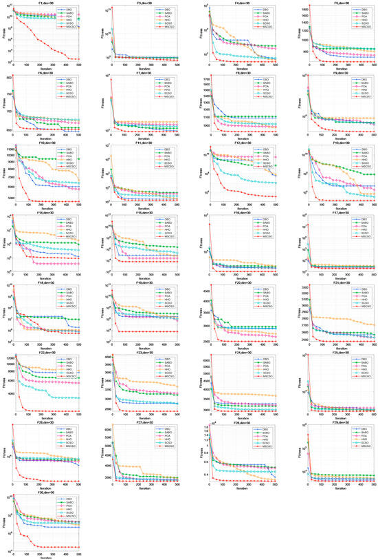
Figure A1.
Thirty-dimensional convergence curves of six optimization algorithms.
Figure A1.
Thirty-dimensional convergence curves of six optimization algorithms.
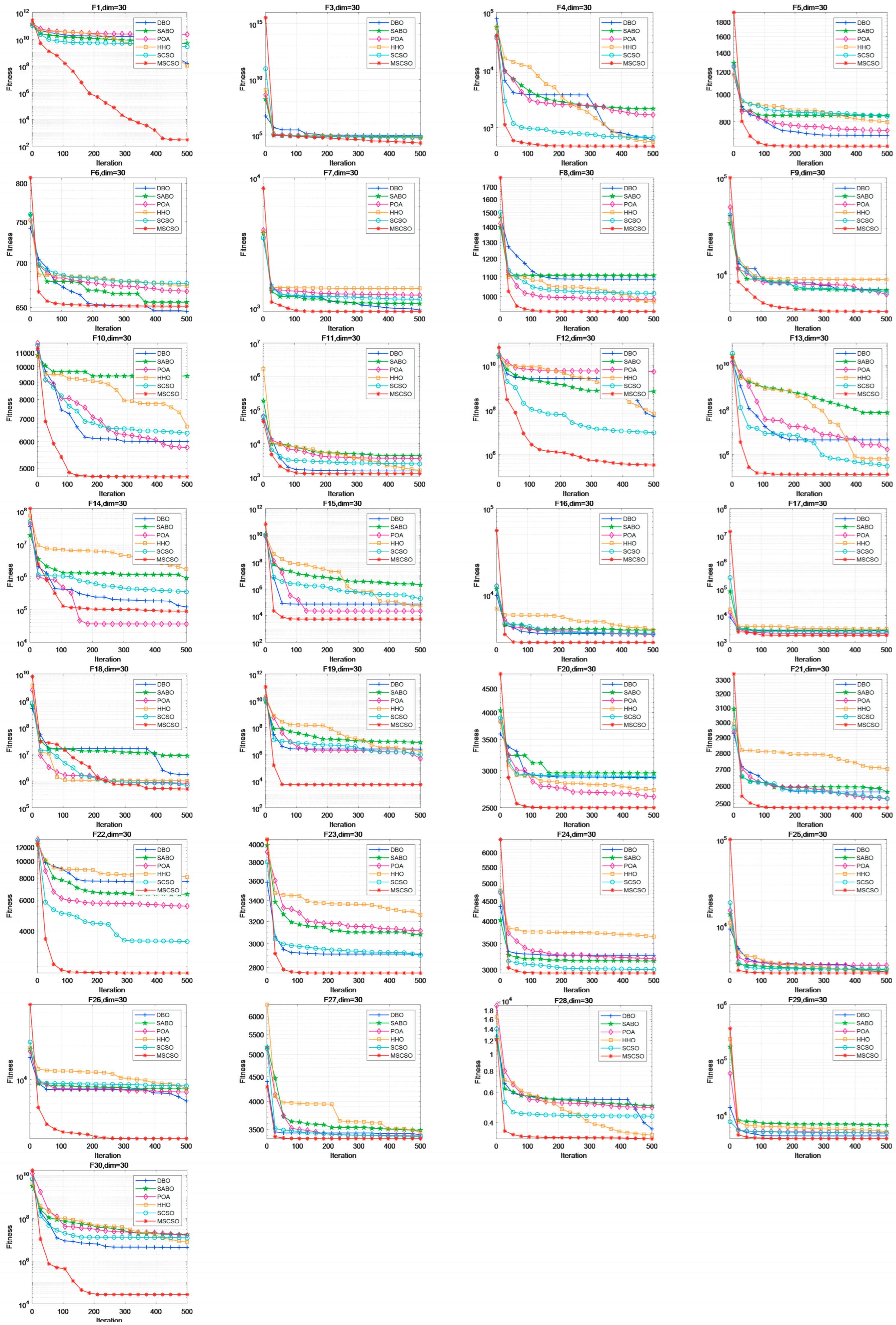
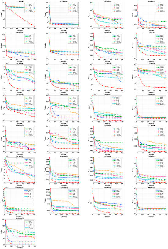
Figure A2.
Fifty-dimensional convergence curves of six optimization algorithms.
Figure A2.
Fifty-dimensional convergence curves of six optimization algorithms.
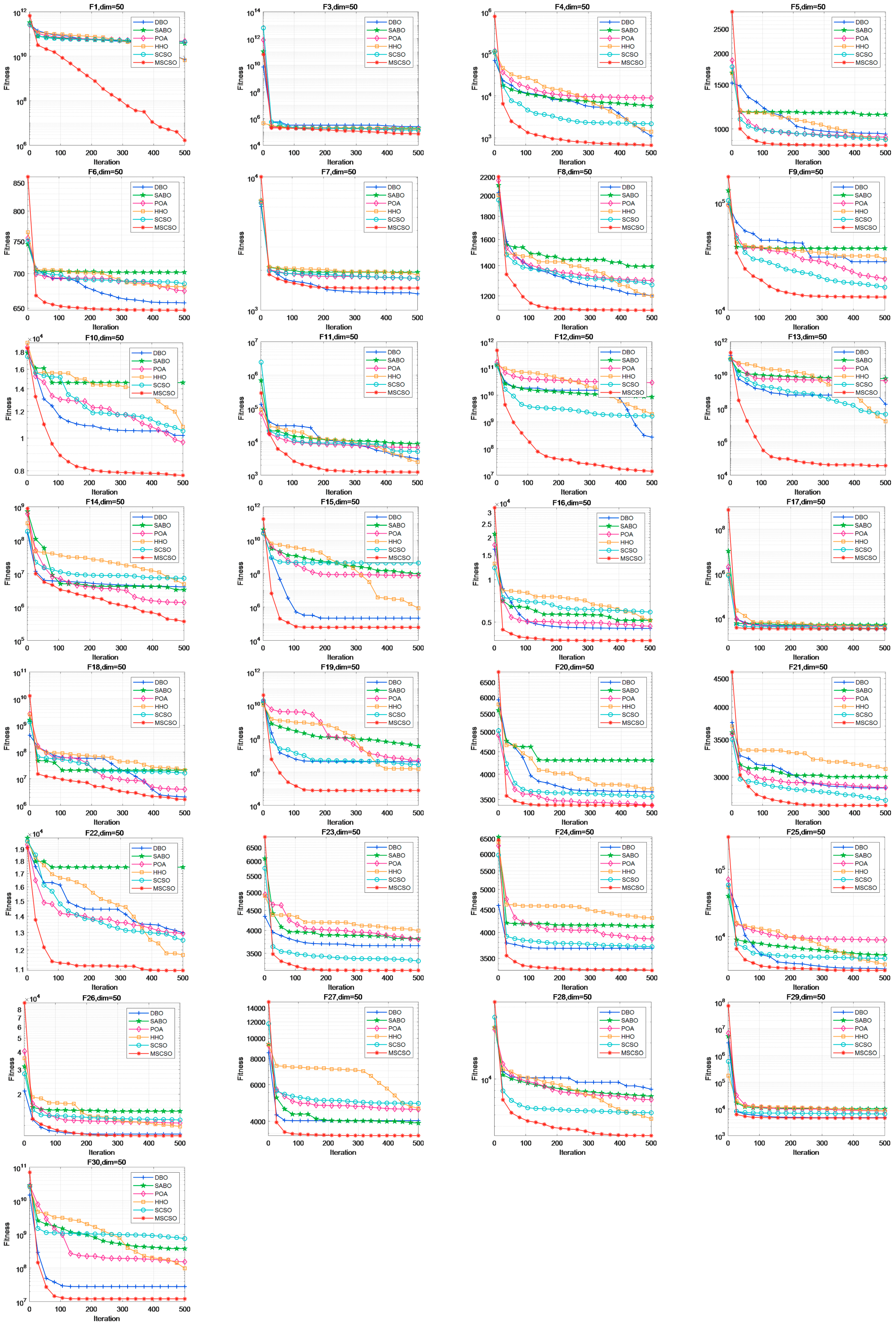
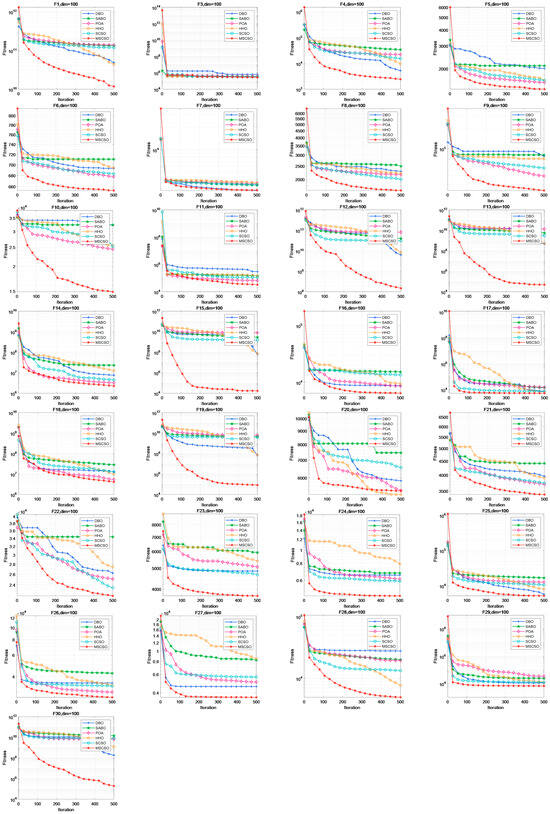
Figure A3.
One-hundred-dimensional convergence curves of six optimization algorithms.
Figure A3.
One-hundred-dimensional convergence curves of six optimization algorithms.
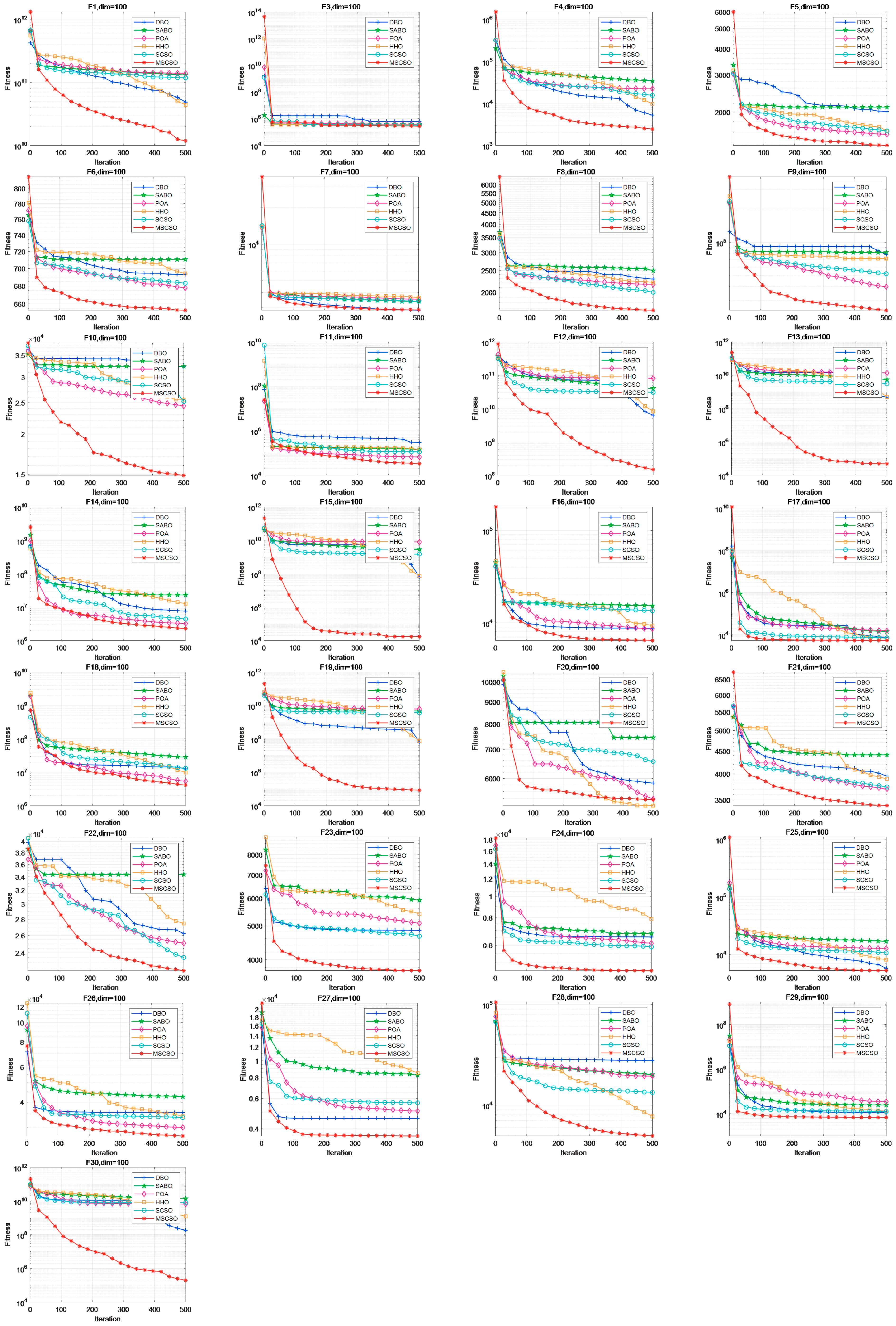
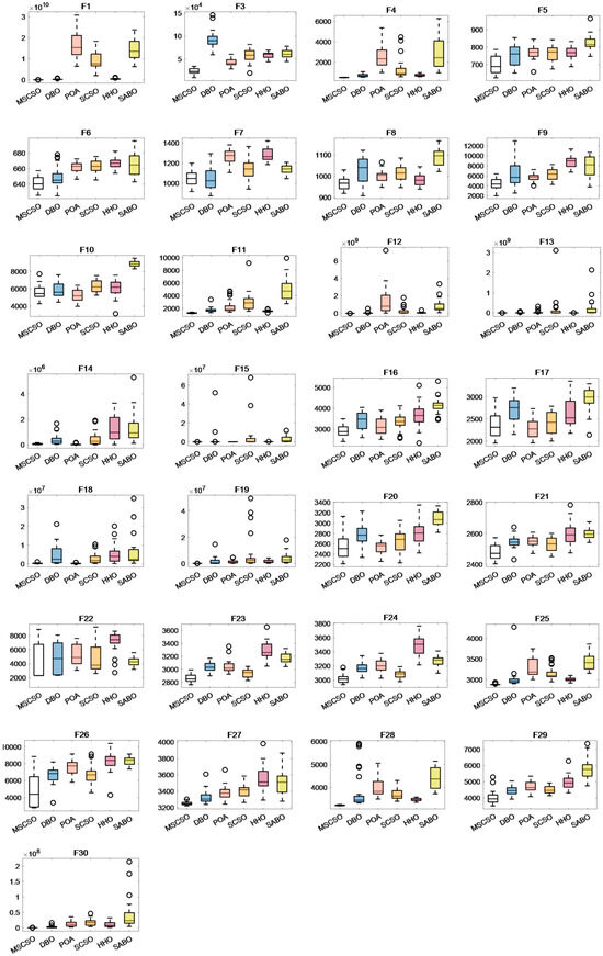
Figure A4.
Results of 30-dimensional box plots.
Figure A4.
Results of 30-dimensional box plots.
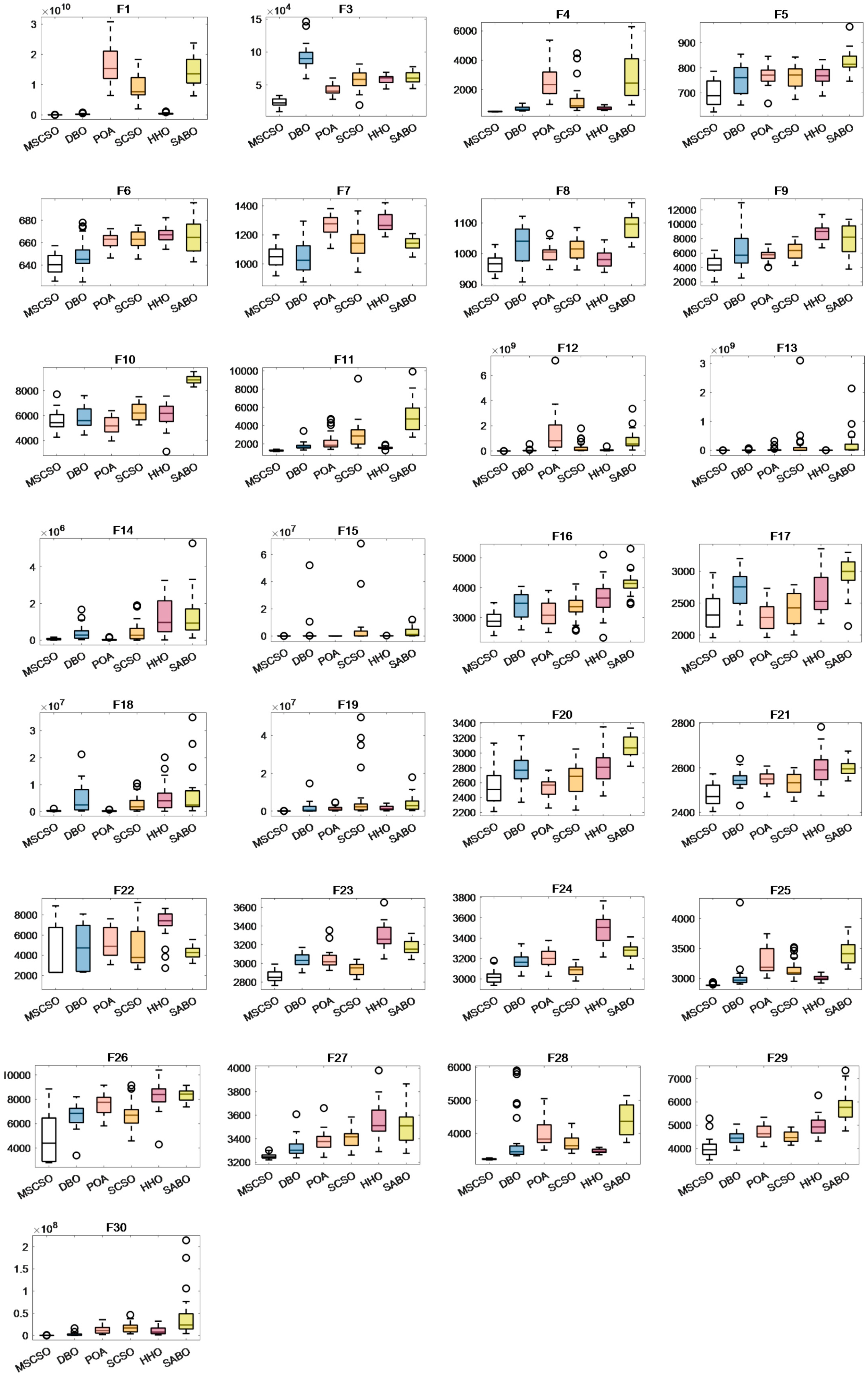
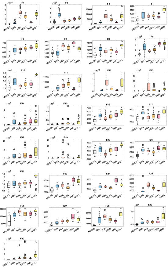
Figure A5.
Results of 50-dimensional box plots.
Figure A5.
Results of 50-dimensional box plots.
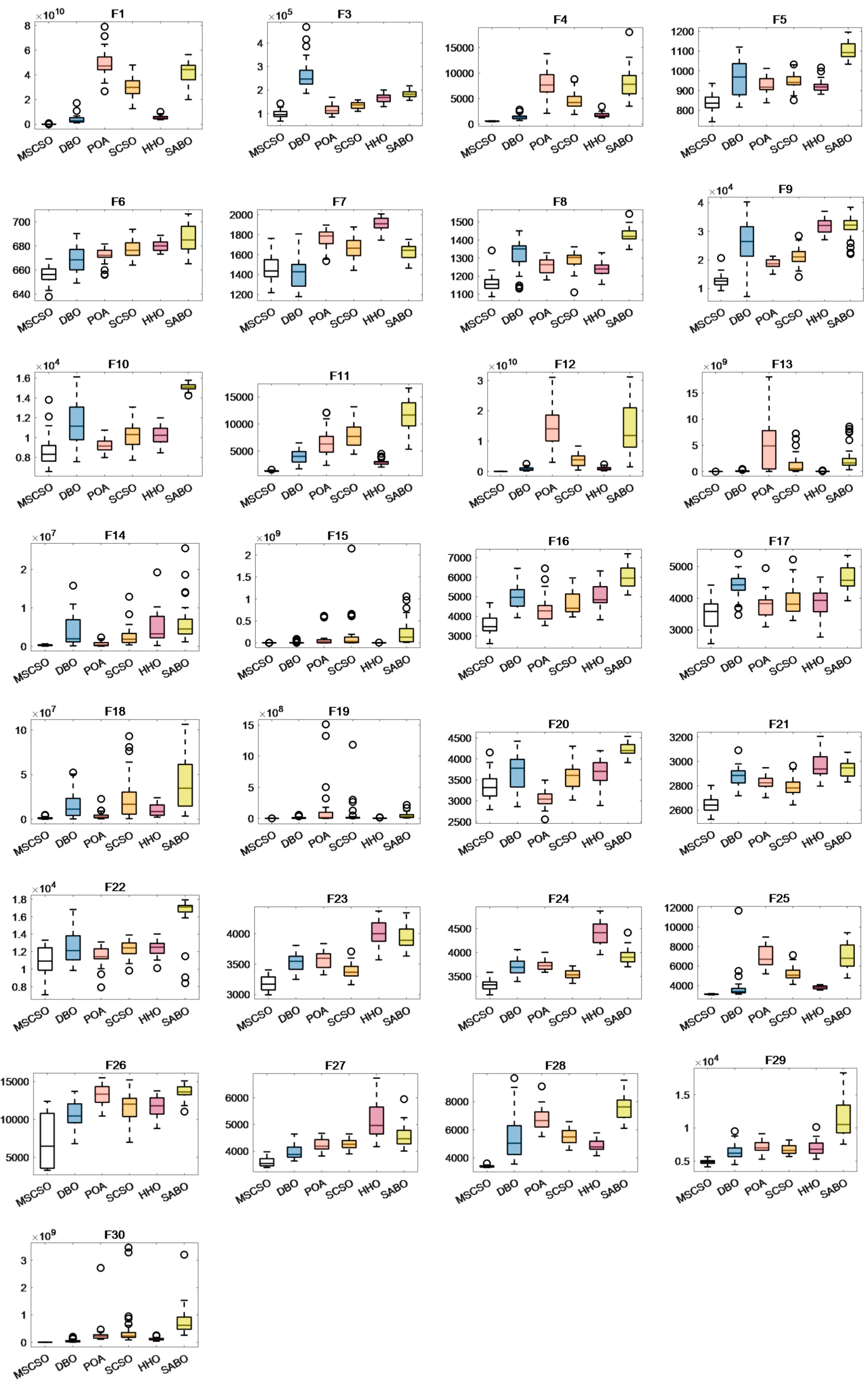
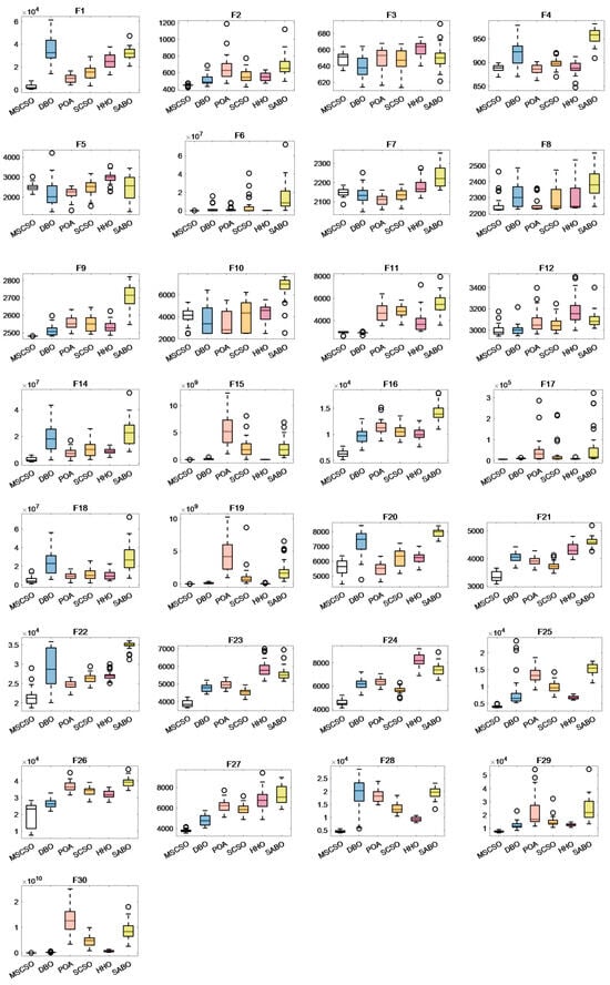
Figure A6.
Results of 100-dimensional box plots.
Figure A6.
Results of 100-dimensional box plots.
References
- Rezk, H.; Olabi, A.G.; Wilberforce, T.; Sayed, E.T. Metaheuristic optimization algorithms for real-world electrical and civil engineering application: A Review. Results Eng. 2024, 23, 102437. [Google Scholar] [CrossRef]
- Jia, H. Design of fruit fly optimization algorithm based on Gaussian distribution and its application to image processing. Syst. Soft Comput. 2024, 6, 200090. [Google Scholar] [CrossRef]
- Aishwaryaprajna; Kirubarajan, T.; Tharmarasa, R.; Rowe, J.E. UAV path planning in presence of occlusions as noisy combinatorial multi-objective optimisation. Int. J. Bio-Inspired Comput. 2023, 21, 209–217. [Google Scholar] [CrossRef]
- Wang, K.; Guo, M.; Dai, C.; Li, Z.; Wu, C.; Li, J. An effective metaheuristic technology of people duality psychological tendency and feedback mechanism-based Inherited Optimization Algorithm for solving engineering applications. Expert Syst. Appl. 2024, 244, 122732. [Google Scholar] [CrossRef]
- Lan, F.; Castellani, M.; Zheng, S.; Wang, Y. The SVD-enhanced bee algorithm, a novel procedure for point cloud registration. Swarm Evol. Comput. 2024, 88, 101590. [Google Scholar] [CrossRef]
- Zhou, S.; Shi, Y.; Wang, D.; Xu, X.; Xu, M.; Deng, Y. Election Optimizer Algorithm: A New Meta-Heuristic Optimization Algorithm for Solving Industrial Engineering Design Problems. Mathematics 2024, 12, 1513. [Google Scholar] [CrossRef]
- Kennedy, J.; Eberhart, R. Particle swarm optimization. In Proceedings of the International Conference on Neural Networks 1995, Perth, WA, Australia, 27 November–1 December 1995; pp. 1942–1948. [Google Scholar]
- Dorigo, M. Positive Feedback as a Search Strategy; Technical Report; Dipartimento di Elettronica, Politecnico di Milano: Milan, Italy, 1991; pp. 16–91. [Google Scholar]
- Holland, J. Genetic algorithms. Sci. Am. 1992, 267, 66–72. [Google Scholar] [CrossRef]
- Xue, J.; Shen, B. A novel swarm intelligence optimization approach: Sparrow search algorithm. Syst. Sci. Control. Eng. 2020, 8, 22–34. [Google Scholar] [CrossRef]
- Xue, J.; Shen, B. Dung beetle optimizer: A new meta-heuristic algorithm for global optimization. J. Supercomput. 2023, 79, 7305–7336. [Google Scholar] [CrossRef]
- Trojovský, P.; Dehghani, M. Pelican optimization algorithm: A novel nature-inspired algorithm for engineering applications. Sensors 2022, 22, 855. [Google Scholar] [CrossRef]
- Heidari, A.A.; Mirjalili, S.; Faris, H.; Aljarah, I.; Mafarja, M.; Chen, H. Harris Hawks optimization: Algorithm and applications. Future Gener. Comput. Syst. 2019, 97, 849–872. [Google Scholar] [CrossRef]
- Trojovský, P.; Dehghani, M. Subtraction-average-based optimizer: A new swarm-inspired metaheuristic algorithm for solving optimization problems. Biomimetics 2023, 8, 149. [Google Scholar] [CrossRef] [PubMed]
- Seyyedabbasi, A.; Kiani, F. Sand Cat swarm optimization: A nature-inspired algorithm to solve global optimization problems Figure 3. Eng. Comput. 2023, 39, 2627–2651. [Google Scholar] [CrossRef]
- Qiu, Y.; Zhou, J. Short-term rockburst damage assessment in burst-prone mines: An explainable XGBOOST hybrid model with SCSO algorithm. Rock Mech. Rock Eng. 2023, 56, 8745–8770. [Google Scholar] [CrossRef]
- Aghaei, V.T.; SeyyedAbbasi, A.; Rasheed, J.; Abu-Mahfouz, A.M. Sand cat swarm optimization-based feedback controller design for nonlinear systems. Heliyon 2023, 9, e13885. [Google Scholar] [CrossRef] [PubMed]
- Adegboye, O.R.; Feda, A.K.; Ojekemi, O.R.; Agyekum, E.B.; Khan, B.; Kamel, S. DGS-SCSO: Enhancing Sand Cat Swarm Optimization with Dynamic Pinhole Imaging and Golden Sine Algorithm for improved numerical optimization performance. Sci. Rep. 2024, 14, 1491. [Google Scholar] [CrossRef] [PubMed]
- Niu, Y.; Yan, X.; Wang, Y.; Niu, Y. An improved sand cat swarm optimization for moving target search by UAV. Expert Syst. Appl. 2024, 238, 122189. [Google Scholar] [CrossRef]
- Seyyedabbasi, A. A reinforcement learning-based metaheuristic algorithm for solving global optimization problems. Adv. Eng. Softw. 2023, 178, 103411. [Google Scholar] [CrossRef]
- Kiani, F.; Nematzadeh, S.; Anka, F.A.; Findikli, M.A. Chaotic sand cat swarm optimization. Mathematics 2023, 11, 2340. [Google Scholar] [CrossRef]
- Kiani, F.; Anka, F.A.; Erenel, F. PSCSO: Enhanced sand cat swarm optimization inspired by the political system to solve complex problems. Adv. Eng. Softw. 2023, 178, 103423. [Google Scholar] [CrossRef]
- Wolpert, D.H.; Macready, W.G. No free lunch theorems for optimization. IEEE Trans. Evol. Comput. 1997, 1, 67–82. [Google Scholar] [CrossRef]
- Luogeng, H. Applications of Number Theory to Modern Analysis; Science Press: Beijing, China, 1978. [Google Scholar]
- Zhu, F.; Li, G.; Tang, H.; Li, Y.; Lv, X.; Wang, X. Dung beetle optimization algorithm based on quantum computing and multi-strategy fusion for solving engineering problems. Expert Syst. Appl. 2024, 236, 121219. [Google Scholar] [CrossRef]
- Qiu, Y.; Yang, X.; Chen, S. An improved gray wolf optimization algorithm solving to functional optimization and engineering design problems. Sci. Rep. 2024, 14, 14190. [Google Scholar] [CrossRef] [PubMed]
- Gao, P.; Ding, H.; Xu, R. Whale optimization algorithm based on skew tent chaotic map and nonlinear strategy. Acad. J. Comput. Inf. Sci. 2021, 4, 91–97. [Google Scholar] [CrossRef]
- Li, Q.; Shi, H.; Zhao, W.; Ma, C. Enhanced Dung Beetle Optimization Algorithm for Practical Engineering Optimization. Mathematics 2024, 12, 1084. [Google Scholar] [CrossRef]
- Derrac, J.; García, S.; Molina, D.; Herrera, F. A practical tutorial on the use of nonparametric statistical tests as a methodology for comparing evolutionary and swarm intelligence algorithms. Swarm Evol. Comput. 2021, 1, 3–18. [Google Scholar] [CrossRef]
- Bayzidi, H.; Talatahari, S.; Saraee, M.; Lamarche, C.P. Social network search for solving engineering optimization prob lems. Comput. Intell. Neurosci. 2021, 2021, 8548639. [Google Scholar] [CrossRef]


Disclaimer/Publisher’s Note: The statements, opinions and data contained in all publications are solely those of the individual author(s) and contributor(s) and not of MDPI and/or the editor(s). MDPI and/or the editor(s) disclaim responsibility for any injury to people or property resulting from any ideas, methods, instructions or products referred to in the content. |
© 2024 by the authors. Licensee MDPI, Basel, Switzerland. This article is an open access article distributed under the terms and conditions of the Creative Commons Attribution (CC BY) license (https://creativecommons.org/licenses/by/4.0/).