Generalizations of Rolle’s Theorem

Abstract

The classical Rolle’s theorem establishes the existence of (at least) one zero of the derivative of a continuous one-variable function on a compact interval in the real line, which attains the same value at the extremes, and it is differentiable in the interior of the interval. In this paper, we generalize the statement in four ways. First, we provide a version for functions whose domain is in a locally convex topological Hausdorff vector space, which can possibly be infinite-dimensional. Then, we deal with the functions defined in a real interval: we consider the case of unbounded intervals, the case of functions endowed with a weak derivative, and, finally, we consider the case of distributions over an open interval in the real line.

1. Introduction

The celebrated Rolle’s theorem, familiar to undergraduate students in Analysis (see, e.g., [1] just to quote a book, or the book by the second author [2]), can be stated as follows:

Let f be a function that is continuous on the closed interval $[a,b]$ and differentiable on the open interval $]a,b[$. If $f\left(a\right)=f\left(b\right)$, then there exists a point c in $]a,b[$ for which $f^{\prime }\left(c\right)=0$.

This theorem appeared in a primitive form in a book dated 1690 (see a translation in [3]), and it has an interesting story (see [4,5,6]) because Rolle is known paradoxically for his attack on infinitesimal calculus for its “lack of rigour”. Since its first appearance, it has attracted the attention of researchers, who have published generalizations in several directions, variants, or also less-standard proofs (see, e.g., a constructive proof in [7]). It had a role in all the levels of study in Mathematics, from school instruction (see, e.g., the experiments in Nepal [8]) to some variants of interest for first-year calculus classes ([9,10,11]) and for second-year calculus classes ([12]) until dynamical systems (see, e.g., [13]). A large body of literature concerns the functions defined in more abstract structures. For instance, the theorem has been considered for complex valued functions in the framework of the complex plane (see, e.g., [14,15,16,17]) and for functions defined in finite-dimensional spaces (see, e.g., [18]). Moreover, there exists an “approximate version” for the functions defined in the closure of open connected bounded sets in Banach spaces (see [19,20,21]) because Rolle’s theorem cannot be applied to the functions defined in the closure of the unit ball in infinite-dimensional Banach spaces, where continuous functions may not have minimum and maximum values (because compactness is lost; see, e.g., [22] and the references therein, and also [23]). At last, we mention a version for real functionals defined in a whole real Banach space, which appears in [24], a study on the range of the derivative of functions with bounded support in [25], and the recent contributions [26,27,28,29,30,31,32].

The aim of this paper is to prove four results that generalize the classical result.

First, we point out that Rolle’s theorem has much broader validity than the classical theorem; in fact, it can be applied to functions whose domain is a closed set endowed with interior points, of any locally convex topological Hausdorff vector space (see the precise statement of Theorem 1); in particular, as already known, it can be applied to real functions of several variables, and to functions of a single variable not necessarily defined in an interval. Then, with reference to the functions defined in an interval of $\mathbb{R}$, the classical theorem is generalized from different points of view.

The second result (see Theorem 2) shows that, in Rolle’s theorem, the function can also be defined in an unbounded interval under the assumption that the limits in the extremes, assumed to exist, are equal (see Figure 1); we do not exclude that there exist points at which the function has an infinite derivative (see Figure 2), and, moreover, when it is finite, there is no need for the continuity in the extremes; at last, there is also no need for the interval to be closed. As an application, we prove Theorem 3, which also generalizes Lagrange’s theorem.

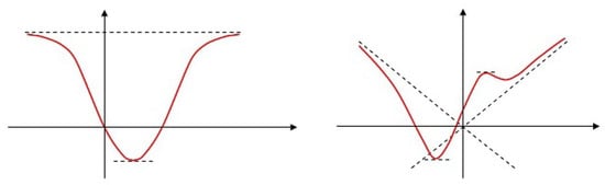
Figure 1. Unbounded intervals.

Figure 2. Bounded intervals.

If in Rolle’s theorem we assume the function of class $C^1$ (i.e., a continuous first derivative) in a compact interval, the integral mean of the derivative is equal to zero (it suffices to use the fundamental formula of integral calculus); this trivial observation suggests the thesis of the third theorem (see Theorem 4), which cannot be the same as that of Rolle’s theorem because the function, instead of being endowed with a derivative defined pointwise, is assumed to be endowed with a weak derivative belonging to $L^1$ (i.e., whose modulus is integrable).

Finally, Theorem 5 can be considered Rolle’s theorem for distributions over an open interval of $\mathbb{R}$.

2. The Main Results

We begin by recalling the classical notion of a Gateaux differential, which is a generalization of the concept of a directional derivative in differential calculus. Let S be a topological Hausdorff vector space, $\Omega$ be an open subset of S, and f be a real and continuous function defined in $\Omega$. For each $x_0\in \Omega$, the function f is said to be Gateaux-differentiable at the point $x_0\in \Omega$, where, for each $y\in S$, there exists a finite limit

$${\ell }_y=\underset{t\to 0}{lim}\frac{f(x_0+ty)-f\left(x_0\right)}{t},$$

and the map $y\in S\to {\ell }_y\in \mathbb{R}$ is a linear and continuous operator. If f is Gateaux-differentiable at the point $x_0$, then the map $y\in S\to {\ell }_y\in \mathbb{R}$ is denoted by $df\left(x_0\right)$, and it is called the Gateaux differential of f at the point $x_0$. In the particular case $S={\mathbb{R}}^n$, the Gateaux differentiability is equivalent to derivability according to any direction, and $df\left(x_0\right)$ is the differential of f in the classical sense.

By using the same argument as in calculus, we show that the following generalized Rolle’s theorem holds as follows:

Theorem 1.

Let S be a locally convex topological Hausdorff vector space, D a proper subset of S, closed and with nonempty interior; let f be a real function defined in D, continuous in D and Gateaux-differentiable in the interior points. Then, if f is constant on the boundary of D, and if there exist $minf$ and $maxf$ (for instance, in the case D is a compact set), then there exists at least one interior point $x_0$ of D such that $df\left(x_0\right)=0$.

Proof of Theorem 1.

Let us rule out the case that f is constant because, in such a case, the differential is zero for every interior point and the assertion is trivial.

By assumption, which is always satisfied in the case that D is a compact set, by the Weierstrass theorem (see, e.g., Theorem 4.16, p. 89 [33]), the function has a minimum and a maximum; let $x_0,x_1$ be points of D such that $f\left(x_0\right)=minf$ and $f\left(x_1\right)=maxf$. At least one of the points $x_0,x_1$, e.g., $x_0$, is interior to D; if they were both boundary points (note that the boundary of D is nonempty because D is a proper subset of S), by the assumption that f is constant on the boundary of D, it would be $minf=maxf$ and therefore the function f would be constant; i.e., this would be the eventuality ruled out above.

Now, since $x_0$ is point of local minimum for f interior to the domain of f, as we are going to recall, we have $df\left(x_0\right)=0$ and the assertion will be proved.

A point of local extreme interior in D is such that $df\left(x_0\right)=0$ and can be proved in the framework of locally convex topological Hausdorff vector spaces by an argument very close to the standard one; nevertheless, there are a few details.

Let $x_0\in D$ be, e.g., a point of local minimum. Since it is interior in D, there exists a neighborhood $I\ni x_0$, $I\subset D$, such that $f\left(x\right)\ge f\left(x_0\right)$$\forall x\in I$, and, since S is a locally convex topological space, there exists a convex neighborhood $I_c\ni x_0$, $I_c\subset I$, satisfying

$$f\left(x\right)\ge f\left(x_0\right)\forall x\in I_c;$$

(1)

on the other hand, by the continuity of the addition in the vector space S, we have

$$\underset{t\to 0}{lim}{x}_0+ty=x_0,$$

and therefore there exists $\delta >0$ such that $\left|t\right|<\delta \Rightarrow x_0+ty\in I_c$. By (1), we obtain

$$\left|t\right|<\delta \Rightarrow f(x_0+ty)-f\left(x_0\right)\ge 0,$$

so that, by the known argument involving signs (the ratio is nonnegative when $0<t<\delta$ and nonpositive when $-\delta <t<0$), we have (the existence of the limit is ensured by the assumption of differentiability)

$$\underset{t\to 0}{lim}\frac{f(x_0+ty)-f\left(x_0\right)}{t}=0.$$

Since y is arbitrary, we obtain $df\left(x_0\right)=0$. □

Remark 1.

 

1.  The requirement of the closure of D in the assumptions of Theorem 1 appears just for the sake of simplicity. In fact, the statement holds as well assuming only that the set of the boundary points of D that belong to D are nonempty; if such set consists of a singleton, obviously, the assumption of f to be constant on the boundary must be dropped.

2.  From Theorem 1, in the case $S={\mathbb{R}}^n$, $n>1$, we obtain the classical Rolle’s theorem extended to functions of several variables, and we stress that, in the case $n=1$, the classical assumption that the domain of the function is an interval can be dropped.

3.  In the special case in which S is a Hilbert space, by Riesz’s theorem, the linear operator $df\left(x_0\right)$ is identified with the gradient of f (element of S), and, therefore, in the assumptions of the theorem, there exists at least one point $x_0$ interior to D such that $f^{\prime }\left(x_0\right)=0$. Moreover, we note that Theorem 1 can also be applied in the framework of infinite-dimensional Hilbert spaces to a function defined in the non-compact domain $D=\{x\in S:\parallel x\parallel \le 1\}$; in fact, by (8.24 p. 267 [34]), the function $f\left(x\right)={\parallel x\parallel }^2$ is Fréchet-differentiable at every point, and, therefore, we hold that f is in particular Gateaux-differentiable. This is well-known; however, for the sake of completeness, we recall here the short proof. We will apply the fact that, for all $x\in S$, it is ${\parallel x\parallel }^2=x•x$, where by • we denote the scalar product in S. Since

$$\underset{t\to 0}{lim}\frac{f(x+ty)-f\left(x\right)}{t}=\underset{t\to 0}{lim}\frac{{\parallel x+ty\parallel }^2-{\parallel x\parallel }^2}{t}=\underset{t\to 0}{lim}\frac{(x+ty)•(x+ty)-{\parallel x\parallel }^2}{t}$$

$$=\underset{t\to 0}{lim}\frac{t^2{\parallel y\parallel }^2+2tx•y}{t}=\underset{t\to 0}{lim}{t\parallel y\parallel }^2+2x•y=2x•y,$$

we have

$$df\left(x\right):y\in S\to 2x•y.$$

The value of f is 1 on the boundary of D, and, in this case, the point $x=0$ is minimum for f and $df\left(0\right)=0$.

4.  The existence of $minf$ and $maxf$, which appear in the assumptions of Theorem 1, is essential for the validity of the thesis. In fact, if we denote by $D^{\prime }$ the closure of the complementary set of the unitary ball D considered in the previous point  3., the function

$$g:x\in D^{\prime }\to {\parallel x\parallel }^2$$

satisfies all the assumptions of Theorem 1 except the existence of the maximum, and no point $x_0$ exists, interior to $D^{\prime }$, such that $dg\left(x_0\right)=0$. It should be noted that, if $x_0,y_0\in S\setminus \left\{0\right\}$, and $x_0$ interior to $D^{\prime }$ are orthogonal, we have $<dg\left(x_0\right),y_0>=2x_0•y_0=0$, but the thesis states that the whole operator $df\left(x_0\right)$ is identically zero.

5.  We stress that Theorem 1 can be applied not only in the framework of Hilbert spaces but also in a class of Banach spaces (which again, as in the previous point  3., can be infinite-dimensional). Namely, from Theorem 8.13 p. 247, [34], we know that every separable Banach space admits an equivalent norm that is Gateaux-differentiable in every point $x\ne 0$. This implies that the function $f\left(x\right)={\parallel x\parallel }^2$ is Gateaux-differentiable at every point (see, e.g., 8.18 p. 265, [34]), and, therefore, the same example shown in the previous point   3.  works also in this case.

6.  Recently ([35]), Rolle’s theorem has been extended to functions of several variables using a new definition of differentiability, which allows the thesis to be obtained even for points not necessarily interior to the domain.

7.  The conclusion of Theorem 1 still holds in the case of real functions that are continuous and Fréchet-differentiable in the interior points because, as already observed, they are also Gateaux-differentiable and the Fréchet differential equals the Gateaux differential.

Theorem 2.

Let f be a function defined in an interval $I\subseteq \mathbb{R}$ (closed, open, or semi-open) of extremes a and b (not excluding $a=-\infty$, nor $b=+\infty$), continuous at interior points of I and endowed therein with a derivative, finite or not; in the extremes, let f be endowed with limit (finite or not).

If the limits

$$\underset{x\to a}{lim}f\left(x\right),\underset{x\to b}{lim}f\left(x\right)$$

(2)

are equal, then there exists at least one interior point $x_0$ of I such that $f^{\prime }\left(x_0\right)=0$.

Remark 2.

In Theorem 2, the assumption that f has derivative at all interior points is essential for the validity of the thesis (see Example 3 below).

Proof of Theorem 2.

In the proof, we will rule out the existence of an interval $I_1\subseteq I$ in which the function is constant since in such an eventuality the derivative is zero at all points of $I_1$ and therefore the thesis is trivially verified.

Denoted by ℓ, the limit of f in the extremes of I, we first prove that

$$\exists ]\alpha ,\beta [\subseteq I:f\left(x\right)\ne \ell \forall x\in ]\alpha ,\beta [$$

(3)

$$\underset{x\to \alpha }{lim}f\left(x\right)=\ell ,\underset{x\to \beta }{lim}f\left(x\right)=\ell .$$

(4)

In order to prove (3), we assume $\ell \ne \pm \infty$ because otherwise (3) is trivially verified with $\alpha =a$ and $\beta =b$. Having chosen a point $c\in ]a,b[$ such that $f\left(c\right)\ne \ell$ (it exists since f is not constant), let us consider the sets

$$A_c=\{t\in ]a,c[:f\left(x\right)\ne \ell \forall x\in ]t,c\left]\right\},B_c=\{t\in ]c,b[:f\left(x\right)\ne \ell \forall x\in [c,t]\};$$

since by continuity of f there exists a neighborhood of c in which the function does not take the value ℓ, such sets are nonempty, and setting

$$\alpha =inf{A}_c,\beta =sup{B}_c,$$

(5)

we have $\alpha <c<\beta$; we show that in $]\alpha ,\beta [$ the condition required in (3) is satisfied. On the contrary, let us assume that there exists $\xi \in ]\alpha ,\beta [\setminus \left\{c\right\}$ such that

$$f\left(\xi \right)=\ell .$$

(6)

If $\xi \in ]\alpha ,c[$, since $\xi$ is not a minorant of $A_c$, there exists $t\in A_c$ such that $t<\xi$; then, we have $f\left(\xi \right)\ne \ell$ (by the meaning of $t\in A_c$), which is in contrast with (6); on the other hand, if $\xi \in ]c,\beta [$, since $\xi$ is not a majorant of $B_c$, there exists $t\in B_c$ such that $t>\xi$; then, we have $f\left(\xi \right)\ne \ell$ (by the meaning of $t\in B_c$), which is in contrast with (6). Hence, (3) follows.

Now, in order to prove the first of (4), let us assume $\alpha >a$ (if $\alpha =a$, then the first of (4) holds because of the meaning of ℓ) so that $\alpha$ is an interior point of the interval I; then, by the continuity of f, the limit in the left-hand side exists and is equal to $f\left(\alpha \right)$; if it were $f\left(\alpha \right)\ne \ell$, there would exist $\delta >0$ such that $f\left(x\right)\ne \ell$$\forall x\in ]\alpha -\delta ,\alpha ]$ and therefore also $\forall x\in ]\alpha -\delta ,c]$; hence, it would be $(\alpha -\delta )\in A_c$ in conflict with the first of (5). By a similar argument, we can prove the second of (4).

Let us now denote by g the restriction of f to the interval $J=]\alpha ,\beta [$ so that from (4) we have

$$\underset{x\to \alpha }{lim}g\left(x\right)=\underset{x\to \beta }{lim}g\left(x\right)=\ell .$$

(7)

By the continuity of g, the range $g\left(J\right)$ is an interval since $\ell \ne g\left(J\right)$; the interval $g\left(J\right)$ is contained in one of the intervals $]-\infty ,\ell [$, $]\ell ,+\infty [$, precisely in the former if $\ell =+\infty$ and in the latter if $\ell =-\infty$ (we take these eventualities into account because it could be $[\alpha ,\beta ]=[a,b]$). It will suffice to examine the case $g\left(J\right)\subseteq ]-\infty ,\ell [$ since for the other case the argument is entirely analogous.

We will prove that, in the present case, the function g is endowed with a minimum, and that the minimum is attained at a point $x_0$ interior to J; after that, it will be easy to establish, by a classical argument, that $g^{\prime }\left(x_0\right)=0$. In the other case, where the proof is entirely analogous, the function is endowed with a maximum, attained at a point interior to J.

Setting $e_1=infg$ and $e_2=supg$, we have $e_1<e_2$; this is trivial if $e_1$ or $e_2$ is infinite; if both were finite, it would be $e_1=e_2$; the function would be constant, which we ruled out from the beginning.

Let us show that $\ell =e_2$, which is obvious if $\ell =+\infty$ since in such case the function is not upper-bounded; if $\ell \in \mathbb{R}$, having assumed $g\left(J\right)\subseteq ]-\infty ,\ell [$, the number ℓ is a majorant of g, and it is the minimum of majorants; in fact, by (7), taking into account the definition of limit, for every $\epsilon >0$, there exist points $x\in I$ such that $g\left(x\right)>\ell -\epsilon$.

Having shown that $\ell =e_2$, (7) becomes

$$\underset{x\to \alpha }{lim}g\left(x\right)=\underset{x\to \beta }{lim}g\left(x\right)=e_2.$$

(8)

On the other hand, if $e_1$ is finite [if $e_1=-\infty$], for every $n\in \mathbb{N}$, there exists $x_n\in J$ such that

$$e_1\le g\left(x_n\right)<e_1+\frac{1}{n}[g\left(x_n\right)<-n],$$

and therefore

$$\underset{n\to \infty }{lim}g\left(x_n\right)=e_1.$$

(9)

We may assume that the sequence $\left\{x_n\right\}$ is regular since there exists in any case a convergent or divergent extract sequence that can be denoted by the same symbol; hence, we are allowed to set $x_0={lim}_{n\to \infty }{x}_n$.

We show that $x_0$ is not an extreme of the interval $]\alpha ,\beta [$; if it were $x_0=\alpha$, since the limit of $g\left(x\right)$ exists as $x\to \alpha$ and $\left\{x_n\right\}$ is a sequence of points of the open interval $]\alpha ,\beta [$ having $\alpha$ as limit, by (9), we would have

$$\underset{x\to \alpha }{lim}g\left(x\right)=e_1,$$

which is contrary to (8) since $e_1<e_2$; similarly, we conclude that $x_0\ne \beta$.

Therefore, as to the point $x_0$ of the interval $]\alpha ,\beta [$, we have

$$\underset{n\to \infty }{lim}{x}_n=x_0,\underset{n\to \infty }{lim}g\left(x_n\right)=e_1;$$

hence, by the continuity of g,

$$g\left(x_0\right)=\underset{x\to x_0}{lim}g\left(x\right)=\underset{n\to \infty }{lim}g\left(x_n\right)=e_1.$$

Therefore, $g\left(x_0\right)$ is the minimum of the function g.

By assumption, the following limit exists (finite or infinite):

$$\underset{x\to x_0}{lim}\frac{g\left(x\right)-g\left(x_0\right)}{x-x_0}=g^{\prime }\left(x_0\right)=f^{\prime }\left(x_0\right),$$

and we can conclude that $f^{\prime }\left(x_0\right)=0$; if it were $f^{\prime }\left(x_0\right)>0$[$f^{\prime }\left(x_0\right)<0$], there would exist a neighborhood $I_1\subseteq I$ such that in $I_1\setminus \left\{x_0\right\}$ the difference quotient of g would be positive [negative], which is absurd because the numerator is nonnegative while the denominator is positive for $x>x_0$ and negative for $x<x_0$. The theorem is thus acquired. □

Example 1.

The function f, known as the Witch of Agnesi, defined by (see, e.g., [36])

$$f:x\in \mathbb{R}\to f\left(x\right)=\frac{1}{1+x^2},$$

satisfies the assumptions of Theorem 2. We note that $f^{\prime }\left(0\right)=0$.

Example 2.

The function $f:x\in \mathbb{R}\to \sqrt[3]{x^2-1}$ satisfies the assumptions of Theorem 2. We note that the derivative is infinite in the points $-1$, 1, and that $f^{\prime }\left(0\right)=0$.

Example 3.

The function $f:x\in [-1,1]\to \left|x\right|$ satisfies the assumptions of Rolle’s theorem except for the existence of the derivative at every point inside the definition interval since at point 0 (only at point 0) f is not derivable. The example proves that the thesis cannot hold because the derivative function of f is not zero at any point.

The standard application of Rolle’s theorem is Lagrange’s theorem with distinct limits in the extremes of the interval of definition of f (in the case of equal limits, Lagrange’s theorem becomes exactly Rolle’s theorem). In an analogous fashion, we have

Theorem 3.

Let f be a function defined in a bounded interval $I\subseteq \mathbb{R}$ (closed, open, or semi-open) of extremes a and b, continuous at interior points of I and endowed therein with the derivative function having a limit (finite or not) at every point of $[a,b]$, finite or not; in the extremes, let f be endowed with limit (finite or not).

If the limits

$$\underset{x\to a}{lim}f\left(x\right),\underset{x\to b}{lim}f\left(x\right)$$

(10)

are distinct, then there exists at least one point $\xi \in [a,b]$ such that

$$\underset{x\to b}{lim}f\left(x\right)-\underset{x\to a}{lim}f\left(x\right)=(b-a)\underset{x\to \xi }{lim}{f}^{\prime }\left(x\right).$$

(11)

Remark 3.

 

1.  In Theorem 3, the assumption that the interval I is bounded is essential for the validity of the thesis (see Example 4 below).

Since each of the limits in (10) can be $\pm \infty$, it should be noted that the left-hand side of (11) is not an indeterminate form (recall that by assumption the two limits are distinct). Furthermore, if the point ξ is interior to the interval or it is an extreme belonging to the interval, the limit on the right-hand side is equal to $f^{\prime }\left(\xi \right)$, even if $f^{\prime }\left(\xi \right)=\pm \infty$; in fact, this can be deduced from the definition of derivative at the point ξ, applying L’Hospital’s theorem (see, e.g., Theorem 5.13 p. 109, [33]).

Moreover, it is obvious that, if ξ is an extreme of the interval and it does not belong to it, the function is not defined there and therefore it does not make sense to consider $f^{\prime }\left(\xi \right)$.

2.  If the limits in the left-hand side of (11) are finite and, at the interior points of I, the function f is derivable, the point ξ in the right-hand side is interior to $[a,b]$, and it is sufficient to apply Lagrange’s classical theorem to the continuous extension on $[a,b]$ of the restriction of f to $]a,b[$.

Proof of Theorem 3.

For any compact interval $[a^{\prime },b^{\prime }]\subset ]a,b[$, if f is derivable at the interior points of $[a,b]$, by the classical Lagrange’s theorem, there exists at least one point c interior to $[a^{\prime },b^{\prime }]$ such that

$$f\left(b^{\prime }\right)-f\left(a^{\prime }\right)=(b^{\prime }-a^{\prime })f^{\prime }\left(c\right);$$

we observe that this assertion is valid also in the case that there are points interior to $[a^{\prime },b^{\prime }]$ where the derivative of f is infinite; this can be proved, using Theorem 2 acquired above, by the same procedure usually carried out to prove the classical Lagrange’s theorem.

Now, for each $n\in \mathbb{N}$, $n>2/(b-a)$, let us consider the restriction of f to the compact interval $I_n=[a+1/n,b-1/n]\subset ]a,b[$; because of what has just been observed, there exists at least one point $c_n$ interior to $I_n$ such that

$$f\left(b-\frac{1}{n}\right)-f\left(a+\frac{1}{n}\right)=\left(b-a-\frac{2}{n}\right)f^{\prime }\left(c_n\right).$$

(12)

Since the subsequence $\left\{c_n\right\}$ is bounded because the interval I is bounded, we can assume that it is convergent (since in the opposite case we can replace $\left\{c_n\right\}$ by a convergent extract sequence); on the other hand, denoted by $\xi$ the limit of $\left\{c_n\right\}$, by our assumption, there exists ${lim}_{x\to \xi }{f}^{\prime }\left(x\right)$ so that the limit of the subsequence $\left\{f^{\prime }\left(c_n\right)\right\}$ also exists and we have

$$\underset{n\to \infty }{lim}{f}^{\prime }\left(c_n\right)=\underset{x\to \xi }{lim}{f}^{\prime }\left(x\right).$$

Therefore, from (12), passing to the limit as $n\to \infty$, we deduce (11), and the assertion is proved. □

Example 4.

The arcotangent function satisfies the assumptions of Theorem 3, except that the domain is bounded; it is immediate to see that for this function the thesis of the theorem does not hold. In fact, it asserts the existence of a point $\xi \in [-\infty ,+\infty ]$ for which

$$\underset{x\to +\infty }{lim}arctanx-\underset{x\to -\infty }{lim}arctanx=(+\infty )·\underset{x\to \xi }{lim}\frac{1}{1+x^2},$$

i.e.,

$$\pi =(+\infty )·\underset{x\to \xi }{lim}\frac{1}{1+x^2}.$$

(13)

If $\xi \in \mathbb{R}$, the limit on the right-hand side is a positive number and (13) is false, while, if $\xi =\pm \infty$, the limit is 0 and (13) does not make sense.

Considering the restriction of the arcotangent function at the interval $[0,+\infty [$, we obtain an example with the domain lower-bounded but not upper-bounded in which the thesis of the theorem does not hold. Analogously, we could consider the restriction of the arcotangent function at the interval $]-\infty ,0]$, obtaining an example with the domain upper-bounded but not lower-bounded.

Next result involves the well-known notion of weak derivative of a function f. For a given function $f\in L_{loc}^1\left(I\right)$ (i.e., f is in $L^1$ over all compact sets contained in the open interval $I\subseteq \mathbb{R}$), a function $w\in L_{loc}^1\left(I\right)$ is said to be weak derivative of f if

$${\int }_{I}w\phi =-{\int }_{I}f{\phi }^{\prime }\forall \phi \in C_0^{\infty }\left(I\right),$$

where, as usual, by $C_0^{\infty }\left(I\right)$, we denote the set of functions differentiable infinitely many times, and having compact support in the interior of I. Since this notion extends the classical notion of derivative and it agrees with the classical one whenever the classical derivative exists and is continuous (see, e.g., [37] and Theorem 6.10, p. 136, [38]), the function w, which can be proved to be uniquely determined, is denoted by the standard symbol $f^{\prime }$.

Theorem 4.

Let f be a continuous function at the interior points of the interval $(a,b)$ (closed, open, or half-open, and bounded or not bounded), endowed in $]a,b[$ with a weak derivative belonging to $L^1$. If f is convergent in the extremes of the interval and

$$\underset{x\to a}{lim}f\left(x\right)=\underset{x\to b}{lim}f\left(x\right),$$

(14)

then

$${\int }_a^b{f}^{\prime }=\underset{x\to b}{lim}f\left(x\right)-\underset{x\to a}{lim}f\left(x\right)$$

(15)

and therefore

$${\int }_a^b{f}^{\prime }=0.$$

Obviously, under the assumptions of the theorem, in the case the interval is bounded, the thesis means that the mean integral of $f^{\prime }$ is equal to zero.

In the special case in which $f^{\prime }$ has a continuous representative in $]a,b[$, let us again call it $f^{\prime }$; the thesis implies that there exists a point $x_0\in ]a,b[$ such that $f^{\prime }\left(x_0\right)=0$; hence, for such class of functions, Theorem 4 is a generalization of Rolle’s theorem.

Proof of Theorem 4.

Fixed two sequences $\left\{a_n\right\}$ and $\left\{b_n\right\}$ of points of $(a,b)$ such that $lim{a}_n=a$ and $lim{b}_n=b$; we will use the relation

$${\int }_a^b{f}^{\prime }={\int }_a^{a_n}{f}^{\prime }+{\int }_{b_n}^b{f}^{\prime }+{\int }_{a_n}^{b_n}{f}^{\prime }.$$

(16)

The function f, being endowed in $]a,b[$ with a weak derivative in the compact interval $[a_n,b_n]\subset ]a,b[$, is absolutely continuous; hence, it is derivable so there exists a set $X_n\subset [a_n,b_n]$ of null Lebesgue measure such that f is derivable in $[a_n,b_n]\setminus X_n$; consequently, setting $X_0={\cup }_{n\in \mathbb{N}}{X}_n$, the function f is derivable in every point of $(a,b)\setminus X_0$; hence, it is derivable a.e. in $(a,b)$. Denoting by $f^{\ast }$ the classical derivative of f, and by $f_0^{\prime }$ a representative of the class $f^{\prime }$ (which denotes the weak derivative of f), we have

$$f^{\ast }=f_0^{\prime }\mathrm{a}.\mathrm{e}.\mathrm{in}(a_n,b_n).$$

(17)

On the other hand, since in the interval $[a_n,b_n]$ the function f is an absolutely continuous function, primitive of $f^{\ast }$, we have ${\int }_{a_n}^{b_n}{f}^{\ast }={\left[f\left(x\right)\right]}_{a_n}^{b_n}$, and, therefore, by (17),

$${\int }_{a_n}^{b_n}{f}^{\prime }={\int }_{a_n}^{b_n}{f}_0^{\prime }={\int }_{a_n}^{b_n}{f}^{\ast }={\left[f\left(x\right)\right]}_{a_n}^{b_n}.$$

Hence, (16) becomes

$${\int }_a^b{f}^{\prime }={\int }_a^{a_n}{f}^{\prime }+{\int }_{b_n}^b{f}^{\prime }+[f\left(b_n\right)-f\left(a_n\right)].$$

Such relationship holds for every $n\in \mathbb{N}$, and, passing to the limit as $n\to \infty$ and taking into account (14), we obtain (15), and the theorem is proved. □

Example 5.

The function $f:x\in [-1,1]\to \left|x\right|$ does not satisfy the assumptions of Theorem 2 (see Example 3), but it satisfies the assumptions of Theorem 4 because its weak derivative is (see, e.g., Theorem 6.17, p. 152, [38])

$$f^{\prime }\left(x\right)=\left\{\begin{array}{cc}& 1\mathit{if}x\in ]0,1[\hfill \\ & -1\mathit{if}x\in ]-1,0[\hfill \end{array}\right..$$

We note that the integral of $f^{\prime }$ over $(-1,1)$ equals zero.

Remark 4.

The standard application of Rolle’s theorem is Lagrange’s theorem. In the assumptions of Theorem 4, and if, moreover, the interval $(a,b)$ is bounded, denoting by ${\mu }_f(a,b)$ the integral mean of $f^{\prime }$ in $(a,b)$, the thesis (15) can be written equivalently as

$$\frac{{\displaystyle \underset{x\to b}{lim}f\left(x\right)-\underset{x\to a}{lim}f\left(x\right)}}{b-a}={\mu }_f(a,b)$$

so that Theorem 4 is a generalization of Lagrange’s theorem because on the right-hand side the value of $f^{\prime }$ in a suitable point of $(a,b)$ (which would be meaningless) is replaced by the integral mean of $f^{\prime }$ in $(a,b)$. Hence, Theorem 4, with the further assumption of the boundedness of the interval, can also be considered an application of Rolle’s theorem.

Let us now denote by I an open interval of $\mathbb{R}$ and by $C_{0,0}^{\infty }\left(I\right)$ the following subspace of $C_0^{\infty }\left(I\right)$:

$$C_{0,0}^{\infty }\left(I\right)=\left\{\phi \in C_0^{\infty }\left(I\right):{\int }_I\phi =0\right\}.$$

We have

Theorem 5.

Let $I\subseteq \mathbb{R}$ be an open interval, T be a distribution over I, and $T^{\prime }$ be the derivative of T. If there exist ${\phi }_1,{\phi }_2\in C_0^{\infty }\left(I\right)$ such that ${\phi }_1-{\phi }_2\in C_{0,0}^{\infty }\left(I\right)$ and $T{\phi }_1=T{\phi }_2$, then there exists $\psi \in C_0^{\infty }\left(I\right)$ such that

$$T^{\prime }\psi =0.$$

(18)

Proof. 

Let $]a,b[$ denote the open interval I. We will prove the assertion setting $\psi$ equal to the primitive function of ${\phi }_1-{\phi }_2$ defined by

$$\psi \left(x\right)={\int }_a^x[{\phi }_1\left(t\right)-{\phi }_2\left(t\right)]dt\forall x\in ]a,b[.$$

In order to show that $\psi \in C_0^{\infty }\left(I\right)$, first, we observe that $\psi \in C^{\infty }\left(I\right)$. Then, denoted by $[a^{\prime },b^{\prime }]$, an interval in $]a,b[$ containing the supports of ${\phi }_1$ and ${\phi }_2$, it is obvious that $\psi \equiv 0$ in $]a,a^{\prime }]$; on the other hand, $\psi \equiv 0$ also in $]b^{\prime },b]$ because ${\phi }_1-{\phi }_2\in C_{0,0}^{\infty }\left(I\right)$, and, therefore, for each $x\in [b^{\prime },b[$, we have

$$\psi \left(x\right)={\int }_a^x[{\phi }_1\left(t\right)-{\phi }_2\left(t\right)]dt={\int }_a^b[{\phi }_1\left(t\right)-{\phi }_2\left(t\right)]dt-{\int }_x^b[{\phi }_1\left(t\right)-{\phi }_2\left(t\right)]dt=0.$$

Property (18) is a direct consequence of the definition of derivative of a distribution and of the assumption $T{\phi }_1=T{\phi }_2$; in fact, $T^{\prime }\psi =-T{\psi }^{\prime }=T({\phi }_2-{\phi }_1)=0$. □

At last, we highlight a special case of Theorem 5. Let $f\in L_{loc}^1\left(\right]a,b\left[\right)$ (i.e., f is $L^1$ over all compact sets contained in $]a,b[$), $T_f$ be the distribution on $]a,b[$ associated with f, i.e.,

$$T_f\phi ={\int }_a^{b}f\phi \forall \phi \in C_0^{\infty }\left(\right]a,b\left[\right),$$

and, finally, let $T_f^{\prime }$ be the derivative of $T_f$:

$$T_f^{\prime }:\phi \in C_0^{\infty }\left(\right]a,b\left[\right)\to -{\int }_a^{b}f{\phi }^{\prime },$$

that is, the derivative of f in the sense of distributions.

In the case $T=T_f$, Theorem 5 reads as follows.

Theorem 6.

Let $f\in L_{loc}^1\left(\right]a,b\left[\right)$. If ${\phi }_1,{\phi }_2\in C_0^{\infty }\left(\right]a,b\left[\right)$ are such that ${\phi }_1-{\phi }_2\in C_{0,0}^{\infty }\left(I\right)$ and

$${\int }_a^{b}f{\phi }_1={\int }_a^{b}f{\phi }_2,$$

then there exists $\psi \in C_0^{\infty }\left(\right]a,b\left[\right)$ such that

$${\int }_a^{b}f{\psi }^{\prime }=0.$$

In particular, if f has a weak derivative, then there exists $\psi \in C_0^{\infty }\left(\right]a,b\left[\right)$ such that

$${\int }_a^b{f}^{\prime }\psi =0.$$

Example 6.

The functions

$$f\left(x\right)=\left\{\begin{array}{cc}& \left|x\right|\mathit{if}\left|x\right|<1\hfill \\ & 0\mathit{if}x\in ]-2,2[\setminus ]-1,1[\hfill \end{array}\right.,$$

$${\phi }_1\left(x\right)=\left\{\begin{array}{cc}& -exp\left(-\frac{1}{1-x^2}\right)\frac{2x}{{(1-x^2)}^2}\mathit{if}\left|x\right|<1\hfill \\ & 0\mathit{if}x\in ]-2,2[\setminus ]-1,1[\hfill \end{array}\right.,$$

and ${\phi }_2\equiv 0$ on $]-2,2[$ satisfy the assumptions of Theorem 6 after noticing that ${\phi }_1$ and $f{\phi }_1$ are odd functions. The expression of ${\phi }_1$ has been chosen to be equal to the derivative of the well-known Friedrichs mollifying kernel (see, e.g., p. 258, [39])

$$\psi \left(x\right)=\left\{\begin{array}{cc}& exp\left(-\frac{1}{1-x^2}\right)\mathit{if}\left|x\right|<1\hfill \\ & 0\mathit{if}x\in ]-2,2[\setminus ]-1,1[\hfill \end{array}\right.,$$

which is known to be $C_0^{\infty }\left(\right]-2,2\left[\right)$. We note that $f{\psi }^{\prime }=f{\phi }_1$ is odd, and, therefore,

$${\int }_{-2}^{2}f{\psi }^{\prime }=-{\int }_{-2}^2{f}^{\prime }\psi =0.$$

References

- Adams, R.A.; Essex, C. Calculus, Single Variable, 7th ed.; Prentice-Hall: Toronto, ON, Canada, 2009. [Google Scholar]
- Fiorenza, R.; Greco, D. Lezioni di Analisi Matematica, 3rd ed.; Liguori: Napoli, Italy, 1995. [Google Scholar]
- Smith, D.E. A Source Book in Mathematics; McGraw-Hill Book Co.: New York, NY, USA, 1929; Available online: https://archive.org/details/sourcebookinmath00smit/page/252/mode/2up (accessed on 8 April 2024).
- Robson, E.; Stedall, J. The Oxford Handbook of the History of Mathematics; Oxford University Press Inc.: New York, NY, USA, 2009. [Google Scholar]
- González, L.E. Comentarios históricos sobre el teorema de Rolle con referencias a la matemática española hacia 1911. Gaceta RSME 2011, 14, 167–178. [Google Scholar]
- Washington, C. Michel Rolle and His Method of Cascades; Mathematical Association of America: Washington, DC, USA, 2011. [Google Scholar]
- Abian, A. An ultimate proof of Rolle’s theorem. Am. Math. Mon. 1979, 86, 484–485. [Google Scholar] [CrossRef]
- Chaudhari, P.R.; Panthi, D.; Bhatta, C.R. Rolle’s theorem and its application in Tharu’s traditional house. Int. J. Phys. Math. 2023, 5, 13–17. [Google Scholar] [CrossRef]
- Luthar, R.S. View of Rolle’s theorem. Am. Math. Mon. 1969, 76, 680–681. [Google Scholar] [CrossRef]
- Gentry, R.D. Rolle’s theorem in elementary Calculus. Two-Year Coll. Math. J. 1973, 4, 11–17. [Google Scholar] [CrossRef]
- Samelson, H. On Rolle’s theorem. Am. Math. Mon. 1979, 86, 486. [Google Scholar] [CrossRef]
- Tineo, A. A generalization of Rolle’s theorem and an application to a nonlinear equation. J. Austral. Math. Soc. 1989, 46, 395–401. [Google Scholar] [CrossRef]
- Rousseau, C. Rolle’s Theorem: From a Simple Theorem to an Extremely Powerful Tool; Université de Montreal: Montreal, QC, Canada, 2011. [Google Scholar]
- Cater, F.S. Another application of Rolle’s theorem. Real Anal. Exch. 2004, 30, 795–798. [Google Scholar] [CrossRef]
- Evard, J.C.; Jafari, F. A complex Rolle’s theorem. Am. Math. Mon. 1992, 99, 858–861. [Google Scholar] [CrossRef]
- Khovanskii, A.; Yakovenko, S. Generalized Rolle theorem in Rn and C. J. Dynam. Contr. Syst. 1996, 2, 103–123. [Google Scholar] [CrossRef]
- Sendov, B. Complex analogues of the Rolle’s theorem. Serdica Math. J. 2007, 33, 387–398. [Google Scholar]
- Furi, M.; Martelli, M. A multidimensional version of Rolle’s theorem. Am. Math. Mon. 1995, 102, 243–249. [Google Scholar] [CrossRef]
- Azagra, D.; Deville, R. Subdifferential Rolle’s and mean value inequality theorems. Bull. Austral. Math. Soc. 1997, 56, 319–329. [Google Scholar] [CrossRef]
- Azagra, D.; Ferrera, J.; López-Mesas, F. Approximate Rolle’s theorems for the proximal subgradient and the generalized gradient. J. Funct. Anal. 2005, 220, 304–361. [Google Scholar] [CrossRef]
- Azagra, D.; Gómez, J.; Jaramillo, J.A. Rolle’s Theorem and Negligibility of Points in Infinite Dimensional Banach Spaces. J. Math. Anal. Appl. 1997, 213, 487–495. [Google Scholar] [CrossRef][Green Version]
- Azagra, D.; Jiménez-Sevilla, M. The Failure of Rolle’s Theorem in Infinite-Dimensional Banach Spaces. J. Funct. Anal. 2001, 182, 207–226. [Google Scholar] [CrossRef]
- Ferrer, J. Rolle’s theorem fails in ℓ2. Am. Math. Mon. 1996, 103, 161–165. [Google Scholar]
- e Silva, E.A.d.B.; Teixeira, M.A. A version of Rolle’s theorem and applications. Bol. Soc. Brasil. Mat. 1998, 29, 301–327. [Google Scholar] [CrossRef]
- Gaspari, T. On the range of the derivative of a real-valued function with bounded support. Studia Math. 2002, 153, 81–99. [Google Scholar] [CrossRef]
- Batts, L.J.; Moran, M.E.; Taylor, C.K. Extensions of Rolle’s theorem. Involv. J. Math. 2022, 15, 641–648. [Google Scholar] [CrossRef]
- Fan, Z.; Fu, Y.; Xu, H. Unravelling Three Differential Mean Value Theorems in Calculus. Highlights Sci. Eng. Technol. 2024, 88, 790–795. [Google Scholar] [CrossRef]
- Martínez-Legaz, J.E. A Mean Value Theorem for Tangentially Convex Functions. Set-Valued Var. Anal. 2023, 31, 13. [Google Scholar] [CrossRef]
- Zajac, K. Generalized Lagrange Theorem. J. Math. Anal. Appl. 2024, 531, 127890. [Google Scholar] [CrossRef]
- Zakaria, M.; Moujahid, A.; Ikhouba, M. A new fractional derivative operator and applications. Int. J. Nonlinear Anal. Appl. 2023, 14, 1277–1282. [Google Scholar]
- Zhou, Y. Mean Value Theorem and Its Uses. Highlights Sci. Eng. Technol. 2023, 72, 926–930. [Google Scholar] [CrossRef]
- Zhou, Y.; Gao, C.; Yu, W. Formal Proof of the Mean Value Theorem Based on Coq. In Proceedings of the 2023 China Automation Congress (CAC), Chongqing, China, 17–19 November 2023; pp. 5726–5730. [Google Scholar] [CrossRef]
- Rudin, W. Principles of Mathematical Analysis; McGraw-Hill, Inc.: New York, NY, USA, 1976. [Google Scholar]
- Fabian, M.; Habala, P.; Hájek, P.; Santalucía, V.M.; Pelant, J.; Zizler, V. Functional Analysis and Infinite-Dimensional Geometry; Springer: New York, NY, USA, 2001. [Google Scholar]
- Koceić-Bilan, N.; Mirošević, I.M. The Mean Value Theorem in the Context of Generalized Approach to Differentiability. Mathematics 2023, 11, 4294. [Google Scholar] [CrossRef]
- Yates, R.C. Witch of Agnesi. In Curves and Their Properties, Classics in Mathematics Education; National Council of Teachers of Mathematics: Reston, VA, USA, 1954; Volume 4, pp. 237–238. [Google Scholar]
- Valli, A. Weak Derivatives and Sobolev Spaces. In A Compact Course on Linear PDEs; Springer: Cham, Switzerland, 2021; Volume 154. [Google Scholar] [CrossRef]
- Lieb, E.H.; Loss, M. Analysis. In Graduate Studies in Mathematics; American Mathematical Society: Providence, RI, USA, 1997; Volume 14. [Google Scholar]
- diBenedetto, E. Real Analysis; Birkäuser Advanced Texts Series; Birkhäuser: Boston, MA, USA, 2002. [Google Scholar]
Disclaimer/Publisher’s Note: The statements, opinions and data contained in all publications are solely those of the individual author(s) and contributor(s) and not of MDPI and/or the editor(s). MDPI and/or the editor(s) disclaim responsibility for any injury to people or property resulting from any ideas, methods, instructions or products referred to in the content. |
© 2024 by the authors. Licensee MDPI, Basel, Switzerland. This article is an open access article distributed under the terms and conditions of the Creative Commons Attribution (CC BY) license (https://creativecommons.org/licenses/by/4.0/).