Article

Research on Autonomous Manoeuvre Decision Making in Within-Visual-Range Aerial Two-Player Zero-Sum Games Based on Deep Reinforcement Learning

1
Equipment Management and UAV Engineering College, Air Force Engineering University, Xi’an 710051, China
2
National Key Lab of Unmanned Aerial Vehicle Technology, Air Force Engineering University, Xi’an 710051, China
*
Author to whom correspondence should be addressed.
Mathematics 2024, 12(14), 2160; https://doi.org/10.3390/math12142160
Submission received: 17 June 2024 / Revised: 4 July 2024 / Accepted: 7 July 2024 / Published: 10 July 2024

Abstract

:
In recent years, with the accelerated development of technology towards automation and intelligence, autonomous decision-making capabilities in unmanned systems are poised to play a crucial role in contemporary aerial two-player zero-sum games (TZSGs). Deep reinforcement learning (DRL) methods enable agents to make autonomous manoeuvring decisions. This paper focuses on current mainstream DRL algorithms based on fundamental tactical manoeuvres, selecting a typical aerial TZSG scenario—within visual range (WVR) combat. We model the key elements influencing the game using a Markov decision process (MDP) and demonstrate the mathematical foundation for implementing DRL. Leveraging high-fidelity simulation software (Warsim v1.0), we design a prototypical close-range aerial combat scenario. Utilizing this environment, we train mainstream DRL algorithms and analyse the training outcomes. The effectiveness of these algorithms in enabling agents to manoeuvre in aerial TZSG autonomously is summarised, providing a foundational basis for further research.

1. Introduction

Unmanned Aerial Systems (UASs) (see Glossary) are increasingly vital in modern life, primarily operating via ground station remote control with human oversight for tasks like reconnaissance, surveillance, and ground attacks. However, advancements in networked, information-based, and intelligent scenarios have reduced aerial response times and intensified manoeuvres beyond human capabilities [1]. Enhancing UAS intelligence is crucial to adapting and gaining an advantage in aerial engagements. This involves enabling UASs to autonomously generate control commands based on situational awareness for aerial combat, making UAS intelligence a key future research direction.
Autonomous decision making is essential for the effectiveness of UASs, involving the real-time generation of optimal tactical commands in complex aerial combat environments [2,3,4,5]. While various zero-sum game decision-making methods have shown success under specific conditions, comprehensive methods for different scenarios and intelligent agents remain undeveloped [6]. The current methods are categorised into traditional and intelligent decision-making approaches.
Traditional autonomous decision-making methods include differential and matrix game methods [7,8,9], expert systems [10,11,12,13], and influence diagrams [14]. Recent advancements include Soltanifar [15], Farajpour Khanaposhtani [16], Ismail et al. [17], and Hosseini Nogourani et al. [18], focusing on multi-attribute decision making, support vector machines, DEMATEL with Bonferroni mean aggregation, and decision making under uncertainty and risk. However, these methods often suffer from high computational demands, reliance on manually set rules, and inflexibility. Reinforcement learning (RL), based on Markov decision processes (MDP), addresses these issues by enabling agents to interact with the environment and optimize strategies through feedback. Though suitable for finite MDPs, RL struggles with continuous spaces. Deep reinforcement learning (DRL) [19,20,21,22,23] combines deep learning’s perception capabilities with RL’s decision making, proving effective for complex problems like aerial manoeuvre decision making. Pan Y et al. [24] used DRL for zero-sum game scenarios with a dual-network Deep Q-network (DQN). Liu P et al. [25] applied DQN for continuous state inputs. Zhang Q et al. [26] used DQN for beyond-visual-range scenarios, addressing the Nash equilibrium. B. Kurniawan et al. [27] introduced the Actor–Critic (AC) architecture for improved training efficiency. Yang Q et al. [28,29] employed the Deep Deterministic Policy Gradient (DDPG) algorithm for continuous action outputs, enhancing control precision and smoothness.
This paper particularly focuses on Witness Visual Range (WVR) (see Glossary) scenarios due to their unique challenges, such as real-time decision making and high-speed manoeuvring. These complexities necessitate advanced decision algorithms. This paper advances research in deep reinforcement learning for close-range aerial zero-sum games (WVR). Key contributions include (1) establishing a kinematic model and a coarse-grained effective capture region model for WVR aerial zero-sum games; (2) constructing an MDP model for WVR games, facilitating deep reinforcement learning with reward shaping to address sparse rewards in autonomous manoeuvre decision making; (3) incorporate aerial agent manoeuvring into flight control mechanisms modelled on a typical UAS to expand the operational space and enhance AI exploration. A typical WVR aerial two zero-sum games (TZSGs) (see Glossary) is designed, and mainstream DRL algorithms are applied to a realistic simulation environment. The experimental results are analysed to summarise the characteristics of these algorithms and provide insights for further optimisation.

2. A Deep Reinforcement Learning Model for Manoeuvre Decision Making in WVR Aerial Agent Zero-Sum Games

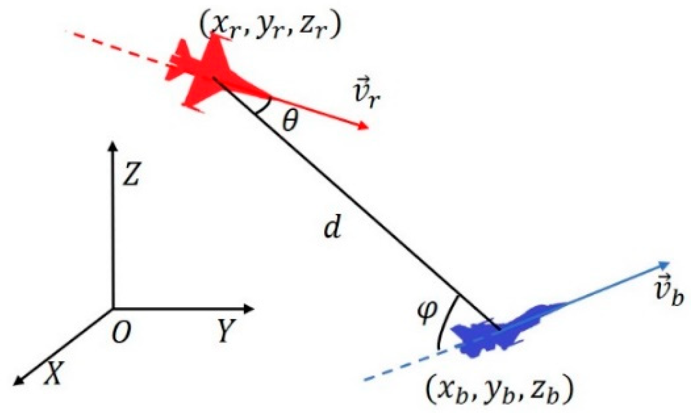
2.1. WVR Aerial Two-Player Zero-Sum Games Dynamics Modeling

Figure 1 illustrates the 1v1 WVR aerial TZSG model involving intelligent agents. Agent (r) represents our side, while agent (b) represents the opponent. The OXYZ coordinate system is a three-dimensional Cartesian coordinate system in which the origin O denotes the coordinate origin, typically located within the defined engagement area. In this context, the geometric centre of the aerial combat zone serves as the origin. The positive X-axis points east, the positive Y-axis points north, and the positive Z-axis points vertically upward.
As shown in Figure 1, assuming the zero angle of attack and sideslip angle, the agent’s velocity and body coordinate systems coincide, aligning the agent’s axis with its velocity direction. Agent (r) has velocity v r and position c R = x r , y r , z r . Agent (b) has velocity v b and position c B = x b , y b , z b . The distance d is the separation between agents (r) and (b). The target line connects their centres of mass. The target azimuth angle θ is the angle between v r and the target line, positive for rightward deviation, with 0 θ 180 . The target entry angle φ is the supplementary angle between v b and the target line, also positive for rightward deviation, with 0 φ 180 . The relative situation is described by c R , c B , d , θ , and φ :
d = c R c B 2 = x r x b 2 + y r y b 2 + z r z b 2
θ = arccos v R c B c R v R c B c R 180 π
φ = arccos v B c B c R v B c B c R 180 π

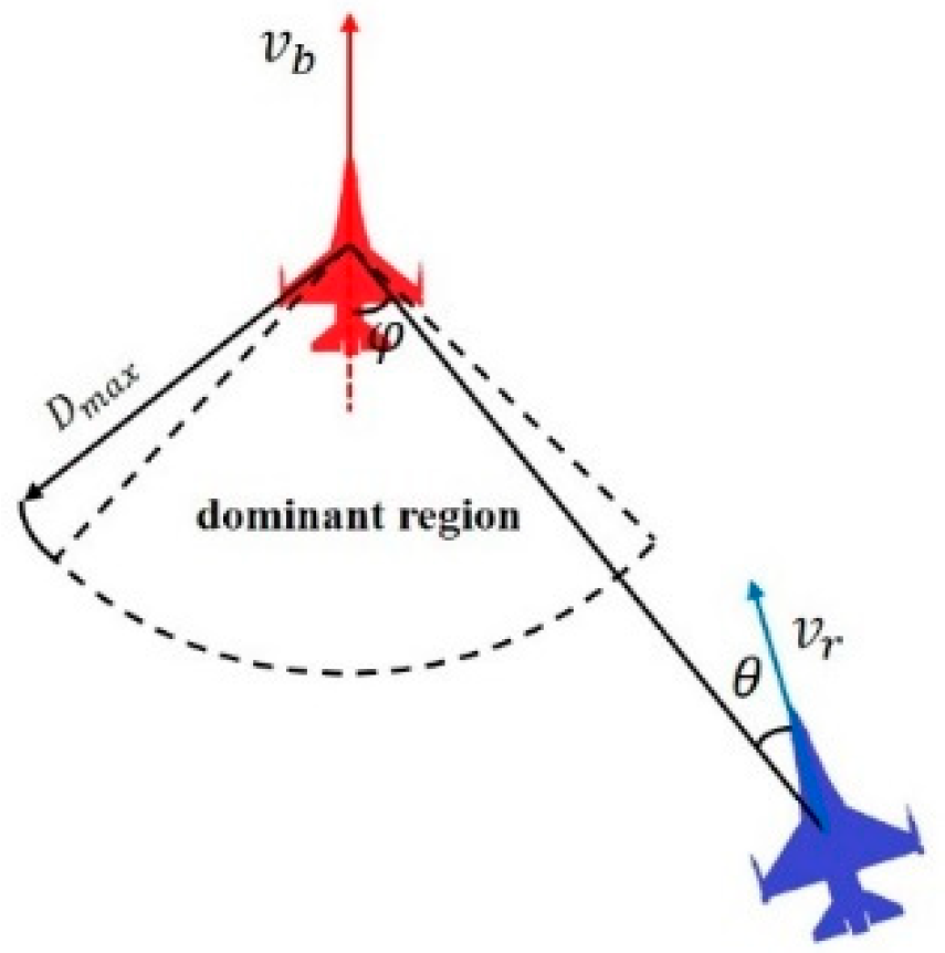
2.2. Capture Zone Modelling

The agent’s capture zone (see Glossary), which constrains manoeuvring decisions, is modelled using the radar radiation area centred on the agent, as shown in Figure 2. In Figure 2, D m a x and q m a x represent the maximum effective range and spread angle of the capture zone, respectively.
The maximum effective range D m a x and the maximum dispersion angle q m a x define the capture zone. It is independent of agent speed and target azimuth angle, changing only with the agent’s longitudinal axis. Both the distance and angle conditions must be met, as shown in Equation (4):
d D m a x θ q m a x
In the equation, d represents the distance between the red and blue agents, and θ denotes the target azimuth angle. Victory is achieved when any agent satisfies Equation (4).

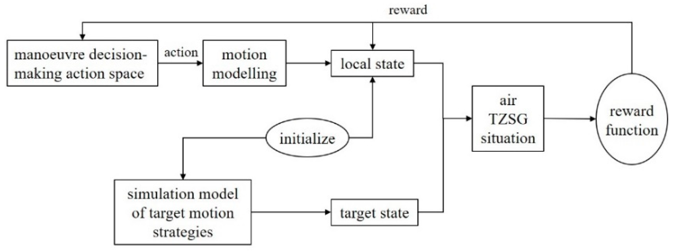
2.3. WVR Aerial TZSG MDP Modelling

In an aerial TZSG, an agent’s autonomous manoeuvring is modelled using a Markov decision process (MDP) defined by the quintuple S , A , P , r , γ . The agent interacts with the environment, obtaining state information s t S . Based on s t , the agent performs a manoeuvre a t A , receives a reward r s t , a t , and the environment updates to s t + 1 S . Assuming an ideal model with deterministic dynamics P s , a = 1 , the agent seeks a strategy π to maximize the cumulative reward 0 ɣ t r s t , a t a t = π s t where γ 0 , 1 is the discount factor.

2.3.1. State Space (S)

Based on the analysis of the agent’s WVR aerial TZSG model, as shown in Figure 1, the factors affecting the agent’s TZSG are the state characteristics of the fighters. These include the coordinates of the red agent c R = x r , y r , z r , the coordinates of the blue agent c B = x b , y b , z b , the speed of the red agent v r , the speed of the blue agent v b , the target azimuth θ , and the target entry angle φ . The state space of the agent’s WVR aerial TZSG manoeuvre decision making deep reinforcement learning model can be represented as follows:
S = x r , y r , z r , x b , y b , z b , v r , v b , θ , φ
Since the state space of a fighter aircraft is continuous and infinite, a deep learning neural network is required to process these features.

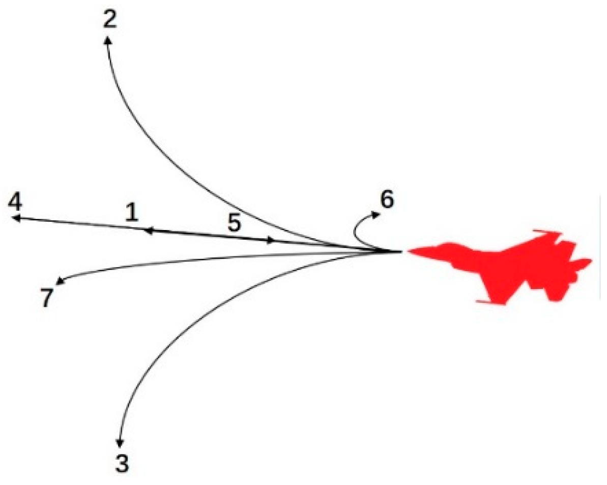
2.3.2. Action Space (A)

References [30,31] define seven fundamental manoeuvre actions for an agent’s flight states, forming a manoeuvre action library: (1) steady flight, (2) max load factor increase, (3) max load factor decrease, (4) max throttle increase, (5) max throttle decrease, (6) max roll angle increase, and (7) max roll angle decrease. This paper uses this library for game-theoretic decision making. The figure below shows these actions.
Figure 3 depicts that in one time step Δ t , the seven basic flight manoeuvres that a UAV can execute within a time step are as follows:
Using seven basic manoeuvre combinations simplifies calculations and allows for a flexible representation of most flight attitudes. The core of manoeuvre decision making is choosing the appropriate basic manoeuvre to maximise combat advantage in the current state.

2.3.3. Rewards

Training a manoeuvre guidance agent using deep reinforcement learning (DRL) in aerial zero-sum games faces two main challenges: the sparse reward problem, where success is only measured by achieving an advantageous position, leading to slow convergence, and the need to consider both the time to reach this position and the quality of the trajectory in practical scenarios. A reward-shaping method is proposed to address these issues and improve training speed and strategy performance.
Before reward shaping, advantageous locations/areas need to be defined.
Figure 4 illustrates the dominant region (see Glossary) in games according to the definition provided in the reference [4].
As shown in Figure 2, the smaller the red agent’s target azimuth angle θ , the easier it is for the blue agent to aim at and destroy the red agent, gaining a combat advantage. Conversely, when the red agent’s target entry angle φ is larger, it becomes harder for the red agent to aim at the blue agent, making the blue agent safer. Additionally, the capture zone of the agents is crucial. Reward shaping [32] is used to modify the reward function to promote learning while maintaining an optimal policy. In this study, the reward function is defined as follows:
(1)
Environmental reward function
The environmental reward function is shown below:
R e n v s = R T s + R C s
where R T s is the termination reward function given to the AI at the end game moment and R C s are the reward functions given to the basic information of the matchmaking, which are, respectively:
R T s = 100       R e d   W i n 100   B l u e   W i n 0         others
(2)
Shaping the reward function
A real-valued function R s i t u s is a function of the dominance of a state. The larger the value of this function, the more favourable the current situation is. This function can provide additional information to help the agent choose an action, which is better than using only termination rewards. It is defined as follows:
R s i t u s = t × R a s × R d s
The T-value is tentatively set at 100. We need to tune the parameter.
  • where R d s is the distance reward function, and R a s is the direction reward function, which are defined as
R a s = 1 ATA + AA 180
R d s = exp d t d m a x + d m i n / 6 180 k
where k is in metres/degrees, used to adjust the relative effect of distance and angle; the value is tentatively set to 10 needed to adjust the reference; in this case, d m a x = 1000 , d m i n = 10 .
(3)
Total reward function
R s = R s i t u s + R e n v s

3. Deep Reinforcement Learning Algorithms

3.1. Research Proposal

This paper advances the field by implementing deep reinforcement learning algorithms for WVR aerial TZSG manoeuvre decision making in three-dimensional space, addressing the limitations of current two-dimensional studies in the literature. The intelligent decision module effectively enhances the autonomy of aerial agents, improving mission efficiency and adaptability. Figure 5 illustrates the module, which evaluates the situation of agents and targets, inputs the data, and generates control commands to guide our agents.

3.2. Principles of Reinforcement Learning

Reinforcement learning (RL) uses a “trial and error” approach to interact with the environment, characterised by a Markov decision process [33]. It evaluates actions based on the cumulative payoff expectation, considering long-term effects. RL does not require training samples; only the environment’s return value is required. Thus, building a WVR aerial TZSG manoeuvre decision-making model using RL is feasible for autonomous decision making, as it generates decision sequences through self-interactive training.

3.3. Introduction to Deep Reinforcement Learning

Deep learning enables feature extraction directly from raw data via deep neural networks, excelling in feature representation but lacking in decision making. Conversely, reinforcement learning excels in decision making but is limited in perception. Consequently, DRL, which merges these two approaches, has become a research hotspot. DRL leverages trial and error, using rewards and punishments to adjust neural networks for optimal policy models.
Deep learning [34] refines data through representation learning without manual feature selection, achieving distributed data representation by combining low-level features into abstract high-level ones. Reinforcement learning [35], rooted in optimal control theory, addresses time-series decision making to maximise cumulative expected returns through continuous environment interaction.
Researchers use function approximation to address the dimensionality issues in high-dimensional state-action spaces, replacing tabular methods with parametric functions represented by weight vectors. Adjusting these weights yields different functions.
DRL integrates deep learning’s feature representation capabilities with reinforcement learning’s decision-making abilities to solve high-dimensional tasks. It uses deep neural networks to fit reinforcement learning components, such as state-value functions, action-value functions, and policies, enabling end-to-end learning. DRL’s practicality in solving complex real-world problems was exemplified by the DQN algorithm [36], which outperformed human players in Atari video games by learning directly from image pixels, marking the rise of deep reinforcement learning.

3.4. Several Typical Deep Reinforcement Learning Algorithms Based on Discrete Action Spaces

3.4.1. DQN

The DQN algorithm [19] enhances Q-learning [37] by addressing the “dimensionality” catastrophe caused by using a Q-value table in complex environments. It combines deep learning with Q-learning, employing deep convolutional neural networks to approximate the value function, enabling the learning of control policies from high-dimensional inputs.
Q ( S t , a t = Q ( S t , a t + α r + γ Q ( S t + 1 , a Q ( S t , a t
Let Q ( S t , a t denote the reward for executing the action a t in state S t , with α as the learning rate and ( γ ) as the discount factor. The ε g r e e d y algorithm to select action a t allows the value function to gradually converge to the optimal strategy.
π * ( s ) = a r g     m a x a Q ( s , a )
Given that the agent WVR aerial TZMG involves a high-dimensional state space, processing such data is challenging. Therefore, a neural network is employed to approximate the state-action value function. Specifically, a neural network with parameter θ is used to replace the state-action value function, as shown in Equation (14).
Q s , a f s , a , θ
where f s , a , θ can be any type of function that approximates the replacement of Q-value by a function.
In DQN, two networks—the estimation network and the target network—share the same structure but differ in parameters. The estimation network outputs Q s , a , θ to estimate the current state-action value, while the target network outputs Q s , a , θ . The estimation network’s parameters are updated in real-time, and in every C step, these parameters are copied to the target network. Parameter updates in the DQN network are performed using TD-error.
L t θ t = E y t Q s , a , θ t 2
It is common to use y t to approximate the optimisation objective of the value function, which y t defined as follows:
y t = r t + 1 + γ m a x a Q s t + 1 , a t + 1 θ t
Let θ t and θ t denote the parameters of the target network and the estimated network at time t, respectively. s t + 1 is the state at the next moment, a t + 1 is the action yielding the maximum Q-value for the agent at state s t + 1 , and r t + 1 is the reward obtained after pacting γ is the discount factor.
The DQN algorithm updates the network by stochastic gradient descent (SGD) and backpropagation algorithm with the update formula:
θ L θ = E Y t Q s t , a t ; θ θ Q s t , a t ; θ
In DQN, the samples for training are drawn from an experience pool D = e 1 , e 2 , , e n , which stores interactions s t , a t , r t , s t + 1 between the mobile robot and the environment. A subset of these samples is used for each training session to update the network parameters via stochastic gradient descent.

3.4.2. DDQN

The DeepMind team proposed Double DQN [38] based on DQN, which provides better performance and faster learning with a simple improvement of the algorithms for calculating the target action value and the dual network structure in DQN. DDQN optimises the problem of over-estimation in traditional DQN algorithms by decoupling the selection of the target Q-value action strategy from the calculation of the target Q-value. Specifically, DDQN passes each action and state in the action space to the online network θ to get the Q-value outputs corresponding to all the actions in the online network and then selects the corresponding action among the current Q-value outputs using the greedy method:
a t = arg m a x a Q s t + 1 , a t θ e ε greedy   r a n d o m a t           e > ε greedy
where ε greedy   is the greedy coefficient of ( e ) obeys the interval 0 ,   1 between which is uniformly distributed.
The neural network for deep Q learning can be viewed as a new neural network plus an old neural network; they have the same structure, but there is a time difference in updating the parameters within them. Its updated formula is as follows:
Y t DQN = R t + 1 + γ m a x Q S t + 1 , α ; θ t
Double DQN [39,40] addresses the overestimation bias in traditional deep Q-learning by introducing a second neural network. In standard deep Q-learning, the Q-estimation network predicts the maximum action value (Q-max) in the Q-reality network, which can lead to overestimation errors. Double DQN mitigates this by using the Q-estimation network to select the action and the Q-reality network to evaluate it. The improved update formula is as follows [41,42]:
Y t DoubleDQN   = R t + 1 + γ Q S t + 1 , argmax Q S t + 1 , α ; θ t , θ t

3.4.3. Dueling DQN

Dueling DQN enhances DQN by decomposing the Q-value into Value and Advantage components. The Value represents the significance of the current state, while the Advantage indicates the relative value of each action. The final Q-value is computed as follows:
Q ( s , a ; θ , α , β ) = V ( s ; θ , β ) + ( A ( s , a ; θ , α ) m a x a | A | A s , a ; θ , β
Equation (21): θ denotes the parameters of the convolutional layer of the network; α and β denote the parameters of the Advantage and Value function fully connected layers, respectively; the state value function V s ; θ , β is related to the state only and does not consider the effect of the action on the state; the action value function A s , a ; θ , α is related to both action and state.

3.4.4. D3QN

D3QN [43], an algorithm building upon DQN and DDQN, incorporates a duelling network structure. This structure modifies the neural network to output the state value function and the advantage function instead of the Q-value directly.
Q s , a ; θ = V s ; θ V + A ¯ s , a ; θ A ¯
Equation (22) indicates that after adding the competitive network, the Q-value is obtained from the value function of the state and the dominance function of each action A ¯ s , a ; θ A ¯ obtained by adding them. θ For the shared network parameters, the θ V with θ A ¯ denotes separate network parameters, where the state value function indicates how good or bad the state is, and the dominance function indicates how good or bad an action in that state is relative to the other actions, and the association yields the value of an action in that state, Q. The introduction of the dominance function serves the purpose that, unlike DQNs that learn all Q values directly, D3QNs are able to differentiate between whether the current reward is caused by the state itself or by the chosen action.

4. Simulation Experiment

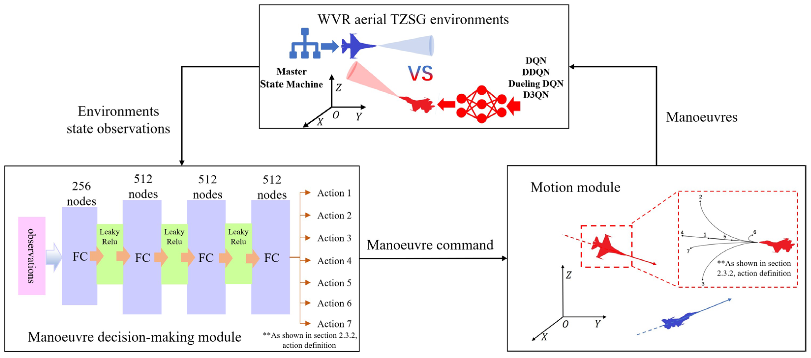
4.1. Experimental Framework

This study investigates a two-player zero-sum game scenario involving agents operating in three-dimensional space. Under given environmental conditions and initial parameters, the controlled agents autonomously formulate strategies based on the situational awareness of both players. The goal is to gain an advantage over the opposing agent and effectively defeat the opponent to achieve victory. Manoeuvre decision making is assisted by DRL algorithms specifically tailored for aerial combat. Experiments compare different algorithms, including DQN, DDQN, Dueling DQN, and D3QN, all using fully connected (FC) neural networks to ensure consistent performance.
As shown in Figure 6, the game process consists of three main modules: environmental interaction, manoeuvre decision, and motion. The environment interaction module provides the gaming environment and observation data. The manoeuvre decision module uses DRL to generate manoeuvre control variables, which the motion module executes. The motion module updates position and attitude through agent motion equations, interacts with the opposing agent, and feeds updated situational information back to the manoeuvre decision module. This iterative process optimises the agent’s manoeuvring strategy, achieving effective and rapid victory in the game.

4.2. Experimental Preparation

4.2.1. Experimental Hardware Preparation

The experimental hardware is Microsoft Windows 11 Flagship 64-bit operating system CPU Inter [email protected] GHz, 32 GB of RAM, GPU RTX4080.

4.2.2. Experimental Software Preparation

The experimental software is the simulation environment is all based on Python3.9.16 language writing, using Pycharm Professional 2023.1.2 and the Anaconda3 platform; the deep reinforcement learning environment uses Pytorch2.1.0 and cuda12.1.

4.2.3. Simulation Experiment Scene Setting

As shown in Figure 6, agent 1 selects actions to execute using DRL algorithms, while agent 2, acting as the opponent, determines its actions based on the master state machine. In the 1v1 autonomous WVR air TZSG scenario, our side starts at a disadvantage, positioned in the enemy aircraft’s advantageous area, as illustrated in Figure 7. Throughout the training, both sides’ positions are fixed and initialised in 3D space, consistently maintaining the depicted posture. Our manoeuvre selection employs a deep reinforcement learning algorithm with a discrete action space (refer to Section 4.3), while the enemy uses an expert system optimised for air combat superiority.
To update the WVR air combat simulation parameters, set the WVR action update cycle to 100 Hz and the air combat decision cycle to 1 Hz. The initial conditions for the Red and Blue agents are as follows in Table 1.
In a zero-sum aerial combat scenario, both the red and blue factions engage in a single episode, with 1000 iterations of combat ensuing. Following this, neural network learning ceases, and both sides utilise network-derived values for decision making in manoeuvring. The blue faction employs state machine-based manoeuvre execution, while the red faction utilises a deep neural network for action selection. The initial aerial combat configuration is depicted in Figure 8. As a control experiment, the strategy of agent (b) remains constant, while agent (r) employs deep reinforcement learning for action selection.

4.2.4. Hyperparameter Settings for Each Algorithm

The hyperparameters used by each of our agents when performing algorithm training are shown below in Table 2.

4.2.5. Algorithm Convergence Criterion

The convergence criteria for the algorithm in this experiment adhere to two widely recognised methods in the academic field of deep reinforcement learning (DRL), as detailed below:
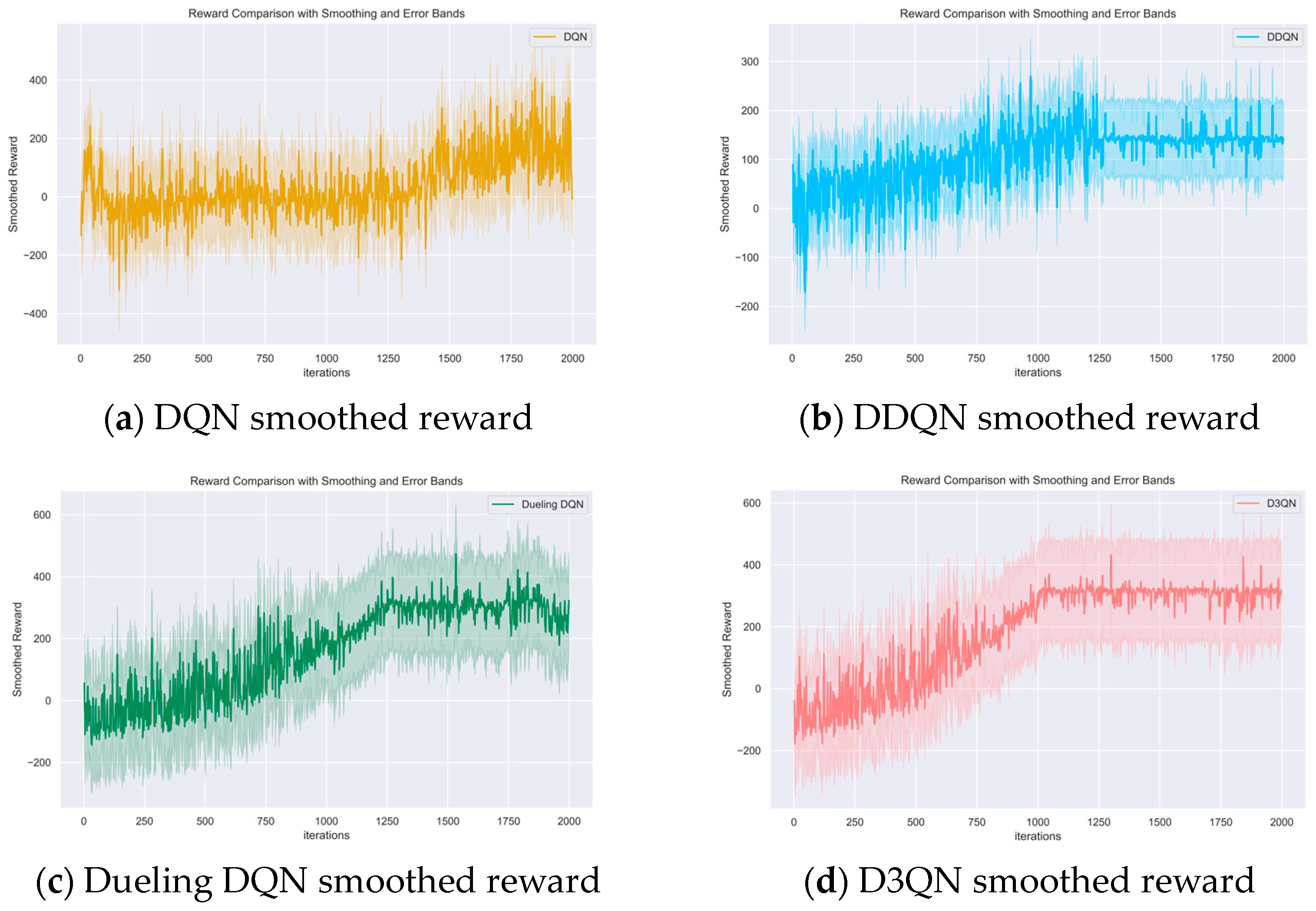
  • Stability of Evaluation Metrics: During training, evaluation metrics gradually stabilise and reach a certain level, indicating that the model’s performance tends to be stable. In this experiment, the primary evaluation metric of interest is the cumulative reward. By plotting the change curve of the cumulative reward over time during training, we can observe the stabilisation of the evaluation metric.
  • No Significant Performance Improvement: Within a certain period, if the model’s performance no longer shows significant improvement, it suggests that further training does not yield noticeable changes in performance metrics. In this experiment, we use the adversarial win rate of the trained model as the performance metric. By setting several predefined training intervals (iterations) and observing the changes in performance metrics during these intervals, we can conclude that the model has converged if there is no significant improvement in performance.

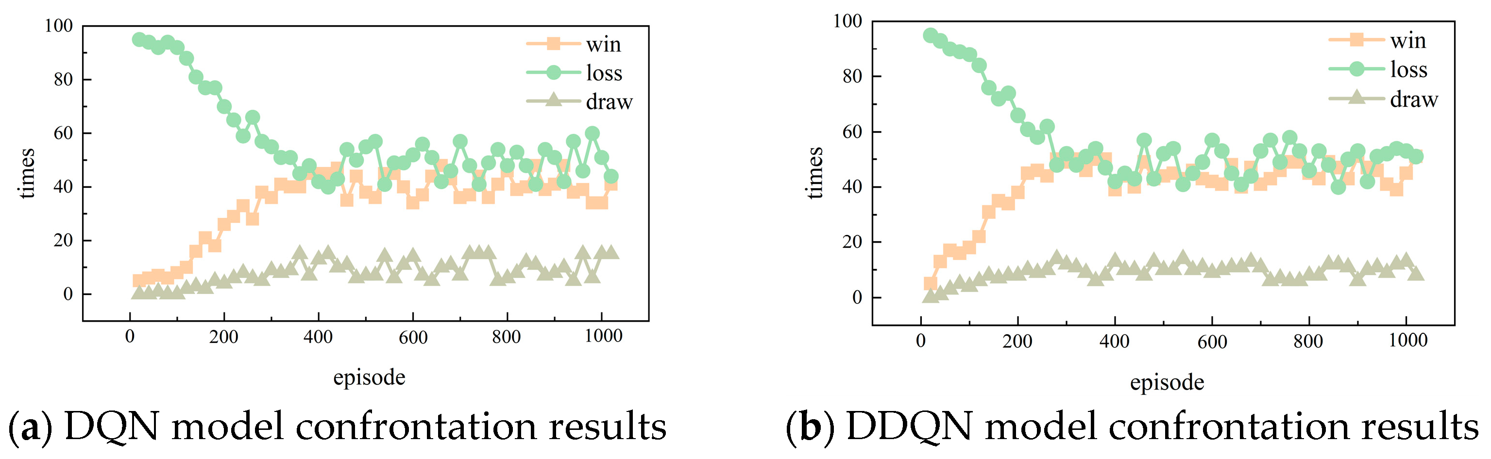
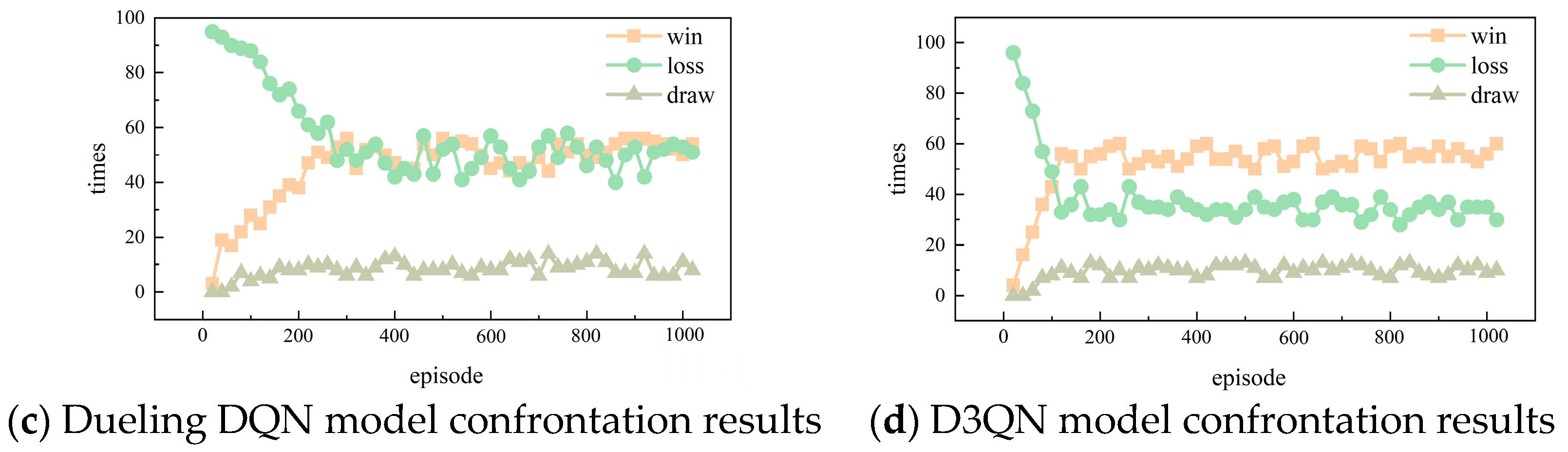
4.3. Experimental Results and Analyses

Four types of discrete action-based deep reinforcement learning (DRL) algorithms, namely DQN, DDQN, Dueling DQN, and D3QN, were trained based on the same environment, identical initial conditions, and partially shared network hyperparameters. The reward curves of the agents during the training process are depicted in Figure 8a–e.
Figure 8. The training results of the deep reinforcement learning (DRL) model.
Mathematics 12 02160 g008aMathematics 12 02160 g008b
From the above figure, it can be seen that all algorithms can have more frequent final round rewards of 200+ or more in large rounds of training, which means that the blue side controlled by the DRL algorithm can beat the red side of the expert system based on the dominance function more consistently in training. Compared to the DQN, shown in Figure 8a, algorithm, DDQN, Dueling DQN, and D3QN, shown in Figure 8b–d, all show superiority in convergence, where D3QN, shown in Figure 8d, has stronger convergence rates, with +100 final step rewards occurring much more frequently than −100 rewards in large rounds of training. The agent is trained due to exploration, so winning or losing a game during training does not indicate the algorithm’s performance. Therefore, it is necessary to conduct multiple rounds of random confrontation between the trained deep network model and the red expert system alone and evaluate its performance. In this experiment, each agent interacts with the environment for 1000 episodes under the control of the same DRL algorithm, with an average of 23,000 steps of agent decision making per episode and 23,000,000 interactions between the agent and the environment. In this paper, the agent will save the current neural network every 20 episodes, in the performance test, each DRL algorithm saved the neural network model by the time sequence was tested with the red side of the random initialisation of 100 battles, and the experimental results obtained are shown in Figure 9a–d
In Figure 9a, the average win rate of the DQN algorithm is about 40% and the wins do not increase significantly at about the 400th episode, which can be regarded as the convergence of the algorithm. In Figure 9b, the average win rate of the DDQN algorithm is about 43% and the algorithm converges at about the 300th episode. In Figure 9c, the Dueling DQN algorithm has an average win rate of about 45% and converges at about the 300th episode. In Figure 9d, the D3QN algorithm has an average win rate of about 52%, and the algorithm converges at about the 180th episode. From the above, the D3QN algorithm shows strong performance in the WVR air two zero-sum game scenario.
Under the same hardware conditions, training environment, and initial state, this experiment statistically analyses the training time of intelligent control algorithms for air combat manoeuvring decisions within a visual range, considering differences in algorithm scale and complexity. The time taken to reach the 1000th training iteration was recorded for each algorithm, as shown in Figure 10.
In the comprehensive above experiments, the DQN algorithm can achieve effective decision making of air manoeuvre strategy and higher efficiency, but its performance is more limited. The DDQN algorithm’s performance has improved, but efficiency has been reduced. Dueling the DQN algorithm and DDQN algorithm performance is similar to that of the DDQN algorithm; efficiency has been reduced slightly. The D3QN algorithm, combining the DDQN and Dueling DQN, has greatly improved performance and convergence, but training efficiency has been reduced.
In addition, all the above four algorithms learn to combine basic technical movements to form tactical manoeuvres in the training process to obtain tactical advantages. Figure 11 shows some screenshots of the simulation environment. The explanation of the manoeuvre can be found in the Glossary.

5. Conclusions

This paper begins by examining the characteristics of within-visual range (WVR) aerial two-player zero-sum games (TZSGs) and establishes a training mechanism for AI algorithms in this context. A reward-shaping method based on the advantage function is designed to address the issue of sparse rewards in WVR aerial TZSG. A benchmark deep reinforcement learning (DRL) algorithm that effectively handles discrete action spaces is selected. The hardware and hyperparameters are standardised, and algorithm training is conducted in an identical environment. Performance validation experiments, decoupled from the algorithm training, are designed to test and analyse the performance of the selected benchmark DRL algorithm. The results indicate that DRL can effectively handle manoeuvring decision problems in WVR aerial TZSG. However, due to the limitations of the benchmark DRL algorithm, there is room for improvement in decision-making performance and accuracy through modifications and adaptations of the DRL algorithm itself. Discussing the limitations of the current approach and potential future work would strengthen the paper’s conclusion.

Author Contributions

Conceptualization, L.R.; Methodology, B.L. and L.R.; Software, B.L. and H.X.; Validation, S.H. and W.W.; Formal analysis, B.L., S.H., W.W. and H.X.; Investigation, B.L. and S.H.; Resources, B.L. and X.Z.; Data curation, B.L., S.H. and W.W.; Writing—original draft, B.L.; Writing—review & editing, B.L. and L.R.; Visualization, H.X.; Supervision, L.R. and X.Z.; Project administration, L.R. and H.X.; Funding acquisition, L.R. and X.Z. All authors have read and agreed to the published version of the manuscript.

Funding

This research received no external funding.

Data Availability Statement

The original contributions presented in the study are included in the article, further inquiries can be directed to the corresponding author.

Conflicts of Interest

The authors declare no conflict of interest.

Glossary

-
Two-player zero-sum games (TZSGs): A model in game theory where the total gains and losses between two participants (players) sum to zero. In other words, one player’s gain equals the other player’s loss. This game model is frequently employed to describe decision-making problems in adversarial environments.
-
Witness Visual Range (WVR): A term used to describe a distance within which objects or targets can be seen with the naked eye. The typical WVR distance can vary depending on visibility conditions, but it is generally up to about 5 nautical miles (approximately 9.3 kilometres or 5.75 miles).
-
Unmanned Aerial Systems (UASs): A term referring to aircraft systems without a human pilot on board, which are controlled remotely or autonomously.
-
Capture zone: A conical spatial area in the heading direction of an aerial agent, defined by a maximum angle and distance, used to represent the agent’s effective capture range.
-
Dominant region: A spatial area that exerts the most influence or control in a given context due to its significant characteristics or activities.
-
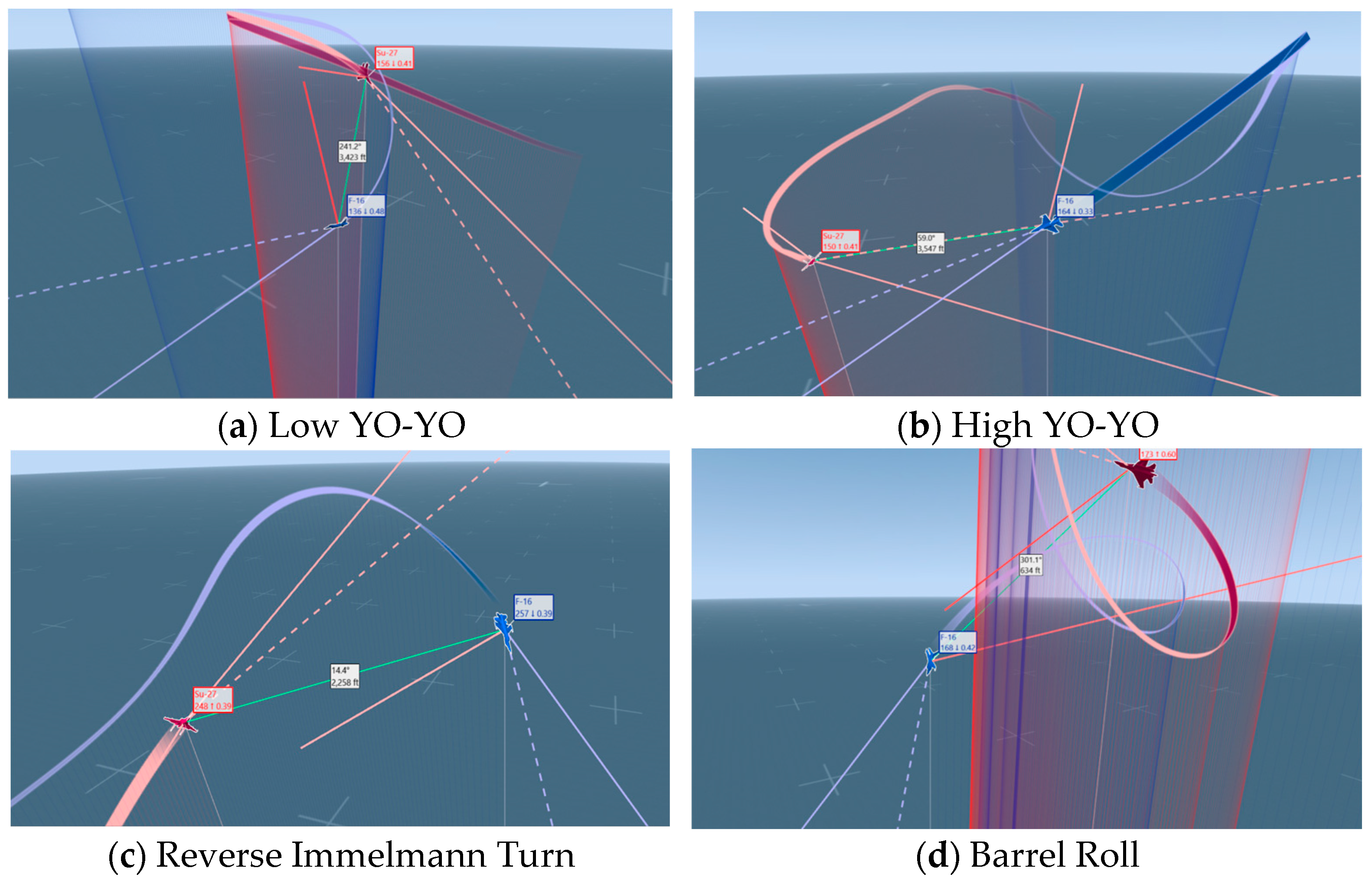
Low YO-YO: The described aerial manoeuvre involves the aircraft pulling up to climb, rolling toward the opponent’s horizontal turn, and inverting. The pilot then pulls up again to position the aircraft towards the enemy. This manoeuvre trades speed for altitude. Thus, it is a lag pursuit manoeuvre, which increases the distance between you and the enemy aircraft.
-
High YO-YO: The described aerial manoeuvre involves the aircraft pushing down to descend, rolling toward the opponent’s horizontal turn, and then pulling up to position the aircraft towards the enemy. This manoeuvre trades altitude for speed. Thus, it is a lead pursuit manoeuvre, which decreases the distance between you and the enemy aircraft.
-
Reverse Immelmann Turn: This is the aerial combat manoeuvre described where a fighter aircraft dives to gain speed, half-rolls to invert, then pulls up into a steep climb and levels out at a higher altitude in the opposite direction. This manoeuvre aids in quickly changing direction and altitude for offensive or defensive advantage.
-
Barrel Roll: The described aerial manoeuvre where an aircraft rotates 360 degrees along its longitudinal axis while following a helical path. It involves pulling back on the stick to pitch up, rolling during the climb, inverting at the top, and completing the roll to return upright. This manoeuvre is used in aerobatics and combat for evasion or positioning.

References

  1. Han, R.; Chen, H.; Liu, Q.; Huang, J. Research on Autonomous Air Combat Maneuver Decision Making Based on Reward Shaping and D3QN. In Proceedings of the 2021 China Automation Conference, Beijing, China, 22–24 October 2021; Chinese Society of Automation: Beijing, China, 2021; pp. 687–693. [Google Scholar]
  2. Ernest, N.; Carroll, D.; Schumacher, C.; Clark, M.; Cohen, K.; Lee, G. Genetic fuzzy based artificial intelligence for unmanned combat aerial vehicle control in simulated air combat missions. J. Def. Manag. 2016, 6, 2167-0374. [Google Scholar] [CrossRef]
  3. Karimi, I.; Pourtakdoust, S.H. Optimal maneuver-based motion planning over terrain and threats using a dynamic hybrid PSO algorithm. Aerospaceence Technol. 2013, 26, 60–71. [Google Scholar] [CrossRef]
  4. Wang, Z.; Li, H.; Wu, H. Improving maneuver strategy in air combat by alternate freeze games with a deep reinforcement learning algorithm. Math. Probl. Eng. 2020, 20, 7180639. [Google Scholar] [CrossRef]
  5. Dong, Y.; Ai, J.; Liu, J. Guidance and control for own aircraft in the autonomous air combat: A historical review and future prospects. Proc. Inst. Mech. Eng. 2019, 233, 5943–5991. [Google Scholar] [CrossRef]
  6. Fu, L.; Wang, X.G. Research on close air combat modelling of differential games for unmanned combat air vehicles. Acta Armamentarii 2012, 33, 1210–1216. (In Chinese) [Google Scholar]
  7. Xie, J. Differential Game Theory for Multi UAV Pursuit Maneuver Technology Based on Collaborative Research. Master’s Thesis, Harbin Institute of Technology, Harbin, China, 2015. (In Chinese). [Google Scholar]
  8. Qian, W.Q.; Che, J.; He, K.F. Air combat decision method based on game-matrix approach. In Proceedings of the 2nd China Conference on Command and Control, Beijing, China, 4–5 August 2014; Chinese Institute of Command and Control: Beijing, China, 2014; pp. 408–412. (In Chinese). [Google Scholar]
  9. Xu, G.; Lu, C.; Wang, G.; Xie, Y. Research on autonomous maneuver decision-making for UCAV air combat based on double matrix countermeasures. Ship Electron. Eng. 2017, 37, 24–28+39. [Google Scholar]
  10. Bullock, H.E. ACE: The Airborne Combat Expert Systems: An Exposition in Two Parts: ADA170461; Defence Technical Information Center: Fort Belvoir, VA, USA, 1986. [Google Scholar]
  11. Chin, H.H. Knowledge-based system of supermaneuver selection for pilot aiding. J. Aircr. 1989, 26, 1111–1117. [Google Scholar] [CrossRef]
  12. Wei, Q.; Zhou, D.Y. Research on UCAV’s intelligent decision-making system based on expert system. Fire Control Command Control 2007, 32, 5–7. (In Chinese) [Google Scholar]
  13. Wang, R.P.; Gao, Z.H. Research on decision system in air combat simulation using maneuver library. Flight Dyn. 2009, 27, 72–75+79. (In Chinese) [Google Scholar]
  14. Virtanen, K.; Ehtamo, H.; Raivio, T.; Hamalainen, R.P. VIATO-visual interactive aircraft trajectory optimization. IEEE Trans. Syst. Man Cybern. Part C Appl. Rev. 1999, 29, 409–421. [Google Scholar] [CrossRef]
  15. Soltanifar, M. A new interval for ranking alternatives in multi attribute decision making problems. J. Appl. Res. Ind. Eng. 2024, 11, 37–56. [Google Scholar]
  16. Farajpour Khanaposhtani, G. A new multi-attribute decision-making method for interval data using support vector machine. Big Data Comput. Vis. 2023, 3, 137–145. [Google Scholar]
  17. Smail, J.; Rodzi, Z.; Hashim, H.; Sulaiman, N.H.; Al-Sharqi, F.; Al-Quran, A.; Ahmad, A.G. Enhancing decision accuracy in dematel using bonferroni mean aggregation under pythagorean neutrosophic environment. J. Fuzzy Ext. Appl. 2023, 4, 281–298. [Google Scholar] [CrossRef]
  18. Hosseini Nogourani, S.; Soltani, I.; Karbasian, M. An Integrated Model for Decision-making under Uncertainty and Risk to Select Appropriate Strategy for a Company. J. Appl. Res. Ind. Eng. 2014, 1, 136–147. [Google Scholar]
  19. Sun, C.; Zhao, H.; Wang, Y.; Zhou, H.; Han, J. UCAV Autonomic maneuver decision- making method based on reinforcement learning. Fire Control Command Control 2019, 44, 142–149. [Google Scholar]
  20. He, L.; Aouf, N.; Whidborne, J.F.; Song, B. Deep reinforcement learning based local planner for UAV obstacle avoidance using demonstration data. arXiv 2020, arXiv:2008.02521. [Google Scholar]
  21. Ma, W. Research on Air Combat Game Decision Based on Deep Reinforcement Learning. Master’s. Thesis, Sichuan University, Chengdu, China, 2021. (In Chinese). [Google Scholar]
  22. Zhou, P.; Huang, J.T.; Zhang, S.; Liu, G.; Shu, B.; Tang, J. Research on UAV intelligent air combat decision and simulation based on deep reinforcement learning. Acta Aeronaut. Astronaut. Sin. 2022, 4, 1–16. Available online: http://kns.cnki.net/kcms/detail/11.1929.v.20220126.1120.014.html (accessed on 18 May 2022). (In Chinese).
  23. Zhang, H.P.; Huang, C.Q.; Xuan, Y.B.; Tang, S. Maneuver decision of autonomous air combat of unmanned combat aerial vehicle based on deep neural network. Acta Armamentarii 2020, 41, 1613–1622. (In Chinese) [Google Scholar]
  24. Pan, Y.; Zhang, K.; Yang, H. Intelligent decision-making method of dual network for autonomous combat maneuvers of warplanes. J. Harbin Inst. Technol. 2019, 51, 144–151. [Google Scholar]
  25. Liu, P.; Ma, Y. A deep reinforcement learning based intelligent decision method for UCAV air combat. In Modelling, Design and Simulation of Systems, Proceedings of the 17th Asia Simulation Conference, AsiaSim 2017, Melaka, Malaysia, 27–29 August 2017; Springer: Singapore, 2017; pp. 274–286. [Google Scholar]
  26. Zhang, Q.; Yang, R.; Yu, L.; Zhang, T.; Zuo, J. BVRair combat maneuvering decision by using Q-network reinforcement learning. J. Air Force Eng. Univ. (Nat. Sci. Ed.) 2018, 19, 8–14. (In Chinese) [Google Scholar]
  27. Kurniawan, B.; Vamplew, P.; Papasimeon, M.; Dazeley, R.; Foale, C. An empirical study of reward structures for actor-critic reinforcement learning in air combat maneuvering simulation. In Advances in Artificial Intelligence; Springer International Publishing: Cham, Switzerland, 2019; pp. 54–65. [Google Scholar]
  28. Yang, Q.; Zhu, Y.; Zhang, J.; Qiao, S.; Liu, J. UAV air combat autonomous maneuver decision based on DDPG algorithm. In Proceedings of the 2019 IEEE 15th International Conference on Control, Edinburgh, UK, 16–19 July 2019. [Google Scholar]
  29. Yang, Q.; Zhang, J.; Shi, G.; Hu, J.; Wu, Y. Maneuver decision of UAV in short-range air combat based on deep reinforcement learning. IEEE Access 2019, 8, 363–378. [Google Scholar] [CrossRef]
  30. Zhou, K.; Wei, R.; Zhang, Q.; Xu, Z. Learning system for air combat decision inspired by cognitive mechanisms of the brain. IEEE Access 2020, 8, 8129–8144. [Google Scholar] [CrossRef]
  31. Zhang, L.; Wei, R.; Li, X. Autonomous tactical decision-making of UCAVs in air combat. Control 2012, 19, 92–96. [Google Scholar]
  32. Ng, A.Y.; Harada, D.; Russell, S. Policy invariance under reward transformations: Theory and application to reward shaping. In Proceedings of the 16th International Conference on Machine Learning, Bled, Slovenia, 27–30 June 1999; pp. 278–287. [Google Scholar]
  33. Kober, J.; Bagnell, J.A.; Peters, J. Reinforcement learning in robotics: A survey. Int. J. Robot. Res. 2013, 32, 1238–1274. [Google Scholar] [CrossRef]
  34. Goodfellow, I.; Bengio, Y. Deep Learning; MIT Press: Cambridge, MA, USA, 2017. [Google Scholar]
  35. Sutton, R.; Barto, A. Reinforcement Learning; MIT Press: Cambridge, MA, USA, 2018. [Google Scholar]
  36. Mnih, V.; Kavukcuoglu, K.; Silver, D.; Rusu, A.A.; Veness, J.; Bellemare, M.G.; Graves, A.; Riedmiller, M.; Fidjeland, A.K.; Ostrovski, G.; et al. Human-level control through deep reinforcement learning. Nature 2015, 518, 529–533. [Google Scholar] [CrossRef] [PubMed]
  37. Silva, B.P.; Ferreira, R.A.; Gomes, S.C.; Calado, F.A.; Andrade, R.M.; Porto, M.P. On-rail solution for autonomous inspections in electrical substations. Infrared Phys. Technol. 2018, 90, 53–58. [Google Scholar] [CrossRef]
  38. Van Hasselt, H.; Guez, A.; Silver, D. Deep reinforcement learning with double Q-Learning. Natl. Conf. Artif. Intell. Proc. AAAI Conf. Artif. Intell. 2016, 30, 2094–2100. [Google Scholar] [CrossRef]
  39. Chou, C.-H. Machine Learning; Tsinghua University Press: Beijing, China, 2016. [Google Scholar]
  40. Harrington, P. Machine Learning in Action; People’s Posts and Telecommunications Press: Beijing, China, 2013. [Google Scholar]
  41. Duan, Y.; Xu, X.; Xu, S. Research on multi-robot collaboration strategy based on multi-intelligent body reinforcement learning. Syst. Eng. Theory Pract. 2014, 34, 1305–1310. [Google Scholar]
  42. Zhang, H.C.; Zhao, K.; Li, L.M.; Liu, H. Power system restoration overvoltage prediction based on multilayer artificial neural network. Smart Power 2018, 46, 67–73+88. [Google Scholar]
  43. Wang, Z.Y.; Schaul, T.; Hessel, M.; Hasselt, H.; Lanctot, M.; Freitas, N. Dueling network architectures for deep reinforcement learning. In Proceedings of the 33rd International Conference on Machine Learning, New York, NY, USA, 20–22 June 2016; ACM: New York, NY, USA, 2016; pp. 1995–2003. [Google Scholar]
Figure 1. Two aerial agents WVR TZSG model.
Mathematics 12 02160 g001
Figure 2. Schematic of the capture zone.
Mathematics 12 02160 g002
Figure 3. Basic manoeuvres.
Mathematics 12 02160 g003
Figure 4. Dominant region schematic diagram.
Mathematics 12 02160 g004
Figure 5. Reinforcement learning algorithm framework for autonomous manoeuvre decision making in aerial TZSG agent games.
Mathematics 12 02160 g005
Figure 6. Simulation module interaction process.
Mathematics 12 02160 g006
Figure 7. Initial state of the environment.
Mathematics 12 02160 g007
Figure 9. Red–blue confrontation training curve.
Mathematics 12 02160 g009aMathematics 12 02160 g009b
Figure 10. Statistics of the time to reach the maximum number of training rounds for the 4 DRL algorithms.
Mathematics 12 02160 g010
Figure 11. Screenshot of the simulation training/experiment environment.
Mathematics 12 02160 g011
Table 1. Agent initial setting.
ParameterAgent (r)Agent (b)
Spatial coordinates c r = 1997.48 ,   0.04 , 6000.19 c b = 0.04 ,   2.50 , 7000.19
Trajectory inclination γ r = 0 γ b = 0
Trajectory declination ψ r = 0 ψ b = 270
Velocity magnitude v r = 180   m / s v b = 200   m / s
Table 2. List of hyperparameters of agent algorithm.
Hyper Parameterisation(Be) Worth
random seed1
Maximum number of steps in a round50,000
training wheels1000
Number of hidden layer nodes256
Update Batch512
optimiserAdam
Experience pool capacity1,000,000
Number of hidden layer nodes128
Frequency of target network updates1000 steps.
learning rate0.001
probability of exploration0.9
Incentive Discount Factor0.95
Disclaimer/Publisher’s Note: The statements, opinions and data contained in all publications are solely those of the individual author(s) and contributor(s) and not of MDPI and/or the editor(s). MDPI and/or the editor(s) disclaim responsibility for any injury to people or property resulting from any ideas, methods, instructions or products referred to in the content.

