Abstract
This study introduces a novel method for classifying sets of images, called Riemannian geodesic discriminant analysis–minimum Riemannian mean distance (RGDA-MRMD). This method first converts image data into symmetric positive definite (SPD) matrices, which capture important features related to the variability within the data. These SPD matrices are then mapped onto simpler, flat spaces (tangent spaces) using a mathematical tool called the logarithm operator, which helps to reduce their complexity and dimensionality. Subsequently, regularized local Fisher discriminant analysis (RLFDA) is employed to refine these simplified data points on the tangent plane, focusing on local data structures to optimize the distances between the points and prevent overfitting. The optimized points are then transformed back into a complex, curved space (SPD manifold) using the exponential operator to enhance robustness. Finally, classification is performed using the minimum Riemannian mean distance (MRMD) algorithm, which assigns each data point to the class with the closest mean in the Riemannian space. Through experiments on the ETH-80 (Eidgenössische Technische Hochschule Zürich-80 object category), AFEW (acted facial expressions in the wild), and FPHA (first-person hand action) datasets, the proposed method demonstrates superior performance, with accuracy scores of 97.50%, 37.27%, and 88.47%, respectively. It outperforms all the comparison methods, effectively preserving the unique topological structure of the SPD matrices and significantly boosting image set classification accuracy.
Keywords:
image set classification; Riemannian manifold; tangent space; symmetric positive definite matrices; regularized local Fisher discriminant analysis; minimum Riemannian mean distance MSC:
68T10; 68U10; 94A12; 15B48
1. Introduction
In the digital age, visual (image set) classification has emerged as a significant area of research within the fields of computer vision and machine learning [1,2,3]. Unlike traditional single-image classification, image set classification deals with a collection of images that together represent an object or scene. This approach has shown unique advantages for various applications, such as facial recognition [4], fault diagnosis [5], and medical image analysis [6].
One major challenge to image set classification is effectively processing and representing high-dimensional image data. Traditional methods, such as directly flattening images into vectors, often lead to the curse of dimensionality and the loss of information [7,8]. The curse of dimensionality refers to the various phenomena that arise when analyzing and organizing data in high-dimensional spaces. As the dimensionality increases, the volume of the space increases exponentially, making data analysis computationally challenging and often leading to sparse and less informative data distributions.
In contrast, deep learning methods, particularly those based on convolutional neural networks (CNNs), have demonstrated superior performance in many visual tasks. These methods achieve powerful classification capabilities by automatically learning the hierarchical feature representations of data [9,10]. However, deep learning models typically require large amounts of labeled data for training and lack an intuitive exploitation and interpretation of the intrinsic geometric structure of image sets. Additionally, when dealing with highly nonlinear manifold data, traditional CNNs may fail to capture all the significant features of the data, leading to degraded performance.
To overcome these issues, manifold learning approaches have been proposed to exploit the geometric structure within image sets. These methods assume that the data points (such as images) lie on an underlying low-dimensional manifold, and by learning the structure of this manifold, more robust and informative latent representations can be obtained [11,12].
The recent manifold learning-based methods for image set classification can be broadly categorized into three types: manifold sparse representation methods [13,14,15], Riemannian metric learning methods [16,17,18], and manifold deep learning methods [19,20]. Manifold sparse representation methods leverage the principle of sparse coding, which can effectively utilize the sparsity nature of image data. However, they heavily rely on the computation of a logarithmic map, leading to high computational costs. Moreover, these algorithms are specifically designed for manifold structures, resulting in poor generalizability. Riemannian metric learning methods enhance classification performance by learning an optimal metric on the Riemannian manifold, which improves the measure of the distances between data points. Yet, they depend on an optimization process, which may require substantial computational resources. Manifold deep learning methods are capable of automatically learning the complex nonlinear structures of data, but they need extensive labeled data for training. Additionally, the internal mechanisms of these models are difficult to interpret.
The focus of this paper is predominantly on the methods related to Riemannian metric learning, emphasizing the significance of maintaining positive definiteness within the Riemannian metrics, a fundamental element of these techniques. Presently, two prevalent strategies exist for analyzing symmetric positive definite (SPD) matrices to facilitate classification tasks. The first strategy involves embedding the data into a high-dimensional Hilbert space via positive definite Riemannian kernels [21,22]. However, this method of feature transformation may compromise the intrinsic Riemannian geometric structure of the original data manifold. Moreover, the computational burden of calculating the kernel matrices escalates exponentially with an increase in data size. Alternatively, the second strategy seeks to project the Riemannian manifold onto a tangent space (which can be viewed as a Euclidean space), thereby enabling the learning of Euclidean feature representations or the reduction in dimensions directly from the original Riemannian manifold-valued data [23,24].
In this paper, we present a novel and effective methodology for classifying image sets, called Riemannian geodesic discriminant analysis–minimum Riemannian mean distance (RGDA-MRMD) method, wherein SPD matrices are utilized to represent the image sets as covariance matrices, which are subsequently projected onto the tangent space. This is followed by dimensionality reduction and feature extraction using regularized local Fisher discriminant analysis (RLFDA), and then reconstructing the projection plane based on the geodesic filtering algorithm, mapping the data back onto the Riemannian manifold space for the final classification of the image sets.
The choice of SPD matrices arises from their ability to faithfully represent covariance structures within image sets, which is crucial for capturing variances and relationships across multiple images. This representation is pivotal for tasks in which understanding intra-class variations and inter-class distinctions are paramount.
RLFDA is chosen for its dual advantages of incorporating local data structures and regularization within the SPD manifold. Regularization enhances model robustness by preventing overfitting, which is particularly beneficial when the labeled data are limited. Moreover, RLFDA’s emphasis on local characteristics ensures that the discriminant analysis accounts for the proximity of the data points within their respective classes within the context of the SPD matrices, thus refining the classification boundaries.
Specifically, to circumvent the distortion issue of Riemannian features in the reproducing kernel Hilbert space (RKHS), we first project the covariance feature matrices from the Riemannian manifold onto the tangent space, centered at the Riemannian mean via the logarithmic map. This not only reduces the dimensionality and complexity of the SPD matrices, but also facilitates further feature extraction within this planar space using RLFDA, segregating the points based on their maximum inter-class distance and minimum intra-class distance to yield an approximate projection geodesic. Unlike traditional FDA, RLFDA enhances classification performance by incorporating local data structures and regularization, thereby focusing more on the local neighborhood characteristics of the sample points and improving robustness. Subsequently, the projection plane of RLFDA is reconstructed using a geodesic filtering algorithm, establishing a separable tangent plane. Through the exponential map, the separable covariance feature data on this tangent plane are remapped back onto the Riemannian manifold space. Finally, to preserve the unique topological structure of the SPD matrices, such as their positive definiteness, we employ the MRMD algorithm to classify the data points on the Riemannian manifold, thereby improving the accuracy and effectiveness of the image set classification. The experiments we conduct on three datasets demonstrate that our algorithm significantly outperforms other state-of-the-art methods, showcasing remarkable improvements in classification outcomes.
The key goals of our study can be summarized as follows:
Methodological innovation: We introduce RGDA-MRMD, a novel method that integrates Riemannian geometry with discriminant analysis techniques to enhance the classification accuracy of image sets. This involves transforming image set representations into SPD matrices, projecting them onto tangent spaces for dimensionality reduction, and applying discriminant analysis for feature extraction and classification.
Performance evaluation: We evaluate the effectiveness of RGDA-MRMD against the state-of-the-art methods for image set classification tasks across multiple benchmark datasets. It demonstrates significant improvements in classification accuracy and robustness, particularly in scenarios where traditional methods and deep learning approaches face challenges.
Interpretability and robustness: We address the interpretability concerns associated with deep learning models by emphasizing the intuitive exploitation of geometric structures inherent in image sets. We highlight the robustness of RGDA-MRMD for handling complex manifold data and noisy environments, thereby offering insights into its applicability across various domains.
2. Related Work
In recent years, researchers have developed effective Riemannian manifold-based strategies for data modeling, learning, and classification to exploit data’s non-Euclidean properties. These strategies typically model image sets as points on Grassmann or SPD manifolds, diverging from traditional vector space structures. Existing image set classification methods based on Riemannian manifolds can be broadly categorized into manifold sparse representation, Riemannian metric learning, and manifold deep learning methods.
- (1)
- Manifold sparse representation methods:These methods handle data analysis and machine learning by treating the data points as elements on a geometric manifold instead of in Euclidean space.
- (a)
- Intrinsic strategy: This strategy leverages intrinsic manifold properties for sparse coding, such as geodesic distance. For instance, Ertan et al. [25] integrated sparse representation theory and Riemannian geometry into a graph theory segmentation framework, utilizing the Riemannian properties of the directional distribution functions.
- (b)
- Extrinsic strategy: This strategy embeds the manifold into a vector space and performs sparse representation and dictionary learning there. Harandi et al. [13] mapped the Grassmann manifold onto the space of symmetric matrices, demonstrating that the Euclidean distance metric in this symmetric matrix space is equivalent to the geodesic distance in the Grassmann manifold.
- (2)
- Riemannian metric learning:
- (a)
- Kernel-based methods: These techniques involve embedding Riemannian manifolds into a high-dimensional RKHS, behaving like Euclidean space. For instance, Hamm et al. [1] proposed Grassmann Discriminant Analysis (GDA), utilizing Grassmann kernels to define distance metrics between subspaces.
- (b)
- Tangent space-based methods: These methods approximate Riemannian manifolds using tangent spaces, applying traditional metric learning methods within the resulting Euclidean tangent space. Tuzel et al. [24] introduced the LogitBoost algorithm into the SPD manifold, mapping points to the tangent plane centered at the Karcher mean of the Riemannian manifold.
- (3)
- Riemannian metric learning (deep learning methods):These methods represent image set data as points on Riemannian manifolds, utilizing layers similar to “activation” functions in Euclidean space to process the data. For example, Huang et al. [26] proposed a network model based on the SPD manifold, comprising BiMap, ReEig, and LogEig layers. Nguyen et al. [19] designed a deep neural network based on Gaussian embedding of Riemannian manifolds for three-dimensional gesture recognition tasks.
Identified Gaps
While the aforementioned methods have advanced image set classification on Riemannian manifolds, they each have limitations.
Manifold sparse representation methods: These often require high computational resources for sparse coding on manifolds, and may not generalize well across different manifold structures.
Riemannian metric learning methods: These can be computationally intensive due to kernel matrix calculations and may lose the intrinsic geometric structure when embedding into RKHS or approximating with tangent spaces.
Manifold deep learning methods: These depend heavily on large amounts of labeled data and can be difficult to interpret due to their complex architecture.
Our proposed method, RGDA-MRMD, aims to address these gaps by combining the strengths of Riemannian metric learning and robust feature extraction while maintaining computational efficiency and the intrinsic geometric properties of the data. By projecting SPD matrices onto a tangent space for dimensionality reduction and then using RLFDA, our method preserves essential local structures and enhances classification robustness. The final classification is performed in Riemannian space, ensuring the preservation of the topological structure of SPD matrices and improving classification accuracy.
3. Riemannian Geometry Theory
3.1. Subsection
The covariance matrix resides within the realm of SPD matrices, which are endowed with a Riemannian metric, defining a smooth, differentiable Riemannian manifold. This manifold lies within a non-Euclidean space, indicating that the usual Euclidean geometry does not apply. The Riemannian metric can characterize the geometric structure of SPD matrices.
A symmetric matrix space is defined as
A positive definite matrices space is defined as
A SPD matrices space is defined as
Every non-zero vector , when multiplied by a real SPD matrix , yields a positive scalar , highlighting the SPD matrix’s definitive positive nature. The collective domain of these matrices forms a convex cone’s interior within a Euclidean space of dimensions, known as .
3.2. Tangent Space
When endowed with an appropriate Riemannian metric, becomes a Riemannian manifold. This manifold structure allows for the generalization of straight lines in Euclidean space to geodesics on the SPD manifold.
Due to the topological structure of the SPD manifold, it resembles a local Euclidean space globally differentially defined as a Riemannian manifold. At each point C on the Riemannian manifold , the set of all tangent vectors forms a tangent space with a Euclidean structure:
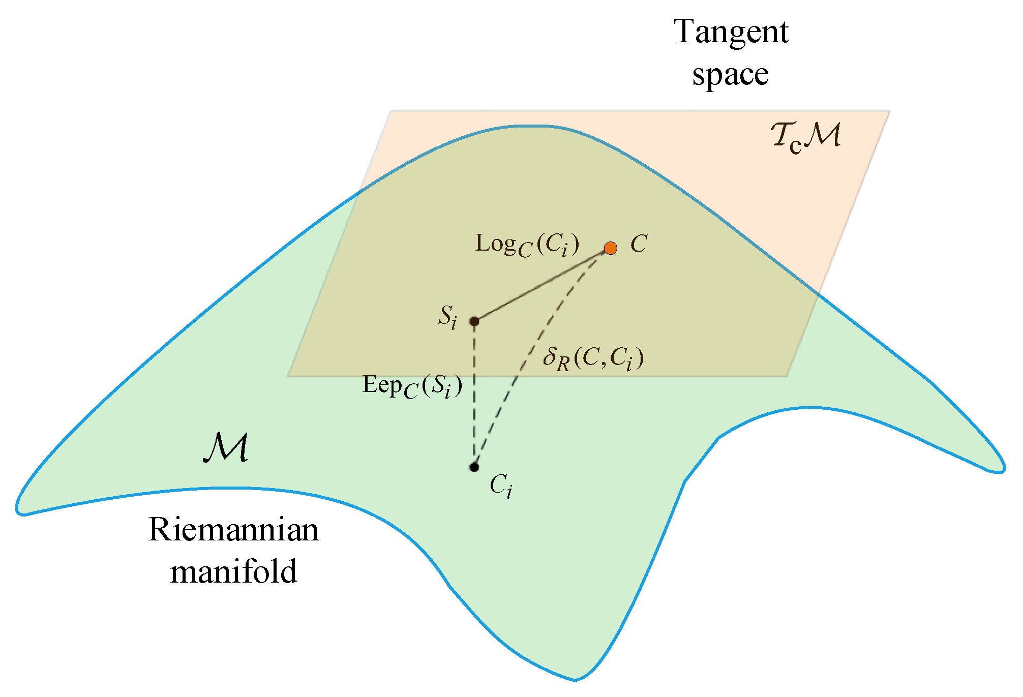
Figure 1 elucidates that the SPD matrices C, are projected onto within the Riemannian manifold , and correspondingly within its tangent space , indicated as . This tangent space embodies a Euclidean framework and exhibits local topological equivalence to the Riemannian manifold.
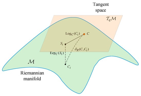
Figure 1.
Illustration of Riemannian manifold along with its associated tangent space . C is located in both the manifold and the tangent space, while resides within the tangent space. The geodesic distance on the manifold measures how far apart C and are within this curved space. Through the tangent point C, and can be related to each other by the logarithm and exponential maps, respectively.
Consider that all the singular vectors of C are encapsulated in the matrix U. The singular values of matrix C, in descending order, are denoted as . Then,
From Figure 1, it can be seen that for any SPD matrices on the Riemannian manifold, the tangent vectors in the tangent space formed by the tangent point C can be represented through logarithmic mapping, . It can be defined as
where the operation represents the matrix logarithm. is defined as the result of taking the logarithm of each diagonal element of the matrix , obtained from the eigenvalue decomposition of a SPD matrix C:
Similarly, for any tangent vectors in the tangent space, the SPD matrices on the Riemannian manifold can be obtained through exponential mapping, . It can be defined as
where the operation represents matrix exponentiation. is the result of exponentiating each diagonal element of matrix C:
The exponential operator maps the SPD matrices from the tangent space onto the Riemannian manifold, while the logarithmic operator is its inverse function.
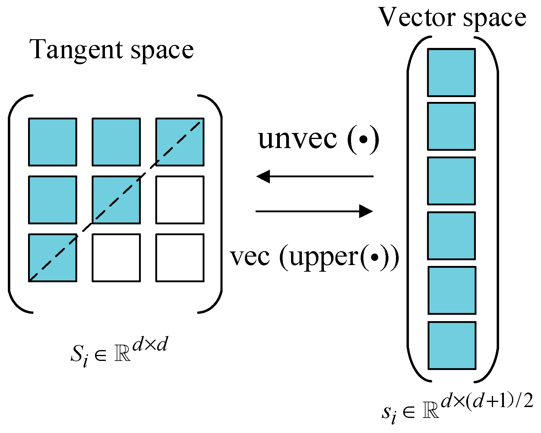
Typically, the Riemannian tangent space belongs to a linear subspace of dimension . Since is a symmetric matrix, the information about the matrix can be represented by the elements in the upper triangle, encompassing all the necessary information. The vector space of the tangent plane at point C on the manifold can be defined as
where the operation denotes the vectorization of the upper-triangular elements of a matrix, doubling the off-diagonal elements, while retaining the diagonal ones unchanged. These operators map the SPD matrices in a tangent space to vectors within a vector space, as illustrated in Figure 2.

Figure 2.
Mapping between SPD matrices in tangent space and vectors in vector space.
In the context of vector spaces, represents the dimensional vector that spans the space. Conversely, the operation is defined as the transformation that reshapes the vectors within a vector space into tangent matrices in a tangent space, . A deeper understanding of Riemannian manifold theory can be seen in [27].
3.3. Riemannian Geodesic Distance
Because of the manifold’s curvature, Euclidean metrics fail to gauge the true distance between SPD matrices and within a Riemannian space. Riemannian geodesic distance steps in to accurately describe the shortest path connecting them, reflecting the manifold’s complex geometry. For SPD matrices and , it can be defined as
where denotes the i-th () singular value of , and denotes the Frobenius norm.
The geodesic on a Riemannian manifold is intimately related to the tangent vectors in the tangent plane space. For each tangent vector in the manifold, there exists a unique geodesic in the Riemannian space corresponding to it. Hence, the geodesic distance between and in a Riemannian manifold can also be expressed as
The Riemannian geodesic distance possesses the following properties:
- (1)
- Non-negativity:
- (2)
- Symmetry:
- (3)
- Inverse invariance:
- (4)
- Affine transformation invariance:where K is any arbitrary nonsingular matrix. This property demonstrates the affine invariance of the geodesic distance between two points on a Riemannian manifold, indicating that the geodesic distance remains unchanged after transformation via mapping.
3.4. Riemannian Geodesic Distance
Since the geodesic distance between the data points and the tangent point is greater, the error in the mapping of Riemannian tangent space tends to be larger. Generally, selecting the Riemannian mean center of the dataset as the tangent point for mapping helps to reduce this error. According to the definition of Euclidean distance, the mean of Euclidean space, which minimizes the distance between the center point of the dataset and the average distance of the dataset, is defined as
where are located in Euclidean space, and aims to flatten a two-dimensional matrix into a one-dimensional vector.
Similarly, according to the definition of Riemannian geodesic distance, in Riemannian space, the point whose Riemannian distance to the dataset is minimized is termed the Riemannian mean center point, defined as
For a local Riemannian manifold, the Riemannian center point is unique, but the Riemannian mean point lacks a unique analytical solution. Iterative approximation, such as Fletcher’s method [28], is often used. It involves projecting the dataset onto the current tangent space centered at the Riemannian mean point. Then, the mean center point in Euclidean space is computed within this tangent space, becoming the new tangent point. Iterations continue until the difference between the mean points falls below a threshold. The tangent point then becomes the Riemannian mean point.
4. RLFDA Algorithm
4.1. Fisher Discriminant Analysis (FDA)
FDA [29] is a supervised dimensionality reduction method. Its main principle is to find the optimal projection direction, where samples of the same class are as close as possible, and samples of different classes are as far apart as possible after projection. Then, based on the position of the unknown class samples after projection in this direction, the class is determined.
Assume labeled samples with corresponding labels , where n denotes the number of samples and c denotes the number of classes.
Let and represent the within-class scatter matrix and between-class scatter matrix, respectively.
where represents the mean value of the samples in class l, represents the mean value of the entire sample set, and represents the number of samples belonging to class l.
Assuming the within-class scatter matrix is full rank, the objective function of FDA can be defined as follows:
where is the projection matrices and denotes the trace of a matrix. g represents the lower projecting dimension, at most dimensions.
FDA aims to maximize the between-class scatter and minimize the within-class scatter, ensuring effective class separation in a low-dimensional space. However, its performance may suffer from non-Gaussian data distributions. The between-class scatter matrix’s rank is at most , allowing for meaningful features. Additionally, FDA overlooks multimodal class distributions and outliers.
4.2. Local Fisher Discriminant Analysis (LFDA)
Let represent the labeled dataset, and represent the entire dataset, where and denote the i-th data point and the corresponding label, c is the number of classes, d is the dimensionality of the original space, n is the total number of labeled data, m is the total number of training samples, and , is the unlabeled dataset.
If is transformed into its projected representation in an r-dimensional subspace using the projection matrix , the projected function can be
Therefore, the LFDA objection function [30] can be defined as follows:
where and denote the within-class scatter matrix and between-class scatter matrix in LFDA, as detailed in [31].
Obviously, the objective of LFDA is to find a projection matrix that maximizes the ratio of to .
4.3. RLFDA
When LFDA lacks sufficient labeled samples for training, it is prone to overfitting. To mitigate this issue, a common approach is to introduce a regularization term related to the unlabeled samples into the objective function.
The objective function of RLFDA is as follows:
where and are two regularization terms associated with the unlabeled data, used to regularize the between-class scatter matrix and within-class scatter matrix, respectively. is the regularization factor.
The regularization term can be introduced based on locality preserving projections (LPP) to achieve the assumption of local spatial consistency [31]. This means that the samples that exhibit high consistency in the original space should also be close to each other in the reduced-dimensional space. After regularization using LPP, the expressions for the between-class scatter and within-class scatter matrices are as follows:
where is an diagonal matrix, and its i-th diagonal element is given by
is an matrix, and its elements are
where is the similarity between and , as defined in the similarity matrix [31]:
where represents the local scaling parameter for :
where represents the k-th nearest neighbor of , and denotes the Euclidean distance.
The parameter γ is determined based on the local scaling parameter approach, where it adapts to the local density of the data. We set γ according to the distance to the k-nearest neighbor, typically chosen from a range of [5, 20]. This choice helps to maintain local consistency while preventing too tight or too loose neighborhood definitions.
We find that setting k = 7 provides a good compromise between capturing sufficient local structure and computational efficiency. For γ, we use the median distance to the seventh nearest neighbor as the scaling factor. Details can be seen in Section 6.7.
Therefore, can be further represented in the following matrix form:
where , and is a diagonal matrix with its i-th diagonal element given by
After regularization using LPP, the matrix expression of the objective function for RLFDA can be changed to
Furthermore, by solving the optimization objective in the form of generalized eigenvalue equations, we can obtain the top generalized eigenvectors corresponding to the largest generalized eigenvalues. These eigenvectors form the optimal projection matrix .
5. Proposed Method
5.1. RGDA-MRMD Algorithm
RGDA is an extension of the RLFDA algorithm tailored for Riemannian manifolds. Its core aim is to boost the separability between classes and diminish intra-class differences, thereby enhancing classification accuracy. The following is a detailed breakdown of the RGDA algorithm, where m is the dimensionality of the manifold representations and n is the image set samples.
- (1)
- SPD representation:
Image dataset transformation: Initially, the image dataset is transformed into SPD matrices, capturing the covariance features of the images.
- (2)
- Map onto SPD manifold:
Riemannian manifold mapping: The SPD matrices are then mapped onto the SPD manifold, representing the data points as elements on a geometric manifold rather than in Euclidean space.
- (3)
- Project onto tangent space:
Logarithm mapping: Using the logarithm operator, the covariance feature points on the SPD manifold are mapped onto tangent spaces centered at Riemannian means.
Vectorization: These points on the tangent spaces are then vectorized to facilitate further analysis.
- (4)
- Employ RLFDA:
RLFDA application: The vectorized data points on the tangent plane are projected using Riemannian local Fisher discriminant analysis (RLFDA). This projection maximizes the between-class distance while minimizing the within-class distance.
Geodesic projection: This process yields an approximate projection of geodesics on the tangent plane, enhancing class separability.
- (5)
- Reconstruct projected geodesics:
Separable tangent plane creation: The projected geodesics plane is reconstructed to craft a separable tangent plane.
Exponential mapping: Leveraging the exponential operator, the separable data points on the tangent plane are mapped back onto the Riemannian manifold space.
- (6)
- Map back onto SPD manifold:
Riemannian space mapping: After reconstruction, the data points are mapped back onto the SPD manifold, maintaining the newly found separability from the tangent space.
- (7)
- Use MRMD algorithm to classify:
MRMD algorithm application: Finally, the classified data points are determined based on the MRMD algorithm.
Class assignment: Each data point is assigned to the class with the closest mean point in the Riemannian space, achieving accurate classification.
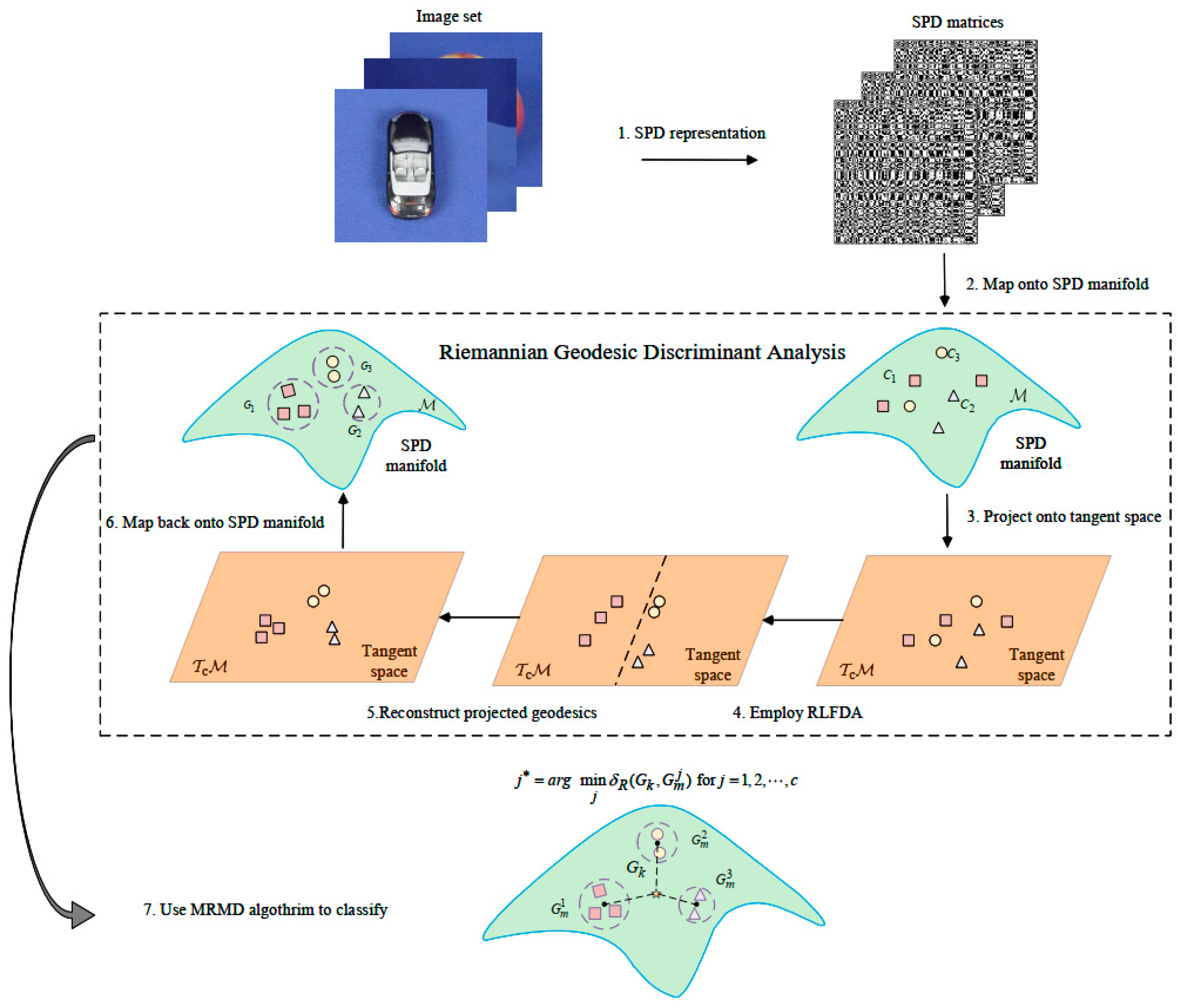
By executing these steps, the RGDA method effectively enhances the separability of class data points on the Riemannian manifold, while simultaneously minimizing intra-class differences. This leads to improved discriminative power and better classification performance. The whole framework is shown in Figure 3.
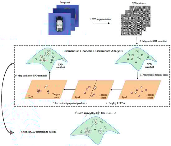
Figure 3.
The proposed RDGA-MRMD framework for image set classification.
5.2. Pseudo Code
Let denote the i-th image set comprising entities, where represents the j-th image sample. For , the covariance matrix can be computed as
where m denotes the mean of . The positive definiteness of can be maintained through the following method:
where denotes identity matrices and is the positive definiteness factor.
Then, the image set can be represented in the SPD manifold as , where N is the total labeled number, , and , with c denoting the number of different classes. For every SPD data point, Ci can be projected onto the tangent plane using Equation (10) to obtain manifold feature vectors .
Next, RLFDA is applied to the feature vectors to obtain a discriminative mapping matrix .
Subsequently, the projected plane needs to be reconstructed. Assuming is the reconstruction matrix, the least squares method is employed as the loss function for the reconstruction matrix:
The optimal solution is
Utilizing the reconstruction matrix for geodesic discriminant analysis on manifold feature vectors, the resulting manifold feature vectors after discrimination are represented as
Furthermore, the new tangent plane data points are remapped back onto the Riemannian space using the exponential operator, yielding
Finally, the MRMD algorithm is utilized for classification. In the training phase, the Riemannian mean center points for each class on the SPD manifold , after undergoing RGDA, are computed. Then, in the testing phase, the geodesic distances between the unknown samples and the Riemannian mean center points of each class are calculated. The class of the nearest mean point, in terms of geodesic distance, is assigned to the unknown sample as its class. That is:
The whole procedure of the proposed method for image set classification can be summarized as Algorithm 1.
| Algorithm 1: RGDA-MRMD Algorithm. |
Input: Original image set , where N is the total labeled number, , and , with c denoting the number of different classes.
|
Training:
|
Testing:
|
| Output: The predicted labels for the test image set, j∗. |
6. Implementation Details and Results
6.1. Image Set Datasets
- ETH80 (Eidgenössische Technische Hochschule Zürich-80 object category) [32]
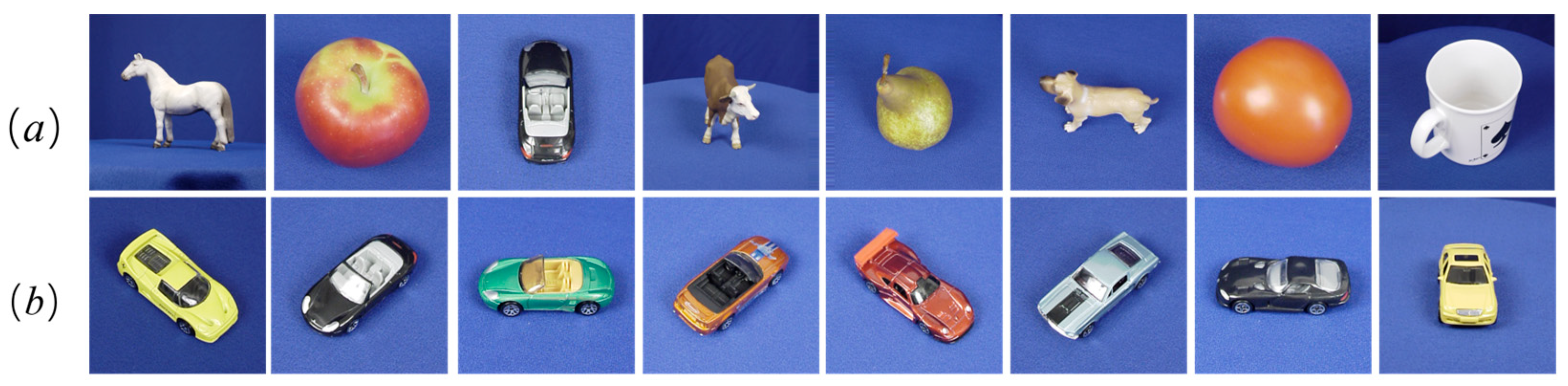
It is composed of eight unique object categories: a cow, cup, horse, dog, potato, car, pear, and apple. Each category encompasses 10 distinct subcategories, with each subcategory forming an image set sample. Furthermore, every image set sample comprises 41 images captured from diverse viewpoints. Select examples of these categories are depicted in Figure 4. Additionally, 80 unlabeled data samples are generated through operations such as rotation, flipping, and noise addition. Five image sets are randomly selected from each class for training, while the remaining sets are used for testing.
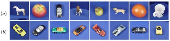
Figure 4.
(a) Examples representing the eight object categories in the ETH-80 dataset. (b) Examples showcasing the diverse classes within a single object category.
- 2.
- Acted facial expression in the wild (AFEW) [33]
It comprises 1345 video segments belonging to seven facial expression types. AFEW consists of close-to-real-world clips extracted from movies, showing characters in various emotional states. The dataset contains sequences of facial expressions categorized into different classes, like anger, sadness, happiness, surprise, disgust, fear, and contempt. To ensure fair experimental comparison, following the criteria in the literature [26], AFEW is initially partitioned into training, validation, and test sets, and the training sets are augmented to 1746. Similarly, an equivalent amount of unlabeled data, obtained through operations such as rotation, flipping, and noise addition, is provided. Some examples are shown in Figure 5.
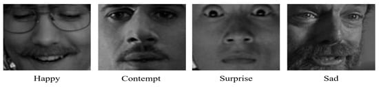
Figure 5.
Sampled facial expression examples from the AFEW dataset.
To ensure fair experimental comparison, the images from the aforementioned two datasets are first converted to grayscale and then resized to dimensions. In this scenario, the i-th video segment (image set) is transformed into a image set matrix, which can be represented as a SPD matrix.
- 3.
- First-person hand action (FPHA) [34]
This dataset is a large-scale benchmark for first-person hand gesture estimation, comprising 1175 action sequences belonging to 45 different gesture categories. These actions are captured by six demonstrators in three different visual scenes. Due to the significant variations in style, movement speed, scale, and viewpoint across the samples in this dataset, the task of first-person gesture recognition presents considerable challenges. Partial examples from this dataset are shown in Figure 6. For consistency in the experimental comparisons, following the guidelines in [35], each frame image is converted into a 63-dimensional vector using the provided 21 hand skeleton points’ 3D coordinates. At this point, the original i-th video segment is transformed into a image set matrix, with set to 50 by uniformly sampling the frames in each video segment. Furthermore, 600 unlabeled data samples are created by applying operations like rotation, flipping, and noise addition. Subsequently, the officially designated 600 action sequences are used for training, while the remaining 575 are used for testing.
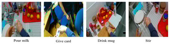
Figure 6.
Illustrative samples from the FPHA dataset.
These datasets represent significant challenges to image set classification, each emphasizing distinct aspects, such as object recognition under varying conditions (ETH-80), real-world emotional expression detection (AFEW), and complex hand gesture recognition in dynamic settings (FPHA).
6.2. Comparative Methods
To evaluate the effectiveness of the method proposed in this paper, we compare it with several existing image set classification methods:
- (1)
- Riemannian metric-based methods: affine-invariant Riemannian metric (AIRM) [16] and log-Euclidean metric (LEM) [17];
- (2)
- Subspace-based methods: mutual subspace method (MSM) [36], constrained mutual subspace method (CMSM) [37], and discriminant canonical correlations (DCC) [7];
- (3)
- Kernel-based methods: Grassmann discriminant analysis (GDA) [1], graph embedding discriminant analysis (GEDA) [38], and covariance discriminative learning (CDL) [8];
- (4)
- Riemannian manifold deep learning methods: SPD manifold network (SPDNet) [26], symmetric SPD network (SymNet) [35], discriminative multiple-manifold network (DMMNet) [39], and SPD manifold deep metric learning (SMDML) [40].
A comparison of the above methods, along with their advantages, disadvantages and characteristics, are shown in Table 1.

Table 1.
Comparison of previous image set classification methods, along with their advantages, disadvantages, and characteristics.
6.3. Experimental Settings
To ensure a fair comparison, the parameters for the aforementioned methods are adjusted based on the original literature and the source code provided by the authors. Specifically, for MSM, CMSM, and DCC, principle component analysis (PCA) is used to retain 95% of the energy for learning linear subspaces. In GDA and GEDA, cross-validation is employed to determine the number of basis vectors used for Grassmann subspaces. CDL utilizes the improved, partial least squares method for better performance. In SPDNet, the dimensions of the weight matrices are uniformly set to , , and for the AFEW and ETH-80 datasets; and , , and for the FPHA dataset. For SymNet, the activation thresholds η and ϵ are set to values consistent with those of [35] for the AFEW, FPHA, and ETH-80 datasets.
6.4. Comparisons of Methods on Three Image Sets
The results of the different image set classification algorithms used on the ETH-80, AFEW, and FPHA databases are presented in Table 2. Our proposed method, RGDA-MRMD, achieved the highest recognition rates on all three datasets. Specifically, RGDA-MRMD achieved 97.50% ± 1.68% on the ETH-80, 37.27% on the AFEW, and 88.47% on the FPHA, reflecting significant improvements over the second-best methods by 0.52%, 2.0%, and 1.3%, respectively.
Table 2.
Comparison of image set classification methods on ETH-80, AFEW, and FPHA databases.
On the ETH-80 dataset, our method significantly outperformed the baseline methods, with the second-best method (SVDML) achieving 97.00% ± 2.12%. Other methods, like AIRM, LEM, and MSM, had much lower accuracies, ranging from 85.75% to 87.00%. The superior performance of RGDA-MRMD can be attributed to its effective preservation of the geometric structure of the data and enhanced classification performance through deep feature learning.
For the AFEW dataset, which captures real-world variability in facial expressions with challenges such as varying lighting conditions, angles, occlusions, and complex backgrounds, RGDA-MRMD achieved an accuracy of 37.27%. This is 17.09% higher than the best kernel-based method, CDL, which achieved 31.83%. Baseline methods like AIRM and LEM had even lower accuracies, highlighting the robustness of our method for handling such complex datasets.
On the FPHA dataset, our method achieved 88.47%, surpassing the SymNet method, which achieved 82.75%. Baseline methods, such as AIRM, LEM, and MSM, had accuracies below 60%. The significant improvement of RGDA-MRMD on this dataset can be attributed to its ability to manage considerable variations in style, movement speed, scale, and viewpoint, making it well suited for dynamic hand gesture recognition.
The accuracy scores of 97.50 ± 1.68 for the ETH-80, 37.27 for the AFEW, and 88.47 for the FPHA reflect the challenges posed by each dataset. The lower accuracy observed for the AFEW can be attributed to its capturing of facial expressions in diverse, real-world settings characterized by varying lighting conditions, angles, occlusions, and complex backgrounds. These factors introduce considerable variability into facial expressions across different scenes, making it inherently more difficult to achieve high classification accuracy compared to controlled datasets, like the ETH-80 and FPHA. Despite these challenges, our proposed method demonstrates its superiority by achieving the highest accuracy on the AFEW dataset.
Furthermore, some interesting findings can be observed from Table 2.
Firstly, the classification accuracy of LEM for all three benchmark datasets is superior to that of AIRM, indicating that the geodesic distance between any two SPD matrices calculated by LEM better preserves the geometric structure of the data, yielding more precise results. This is primarily because this Riemannian metric is equivalent to the Euclidean metric in the SPD tangent space.
Secondly, the results for GDA are slightly inferior to those for GEDA across all the datasets, suggesting that integrating the local structure information of the data can more finely distinguish between data points, thereby enhancing classification accuracy. In contrast to GEDA and GDA, which map data onto linear subspaces, CDL utilizes the covariance information of data features for discriminative learning. By delving into the relationships between data features, CDL can extract more discriminative features, thereby improving the performance of the learning model.
Additionally, kernel-based methods (GDA, GEDA, and CDL) outperform subspace (MSM, CMSM, and DCC) and Riemannian metric-based methods (AIRM and LEM) in terms of accuracy, mainly because they introduce kernel tricks that map data to a high-dimensional feature space to capture the nonlinear structure and complex relationships within the data. This enables the kernel methods to provide a richer and more powerful representation for classifying image sets with highly nonlinear and intricate internal structures.
Lastly, the manifold deep learning methods (SPDNet and SymNet) further improve recognition accuracy because they combine deep learning with the geometric properties of Riemannian manifolds. These methods can better utilize the geometric information of the data while extracting deep features through deep networks, effectively merging geometric information and data-driven learning.
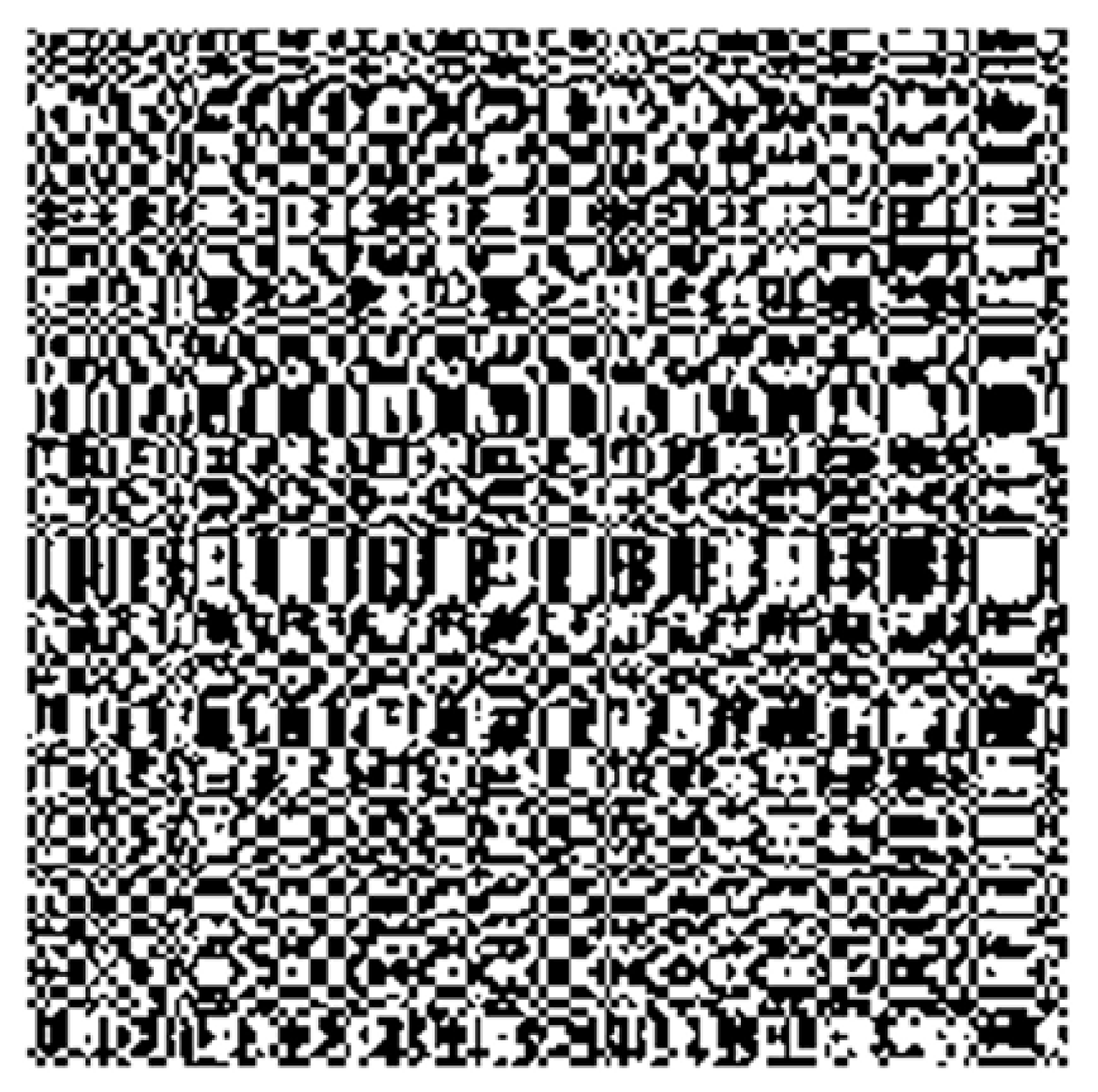
Figure 7 illustrates an example of the transformation of the ETH-80 datasets into SPD matrices, providing a clear visual representation of our method’s process.
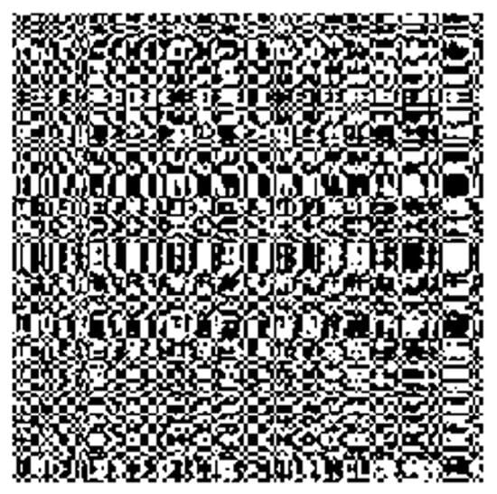
Figure 7.
Visualization of an SPD matric of a car in the ETH-80 dataset.
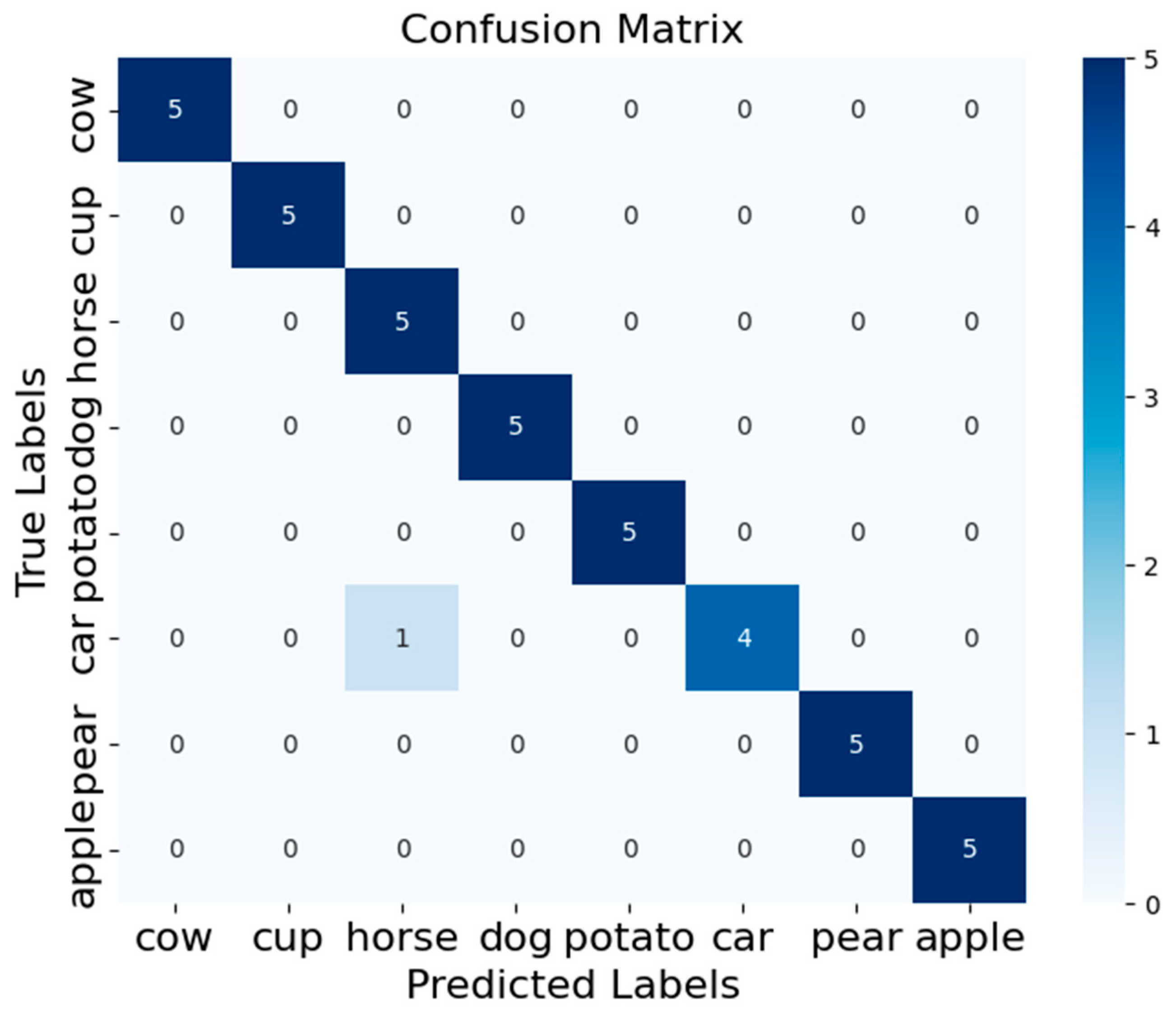
The confusion matrix, which is shown in Figure 8, demonstrates that the RDGA-MRMD method performs exceptionally well on the ETH-80 dataset, with a high overall accuracy and only a single misclassification. The high precision, recall, and F1 scores for most of the classes reflect the robustness and reliability of the proposed method. The slight misclassification in the “car” class suggests that there may be some similarity or overlap between the “car” and “horse” classes, which could be an area for further investigation or improvement of the model.
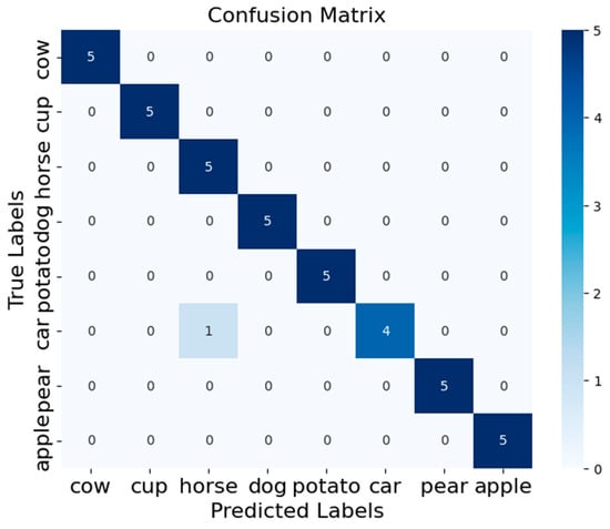
Figure 8.
The confusion matrix for our proposed method on the ETH-80 dataset.
6.5. Ablation Study on Different Discriminant Analysis Algorithms
Conducting an ablation study on different discriminant analysis algorithms, such as FDA, LFDA, and RLFDA, is essential for understanding their individual contributions to the task of image set classification. This necessity arises from the complex nature of image data, which often resides on high-dimensional manifolds with intricate structures.
The results, derived from the average of ten independent trials, as shown in Table 3, indicate a progressive improvement in classification accuracy from FDA to LFDA, and finally to RLFDA, across all three databases. Specifically, the RLFDA algorithm achieved the highest recognition rates of 97.50% on the ETH-80, 37.27% on the AFEW, and 88.47% on the FPHA. These improvements highlight the effectiveness of incorporating locality and regularization into FDA for image set classification tasks.
Table 3.
Comparative analysis of classification performance across FDA, LFDA, and RLFDA on three databases.
- ETH-80 Dataset Analysis
The ETH-80 dataset analysis shows a significant improvement in classification metrics from FDA to LFDA and then to RLFDA. The accuracy improved from 96.65% (FDA) to 97.13% (LFDA), and further to 97.50% (RLFDA), representing a cumulative increase of 0.88%. The recall and precision followed similar trends, with recall increasing from 96.65% to 97.50% (an increase of 0.88%) and precision from 96.14% to 97.90% (an increase of 1.83%). The F1 score improved from 96.39% to 97.50%, reflecting a 1.15% enhancement. These results underscore the advantage of incorporating locality and regularization, which allows RLFDA to capture intricate data structures more effectively than its predecessors.
- AFEW Dataset Analysis
On the challenging AFEW dataset, the progressive enhancements from FDA to LFDA and then to RLFDA are evident. The accuracy rose from 35.31% (FDA) to 36.78% (LFDA) and finally to 37.27% (RLFDA), resulting in a total improvement of 5.55%. The recall increased from 35.46% to 37.14%, a cumulative rise of 1.68%. The precision improved significantly from 35.88% to 38.39%, reflecting a 7.00% increase. The F1 score saw a notable enhancement from 35.67% to 37.75%, indicating a 5.83% improvement. These improvements highlight the effectiveness of RLFDA at handling real-world variability in facial expressions by leveraging the local data structure and regularization.
- FPHA Dataset Analysis
For the FPHA dataset, which involves complex hand gesture recognition, the enhancements from FDA to LFDA and then to RLFDA are substantial. The accuracy increased from 85.11% (FDA) to 86.35% (LFDA), and further to 88.47% (RLFDA), showing a total gain of 3.95%. The recall improved from 85.26% to 88.28%, a cumulative rise of 3.54%, while the precision increased from 86.01% to 89.22%, reflecting a 3.73% improvement. The F1 score saw a significant enhancement from 85.04% to 87.96%, marking a total improvement of 3.43%. These results demonstrate RLFDA’s superior ability to manage the complexities of dynamic hand gestures through the effective use of locality and regularization techniques.
These results demonstrate a clear and consistent trend of progressive enhancement in classification performance metrics across the three datasets, as more sophisticated discriminant analysis techniques are employed. The key advancements can be distilled as follows:
FDA lays the foundational strategy for discriminant analysis by optimizing class variances, but falls short in capturing the data’s local nuances, which are critical for image sets.
LFDA builds on FDA by incorporating local data insights to better manage complex distributions, thereby boosting discriminative capabilities.
RLFDA extends LFDA’s reach by integrating regularization to mitigate overfitting and enhance model robustness. It effectively leverages unlabeled data to achieve the highest accuracies, recall, precision, and F1 scores in this study.
By demonstrating these progressive enhancements, this study underscores the importance of advancing discriminant analysis techniques to capture the complex geometric structures inherent in image sets, leading to significantly improved classification performance.
6.6. Robustness Analysis
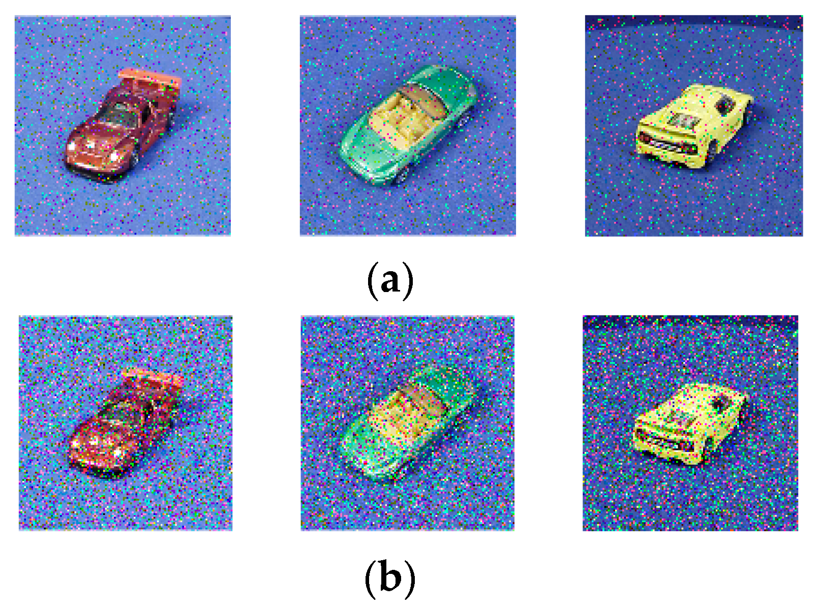
To assess the robustness of the proposed method, salt-and-pepper noise is introduced at levels of 10% and 20% into the ETH80 dataset. Figure 9 illustrates some of the instances degraded by the added noise. The rationale for employing salt-and-pepper noise lies in its capability to simulate real-world scenarios where digital images may suffer from sudden disturbances. This type of noise poses a significant challenge as it introduces extreme pixel values (0 or 255), effectively testing the algorithm’s ability to handle outliers and maintain classification accuracy.
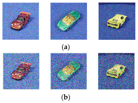
Figure 9.
Examples of image degradation due to salt-and-pepper noise. (a) 10% salt-and-pepper noise. (b) 20% salt-and-pepper noise.
Table 4 illustrates the classification performance of the various methods on the ETH-80 dataset under the influence of 10% and 20% salt-and-pepper noise. Our method consistently demonstrates remarkable robustness across all the metrics: accuracy, recall, precision, and F1 score. At a 10% noise level, RDGA-MRMD achieves an accuracy of 95.09%, which is 3.88% higher than the next best method, GEDA, with 91.54%. RDGA-MRMD also excels in recall and precision, each at 95.09%, outperforming the Riemannian deep learning method (SymNet) by 5.23% for recall and 4.97% for precision. The F1 score of 95.00% for our method is 3.84% higher than CDL, the third best, which stands at 91.49%.
Table 4.
Classification performance of different methods on ETH-80 dataset after adding salt-and-pepper noise.
When the noise level is increased to 20%, RDGA-MRMD maintains the highest performance, with an accuracy of 91.35%, showing a 3.58% increase over the next best method, GEDA, at 88.19%. Similarly, RDGA-MRMD’s recall, at 91.35%, surpasses that of SPDNet by 21.38%, and its precision of 91.93% is 9.22% higher than CDL’s 84.17%. The F1 score for RLFDA, at 91.64%, is 9.55% better than that of SymNet. These results underscore the superior robustness of RDGA-MRMD, particularly its capacity to effectively handle substantial noise by preserving the core data structure and minimizing performance degradation.
In an additional experiment conducted on the ETH-80 dataset, the robustness of the proposed method is further scrutinized by conducting a classification test. This study strategically varied the quantity of training samples to benchmark the performance of the proposed method against the other contenders, in terms of classification accuracy, as shown in Figure 10.
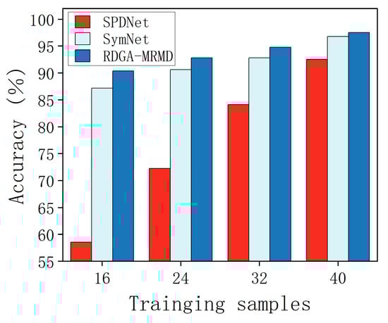
Figure 10.
Classification accuracy of different methods on ETH-80 dataset with variable training samples.
The bar chart clearly illustrates a trend: the classification accuracy for all the considered methodologies trends upward in conjunction with an increase in the volume of training samples. Notably, the RGDA-MRMD method consistently surpasses its counterparts SPDNet and SymNet at every level of training sample expansion, securing the topmost classification score across all the tested configurations. These graphical data compellingly underscore the RGDA-MRMD method’s resilience, particularly in achieving superior classification accuracy over a spectrum of training sample sizes.
6.7. Parameter Selection for Our Proposed Method
The performance of our RGDA-MRMD method relies on several key parameters, particularly in the RLFDA step. Below, we provide a detailed discussion of the rationale behind the chosen parameters and their ranges.
- Regularization Factor β
In RLFDA, the regularization term β is introduced to mitigate overfitting by incorporating information from unlabeled samples. This factor adjusts the influence of the regularization on the between-class scatter matrix and the within-class scatter matrix , respectively.
Extensive cross-validation experiments were conducted to determine the optimal values for β, which are shown in Table 5. The value was chosen from a range of [0.001, 0.01, 0.1, 1], based on the model’s performance on a validation set. The final chosen value achieved a balance between maintaining the discriminative power of the features and reducing the overfitting risks.
Table 5.
Accuracy of different regularization factors β on ETH-80, AFEW, and FPHA databases.
For our datasets (ETH-80, AFEW, and FPHA), we found that β = 0.01 yielded the best balance, enhancing the robustness of the classification without over-regularizing the scatter matrices.
- LPP Parameters γ and k
The parameter γ controls the influence of the locality-preserving projections, which ensure that points close to each other in the original space remain close in the reduced-dimensional space. The parameter k defines the number of nearest neighbors used in constructing the local neighborhood graph.
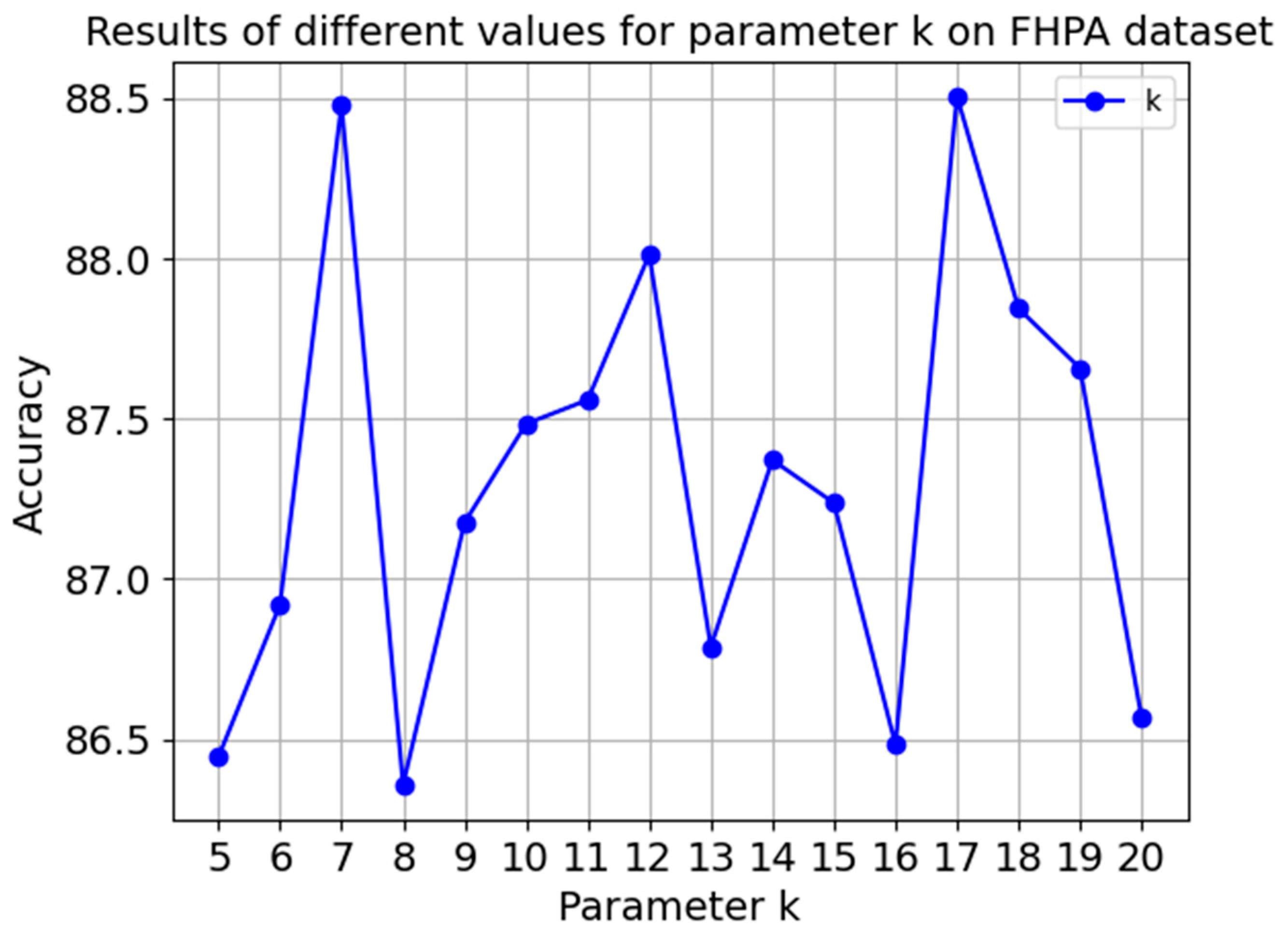
The parameter γ was determined based on the local scaling parameter approach, where it adapts to the local density of the data. We set γ according to the distance to the k-nearest neighbor, typically chosen from a range of [5, 20], which is shown in Figure 11. This choice helped to maintain local consistency while preventing too tight or too loose neighborhood definitions.
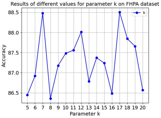
Figure 11.
Results of different values for parameter k on FHPA dataset.
It was found that setting k = 7 provided a good compromise between capturing sufficient local structure and computational efficiency. For γ, we used the median distance to the seventh nearest neighbor as the scaling factor in Equation (36).
6.8. Discussion and Insights
The results and analysis presented highlight several strengths of the RGDA-MRMD method for image set classification, particularly across diverse and challenging datasets like the ETH-80, AFEW, and FPHA. However, it is also important to consider the limitations and the broader implications of these findings.
- (1)
- Preservation of geometric structure
RGDA-MRMD effectively utilizes SPD matrices to represent image sets as covariance matrices. This representation captures the underlying variance and relationships within the data, which is crucial for distinguishing between different classes.
By projecting these SPD matrices onto the tangent space using the logarithmic map, our method reduces dimensionality while preserving the geometric structure. This step ensures that the inherent properties of the data are maintained, leading to more accurate classification.
- (2)
- Dimensionality reduction and feature extraction
Our method employs RLFDA for dimensionality reduction and feature extraction. RLFDA incorporates local data structures and regularization, enhancing model robustness and preventing overfitting, especially in scenarios with limited labeled data.
The emphasis on local characteristics ensures that the discriminant analysis accounts for the proximity of the data points within their respective classes. This approach refines classification boundaries, leading to improved performance compared to traditional FDA.
- (3)
- Geodesic filtering and remapping
After dimensionality reduction, the projection plane of RLFDA is reconstructed using a geodesic filtering algorithm, which establishes a separable tangent plane. This technique effectively segregates points based on maximum inter-class distance and minimum intra-class distance.
The exponential map is then used to remap the separable covariance feature data back into the Riemannian manifold space. This step preserves the unique topological structure of SPD matrices, such as their positive definiteness, which is critical for accurate classification.
- (4)
- MRMD algorithm
The final classification is performed using the MRMD algorithm, which accurately classifies the data points on the Riemannian manifold. This approach leverages the geometric properties of the data, resulting in higher classification accuracy and effectiveness.
- (5)
- Dependency on unlabeled data quality and quantity
One significant limitation of the RGDA-MRMD method is its reliance on the availability and quality of unlabeled data for augmentation. Insufficient or poor-quality unlabeled data may hinder the method’s performance, impacting its accuracy and generalization capability across varied datasets.
- Scenarios Most Favorable to RGDA-MRMD
- (1)
- High-dimensional data with complex structures
RGDA-MRMD is particularly effective for datasets with high-dimensional data and complex structures, where preserving the geometric properties is crucial. The method’s ability to handle SPD matrices and perform dimensionality reduction while maintaining these properties leads to its superior performance.
- (2)
- Scenarios with limited labeled data
The regularization component of RLFDA enhances the robustness of the model by preventing overfitting. This feature is especially beneficial in scenarios where labeled data are limited, allowing the method to generalize better than other approaches.
- (3)
- Datasets with high intra-class variability
The method’s emphasis on local data structures ensures that it can effectively handle datasets with high intra-class variability. By refining classification boundaries based on local characteristics, RGDA-MRMD improves accuracy when distinguishing between classes with subtle differences.
- (4)
- Real-world applications with noise and variability
RGDA-MRMD demonstrates robustness in handling noisy environments and real-world variability. The geodesic filtering and remapping steps, combined with the MRMD algorithm, ensure that the method can accurately classify data despite the presence of noise and other variations.
7. Conclusions
In conclusion, this paper successfully develops and validates a novel method called RGDA-MRMD for image set classification leveraging SPD manifolds. It shows significant improvements in classification accuracy across the ETH-80, AFEW, and FPHA datasets, with scores of 97.50%, 37.27%, and 88.47%, respectively. Through an ablation study and robustness analysis, the superiority of our method over the state-of-the-art comparison methods is demonstrated, along with its superior resilience to noise interference, underscoring its practical applicability in real-world scenarios. The use of SPD matrices for image representation, coupled with the innovative projection onto tangent spaces and the application of RLFDA, is proven to be particularly effective. These findings suggest that incorporating the Riemannian geometric structure of data into discriminant algorithms can significantly enhance classification performance.
Looking ahead, our aim is to expand the application of our method to other datasets, especially for tackling complex classification tasks within the realm of electrical engineering. Moreover, a reduction in the computational complexity of the Riemannian geometry methods is paramount, as it is significant for the improvement of the computational efficiency and scalability of the proposed method.
Author Contributions
Conceptualization, Z.L. and F.F.M.E.-S.; methodology, Z.L.; software, Z.L. and H.Q.; validation, F.F.M.E.-S., N.A.L. and H.Q.; formal analysis, Z.L.; investigation, Z.L.; resources, T.J.; data curation, F.F.M.E.-S.; writing—original draft preparation, Z.L.; writing—review and editing, F.F.M.E.-S., N.A.L., H.Q. and T.J.; visualization, Z.L.; supervision, F.F.M.E.-S. and T.J.; project administration, F.F.M.E.-S. and T.J.; funding acquisition, F.F.M.E.-S. and T.J. All authors have read and agreed to the published version of the manuscript.
Funding
This project was supported via funding from Prince Sattam bin Abdulaziz University (Project Number PSAU/2024/R/1445) and the National Natural Science Foundation of China (52077081).
Data Availability Statement
The data that support the findings of this study are available from the corresponding author upon reasonable request.
Conflicts of Interest
The authors declare no conflicts of interest.
References
- Hamm, J.; Lee, D.D. Grassmann discriminant analysis: A unifying view on subspace-based learning. In Proceedings of the 25th International Conference on Machine Learning, Helsinki, Finland, 5–9 July 2008; pp. 376–383. [Google Scholar]
- Bansal, M.; Kumar, M.; Sachdeva, M.; Mittal, A. Transfer learning for image classification using VGG19: Caltech-101 image data set. J. Ambient Intell. Humaniz. Comput. 2023, 14, 609–620. [Google Scholar] [CrossRef] [PubMed]
- Xie, X.; Zou, X.; Yu, T.; Tang, R.; Hou, Y.; Qi, F. Multiple graph fusion based on Riemannian geometry for motor imagery classification. Appl. Intell. 2022, 52, 9067–9079. [Google Scholar] [CrossRef]
- Gao, Y.; Sun, X.; Meng, M.; Zhang, Y. Eeg emotion recognition based on enhanced spd matrix and manifold dimensionality reduction. Comput. Biol. Med. 2022, 146, 606. [Google Scholar] [CrossRef] [PubMed]
- Li, X.; Yang, Y.; Hu, N.; Cheng, Z.; Shao, H.; Cheng, J. Maximum margin riemannian manifold-based hyperdisk for fault diagnosis of roller bearing with multi-channel fusion covariance matrix. Adv. Eng. Inf. 2022, 51, 513. [Google Scholar] [CrossRef]
- Zhou, X.; Ling, B.W.; Ahmed, W.; Zhou, Y.; Lin, Y.; Zhang, H. Multivariate phase space reconstruction and Riemannian manifold for sleep stage classification. Biomed. Signal Process. Control 2024, 88, 105572. [Google Scholar] [CrossRef]
- Kim, T.; Kittler, J.; Cipolla, R. Discriminative learning and recognition of image set classes using canonical correlations. IEEE Trans. Pattern Anal. Mach. Intell. 2007, 29, 1005–1018. [Google Scholar] [CrossRef] [PubMed]
- Wang, R.; Guo, H.; Davis, L.S.; Dai, Q. Covariance discriminative learning: A natural and efficient approach to image set classification. In Proceedings of the 2012 IEEE Conference on Computer Vision and Pattern Recognition, Providence, RI, USA, 16–21 June 2012; pp. 2496–2503. [Google Scholar]
- Krizhevsky, A.; Sutskever, I.; Hinton, G.E. Imagenet classification with deep convolutional neural networks. Adv. Neural Inf. Process. Syst. 2012, 25, 84–90. [Google Scholar] [CrossRef]
- He, K.; Zhang, X.; Ren, S.; Sun, J. Deep residual learning for image recognition. In Proceedings of the IEEE Conference on Computer Vision and Pattern Recognition, Las Vegas, NV, USA, 27–30 June 2016; pp. 770–778. [Google Scholar]
- Roweis, S.T.; Saul, L.K. Nonlinear dimensionality reduction by locally linear embedding. Science 2000, 290, 2323–2326. [Google Scholar] [CrossRef] [PubMed]
- Tenenbaum, J.B.; Silva, V.D.; Langford, J.C. A global geometric framework for nonlinear dimensionality reduction. Science 2000, 290, 2319–2323. [Google Scholar] [CrossRef] [PubMed]
- Harandi, M.; Sanderson, C.; Shen, C.; Lovell, B.C. Dictionary learning and sparse coding on Grassmann manifolds: An extrinsic solution. In Proceedings of the IEEE International Conference on Computer Vision, Sydney, Australia, 1–8 December 2013; pp. 3120–3127. [Google Scholar]
- Harandi, M.; Hartley, R.; Shen, C.; Lovell, B.; Sanderson, C. Extrinsic methods for coding and dictionary learning on Grassmann manifolds. Int. J. Comput. Vis. 2015, 114, 113–136. [Google Scholar] [CrossRef]
- Huang, W.; Sun, F.; Cao, L.; Zhao, D.; Liu, H.; Harandi, M. Sparse coding and dictionary learning with linear dynamical systems. In Proceedings of the IEEE Conference on Computer Vision and Pattern Recognition, Las Vegas, NV, USA, 27–30 June 2016; pp. 3938–3947. [Google Scholar]
- Pennec, X.; Fillard, P.; Ayache, N. A Riemannian framework for tensor computing. Int. J. Comput. Vis. 2006, 66, 41–66. [Google Scholar] [CrossRef]
- Arsigny, V.; Fillard, P.; Pennec, X.; Ayache, N. Geometric means in a novel vector space structure on symmetric positive-definite matrices. SIAM J. Matrix Anal. Appl. 2007, 29, 328–347. [Google Scholar] [CrossRef]
- Huang, Z.; Wang, R.; Shan, S.; Chen, X. Projection metric learning on Grassmann manifold with application to video based face recognition. In Proceedings of the IEEE Conference on Computer Vision and Pattern Recognition, Boston, MA, USA, 7–12 June 2015; pp. 140–149. [Google Scholar]
- Nguyen, X.S. Geomnet: A neural network based on riemannian geometries of spd matrix space and cholesky space for 3d skeleton-based interaction recognition. In Proceedings of the IEEE/CVF International Conference on Computer Vision, Montreal, BC, Canada, 11–17 October 2021; pp. 13379–13389. [Google Scholar]
- Zhang, T.; Zheng, W.; Cui, Z.; Zong, Y.; Li, C.; Zhou, X.; Yang, J. Deep manifold-to-manifold transforming network for skeleton-based action recognition. IEEE Trans. Multimed. 2020, 22, 2926–2937. [Google Scholar] [CrossRef]
- Quang, M.H.; Biagio, M.S.; Murino, V. Log-Hilbert-Schmidt metric between positive definite operators on Hilbert spaces. Adv. Neural Inf. Process. Syst. 2014, 27, 388–396. [Google Scholar]
- Jayasumana, S.; Hartley, R.; Salzmann, M.; Li, H.; Harandi, M. Kernel methods on Riemannian manifolds with Gaussian RBF kernels. IEEE Trans. Pattern Anal. Mach. Intell. 2015, 37, 2464–2477. [Google Scholar] [CrossRef]
- Huang, Z.; Wang, R.; Shan, S.; Li, X.; Chen, X. Log-euclidean metric learning on symmetric positive definite manifold with application to image set classification. In Proceedings of the International Conference on Machine Learning, Lille, France, 7–9 July 2015; pp. 720–729. [Google Scholar]
- Tuzel, O.; Porikli, F.; Meer, P. Pedestrian detection via classification on riemannian manifolds. IEEE Trans. Pattern Anal. Mach. Intell. 2008, 30, 1713–1727. [Google Scholar] [CrossRef] [PubMed]
- Çetingül, H.E.; Wright, M.J.; Thompson, P.M.; Vidal, R. Segmentation of high angular resolution diffusion MRI using sparse Riemannian manifold clustering. IEEE Trans. Med. Imaging 2013, 33, 301–317. [Google Scholar] [CrossRef] [PubMed]
- Huang, Z.; Van Gool, L. A riemannian network for spd matrix learning. In Proceedings of the AAAI Conference on Artificial Intelligence, San Francisco, CA, USA, 4–9 February 2017; pp. 2036–2042. [Google Scholar]
- Kalunga, E.K.; Chevallier, S.; Barthélemy, Q.; Djouani, K.; Monacelli, E.; Hamam, Y. Online SSVEP-based BCI using Riemannian geometry. Neurocomputing 2016, 191, 55–68. [Google Scholar] [CrossRef]
- Stefani, G.; Boscain, U.; Gauthier, J.; Sarychev, A.; Sigalotti, M. Geometric Control Theory and Sub-Riemannian Geometry; Springer: Berlin/Heidelberg, Germany, 2014. [Google Scholar]
- Fisher, R.A. The use of multiple measurements in taxonomic problems. Ann. Eugen. 1936, 7, 179–188. [Google Scholar] [CrossRef]
- Sugiyama, M. Dimensionality reduction of multimodal labeled data by local fisher discriminant analysis. J. Mach. Learn. Res. 2007, 8, 1027–1061. [Google Scholar]
- Lu, N.; Lin, H.; Lu, J.; Zhang, G. A customer churn prediction model in telecom industry using boosting. IEEE Trans. Ind. Inform. 2012, 10, 1659–1665. [Google Scholar] [CrossRef]
- Leibe, B.; Schiele, B. Analyzing appearance and contour based methods for object categorization. In Proceedings of the IEEE Computer Society Conference on Computer Vision and Pattern Recognition, Madison, WI, USA, 18–20 June 2003; p. 409. [Google Scholar]
- Dhall, A.; Goecke, R.; Joshi, J.; Sikka, K.; Gedeon, T. Emotion recognition in the wild challenge 2014: Baseline, data and protocol. In Proceedings of the 16th International Conference on Multimodal Interaction, Istanbul, Turkey, 12–16 November 2014; pp. 461–466. [Google Scholar]
- Garcia-Hernando, G.; Yuan, S.; Baek, S.; Kim, T. First-person hand action benchmark with rgb-d videos and 3d hand pose annotations. In Proceedings of the IEEE Conference on Computer Vision and Pattern Recognition, Salt Lake City, UT, USA, 18–23 June 2018; pp. 409–419. [Google Scholar]
- Wang, R.; Wu, X.; Kittler, J. SymNet: A simple symmetric positive definite manifold deep learning method for image set classification. IEEE Trans. Neural Netw. Learn. Syst. 2021, 33, 2208–2222. [Google Scholar] [CrossRef] [PubMed]
- Yamaguchi, O.; Fukui, K.; Maeda, K. Face recognition using temporal image sequence. In Proceedings of the Third IEEE International Conference on Automatic Face and Gesture Recognition, Nara, Japan, 14–16 April 1998; pp. 318–323. [Google Scholar]
- Fukui, K.; Maki, A. Difference subspace and its generalization for subspace-based methods. IEEE Trans. Pattern Anal. Mach. 2015, 37, 2164–2177. [Google Scholar] [CrossRef] [PubMed]
- Harandi, M.T.; Sanderson, C.; Shirazi, S.; Lovell, B.C. Graph embedding discriminant analysis on Grassmannian manifolds for improved image set matching. In Proceedings of the IEEE Conference on Computer Vision and Pattern Recognition, Colorado Springs, CO, USA, 20–25 June 2011; pp. 2705–2712. [Google Scholar]
- Wu, H.; Wang, W.; Xia, Z. A discriminative multiple-manifold network for image set classification. Appl. Intell. 2023, 53, 25119–25134. [Google Scholar] [CrossRef]
- Wang, R.; Wu, X.J.; Chen, Z.; Hu, C.; Kittler, J. SPD manifold deep metric learning for image set classification. IEEE Trans. Neural Netw. Learn. Syst. 2024. early access. [Google Scholar]


Disclaimer/Publisher’s Note: The statements, opinions and data contained in all publications are solely those of the individual author(s) and contributor(s) and not of MDPI and/or the editor(s). MDPI and/or the editor(s) disclaim responsibility for any injury to people or property resulting from any ideas, methods, instructions or products referred to in the content. |
© 2024 by the authors. Licensee MDPI, Basel, Switzerland. This article is an open access article distributed under the terms and conditions of the Creative Commons Attribution (CC BY) license (https://creativecommons.org/licenses/by/4.0/).