Abstract
Accurately predicting the trajectory of carbon emissions is vital for achieving a sustainable shift toward a green and low-carbon future. Hence, this paper created a novel model to examine the driver analysis and integrated prediction for Chinese carbon emission, a large carbon-emitting country. The logarithmic mean divisia index (LMDI) approach initially served to decompose the drivers of carbon emissions, analyzing the annual and staged contributions of these factors. Given the non-stationarity and non-linear characteristics in the data sequence of carbon emissions, a decomposition–integration prediction model was proposed. The model employed the empirical mode decomposition (EMD) model to decompose each set of data into a series of components. The various carbon emission components were anticipated using the long short-term memory (LSTM) model based on the deconstructed impacting factors. The aggregate of these predicted components constituted the overall forecast for carbon emissions. The result indicates that the EMD-LSTM model greatly decreased prediction errors over the other comparable models. This paper makes up for the gap in existing research by providing further analysis based on the LMDI method. Additionally, it innovatively incorporates the EMD method into the carbon emission study, and the proposed EMD-LSTM prediction model effectively addresses the volatility characteristics of carbon emissions and demonstrates excellent predictive performance in carbon emission prediction.
MSC:
91B76
1. Introduction
Climate change, with global warming as a prominent feature, has profound impacts on human survival and development. It is regarded as one of the gravest global crises and challenges faced by contemporary human society [1,2]. And, greenhouse gases (GHG) emitted from human activities are the primary drivers of global warming [3]. Owing to the tremendous socio-economic advancement in recent years, there has been an enormous rise in human utilization of fossil fuels, resulting in the quick accumulation of carbon emissions and exacerbating global warming [4]. Currently, the world is initiating the path of carbon neutrality, with widespread international consensus on green and low-carbon growth [5,6]. By concluding the Paris Agreement, a new paradigm has been initiated for global climate governance, where all parties commit to participation and undertake actions collectively [7].
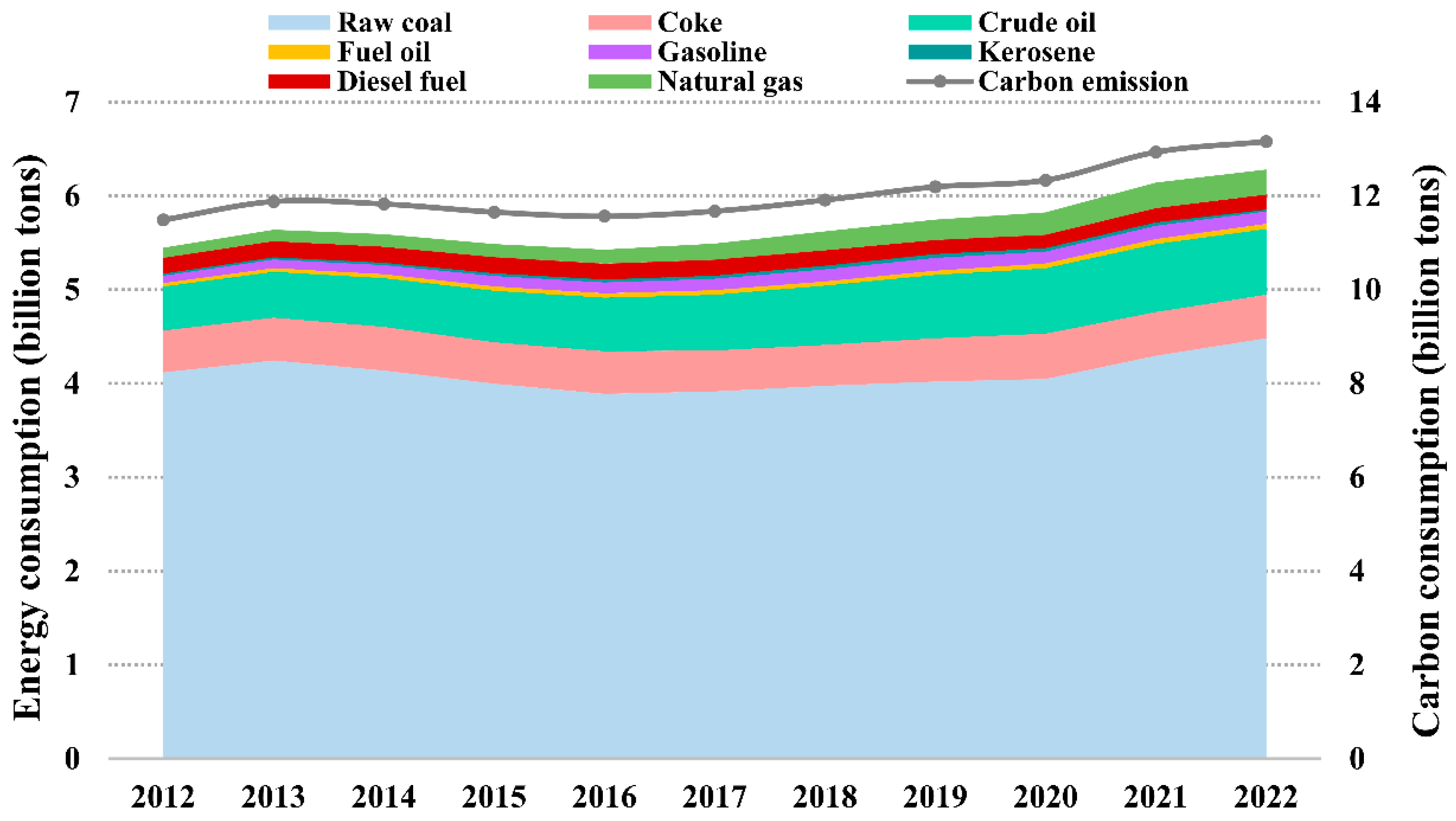
As the primary energy consumer and GHG emitter globally, China holds major leverage to guide the path of reducing carbon emissions worldwide [8,9]. The resource endowment of “rich in coal but poor in oil and gas” has prolonged the Chinese energy consumption structure to be dominated by coal. And, the excessive consumption of fossil fuels is a vital factor in increasing carbon emissions (see Figure 1). China is also the largest developing nation; therefore, it is keen to fulfill its GHG reduction obligations, and it is committed to hitting peak emissions before 2030 and for carbon neutrality by 2060 [10,11]. With the overarching goal of “dual carbon”, the Chinese government has initiated a range of specific carbon reduction targets [12,13]. For instance, “the CO2 emissions are slated to decrease by 18% for 2021–2025… achieving a reduction of over 65% in CO2 emissions per unit of GDP by 2030 compared to the levels in 2005”. All policy objectives clearly outline the carbon reduction postures for China at various future phases, and there is no doubt that the carbon emissions will certainly be controlled and mitigated. However, due to the urgency of the timeline and the complexity of the environment, it remains uncertain whether China can achieve its planned targets as scheduled [14]. Therefore, accurately predicting carbon emissions may aid the Chinese government in implementing carbon policies that make sense and attaining dual carbon targets methodically and scientifically [15].

Figure 1.
The energy consumption and carbon emissions in China for 2012–2022.
Exploring the factors impacting carbon emissions is essential for precisely estimating their changes. Numerous academics have examined the variables that affect carbon emissions, and the majority of the techniques used are based on the STIRPAT model and decomposition analysis [16]. The STIRPAT model is a scalable randomized environmental effects evaluation model developed by Dietz et al. [17]. With the use of the STIRPAT model, Chai et al. [18] investigated the variables affecting carbon emissions in Xinjiang Province. Zhang et al. [19] confirmed that economic growth is the primary factor impacting carbon emissions in China. Guo et al. [20] examined the factors influencing carbon emissions in the Yangtze River Delta region by using the improved STIRPAT model and discovered that the main contributors to carbon emissions varied significantly among provinces. Li et al. [21] identified GDP per capita, urbanization rate, and resident population as the main drivers of carbon emissions from residential buildings through this model. Decomposition analysis methods primarily consist of two types: structural decomposition analysis (SDA) and index decomposition analysis (IDA) [22]. The former mainly relies on input–output tables, while the latter is simpler to operate and only requires the use of sectoral aggregated data for calculation, so it is more widely used. In particular, the LMDI method in IDA makes extensive use in the analysis of energy consumption and carbon emission drivers [23,24]. By employing an extended Kaya and LMDI, Hao et al. [25] examined the factors influencing China’s carbon emissions for 1980–2020. Their results show that prices and energy intensity act as inhibitors to the country’s growth in carbon emissions, revealing that prices and energy intensity act as inhibitors on the Chinese growth in carbon emissions, while energy intensity and prices act as inhibiting factors. Zhang and Li [26] investigated the variables affecting carbon emissions in the construction sector, with results indicating the main contributors to carbon emissions. Peng and Liu [27] derived from the Kaya-LMDI model that the economic output and the energy intensity effect are the two key factors influencing carbon emissions from coal consumption in China.
Regarding carbon emissions prediction, there exist various methods in academia. Wang and Ye [28] developed a nonlinear grey variate algorithm for forecasting carbon emissions from the use of fossil fuels in China for 2014–2020. The MNGM-ARIMA and MNGM-BPNN models were developed by Wang et al. [29] to project carbon emissions in China, the U.S., and India. Ma et al. [30] applied scenario analysis and Monte Carlo simulation to anticipate the peak carbon emissions of China’s tourism industry. Ye et al. [31] created an improved dynamic time-lagged finite grey model to address the dynamic lag relationship in carbon emissions prediction. Luo et al. [32] developed a system dynamics approach to forecasting the futuristic carbon dioxide emission trends for the Greater Bay Area and surrounding cities. Rao et al. [33] modeled a ridge regression-based STIRPAT extended model to measure the carbon emissions in Hubei Province.
While the above model requires relatively few parameters and can be easily trained, the fitting effect is ineffective in dealing with nonlinear problems, prompting many researchers to employ machine learning methods for prediction. Fang et al. [34] introduced an improved PSO algorithm for optimizing Gaussian process regression in carbon emission prediction, which is superior to traditional forecasting ways. Zhu et al. [35] introduced an integrated LSSVM model with a hybrid kernel function to reach the carbon intensity target of China. Niu et al. [36] constructed a generalized regression neural network prediction model optimized by an improved fireworks algorithm to verify if China can meet its carbon emissions commitments by 2030. Although the machine learning models can effectively solve the nonlinear fitting problem, they are prone to local optimization and overfitting problems. LSTM, with its ability to maintain long-term dependencies and handle gradient issues, is a powerful tool for time series prediction tasks, including the prediction of energy fields like solar energy consumption in the US. [37], natural gas consumption [38], and carbon emissions in China [39,40].
The existing study has explored various aspects of carbon emission forecasting, but partial insufficiencies remain. Firstly, the LMDI method holds wide application in the energy and environment field due to its residue-free decomposition results and ease of operation. However, there is an extremely limited number of studies that make further in-depth predictions on the LMDI decomposition findings, so this paper attempts to increase the range of viewpoints on the study of carbon emissions. Secondly, carbon emission forecasting research has mostly focused on methodological innovations, with few models having pre-processing operations performed on them. Whether using time series models or machine learning models for carbon emission forecasting, avoiding the influence of nonlinearity and volatility is challenging. It may make it difficult to completely solve the issue by simply relying on improving forecasting methods. Therefore, this paper utilizes the EMD approach to predict carbon emissions, decomposes carbon emissions and the influencing factors into multiple components, and constructs a carbon emission prediction model based on the various types of components obtained by EMD. Thirdly, as a recurrent neural network architecture, LSTM can capture and memorize long, sequence-dependent features, which is particularly suitable for dealing with nonlinear problems in time series data. By incorporating the LSTM model into carbon emission prediction, it can compensate for the limitations of traditional physical models in accurately describing complex spatial–temporal variations.
The innovations and contributions of this paper are as follows.
- (1)
- A hybrid LMDI-EMD-LSTM prediction model is innovatively proposed. Factor decomposition is carried out using the LMDI method, and based on the decomposed findings, the EMD-LSTM integrated model is constructed to anticipate carbon emissions.
- (2)
- The decomposition results of the LMDI method have no residuals and can successfully prevent the occurrence of the pseudo-regression problem. Therefore, this paper applies the LMDI method to examine the elements that influenced China’s carbon emissions from 1980 to 2022, and it analyses in detail the contribution of each decomposition effect to carbon emissions by year and stage.
- (3)
- The accuracy of carbon emission forecasts is affected by the fact that carbon emissions and their factor series are usually nonlinear and volatile. Hence, this paper adopts the EMD model to preprocess the carbon emission series and decompose each non-stationary series into multiple components separately to alleviate the volatility of the series.
- (4)
- Based on each carbon emission influencing factor component after EMD decomposition, the LSTM prediction model for carbon emissions is constructed. The EMD-LSTM model outperforms the benchmark model in terms of prediction accuracy, with significantly lower error indications across all metrics.
2. Methods and Data
2.1. Methodology
2.1.1. Logarithmic Mean Divisia Index
The LMDI is a technique used for factor decomposition analysis that is derived from an extended version of the Kaya identity [41]. Due to its benefits like the convenient decomposition process and residual-free results, it is currently widely applied to factor studies in various fields. Hence, this research employs the LMDI approach to examine the factors that influence carbon emissions. The decomposition formula is as follows:
where represent the carbon emissions and energy consumption of energy source type i in year t, and denote the total carbon emissions, total energy consumption, GDP, and population in year t, respectively.
Meanwhile, concerning the LMDI method proposed by Ang [42], this paper categorizes the influencing factors of carbon emissions into the carbon emission coefficient effect (), energy structure effect (), energy intensity effect (), economic development effect (), and population size effect (). Specifically, while calculating the comprehensive impact effects of carbon emissions, the carbon emission coefficient effect is taken to be 0, because the carbon emission coefficients of different energy source types stay constant. Consequently, the LMDI decomposition expression for China’s carbon emissions is as follows:
To further assess the impact of each influencing factor on carbon emissions, and referring to Hao et al. [25], this paper proceeds to calculate the relative contribution rates of each influencing factor:
where indicates the relative contribution of the ith impact effect.
2.1.2. Empirical Mode Decomposition
The EMD is a novel time–frequency analysis method that can effectively handle non-linear or non-stationary signals [43]. Through the hierarchical decomposition of EMD, a series of intrinsic modal functions (IMFs) and a trend component are eventually obtained. The specific decomposition steps of EMD are as follows:
(1) For an original data sequence , by performing cubic spline interpolation, all its local maxima are determined as the upper envelope, and all local minima are determined as the lower envelope. Using it to represent the mean of the upper and lower envelopes, the component is obtained as follows:
(2) Determine whether satisfies the conditions for an IMF, which involves the following two main aspects: (1) number of extrema: the number of extrema (local maxima and local minima) of the IMF should be equal to or differ by at most one; (2) zero crossing mean: across the entire data sequence, the mean of the upper and lower envelopes must cross zero one time. If it does not satisfy these conditions, then consider it as the new and repeat the above process.
The process is repeated until satisfies the IMF condition, which results in the first IMF and the residual component of the signal .
(3) Continue the decomposition by following step (2) until the obtained residual component satisfies the given termination conditions. The decomposition process ends with several IMFs and residual components.
The original sequence can be expressed as the sum of IMFs and residual components:
2.1.3. Long Short-Term Memory Networks
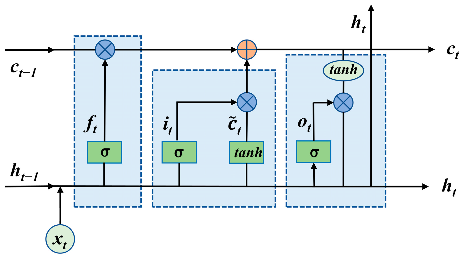
LSTM is an extension of the recurrent neural network (RNN). It has a good memory function and can effectively solve the gradient explosion issue. It is mainly composed of the basic structure of the forget gate, the input gate, and the output gate, where the gate realizes the function of forgetting or remembering. The basic structure of the LSTM model is shown in Figure 2.
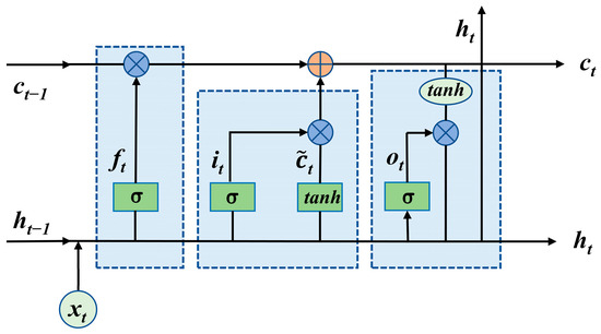
Figure 2.
The basic structure of the LSTM model.
In the forget gate, the input from the current moment and the output from the previous moment are used as inputs to a sigmoid function, designed to control the extent to which the state of the previous cell has been forgotten. The input gate is combined with the tanh function to control the amount of new input information. The output layer determines the output information, which mainly utilizes the tanh function to process the current cell state, followed by combining the weights obtained from the sigmoid function to filter some cell information and obtain the output for the next moment. The calculation formulas involved are as follows:
where are defined as the forget gate, input gate, and output gate. and represent the current input memory and cell state. and indicate the input and output at time t, W and b denote the corresponding weight coefficients and bias terms, σ is the sigmoid function, and tanh is the hyperbolic tangent function.
2.1.4. Carbon Emissions Forecasting Based on the LMDI-EMD-LSTM Model
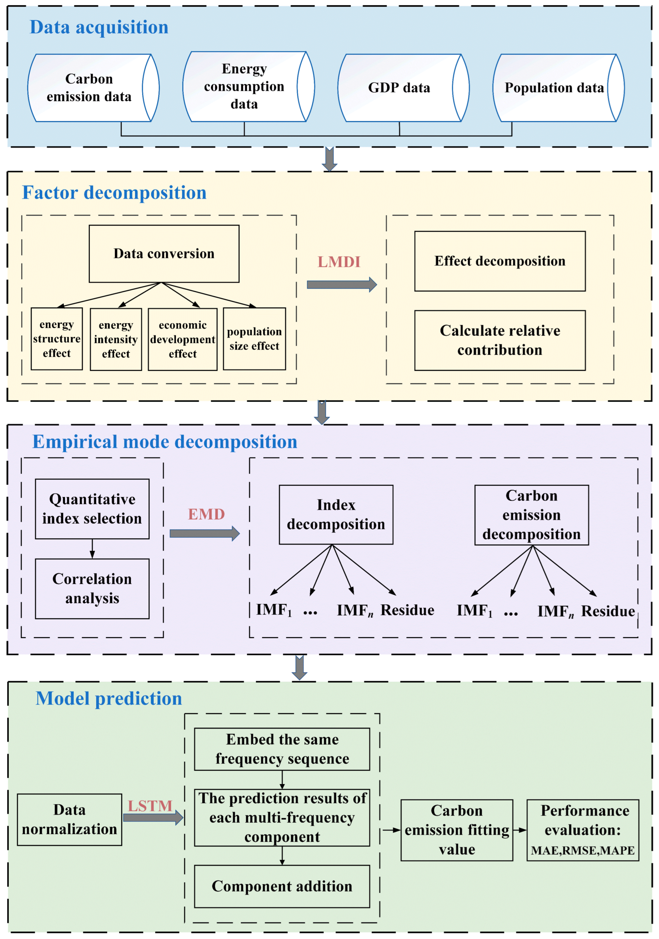
The carbon emission prediction process using the LMDI-EMD-LSTM model is illustrated in Figure 3, which mainly involves three major steps. Firstly, to effectively identify the impact of various factors on carbon emissions in China, this paper employs the LMDI method for factor analysis and specifically measures the degree of influence of each factor. Secondly, the EMD method is introduced to alleviate the nonlinearity and volatility of carbon emissions and their influencing factors, and the IMFs and residual values of each subsequence can be obtained. Finally, the components of the carbon emission influencing factors derived from the EMD processing served as the input variables, and the LSTM model is employed to predict each component of the carbon emissions. The fitted value of the carbon emissions is the sum of the IMFs and the trend component of the predicted decomposition.
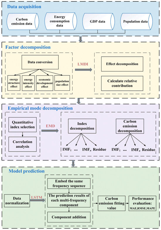
Figure 3.
Carbon emission prediction flow obtained via LMDI-EMD-LSTM modeling.
2.2. Data Sources
Taking China’s carbon emissions as the research object, this study selected relevant data for 1980–2022 to forecast. When the factorization of China’s carbon emissions using the LMDI leads to five effects, the specific variable values involved are carbon emissions, each type of sub-energy consumption, GDP, and population size. The data on energy consumption and population size are directly sourced from the China Energy Statistics Yearbook and the China Statistics Yearbook. Meanwhile, to effectively eliminate the influence of price changes, the GDP from 1980 serves as the basis for constant price processing, where the GDP and its index values were obtained from the National Bureau of Statistics of China. As direct data on carbon emissions are unavailable, this study employs the emission factor method to estimate China’s carbon emissions. And, considering that fossil energy consumption is the main source of carbon emissions [44], this study adopts energy consumption as the research perspective for analyzing China’s carbon emissions. Since electricity does not directly generate CO2, and to prevent redundancies in calculations, carbon emissions resulting from electricity consumption are excluded from consideration [45]. Ultimately, the analysis encompasses carbon emissions from eight fossil fuels: raw coal, coke, crude oil, fuel oil, gasoline, kerosene, diesel fuel, and natural gas. The carbon emission factors for various energy sources are shown in Table 1. And, the specific measurement formula for carbon emissions is as follows:

Table 1.
Carbon emission factors for various energy sources.
C represents the total carbon emissions. ADi and EFi denote the consumption and carbon emission factor of the ith type of energy source, while NCVi, CCi, and Oi are the average low calorific value, carbon content per unit calorific value, and oxidation efficiency of the i-th type of energy source, respectively. The factor 44/12 accounts for the molecular weight ratio of CO2 to C.
3. Results and Discussion
3.1. Factor Decomposing with the LMDI Model
By applying the LMDI method, the annual contribution value of each effect to carbon emissions from 1980 to 2022 can be derived, and the results of the specific contribution value of each influencing effect are shown in Table 2. Additionally, Figure 4 illustrates the patterns of each effect.
Table 2.
Factor decomposition of carbon emissions in China from 1980 to 2022 (unit: million tons).
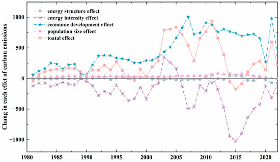
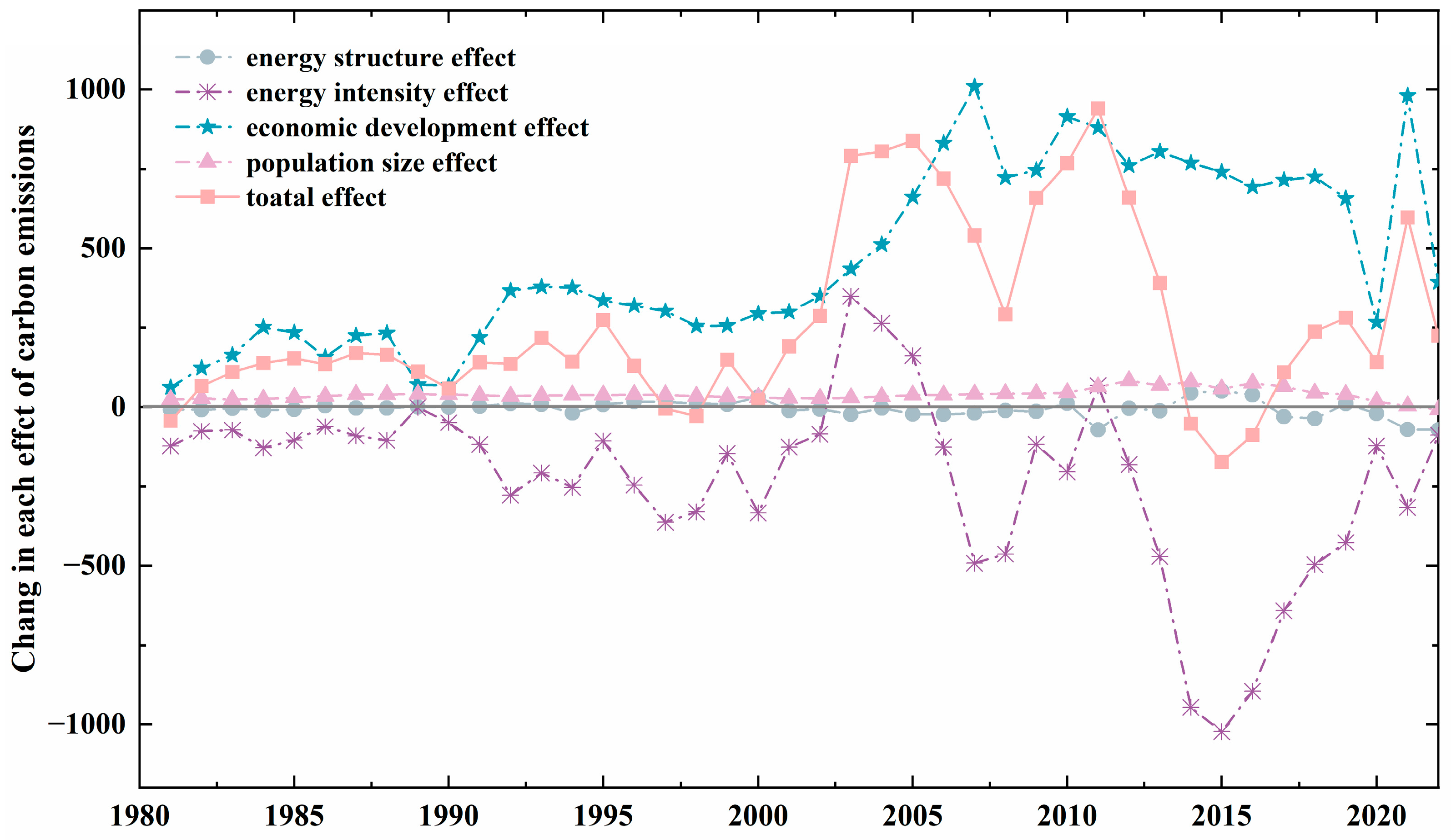
Figure 4.
Changes in the factor decomposition of carbon emissions.
The LMDI decomposition analysis clearly indicates that China’s total carbon emissions have been consistently rising. Over the period from 1980 to 2022, the total carbon emissions increased by 11,401.35 million tons. Notably, the energy structure effect and energy intensity effect present a negative inhibitory impact on the growth of carbon emissions, with specific contribution rates of −1.93% and −84.09%. Conversely, the economic development effect and population size effect exert a positive stimulating influence, with specific contribution rates of 171.59% and 14.42%. Furthermore, this suggests that both the energy intensity and economic development effect are the primary influencing factors affecting carbon emissions. However, the absolute contribution value of the economic development effect typically surpasses that of the energy intensity structure effect. As a result, the carbon emissions in China overall maintain a continuous upward trend, which is in accordance with the conclusions reached by Ji et al. [46].
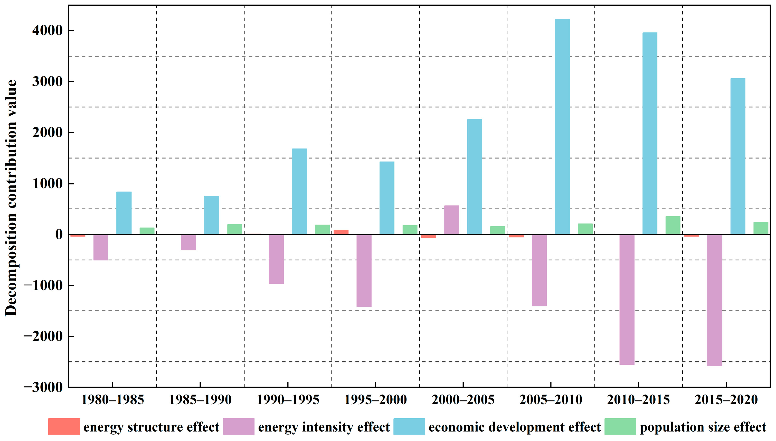
To further conduct a more in-depth examination of the influence of different factors on carbon emissions, this paper categorizes the time from 1980 to 2020 into five-year intervals, which follows the planning horizon of Chinese policies. The specific contribution value variations in each effect during these stages are depicted in Figure 5. Both the energy intensity effect and economic development effect are undoubtedly the crucial influencing factors in the growth of carbon emissions across all stages. Specifically, the energy intensity effect exhibits a substantial negative contribution of −2583.94 million tons during 2015–2020, whereas the economic development effect demonstrates a significant positive contribution of 4226.33 million tons during the period of 2005–2010. The population size effect consistently maintained a stable positive contribution throughout all stages. Although the energy structure effect showed positive contributions during the periods of 1985–2000 and 2011–2015, its overall contribution for the entire period of 1980–2022 remained negative.

Figure 5.
Factor decomposition of carbon emissions in phases.
There is an inconsistency in the contribution of the energy structure effects to carbon emissions, manifesting as positive driving forces in certain years and negative inhibitory effects in others. It is primarily attributed to variations in the carbon emission coefficients of different energy sources. Therefore, it is imperative to decrease the percentage of energy consumption that has high carbon emission coefficients to achieve carbon reduction. At the same time, the energy structure effect generally has a specific adverse inhibitory impact on the rise of carbon emissions. China is progressively improving its energy consumption structure, which plays an obvious role in reducing total carbon emissions. The energy intensity measures the amount of energy consumed per unit of output, and a faster decline indicates a more rapid improvement in energy utilization efficiency. Except for the periods of 2002–2005 and 2010–2011, the energy intensity effect consistently contributed negatively, which also implies that the improvement in energy efficiency effectively limited the increase in carbon emissions. Over time, the enhancement in energy efficiency is expected to contribute to slowing down China’s carbon emissions. However, the impact of economic development continues to be a significant element in driving the increase in carbon emissions. From 1980 to 2022, its contribution was as high as 19,563.93 million tons. Consequently, China will unavoidably alter its economic development model under low-carbon development objectives. Therefore, it is anticipated that the impact of economic development on carbon emissions resulting from energy consumption will be progressively diminished. The lower contribution of the population size effect to carbon emissions is primarily attributed to the stability of the fertility policy. Despite the recent introduction of the two-child policy by the Chinese government, large-scale adjustments to the population size are not feasible in the short or long term.
3.2. Integrated Prediction Using the EMD-LSTM Model
The LMDI method is adopted to partition the carbon emission variables into the effects of energy structure, energy intensity, economic development, and population size, which effectively recognize the elements that influence Chinese carbon emissions. To further broaden the perspective of existing carbon emission research, this paper constructs an EMD model for carbon emission forecasting with LMDI decomposition, which is also an initial introduction of the EMD method into carbon emission prediction that is designed to eliminate the non-stationary characteristics of carbon emissions.
3.2.1. The Empirical Mode Decomposition
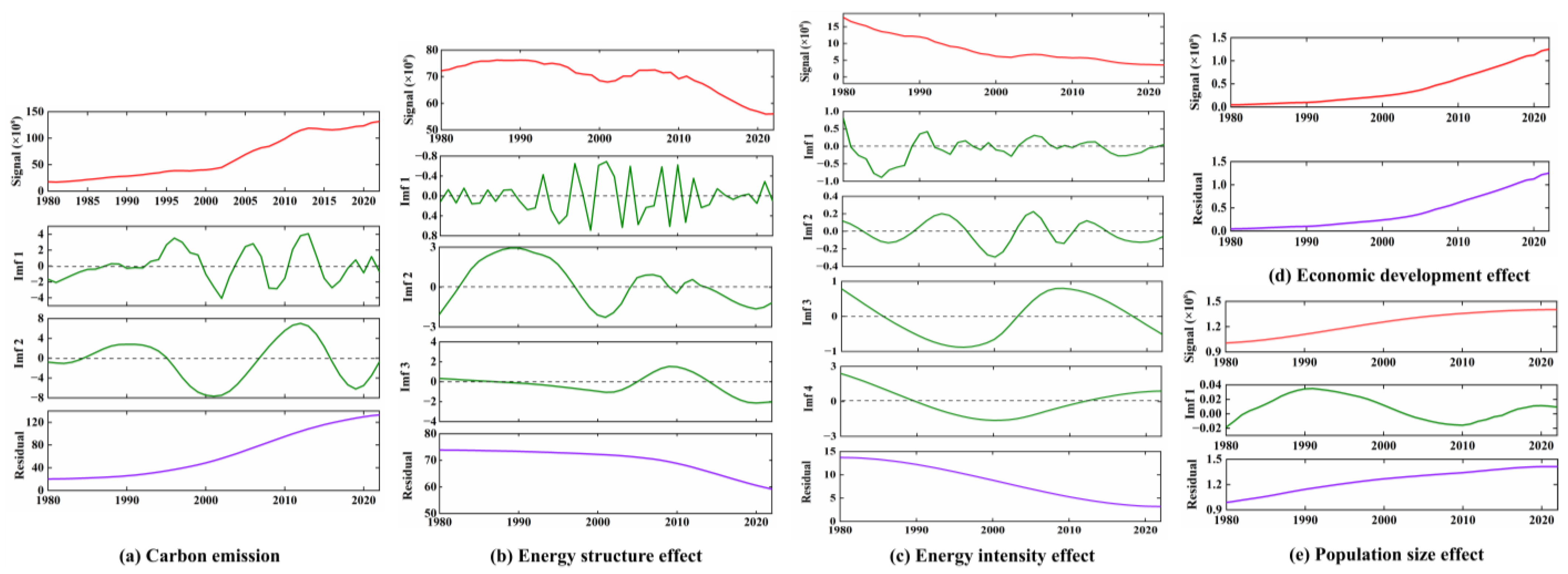
Based on the various influencing effects, this paper conducts predictive research on the changes in carbon emissions in China. The correlation between the specific quantitative indicators of each effect and carbon emissions is shown in Table 3. At the same time, to mitigate the impact of non-linearity and volatility in the data series of carbon emissions and its influencing factors on predictive accuracy, this paper employs the EMD method to preprocess the relevant data before forecasting. The specific decomposition results of the EMD are shown in Figure 6.
Table 3.
Specific quantitative indicators and relevance of each effect.
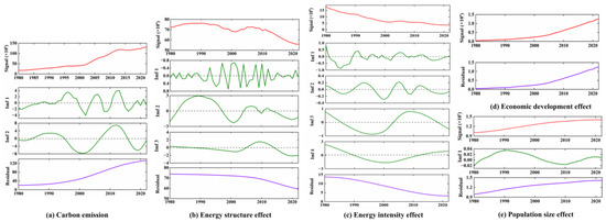
Figure 6.
EMD decomposition of carbon emissions and their influencing factors.
It is obvious that, except for the economic development effect, which shows a clear trend by itself and does not decompose the IMFs, there is non-stationarity in the carbon emissions, energy structure effect, energy intensity effect, and population size effect. Meanwhile, carbon emissions are decomposed by EMD to yield two component terms (IMF1 and IMF2) and a residual. While IMF1 displays higher-frequency fluctuations compared to IMF2, the residual indicates a continuous upward trend in carbon emissions from 1980 to 2022. The energy structure effect and energy intensity effect, on the other hand, have strong volatilities, and after EMD, the residual for both effects suggest an overall downward trend from 1980 to 2022. Regarding the intrinsic mode functions, three and four IMFs were decomposed for the energy structure effect and energy intensity effect, respectively. In both cases, IMF1 represents the highest frequency and strongest volatility. There is a weak non-stationarity in the population size effect, which is decomposed into IMF1 and a residual.
With increasing decomposition order, the frequency of components decreases, gradually approaching stability. The decomposition of EMD, carbon emissions, and influencing factors yield several intrinsic mode functions and residuals representing the respective change trends, which greatly reduces the non-stationarity of each indicator and can effectively mitigate the prediction errors associated with the volatility of the influencing factors. Indeed, the IMFs belong to high-frequency components that capture frequent oscillations, while the residual reflects the overall trend of the variable. Therefore, this paper intends to conduct separate predictions for the IMFs and residuals of carbon emissions based on the IMFs and residuals of each influencing effect.
3.2.2. The Prediction of Carbon Emissions
To effectively enhance the accuracy of carbon emission predictions, the IMFs and residuals of each effect after EMD are taken as input parameters for the LSTM models, and the prediction model is constructed separately for each IMF and residual of carbon emission after EMD. Furthermore, following an 8:2 division principle for the training and testing sets, the carbon emission data for China from 1980 to 2013 are selected as training samples, and related data from 2014 to 2022 are chosen as testing samples. To mitigate the impact of dimensionality among the indicators, normalization is initially applied to all the sets of time series data. The specific normalization formula is as follows:
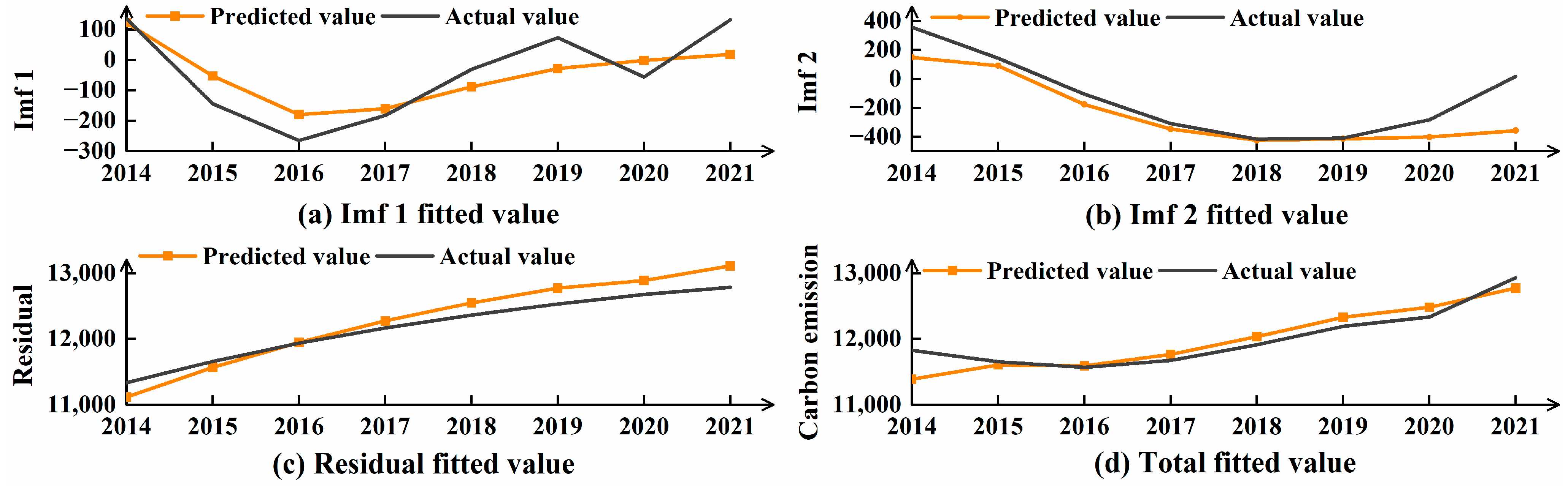
EMD of the carbon emissions results in two IMFs and one residual. This requires the establishment of three separate LSTM models, and the final sum of the prediction results will be the actual predicted value of carbon emissions. Regarding the LSTM models for predicting IMF1 and IMF2, the parameters are set as follows: the input layer dimensions are 8; the number of hidden layers is 1; the number of nodes in each hidden layer takes 8 and 7, respectively; and the dimensions of the variables in the output layer take 1. The training batch is 5, and the maximum number of iterations is 600. Moreover, to avoid overfitting the network, the dropout technique proposed by Hinton et al. [47] is introduced. The dropout rate was set to 0.2, which means that 20% of the connections between the neurons are randomly cut off. For the LSTM model predicting the residual, the parameters differ as follows: the dimension of the input layer is 4, the number of hidden layers is 1, the number of nodes in the hidden layer is 7, and the dropout rate is set to 0.2. After the EMD-LSTM model training, the predicted results for each IMF and residual from 2014 to 2022 are illustrated in Figure 7.
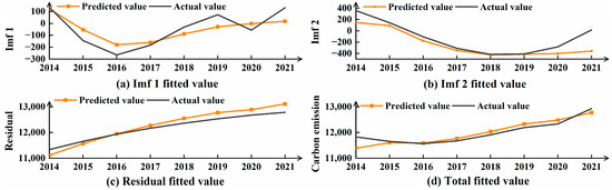
Figure 7.
LSTM prediction results for each component of carbon emissions.
By comparing the predicted curves of each component, it is observed that the fitting degree of the predicted curve for IMF1 is relatively low, indicating the poorest predictive performance. The primary reason lies in the fact that IMF1, as a high-frequency component, exhibits strong non-stationarity, making it challenging for the LSTM model to obtain precise predictions. In contrast, the volatility of IMF2 and the residual is significantly reduced, leading to better predictions for the final carbon emission values. This further underscores the effectiveness of using EMD to decompose highly volatile carbon emission data into more stable component data, substantially improving the predictive accuracy of the LSTM model.
As for the evaluation of the predictive performance of the models, this paper employs three error metrics: mean absolute error (MAE), root mean squared error (RMSE), and mean absolute percentage error (MAPE). The absolute values of MAE and RMSE may be influenced by the order of magnitude of the study objects, whereas MAPE as a percentage error circumvents this difference. The formulas for calculating each error metric are as follows:
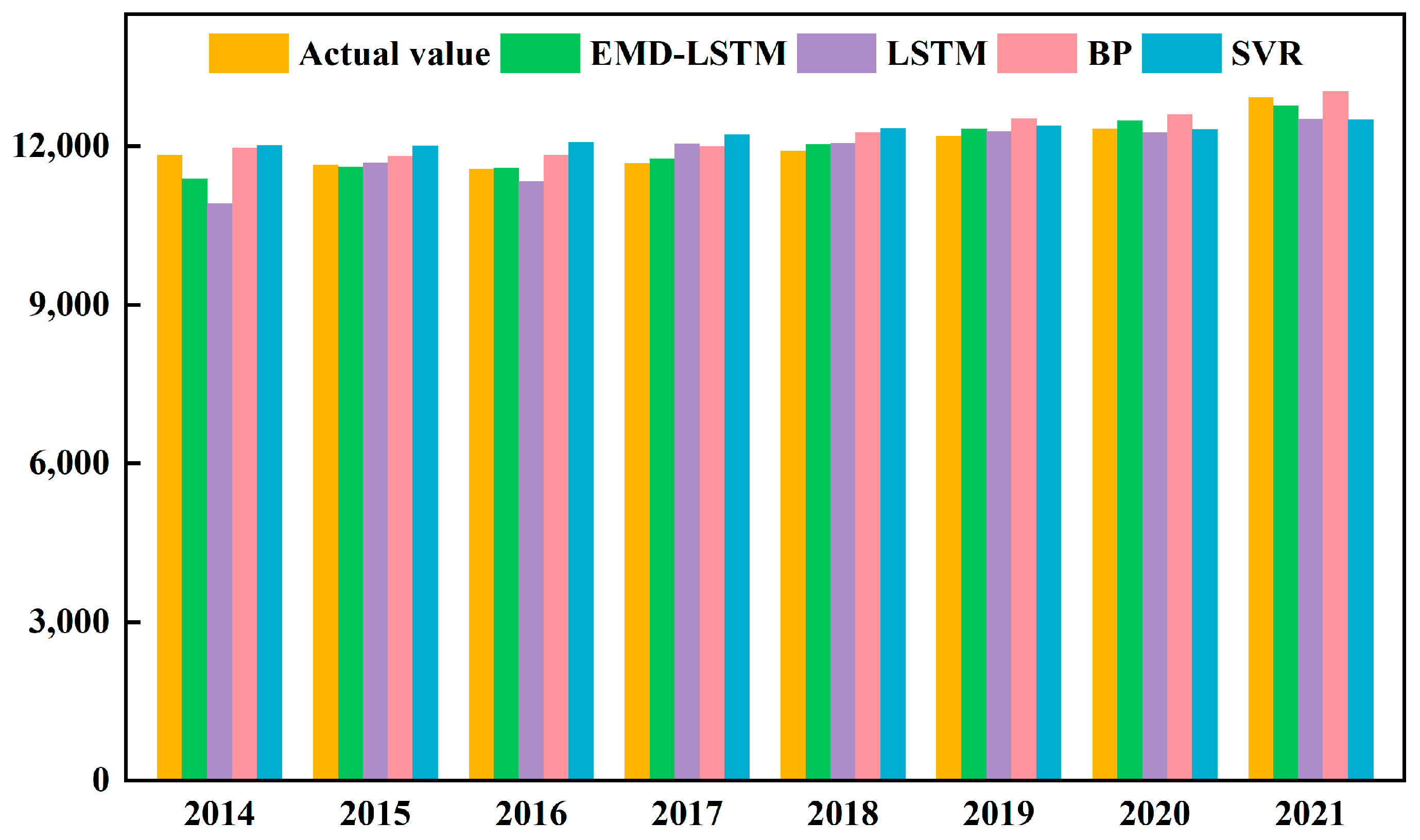
Meanwhile, to validate the superiority of the EMD-LSTM model in carbon emission prediction and the effectiveness of EMD, this paper compares it with a single model LSTM, a back propagation neural network (BPNN), and support vector regression (SVR) without EMD. The prediction results for each model are presented in Figure 8, and Table 4 illustrates the evaluation metrics for each model.

Figure 8.
Forecast results of carbon emissions in China for 2014–2022.
Table 4.
Results of error accuracy for each model.
Figure 8 and Table 4 demonstrate that the EMD-LSTM model has the best predictive performance. Its MAE, RMSE, and MAPE values are 233.50, 321.06, and 1.97%, respectively, which are significantly lower than other single models without EMD. This superiority arises from the strong volatility and nonlinearity present in the carbon emissions and the influencing factors, and decomposing them results in stable components, thereby enhancing the predictive capability of the LSTM model. Among the single models, the LSTM model has the smallest prediction error MAPE value compared to the BPNN and SVR models. However, when compared to the BP model, the EMD-LSTM model shows reductions in each error metric of 72.25, 81.46, and 0.54%.
The above results indicate that the EMD-LSTM model, by decomposing the non-stationary original sequences of carbon emissions and influencing factors into a finite number of more stable fluctuation sequences, predicts each component individually, which can effectively reduce the nonlinear and non-stationary characteristics and improve the predictive accuracy of the LSTM model.
4. Conclusions
A comprehensive model for factor decomposition and integrated prediction based on LMDI-EMD-LSTM is constructed in this paper. To effectively recognize the factors affecting carbon emissions in China, this paper adopts the LMDI method to decompose the carbon emission factors into five effects, analyzing the contribution of each influencing effect to China’s carbon emissions from 1980 to 2022. Meanwhile, to address the problem that the nonlinear and non-stationary characteristics of each sequence lead to great error in carbon emission predictions, this paper constructs an EMD-LSTM integrated model in which the EMD is first introduced into carbon emissions forecasting, decomposing the carbon emissions and their influencing factors series into fluctuation sequences with different characteristics. Finally, some benchmark models were selected for an accuracy evaluation using the established EMD-LSTM model.
The following conclusions can be drawn: (1) Economic development and population growth both contributed to increased carbon emissions, while the energy structure and intensity impacts had a negative inhibitory effect. It is unavoidable to conclude that the economic development effect and the energy intensity effect are the primary driving forces influencing China’s carbon emissions. (2) To address the non-linear and non-stationary characteristics of carbon emissions and the factors that influence them, this paper first introduces EMD into carbon emissions forecasting, which can decompose each series into fluctuation sequences with different characteristics so that the fluctuation or trend terms of different scales existing in the original series can be decomposed out. Specifically, the carbon emission data are decomposed into two IMF components and one residual, while the influencing factors are decomposed into eight IMF components and four residuals. (3) Following the decomposition using EMD, the LSTM model is constructed for carbon emission predictions. Meanwhile, the EMD-LSTM model demonstrated exceptional accuracy in predicting carbon emissions, achieving the lowest prediction error: The MAE was 233.50, the RMSE was 321.06, and the MAPE was 1.97%, which implies that using EMD to break down the non-stationary carbon emission series into more stable components can effectively enhance the accuracy of carbon emission predictions.
This paper provides a further prediction study of carbon emissions, effectively broadening the research concept of carbon emissions. Nevertheless, due to the diverse and intricate nature of the factors influencing carbon emissions, it is imperative for us to combine more methods such as random forests for factor identification. At the same time, to further strengthen the practicality of this study, we also intend to adopt other deep learning algorithms for in-depth scenario analyses based on the decomposed carbon emissions data from the EMD method.
Author Contributions
Conceptualization, Q.W. and R.S.; methodology, Q.W. and R.S.; software, Q.W.; formal analysis, Q.H.; writing—original draft Q.W. and Q.H.; writing—review and editing, R.S.; funding acquisition, R.S.; visualization, Q.H. All authors have read and agreed to the published version of the manuscript.
Funding
This work was supported by the Humanities and Social Science Fund of Ministry of Education of the People’s Republic of China (21YJA630050).
Data Availability Statement
The original data presented in this study are openly available from the Chinese National Bureau of Statistics database https://www.stats.gov.cn/sj/ndsj/, accessed on 20 March 2024.
Conflicts of Interest
The authors declare no conflicts of interest.
References
- Pan, Y.; Wang, Z.; Wang, C.; Zhang, Y. The Influence and Forecast of Three Industries and Energy Structure on Regional Carbon Emission. Energy Sources Part A Recovery Util. Environ. Eff. 2024, 46, 4078–4094. [Google Scholar] [CrossRef]
- Wang, L.; Li, Z.; Xu, Z.; Yue, X.; Yang, L.; Wang, R.; Chen, Y.; Ma, H. Carbon Emission Scenario Simulation and Policy Regulation in Resource-Based Provinces Based on System Dynamics Modeling. J. Clean. Prod. 2024, 460, 142619. [Google Scholar] [CrossRef]
- Ding, Q.; Xiao, X.; Kong, D. Estimating Energy-Related CO2 Emissions Using a Novel Multivariable Fuzzy Grey Model with Time-Delay and Interaction Effect Characteristics. Energy 2023, 263, 126005. [Google Scholar] [CrossRef]
- Liu, X.; Hu, Q.; Li, J.; Li, W.; Liu, T.; Xin, M.; Jin, Q. Decoupling Representation Contrastive Learning for Carbon Emission Prediction and Analysis Based on Time Series. Appl. Energy 2024, 367, 123368. [Google Scholar] [CrossRef]
- Li, S.; Yao, L.; Zhang, Y.; Zhao, Y.; Sun, L. China’s Provincial Carbon Emission Driving Factors Analysis and Scenario Forecasting. Environ. Sustain. Indic. 2024, 22, 100390. [Google Scholar] [CrossRef]
- Lu, F.; Ma, F.; Feng, L. Carbon Dioxide Emissions and Economic Growth: New Evidence from GDP Forecasting. Technol. Forecast. Soc. Change 2024, 205, 123464. [Google Scholar] [CrossRef]
- Du, Z.; Xu, J.; Lin, B. What does the Digital Economy bring to Household Carbon Emissions?—From the Perspective of Energy Intensity. Appl. Energy 2024, 370, 123613. [Google Scholar] [CrossRef]
- Bei, L.; Yang, W.; Wang, B.; Gao, Y.; Wang, A.; Lu, T.; Liu, H.; Sun, L. Characteristics of Residents’ Carbon Emission and Driving Factors for Carbon Peaking: A Case Study in Wuhan, China. Energy Sustain. Dev. 2024, 81, 101471. [Google Scholar] [CrossRef]
- Sun, H.; Chen, Y.; Chen, S.; Zhao, Z. Promoting the "Chinese Experience" of Carbon Neutrality—Evidence of Carbon Emission Pilot Governance in Guangdong Province based on the EIO-LCA Model. Energy Strategy Rev. 2024, 53, 101393. [Google Scholar] [CrossRef]
- Qian, W.; Zhang, H.; Sui, A.; Wang, Y. A Novel Adaptive Discrete Grey Prediction Model for Forecasting development in energy Consumption Structure—From the Perspective of Compositional Data. Grey Syst. Theory Appl. 2022, 12, 672–697. [Google Scholar] [CrossRef]
- Zhang, K.; Yin, K.; Yang, W. Predicting Bioenergy Power Generation Structure Using a Newly Developed Grey Compositional Data Model: A Case Study in China. Renew. Energy 2022, 198, 695–711. [Google Scholar] [CrossRef]
- Zhou, C.; Chen, X. Forecasting China’s Energy Consumption and Carbon Emission Based on Multiple Decomposition Strategy. Energy Strategy Rev. 2023, 49, 101160. [Google Scholar] [CrossRef]
- Tang, Y.; Zhao, Q.; Ren, Y. Nexus among Government Digital Development, Resource Dependence, and Carbon Emissions in China. Resour. Policy 2024, 95, 105186. [Google Scholar] [CrossRef]
- Wei, Y.; Wang, Z.; Wang, H.; Li, Y. Compositional Data Techniques for Forecasting Dynamic Change in China’s Energy Consumption Structure by 2020 and 2030. J. Clean. Prod. 2021, 284, 124702. [Google Scholar] [CrossRef]
- Jin, Y.; Sharifi, A.; Li, Z.; Chen, S.; Zeng, S.; Zhao, S. Carbon Emission Prediction Models: A Review. Sci. Total Environ. 2024, 927, 172319. [Google Scholar] [CrossRef] [PubMed]
- Liu, D.; Xiao, B. Can China Achieve Its Carbon Emission Peaking? A Scenario Analysis Based on STIRPAT and System Dynamics Model. Ecol. Indic. 2018, 93, 647–657. [Google Scholar] [CrossRef]
- Dietz, T.; Rosa, E.A. Effects of Population and Affluence on CO2 Emissions. Proc. Natl. Acad. Sci. USA 1997, 94, 175–179. [Google Scholar] [CrossRef] [PubMed]
- Chai, Z.; Yibo, Y.; Simayi, Z.; Shengtian, Y.; Abulimiti, M.; Yuqing, W. Carbon Emissions Index Decomposition and Carbon Emissions Prediction in Xinjiang from the Perspective of Population-Related Factors, Based on the Combination of STIRPAT Model and Neural Network. Environ. Sci. Pollut. Res. 2022, 29, 31781–31796. [Google Scholar] [CrossRef]
- Zhang, Y.; Zhang, Q.; Pan, B. Impact of Affluence and Fossil Energy on China Carbon Emissions Using STIRPAT Model. Environ. Sci. Pollut. Res. 2019, 26, 18814–18824. [Google Scholar] [CrossRef] [PubMed]
- Guo, F.; Zhang, L.; Wang, Z.; Ji, S. Research on Determining the Critical Influencing Factors of Carbon Emission Integrating GRA with an Improved Stirpat Model: Taking the Yangtze River Delta as an Example. Int. J. Environ. Res. Public Health 2022, 19, 8791. [Google Scholar] [CrossRef]
- Li, X.; Lin, C.; Lin, M.; Jim, C.Y. Drivers and Spatial Patterns of Carbon Emissions from Residential Buildings: An Empirical Analysis of Fuzhou City (China). Build. Environ. 2024, 257, 111534. [Google Scholar] [CrossRef]
- Xiao, B.; Niu, D.; Wu, H. Exploring the Impact of Determining Factors Behind CO2 Emissions in China: A CGE Appraisal. Sci. Total Environ. 2017, 581–582, 559–572. [Google Scholar] [CrossRef] [PubMed]
- Li, J.; Ma, Z.; Sun, H.; Chen, W. Driving Factor Analysis and Dynamic Forecast of Industrial Carbon Emissions in Resource-Dependent Cities: A Case Study of Ordos, China. Environ. Sci. Pollut. Res. 2023, 30, 92146–92161. [Google Scholar] [CrossRef]
- Ma, H.; Liu, J.; Xi, J. Decoupling and Decomposition Analysis of Carbon Emissions in Beijing’s Tourism Traffic. Environ. Dev. Sustain. 2021, 24, 5258–5274. [Google Scholar] [CrossRef]
- Hao, J.; Gao, F.; Fang, X.; Nong, X.; Zhang, Y.; Hong, F. Multi-Factor Decomposition and Multi-Scenario Prediction Decoupling Analysis of China’s Carbon Emission under Dual Carbon Goal. Sci. Total Environ. 2022, 841, 156788. [Google Scholar] [CrossRef] [PubMed]
- Zhang, Q.; Li, J. Building Carbon Peak Scenario Prediction in China Using System Dynamics Model. Environ. Sci. Pollut. Res. 2023, 30, 96019–96039. [Google Scholar] [CrossRef] [PubMed]
- Peng, D.; Liu, H. Measurement and Driving Factors of Carbon Emissions from Coal Consumption in China Based on the Kaya-Lmdi Model. Energies 2022, 16, 439. [Google Scholar] [CrossRef]
- Wang, Z.-X.; Ye, D.-J. Forecasting Chinese Carbon Emissions from Fossil Energy Consumption Using Non-Linear Grey Multivariable Models. J. Clean. Prod. 2017, 142, 600–612. [Google Scholar] [CrossRef]
- Wang, Q.; Li, S.; Pisarenko, Z. Modeling Carbon Emission Trajectory of China, Us and India. J. Clean. Prod. 2020, 258, 120723. [Google Scholar] [CrossRef]
- Ma, X.; Han, M.; Luo, J.; Song, Y.; Chen, R.; Sun, X. The Empirical Decomposition and Peak Path of China’s Tourism Carbon Emissions. Environ. Sci. Pollut. Res. 2021, 28, 66448–66463. [Google Scholar] [CrossRef] [PubMed]
- Ye, L.; Yang, D.; Dang, Y.; Wang, J. An Enhanced Multivariable Dynamic Time-Delay Discrete Grey Forecasting Model for Predicting China’s Carbon Emissions. Energy 2022, 249, 123681. [Google Scholar] [CrossRef]
- Luo, X.; Liu, C.; Zhao, H. Driving Factors and Emission Reduction Scenarios Analysis of CO2 Emissions in Guangdong-Hong Kong-Macao Greater Bay Area and Surrounding Cities Based on Lmdi and System Dynamics. Sci. Total Environ. 2023, 870, 161966. [Google Scholar] [CrossRef] [PubMed]
- Rao, C.; Huang, Q.; Chen, L.; Goh, M.; Hu, Z. Forecasting the Carbon Emissions in Hubei Province under the Background of Carbon Neutrality: A Novel Stirpat Extended Model with Ridge Regression and Scenario Analysis. Environ. Sci. Pollut. Res. 2023, 30, 57460–57480. [Google Scholar] [CrossRef] [PubMed]
- Fang, D.; Zhang, X.; Yu, Q.; Jin, T.C.; Tian, L. A Novel Method for Carbon Dioxide Emission Forecasting Based on Improved Gaussian Processes Regression. J. Clean. Prod. 2018, 173, 143–150. [Google Scholar] [CrossRef]
- Zhu, B.; Ye, S.; Jiang, M.; Wang, P.; Wu, Z.; Xie, R.; Chevallier, J.; Wei, Y.-M. Achieving the Carbon Intensity Target of China: A Least Squares Support Vector Machine with Mixture Kernel Function Approach. Appl. Energy 2019, 233–234, 196–207. [Google Scholar] [CrossRef]
- Niu, D.; Wang, K.; Wu, J.; Sun, L.; Liang, Y.; Xu, X.; Yang, X. Can China Achieve Its 2030 Carbon Emissions Commitment? Scenario Analysis Based on an Improved General Regression Neural Network. J. Clean. Prod. 2020, 243, 118558. [Google Scholar] [CrossRef]
- Chen, J.; Yu, J.; Song, M.; Valdmanis, V. Factor Decomposition and Prediction of Solar Energy Consumption in the United States. J. Clean. Prod. 2019, 234, 1210–1220. [Google Scholar] [CrossRef]
- Wang, Q.; Suo, R.; Han, Q. A Study on Natural Gas Consumption Forecasting in China Using the LMDI-PSO-LSTM Model: Factor Decomposition and Scenario Analysis. Energy 2024, 292, 130435. [Google Scholar] [CrossRef]
- Huang, Y.; Shen, L.; Liu, H. Grey Relational Analysis, Principal Component Analysis and Forecasting of Carbon Emissions Based on Long Short-Term Memory in China. J. Clean. Prod. 2019, 209, 415–423. [Google Scholar] [CrossRef]
- Shi, C.; Zhi, J.; Yao, X.; Zhang, H.; Yu, Y.; Zeng, Q.; Li, L.; Zhang, Y. How can China Achieve the 2030 Carbon Peak Goal—A Crossover Analysis Based on Low-Carbon Economics and Deep Learning. Energy 2023, 269, 126776. [Google Scholar] [CrossRef]
- Yousaf Raza, M.; Lin, B. Development Trend of Pakistan’s Natural Gas Consumption: A Sectorial Decomposition Analysis. Energy 2023, 278, 127872. [Google Scholar] [CrossRef]
- Ang, B.W. The LMDI Approach to Decomposition Analysis: A Practical Guide. Energy Policy 2005, 33, 867–871. [Google Scholar] [CrossRef]
- Huang, N.E.; Shen, Z.; Long, S.R.; Wu, M.C.; Shih, H.H.; Zheng, Q.; Yen, N.-C.; Tung, C.C.; Liu, H.H. The Empirical Mode Decomposition and the Hilbert Spectrum for Nonlinear and Non-Stationary Time Series Analysis. Proc. Math. Phys. Eng. Sci. 1998, 454, 903–995. [Google Scholar] [CrossRef]
- Cang, D.; Chen, C.; Chen, Q.; Lili, S.; Caiyun, C. Does New Energy Consumption Conducive to Controlling Fossil Energy Consumption and Carbon Emissions?-Evidence from China. Resour. Policy 2021, 74, 102427. [Google Scholar] [CrossRef]
- Wang, Y.; Zhou, Y.; Zhu, L.; Zhang, F.; Zhang, Y. Influencing Factors and Decoupling Elasticity of China’s Transportation Carbon Emissions. Energies 2018, 11, 1157. [Google Scholar] [CrossRef]
- Ji, J.; Li, C.; Ye, X.; Song, Y.; Lv, J. Analysis of the Spatial and Temporal Evolution of China’s Energy Carbon Emissions, Driving Mechanisms, and Decoupling Levels. Sustainability 2023, 15, 15843. [Google Scholar] [CrossRef]
- Hinton, G.E.; Srivastava, N.; Krizhevsky, A.; Sutskever, I.; Salakhutdinov, R.R. Improving Neural Networks by Preventing Co-Adaptation of Feature Detectors. arXiv 2012, arXiv:1207.0580. [Google Scholar]
Disclaimer/Publisher’s Note: The statements, opinions and data contained in all publications are solely those of the individual author(s) and contributor(s) and not of MDPI and/or the editor(s). MDPI and/or the editor(s) disclaim responsibility for any injury to people or property resulting from any ideas, methods, instructions or products referred to in the content. |
© 2024 by the authors. Licensee MDPI, Basel, Switzerland. This article is an open access article distributed under the terms and conditions of the Creative Commons Attribution (CC BY) license (https://creativecommons.org/licenses/by/4.0/).