Optimal Investment Consumption Choices under Mispricing and Habit Formation

Abstract

This paper studies the optimal consumption and investment for an agent, considering statistical arbitrary opportunities caused by mispriced stocks. The agent exhibits consumption habit formation and has access to a risk-free asset, a market index, and a pair of mispriced stocks. The optimization problem is to find the optimal consumption and investment strategies to maximize the expected utility from consumption and terminal wealth. The utility of consumption stems from the difference between the consumption and habit levels. Based on the dynamic programming method, a verification theorem is provided, and the analytical solution of the optimization problem is obtained. The numerical results show the behaviors of our formulas and are used to make practical recommendations. By studying the sensitivity of consumption and investment strategies to habit formation, mispricing, and a delta-neutral arbitrage strategy, we uncover and analyze the behaviors of the agent. Meanwhile, we define and discuss the wealth-equivalent utility loss in three cases, including ignoring habit formation, ignoring mispricing, and adopting the delta-neutral arbitrage strategy.

1. Introduction

Research on investment and consumption has always been a hot topic in the field of financial mathematics. Since Ref. [1] first set up and solved an investment consumption problem in the context of continuous time, there has a surge in relevant literature, such as [2,3,4,5], and so on. These works all study the optimal asset allocation in the context of the financial market involving one or multi-risk assets, and they explore the effects of market features on the optimal strategies, where the market features include the stochastic volatility risk of the risky assets, inflation risks, and stochastic rate risks. However, in the real financial market, there exists a so-called mispricing phenomenon.

Mispricing is a price difference between a pair of assets, where two assets with identical or nearly identical contingent claim values should have the same or close to the same price during the same trading period Ref. [6]. The main reason for this kind of phenomenon is the friction caused by the immaturity of the financial market. Usually, such assets do not have the same or nearly the same price in different financial markets. For example, there exists mispricing in some Chinese company stocks (such as Bank of China, Agriculture Bank of China, and others) traded on both Chinese stock exchanges as share A and Hong Kong stock exchanges as share H. Ref. [6] points out that since 2015, the Chinese government has opened up simultaneous investment in the Hong Kong and mainland China financial markets, which means that a mainland China investor is allowed to invest in designated Hong Kong stocks and vice versa. Therefore, this work is of timely significance to Chinese investors. If an investor applies the pairs trading strategy to the mispricing stock pairs, the market systemic risk will be hedged to some extent. Ref. [7] obtains the optimal long–short investment strategy, which is an arbitrage opportunity caused by mispricing assets. After that, the optimal asset allocation problem with mispricing has followed with interest. Ref. [8] shows that conventional long–short delta-neutral strategies are generally suboptimal, and it can be optimal to simultaneously go long (or short) in two mispriced assets. Under a utility function framework, based on Refs. [8,9], we find that mispricing has an effect on the optimal portfolio selection. Ref. [6] shows that the mispricing feature causes statistical arbitrage opportunities, which are particularly timely in the investment environment for markets in mainland China and Hong Kong. Ref. [10] discloses that liquidity has an important role in the so-called long–short (L-S) strategy, which corresponds to statistical arbitrage afforded by mispricing. To the best of our knowledge, the existing literature involving investment and consumption does not consider mispricing; thus, we introduce it in this paper.

In addition to the mispricing phenomenon, the formation of consumption habits is attracting the attention of more scholars. Ref. [11] uncovered that models with habit formation can obtain a high equity premium with low-risk aversion and thus used habit formation to explain the equity premium puzzle. Afterwards, in the context of time-separable power utility, Ref. [12] provided empirical support for this result. Ref. [13] suggests that the utility associated with the consumption choice should depend on past consumption choices. Ref. [14] showed that it is unrealistic if one assumes that current satisfaction only relies on current consumption. Ref. [15] showed that the existence of habit formation affects the optimal decision of the agent. Thus, in a more reasonable preference expression, one should consider the formation of consumption habits.

However, the above work either considers mispricing without considering the formation of the agent’s consumption habits in the context of investment portfolio framework, such as Refs. [6,7,8,9,10], or it only considers the formation of consumption habits without considering mispricing phenomena, such as Refs. [11,12,13,14,15]. To the best of our knowledge, we are the first to simultaneously consider the mispricing phenomenon and habit formation in a consumption investment problem. The second contribution is that we provide a verification theorem and obtain closed-form expressions of optimal consumption investment strategies and the optimal value function for the agent who ignores mispricing and for the agent who takes the delta-neutral arbitrage strategy for granted.

The third contribution of this paper is that, based on a numerical analysis, we show the effects of mispricing and habit formation on the optimal strategy. Specifically, this paper considers six cases of the model. That is, the case involving mispricing and habit formation, the case involving the delta-neutral strategy and habit formation, the case involving mispricing and no habit formation, the case involving the delta-neutral strategy and no habit formation, the case without mispricing but involving habit formation, and the case without mispricing or habit formation. Detailed results are also provided. (i) For a longer time horizon, when considering mispricing or the delta-neutral strategy, habit formation damps consumption. However, habit formation increases consumption when ignoring mispricing, and taking the delta-neutral strategy diminishes consumption. For a shorter time horizon, consumption increases with time t, and the effects of habit formation and mispricing on consumption gradually disappear. (ii) Habit formation decreases the portfolio weights of wealth invested in the market index, while ignoring mispricing or adopting the delta-neutral strategy will raise it. Meanwhile, the results show that there is almost no difference between ignoring mispricing and adopting the delta-neutral strategy when investing in the market index. (iii) As the time horizon shortens, the portfolio weights of wealth invested in the pair of mispriced stocks decrease. (iv) We respectively define and analyze the wealth-equivalent utility loss under three cases, including ignoring habit formation, ignoring mispricing, and adopting the delta-neutral arbitrage strategy. When considering mispricing, habit formation dampens consumption, leading to the agent’s utility (from consumption) decreasing. Thus, if one ignores habit formation, the utility will increase. In addition, ignoring mispricing or adopting the delta-neutral arbitrage strategy will lead to utility loss.

The remainder of this study is organized as follows: Section 2 introduces some necessary assumptions and formulates the model. Section 3 solves the optimal consumption and investment problem with mispricing and consumption habits. Section 4 shows numerical results used to analyze the sensitivity of consumption and investment strategies to some parameters. Section 5 concludes this paper.

2. Model Formulation

This section sets up a continuous time investment and consumption model. Assume that an agent can trade in the financial market with no transaction costs or taxes. Let $T>0$ be a fixed constant as the time horizon and $(\Omega ,\mathcal{F},\{\mathcal{F}\left(t\right)\},P)$ be a complete probability space. $\left\{\mathcal{F}\right(t\left)\right\}$ is the natural filtration, and it satisfies the usual conditions (i.e., $\left\{\mathcal{F}\right(t\left)\right\}$ is P-complete and right-continuous). $\mathcal{F}\left(t\right)$ represents the information available until time t. All the stochastic processes and random variables introduced below are supposed to be well-defined and adapted to $\left\{\mathcal{F}\right(t\left)\right\}$.

2.1. The Financial Market

Assume that the financial market in our model consists of one risk-free asset, one market index, and a pair of stocks with mispricing. The price process of the risk-free asset, denoted by $S_0\left(t\right)$, satisfies the following ordinary differential equation:

$$\begin{array}{c}\hfill {\displaystyle \frac{\mathrm{d}{S}_0\left(t\right)}{S_0\left(t\right)}}=r\mathrm{d}t,\end{array}$$

(1)

where $r>0$ is the risk-free interest rate. The price process of the market index, $S_m\left(t\right)$, reflects the market performance and follows geometric Brownian motion:

$$\begin{array}{c}\hfill {\displaystyle \frac{\mathrm{d}{S}_m\left(t\right)}{S_m\left(t\right)}}=(r+{\mu }_m)\mathrm{d}t+{\sigma }_m\mathrm{d}B\left(t\right),\end{array}$$

(2)

where ${\mu }_m$ is the market risk premium, ${\sigma }_m>0$ is the market volatility, and $\left\{B\right(t\left)\right\}$ is standard Brownian motion. Let $S_1\left(t\right)$ and $S_2\left(t\right)$ denote mispriced price process of the pair of stocks and satisfy the following stochastic differential equations:

$$\begin{array}{c}\hfill \begin{array}{c}\hfill {\displaystyle \frac{\mathrm{d}{S}_1\left(t\right)}{S_1\left(t\right)}}=(r+{\mu }_m\beta )\mathrm{d}t+\beta {\sigma }_m\mathrm{d}B\left(t\right)+\sigma \mathrm{d}Z\left(t\right)+b\mathrm{d}{Z}_1\left(t\right)-l_{1}X\left(t\right)\mathrm{d}t,\\ \hfill {\displaystyle \frac{\mathrm{d}{S}_2\left(t\right)}{S_2\left(t\right)}}=(r+{\mu }_m\beta )\mathrm{d}t+\beta {\sigma }_m\mathrm{d}B\left(t\right)+\sigma \mathrm{d}Z\left(t\right)+b\mathrm{d}{Z}_2\left(t\right)+l_{2}X\left(t\right)\mathrm{d}t,\end{array}\end{array}$$

(3)

where $l_1, l_2, \sigma , b$, and $\beta$ are constants. The term $\beta {\sigma }_m\mathrm{d}B\left(t\right)$ is the systematic risk of the market, $\sigma \mathrm{d}Z\left(t\right)+b\mathrm{d}{Z}_i\left(t\right)(i=1,2)$ is the idiosyncratic risk of the stock, $\sigma \mathrm{d}Z\left(t\right)$ describes the common risk, and $b\mathrm{d}{Z}_i\left(t\right)$ is the individual risk. $Z\left(t\right),Z_1\left(t\right)$ and $Z_2\left(t\right)$ are mutually independent Brownian motions and are both independent of $B\left(t\right)$. $X\left(t\right)=ln{S}_1\left(t\right)-ln{S}_2\left(t\right)$ denotes the pricing error or mispricing between two stocks. Then, $l_{i}X\left(t\right)$ describes the effects of mispricing on the ith stock. Meanwhile, based on the $\mathrm{It}\widehat{\mathrm{o}}$ formula, the dynamics of the pricing error $X\left(t\right)$ can be given.

$$\begin{array}{c}\hfill \mathrm{d}X\left(t\right)=(l_1+l_2)(0-X\left(t\right))\mathrm{d}t+b\mathrm{d}{Z}_1\left(t\right)-b\mathrm{d}{Z}_2\left(t\right),X\left(0\right)=x_0.\end{array}$$

(4)

It is easy to see that $X\left(t\right)$ is a Gaussian mean reverting process; the long-run mean of $X\left(t\right)$ is 0, and the mean reversion rate of it is $l_1+l_2$. In Equation (4), $l_1$ and $l_2$ cannot equal zero at the same time; otherwise, there is no pricing error. Assume $l_1+l_2>0$ to assure that $X\left(t\right)$ is stationary (cf. [6,8,9]). Sometimes, we can view $l_1$ and $l_2$ as liquidities, while inadequate liquidities may cause market frictions, which give rise to mispricing. As described in Ref. [6], when $l_1$ and $l_2$ are low, a mispricing process $X\left(t\right)$ will take longer to go back to the zero mean. This is consistent with the prevailing view that more friction accompanies high illiquidity.

2.2. Consumption Habits and Wealth Process

Assume that the agent exhibits consumption habit formation. Let $h\left(t\right)$ be the habit level at time t and satisfy the following:

$$\begin{array}{c}\hfill h\left(t\right)=h_0{\mathrm{e}}^{-{\xi }_{2}t}+{\xi }_1{\int }_0^t{\mathrm{e}}^{-{\xi }_2(t-s)}c\left(s\right)\mathrm{d}s\end{array}$$

(5)

or

$$\begin{array}{c}\hfill \mathrm{d}h\left(t\right)=({\xi }_{1}c\left(t\right)-{\xi }_{2}h\left(t\right))\mathrm{d}t,\end{array}$$

(6)

where $h\left(0\right)=h_0(>0)$, ${\xi }_1(>0)$ and ${\xi }_2(>0)$ are the initial habit level, the scaling parameter, and the persistence parameter, respectively. ${\xi }_1$ measures the intensity of the consumption habit, which means that as ${\xi }_1$ increases, the habit has an emphasis on the past consumption. ${\xi }_2$ measures the persistence of past consumption. $c\left(s\right)$ is the consumption rate at time t. Similar to Refs. [13,14,15,16], we let ${\xi }_2>{\xi }_1$ ensure that the habit level will decay when the consumption rate is in line with the habit level. In this sense, given $h\left(t\right)$, from time t onwards, if the agent’s consumption is exactly at the minimum, that is $c\left(s\right)=h\left(s\right)$ for $s\ge t$, then the future habit level is given by the following:

$$\begin{array}{c}\hfill h\left(s\right)=h\left(t\right){\mathrm{e}}^{-({\xi }_2-{\xi }_1)(s-t)},\mathrm{for}s\ge t.\end{array}$$

(7)

Equation (7) shows the minimum consumption level of the agent. Noticed that when ${\xi }_2-{\xi }_1$ is small, the consumption habit only descends very slowly, even with minimum consumption. Thus, it restricts the agent more (see Ref. [17]), and the larger (smaller) ${\xi }_2-{\xi }_1$ value indicates weaker (stronger) consumption habit strengths. In other words, ${\xi }_2-{\xi }_1$ depicts the consumption habit strength by determining to what extent the current level of the habit limits future consumption choices. This implies that the agent is motivated to smooth his/her consumption, suggests that past consumption has a significant impact on current and future economic decisions, and reflects the psychological rationality of the agent.

Again, assume that in the horizon $[0,T]$, from the non-financial market, the agent obtains a stream of income at a rate of $Y\left(t\right)$. The dynamics of $Y\left(t\right)$ satisfy the following:

$$\begin{array}{c}\hfill \mathrm{d}Y\left(t\right)={\mu }_{Y}Y\left(t\right)\mathrm{d}t,\end{array}$$

(8)

where ${\mu }_Y>0$ is the growth rate of income.

Let ${\pi }_m\left(t\right),{\pi }_1\left(t\right)$, and ${\pi }_2\left(t\right)$ be the portfolio weights of wealth invested in the market index and the pair of mispriced stocks. Then, $1-{\pi }_m\left(t\right)-{\pi }_1\left(t\right)-{\pi }_2\left(t\right)$ is the proportion of wealth invested in the risk-free asset. Denote $\pi =\{({\pi }_m\left(t\right),{\pi }_1\left(t\right),{\pi }_2\left(t\right)):0\le t\le T\}$, then the wealth process $W\left(t\right)$ can be given by the following:

$$\begin{array}{cc}\hfill \mathrm{d}W\left(t\right)=& (1-{\pi }_m\left(t\right)-{\pi }_1\left(t\right)-{\pi }_2\left(t\right))rW\left(t\right)\mathrm{d}t+{\pi }_m\left(t\right)W\left(t\right){\displaystyle \frac{\mathrm{d}{S}_m\left(t\right)}{S_m\left(t\right)}}\hfill \\ \hfill & +{\pi }_1\left(t\right)W\left(t\right){\displaystyle \frac{\mathrm{d}{S}_1\left(t\right)}{S_1\left(t\right)}}+{\pi }_2\left(t\right)W\left(t\right){\displaystyle \frac{\mathrm{d}{S}_2\left(t\right)}{S_2\left(t\right)}}+Y\left(t\right)\mathrm{d}t-c\left(t\right)\mathrm{d}t\hfill \\ \hfill =& W\left(t\right)\left(r+{\mu }_m{\widehat{\pi }}_m\left(t\right)-l_1{\pi }_1\left(t\right)X\left(t\right)+l_2{\pi }_2\left(t\right)X\left(t\right)\right)\mathrm{d}t+Y\left(t\right)\mathrm{d}t-c\left(t\right)\mathrm{d}t\hfill \\ \hfill & +W\left(t\right){\sigma }_m{\widehat{\pi }}_m\left(t\right)\mathrm{d}B\left(t\right)+W\left(t\right)\left({\pi }_1\left(t\right)+{\pi }_2\left(t\right)\right)\sigma \mathrm{d}Z\left(t\right)\hfill \\ \hfill & +W\left(t\right){\pi }_1\left(t\right)b\mathrm{d}{Z}_1\left(t\right)+W\left(t\right){\pi }_2\left(t\right)b\mathrm{d}{Z}_2\left(t\right),\hfill \end{array}$$

(9)

where

$$\begin{array}{c}\hfill {\widehat{\pi }}_m\left(t\right)={\pi }_m\left(t\right)+\beta ({\pi }_1\left(t\right)+{\pi }_2\left(t\right)).\end{array}$$

(10)

2.3. Optimization Problem

Definition 1

(Admissible Strategy). A consumption and investment processes pair $(c,\pi ):=\left\{c\right(t),\pi (t\left)\right\}$ is said to be admissible if it satisfies the following:

(1) $\left\{c\right(t\left)\right\}$ and $\left\{\pi \right(t\left)\right\}$ are adapted to $\left\{\mathcal{F}\right(t\left)\right\}$, $\forall t\in [0,T]$;

(2) $\mathbb{E}\left[{\int }_0^{T}c\left(t\right)\mathrm{d}t\right]<\infty ,\mathbb{E}[{\int }_0^{T}W{\left(t\right)}^2{\Vert \pi \left(t\right)\Vert }^2\mathrm{d}t]<\infty$, where $\Vert ·\Vert$ denotes the Euclidean norm of a vector.

(3) Equation (9) has a pathwise unique strong solution for $\forall (t,w,x,y,h)\in [0,T]\times \mathcal{R}\times \mathcal{R}\times {\mathcal{R}}^{+}\times {\mathcal{R}}^{+}$.

Let Π denote the set of all admissible strategies.

Now, the optimization problems of the agent is to seek a strategy $(c,\pi )\in \Pi$ to maximize the expected utility as follows:

$$\begin{array}{c}\hfill \underset{(c,\pi )\in \Pi }{max}\mathbb{E}\left[{\int }_0^T{\mathrm{e}}^{-\rho s}{U}_1(c\left(s\right)-h\left(s\right))\mathrm{d}s+{\mathrm{e}}^{-\rho T}\epsilon U_2\left(W\left(T\right)\right)\right],\end{array}$$

(11)

where $\rho$ is the time preference; $\epsilon$ describes the individual’s weight relative to the utility of terminal wealth; and $U_1(·)$ and $U_2(·)$ are strictly increasing, strictly concave, and continuously differentiable utility functions with the following forms:

$$\begin{array}{c}\hfill U_i^{\prime }(0+)=\underset{x\to 0+}{lim}{U}_i^{\prime }\left(x\right)=\infty ,U_i^{\prime }(\infty )=\underset{x\to \infty }{lim}{U}_i^{\prime }\left(x\right)=0.\end{array}$$

(12)

Equation (11) shows that the agent obtains utility from the following two aspects: $c\left(t\right)-h\left(t\right)$, the difference between the consumption $c\left(t\right)$ and habit level $h\left(t\right)$; and $W\left(T\right)$, the terminal wealth. Let $\Pi \left(t\right)$ be the set of all admissible strategies over time interval $[t,T]$. We define the value function at time t as follows:

$$\begin{array}{cc}\hfill V(t,w,x,y,h)& =\underset{(c,\pi )\in \Pi \left(t\right)}{max}\mathbb{E}\left[{\int }_t^T{\mathrm{e}}^{-\rho (s-t)}{U}_1(c\left(s\right)-h\left(s\right))\mathrm{d}s+{\mathrm{e}}^{-\rho (T-t)}\epsilon U_2\left(W\left(T\right)\right)\right],\hfill \end{array}$$

(13)

where ${\mathbb{E}}_t[·]={\mathbb{E}}_t[·|W\left(t\right)=w,X\left(t\right)=x,Y\left(t\right)=y,h\left(t\right)=h]$.

3. Solution of the Optimization Problems

To reduce the complexity of the model, suppose that the utility functions have the following expression (cf. [15]):

$$\begin{array}{c}\hfill U_i\left(x\right)={\displaystyle \frac{x^{1-\gamma }}{1-\gamma }}:=U\left(x\right),i=1,2,\end{array}$$

(14)

where $\gamma (\gamma >0,\gamma \ne 1)$ is the relative risk aversion coefficient. Under the power utility function, we solve optimization (13). Moreover, we show two special cases by imposing special values for some parameters.

3.1. Optimal Consumption and Investment Strategies

For convenience, we introduce $C^{1,2,2,1,1}:=C^{1,2,2,1,1}([0,T]\times \mathbb{R}\times \mathbb{R}\times {\mathbb{R}}^{+}\times {\mathbb{R}}^{+})=\left\{\phi \right(t,w,x,y,$$h):\phi (t,·,·,y,h)$, which is once continuously differentiable for t on $[0,T]$, y on ${\mathbb{R}}^{+}$, and h on ${\mathbb{R}}^{+}$. $\phi (·,w,x,·,·)$ is twice continuously differentiable for w on $\mathbb{R}$ and x on $\mathbb{R}\}$. For any function $\phi (t,w,x,y,h)\in C^{1,2,2,1,1}$, we define a differential operator:

$$\begin{array}{cc}\hfill & {\mathcal{A}}^{c,\pi }\phi (t,w,x,y,h)=-\rho \phi +{\phi }_t+\left(rw+y-c+{\mu }_{m}w{\widehat{\pi }}_m-l_{1}xw{\pi }_1+l_{2}xw{\pi }_2\right){\phi }_w\hfill \\ \hfill & +({\xi }_{1}c-{\xi }_{2}h){\phi }_h+{\mu }_{Y}y{\phi }_y-(l_1+l_2)x{\phi }_x+{\displaystyle \frac{1}{2}}({\sigma }_m^2{\widehat{\pi }}_m^2+{\sigma }^2{({\pi }_1+{\pi }_2)}^2\hfill \\ \hfill & +b^2({\pi }_1^2+{\pi }_2^2))w^2{\phi }_{ww}+b^2{\phi }_{xx}+b^2({\pi }_1-{\pi }_2)w{\phi }_{wx}\hfill \end{array}$$

(15)

where ${\phi }_t,{\phi }_w,{\phi }_x,{\phi }_y,{\phi }_h,{\phi }_{ww},{\phi }_{xx}$, and ${\phi }_{wx}$ represent the partial derivatives of $\phi (t,w,x,y,h)$ with respect to (w.r.t.) the corresponding variables.

Based on the principle of stochastic dynamic programming, the corresponding Hamilton–Jacobi–Bellman (HJB) equation of the value function (13) can be given as follows:

$$\begin{array}{c}\hfill \underset{(c,\pi )\in \Pi \left(t\right)}{max}\left\{{\mathcal{A}}_1^{c,\pi }V(t,w,x,y,h)+U(c-h)\right\}=0\end{array}$$

(16)

with the boundary condition $V(T,w,x,y,h)=\epsilon U\left(w\right)$.

In order to solve (16), suppose that $J(t,h,w,x,y)$ is a solution of (16) and satisfies the first-order optimal conditions as follows:

$$\begin{array}{cc}\hfill c^{*}& =h+{\left(1-{\xi }_1{\displaystyle \frac{J_h}{J_w}}\right)}^{-{\displaystyle \frac{1}{\gamma }}}{J}_w^{-{\displaystyle \frac{1}{\gamma }}},\hfill \end{array}$$

(17)

$$\begin{array}{cc}\hfill {\widehat{\pi }}_m^{*}& =-{\displaystyle \frac{{\mu }_m}{{\sigma }_m^2}}{\displaystyle \frac{J_w}{w{J}_{ww}}},\hfill \end{array}$$

(18)

$$\begin{array}{cc}\hfill {\pi }_1^{*}& ={\displaystyle \frac{\left({\sigma }^2(l_1+l_2)+b^2{l}_1\right)x{J}_w}{b^2(2{\sigma }^2+b^2)w{J}_{ww}}}-{\displaystyle \frac{J_{wx}}{w{J}_{ww}}},\hfill \end{array}$$

(19)

$$\begin{array}{cc}\hfill {\pi }_2^{*}& =-{\displaystyle \frac{\left({\sigma }^2(l_1+l_2)+b^2{l}_2\right)x{J}_w}{b^2(2{\sigma }^2+b^2)w{J}_{ww}}}+{\displaystyle \frac{J_{wx}}{w{J}_{ww}}}.\hfill \end{array}$$

(20)

Substituting (17)–(20) into (16) results in the following:

$$\begin{array}{cc}{\displaystyle \frac{\gamma }{1-\gamma }}\hfill & {\left(1-{\xi }_1{\displaystyle \frac{J_h}{J_w}}\right)}^{{\displaystyle \frac{\gamma -1}{\gamma }}}{J}_w^{{\displaystyle \frac{\gamma -1}{\gamma }}}-{\displaystyle \frac{{\mu }_m^2}{2{\sigma }_m^2}}{\displaystyle \frac{J_w^2}{J_{ww}}}+(l_1+l_2){\displaystyle \frac{x{J}_w{J}_{wx}}{J_{ww}}}-b^2{\displaystyle \frac{J_{wx}^2}{J_{ww}}}\hfill \\ \hfill -& {\displaystyle \frac{{\sigma }^2{(l_1+l_2)}^2+b^2(l_1^2+l_2^2)}{2b^2(2{\sigma }^2+b^2)}}{\displaystyle \frac{x^2{J}_w^2}{J_{ww}}}+J_t+(rw+y-h)J_w+b^2{J}_{xx}\hfill \\ \hfill -& (l_1+l_2)x{J}_x+{\mu }_{Y}y{J}_y+({\xi }_1-{\xi }_2)h{J}_h-\rho J=0.\hfill \end{array}$$

(21)

We try to conjecture that a solution of Equation (21) satisfies the following form:

$$\begin{array}{c}\hfill J(t,w,x,y,h)={\displaystyle \frac{1}{1-\gamma }}{f}^{\gamma }(t,x){\left(w+A\left(t\right)y-D\left(t\right)h\right)}^{1-\gamma }\end{array}$$

(22)

Using $A\left(T\right)=0,D\left(T\right)=0$, and $f(T,x)={\epsilon }^{\frac{1}{\gamma }}$, we obtain the following:

$$\begin{array}{c}\hfill \begin{array}{cc}\hfill & J_t=(1-\gamma )J\left({\displaystyle \frac{\gamma }{1-\gamma }}{\displaystyle \frac{f_t}{f}}+{\displaystyle \frac{A^{\prime }\left(t\right)y-D^{\prime }\left(t\right)h}{w+A\left(t\right)y-D\left(t\right)h}}\right),J_w={\displaystyle \frac{(1-\gamma )J}{w+A\left(t\right)y-D\left(t\right)h}}\hfill \\ \hfill & J_x=\gamma J{\displaystyle \frac{f_x}{f}},J_y={\displaystyle \frac{(1-\gamma )JA\left(t\right)}{w+A\left(t\right)y-D\left(t\right)h}},J_h=-{\displaystyle \frac{(1-\gamma )JD\left(t\right)}{w+A\left(t\right)y-D\left(t\right)h}},\hfill \\ \hfill & J_{ww}=-{\displaystyle \frac{\gamma (1-\gamma )J}{{(w+A\left(t\right)y-D\left(t\right)h)}^2}},J_{xx}=\gamma (1-\gamma )J\left({\displaystyle \frac{1}{1-\gamma }}{\displaystyle \frac{f_{xx}}{f}}-{\left({\displaystyle \frac{f_x}{f}}\right)}^2\right),\hfill \\ \hfill & J_{wx}={\displaystyle \frac{\gamma (1-\gamma )J}{w+A\left(t\right)y-D\left(t\right)h}}{\displaystyle \frac{f_x}{f}},\hfill \end{array}\end{array}$$

(23)

where $f_t,f_x$, and $f_{xx}$ are the corresponding partial derivatives of $f(t,x)$. Substituting the above derivatives and (22) into (21) results in the following:

$$\begin{array}{cc}\hfill A^{\prime }\left(t\right)+({\mu }_Y-r)A\left(t\right)+1& =0,\hfill \end{array}$$

(24)

$$\begin{array}{cc}\hfill D^{\prime }\left(t\right)-(r+{\xi }_2-{\xi }_1)D\left(t\right)+1& =0,\hfill \end{array}$$

(25)

$$\begin{array}{cc}\hfill b^2{f}_{xx}-{\displaystyle \frac{l_1+l_2}{\gamma }}x{f}_x+f_t-({\lambda }_1-{\lambda }_2{x}^2)f+\eta \left(t\right)& =0,\hfill \end{array}$$

(26)

where $\lambda ={\displaystyle \frac{{\sigma }^2{(l_1+l_2)}^2+b^2(l_1^2+l_2^2)}{2\gamma b^2(2{\sigma }^2+b^2)}}$, ${\lambda }_1=r+{\displaystyle \frac{\rho -r}{\gamma }}-{\displaystyle \frac{(1-\gamma ){\mu }_m^2}{2{\gamma }^2{\sigma }_m^2}}$, ${\lambda }_2={\displaystyle \frac{\lambda (1-\gamma )}{\gamma }}$, and $\eta \left(t\right)={(1+D\left(t\right){\xi }_1)}^{{\displaystyle \frac{\gamma -1}{\gamma }}}$. Based on the boundary conditions $A\left(T\right)=0$ and $D\left(T\right)=0$, it is easy to solve the ordinary differential equations (ODEs) (24) and (25) to obtain the following:

$$\begin{array}{cc}\hfill A\left(t\right)& ={\int }_t^T{\mathrm{e}}^{-(r-{\mu }_Y)(u-t)}\mathrm{d}u,\hfill \end{array}$$

(27)

$$\begin{array}{cc}\hfill D\left(t\right)& ={\int }_t^T{\mathrm{e}}^{-(r+{\xi }_2-{\xi }_1)(u-t)}\mathrm{d}u.\hfill \end{array}$$

(28)

However, the ODE (26) is not easy to solve. Inspired by Ref. [18], we try a solution of the following form:

$$\begin{array}{c}\hfill f(t,x)={\epsilon }^{{\displaystyle \frac{1}{\gamma }}}{\mathrm{e}}^{-{\varphi }_1(T-t)-{\displaystyle \frac{1}{2}}{\varphi }_2^2(T-t)x^2}+{\int }_t^T\eta \left(u\right){\mathrm{e}}^{-{\varphi }_1(u-t)-{\displaystyle \frac{1}{2}}{\varphi }_2^2(u-t)x^2}du,\end{array}$$

(29)

where the functions ${\varphi }_1\left(\tau \right)$ and ${\varphi }_2\left(\tau \right)$ are determined. Substituting (29) into (26), we can obtain the following:

$$\begin{array}{cc}\hfill {\varphi }_2^{\prime }\left(\tau \right)+{\displaystyle \frac{2}{\gamma }}(l_1+l_2){\varphi }_2\left(\tau \right)+2b^2{\varphi }_2^2\left(\tau \right)+2{\lambda }_2& =0,\hfill \end{array}$$

(30)

$$\begin{array}{cc}\hfill {\varphi }_1^{\prime }\left(\tau \right)-b^2{\varphi }_2\left(\tau \right)-{\lambda }_1& =0,\hfill \end{array}$$

(31)

where ${\varphi }_1\left(0\right)={\varphi }_2\left(0\right)=0.$ We can solve Equations (30) and (31) and obtain the following:

$$\begin{array}{c}\hfill {\varphi }_2\left(\tau \right)={\displaystyle \frac{2{\lambda }_2({\mathrm{e}}^{{\kappa }_1\tau }-{\mathrm{e}}^{{\kappa }_2\tau })}{{\kappa }_2{\mathrm{e}}^{{\kappa }_1\tau }-{\kappa }_1{\mathrm{e}}^{{\kappa }_2\tau }}},\end{array}$$

(32)

$$\begin{array}{c}\hfill {\varphi }_1\left(\tau \right)=b^2{\int }_0^{\tau }{\varphi }_2\left(u\right)\mathrm{d}u+{\lambda }_1\tau ,\end{array}$$

(33)

where ${(l_1+l_2)}^2>4b^2{\gamma }^2{\lambda }_2$, ${\kappa }_1=-{\displaystyle \frac{1}{\gamma }}(l_1+l_2)-{\displaystyle \frac{1}{\gamma }}\sqrt{{(l_1+l_2)}^2-4b^2{\gamma }^2{\lambda }_2}$, and ${\kappa }_2=-{\displaystyle \frac{1}{\gamma }}(l_1+l_2)+{\displaystyle \frac{1}{\gamma }}\sqrt{{(l_1+l_2)}^2-4b^2{\gamma }^2{\lambda }_2}$. For simplicity, this paper mainly considers the case that the differential Equation (30) has two different real roots.

Now, we summarize the discussions and give the following theorem.

Theorem 1.

Assume that ${(l_1+l_2)}^2>4b^2{\gamma }^2{\lambda }_2$, and for any $t\in [0,T]$, $X\left(t\right)+A\left(t\right)Y\left(t\right)-D\left(t\right)h\left(t\right)>0$. Under the boundary condition $J(T,w,x,y,h)=\epsilon U\left(w\right)$, a solution of HJB Equation (16) is given by (22), and the candidate optimal consumption is given by the following:

$$\begin{array}{cc}\hfill & c^{*}\left(t\right)=h+{\displaystyle \frac{w+A\left(t\right)y-D\left(t\right)h}{f(t,x){\left(1+{\xi }_{1}D\left(t\right)\right)}^{\frac{1}{\gamma }}}}.\hfill \end{array}$$

(34)

The candidate optimal proportions of wealth invested in the market index and the pair of mispriced stocks are as follows:

$$\begin{array}{cc}\hfill {\pi }_m^{*}\left(t\right)& ={\displaystyle \frac{1}{\gamma }}\left({\displaystyle \frac{{\mu }_m}{{\sigma }_m^2}}-{\displaystyle \frac{\beta (l_2-l_1)x}{2{\sigma }^2+b^2}}\right){\displaystyle \frac{w+A\left(t\right)y-D\left(t\right)h}{w}},\hfill \end{array}$$

(35)

$$\begin{array}{cc}\hfill {\pi }_1^{*}\left(t\right)& =\left({\displaystyle \frac{f_x(t,x)}{f(t,x)}}-{\displaystyle \frac{({\sigma }^2(l_1+l_2)+b^2{l}_1)x}{\gamma b^2(2{\sigma }^2+b^2)}}\right){\displaystyle \frac{w+A\left(t\right)y-D\left(t\right)h}{w}},\hfill \end{array}$$

(36)

$$\begin{array}{cc}\hfill {\pi }_2^{*}\left(t\right)& =\left({\displaystyle \frac{({\sigma }^2(l_1+l_2)+b^2{l}_2)x}{\gamma b^2(2{\sigma }^2+b^2)}}-{\displaystyle \frac{f_x(t,x)}{f(t,x)}}\right){\displaystyle \frac{w+A\left(t\right)y-D\left(t\right)h}{w}}.\hfill \end{array}$$

(37)

where $A\left(t\right),D\left(t\right)$, and $f(t,x)$ are given by Equations (27), (28), and (29), respectively. The above $x,y$, and h are short for $X\left(t\right),Y\left(t\right)$, and $H\left(t\right)$, respectively.

Proof. 

Substituting (22) into (17)–(20), together with (10), we can obtain strategies (34)–(37). □

The next theorem confirms that a solution to the HJB Equation (16) is the solution of (13).

Theorem 2.

Assume that ${(l_1+l_2)}^2>4b^2{\gamma }^2{\lambda }_2$, and for any $t\in [0,T]$, $W\left(t\right)+A\left(t\right)Y\left(t\right)-D\left(t\right)h\left(t\right)\ge 0$. If $J(t,w,x,y,h)$ is a solution to the HJB Equation (21) with the boundary condition $J(T,w,x,y,h)=\epsilon U\left(x\right)$, then the value function $V(t,w,x,y,h)=J(t,w,x,y,h)$ and the optimal strategies are given by Equations (34)–(37).

The proof of Theorem 2 is straightforward (see Ref. [15]), and we omit it here.

Remark 1.

We define $W\left(t\right)+A\left(t\right)Y\left(t\right)-D\left(t\right)h\left(t\right)$ as the free wealth of the individual, where $W\left(t\right)$ and $A\left(t\right)Y\left(t\right)$ represent financial capital and human capital, and $D\left(t\right)h\left(t\right)$, regarded as the consumption habit buffer, is the cost of ensuring that future consumption is not lower than the current habit (cf. [13,15,17]). The condition $W\left(t\right)+A\left(t\right)Y\left(t\right)-D\left(t\right)h\left(t\right)>0$ ensures that the sum of financial capital and human capital can sustain the minimum consumption level at time t. Consumption habit strength (${\xi }_2-{\xi }_1$) is important, and it affects the optimal strategies through $D\left(t\right)$ and thus $f(t,x)$, which the next section will demonstrate using numerical examples.

Remark 2.

Let $\breve{V}(t,w,x)$ denote the value function without habit formation. One can prove that when $\xi =0,{\xi }_2=0$ and $h_0=0$, $\breve{V}(t,w,x)=V(t,w,x,h){\mid }_{\xi ={\xi }_2=h_0=0}$:

$$\begin{array}{c}\hfill \breve{V}(t,w,x)={\displaystyle \frac{1}{1-\gamma }}\breve{f}(t,x){(w+A\left(t\right)y)}^{1-\gamma },\end{array}$$

(38)

where $\breve{f}(t,x)=f(t,x){\mid }_{{\xi }_1={\xi }_2=h_0=0}$; i.e., when ${\xi }_1={\xi }_2=h_0=0$, $\breve{f}(t,x)=f(t,x)$.

3.2. Special Cases

In this subsection, we focus on finding the optimal value function and strategies for the agents who overlook mispricing and those who take the delta-neutral arbitrage strategy for granted.

3.2.1. No Mispricing

There are no mispricing opportunities in the market, i.e., $X\left(t\right)=0$. We suppose that the individual does not have clear insight into specific stock opportunities and only invests in one risk-free asset and a market index. Under this case, let $\overline{c}\left(t\right)$ and ${\overline{\pi }}_m\left(t\right)$ denote the consumption rate and the portfolio weight invested in the market index, at time t, respectively. The set of all admissible strategies over the time interval $[t,T]$ is denoted by $\overline{\Pi }\left(t\right)$ under no mispricing opportunities. Then, we define the value function in this case as follows:

$$\begin{array}{cc}\hfill \overline{V}(t,w,y,h)& =\underset{(\overline{c},{\overline{\pi }}_m)\in \overline{\Pi }\left(t\right)}{max}\mathbb{E}\left[{\int }_t^T{\mathrm{e}}^{-\rho (s-t)}{U}_1(c\left(s\right)-h\left(s\right))\mathrm{d}s+{\mathrm{e}}^{-\rho (T-t)}\epsilon U_2\left(W\left(T\right)\right)\right].\hfill \end{array}$$

(39)

Similar to Theorem 1 and Theorem 2, we can solve (39). In fact, as the generality of our main results, we may also obtain the solution of (39) by letting $x=0$ and $l_1=l_2=0$ in Theorem 1. Thus, for brevity, we only give the following results here.

Proposition 1.

Assume that for any $t\in [0,T]$, $X\left(t\right)+A\left(t\right)Y\left(t\right)-D\left(t\right)h\left(t\right)>0$. For the optimization problem (39) with no mispricing opportunities, the value function is given by the following:

$$\begin{array}{c}\hfill \overline{V}(t,w,y,h)={\displaystyle \frac{1}{1-\gamma }}{\overline{f}}^{\gamma }\left(t\right){(w+A\left(t\right)y-D\left(t\right)h)}^{1-\gamma },\end{array}$$

(40)

where $\overline{f}\left(t\right)={\epsilon }^{{\displaystyle \frac{1}{\gamma }}}{\mathrm{e}}^{-{\lambda }_1(T-t)}+{\int }_t^T{\mathrm{e}}^{-{\lambda }_1(u-t)}\eta \left(u\right)\mathrm{d}u$. The optimal consumption is given by the following:

$$\begin{array}{c}\hfill {\overline{c}}^{*}\left(t\right)=h+{\displaystyle \frac{w+A\left(t\right)y-D\left(t\right)h}{\overline{f}\left(t\right){\left(1+{\xi }_{1}D\left(t\right)\right)}^{\frac{1}{\gamma }}}}.\end{array}$$

(41)

The optimal weight of wealth invested in the market index is given by the following:

$$\begin{array}{c}\hfill {\overline{\pi }}_m^{*}\left(t\right)={\displaystyle \frac{{\mu }_m}{\gamma {\sigma }_m^2}}{\displaystyle \frac{w+A\left(t\right)y-D\left(t\right)h}{w}}.\end{array}$$

(42)

3.2.2. Delta-Neutral Arbitrage Strategy

As described in Ref. [8], the delta-neutral arbitrage strategy allows for ${\pi }_1\left(t\right)=-{\pi }_2\left(t\right)$. Under this setting, we have ${\widehat{\pi }}_m\left(t\right)={\pi }_m\left(t\right)$, and the HJB Equation (16) can be written as follows:

$$\begin{array}{cc}\hfill \rho V=& \underset{(c,{\pi }_m,{\pi }_1)\in \Pi \left(t\right)}{max}\{\frac{1}{1-\gamma }{(c-h)}^{1-\gamma }+V_t+\left(rw+y-c+{\mu }_{m}w{\pi }_m-(l_1+l_2)xw{\pi }_1\right)V_w\hfill \\ \hfill +& ({\xi }_{1}c-{\xi }_{2}h)V_h+{\mu }_{Y}y{V}_y-(l_1+l_2)x{V}_x+{\displaystyle \frac{1}{2}}\left({\sigma }_m^2{\pi }_m^2+2b^2{\pi }_1^2\right)w^2{V}_{ww}\hfill \\ \hfill +& b^2{V}_{xx}+2b^2{\pi }_{1}w{V}_{wx}.\}\hfill \end{array}$$

(43)

Similar to Theorem 1 and Theorem 2, let ${\tilde{\lambda }}_2={\displaystyle \frac{(1-\gamma ){(l_1+l_2)}^2}{4{\gamma }^2{b}^2}}$. Then, we obtain the following results under the delta-neutral arbitrage strategy.

Proposition 2.

Assume that ${(l_1+l_2)}^2>4b^2{\gamma }^2{\tilde{\lambda }}_2$, and for any $t\in [0,T]$, $X\left(t\right)+A\left(t\right)Y\left(t\right)-D\left(t\right)h\left(t\right)>0$. Under the delta-neutral arbitrage strategy, the value function is given by the following:

$$\begin{array}{c}\hfill \tilde{V}(t,w,x,y,h)={\displaystyle \frac{1}{1-\gamma }}{\tilde{f}}^{\gamma }(t,x){(w+A\left(t\right)y-D\left(t\right)h)}^{1-\gamma }.\end{array}$$

(44)

The optimal consumption is as follows:

$$\begin{array}{cc}\hfill & {\tilde{c}}^{*}\left(t\right)=h+{\displaystyle \frac{w+A\left(t\right)y-D\left(t\right)h}{\tilde{f}(t,x){\left(1+{\xi }_{1}D\left(t\right)\right)}^{\frac{1}{\gamma }}}}.\hfill \end{array}$$

(45)

The optimal proportions of wealth invested in the market index and the pair of mispriced stocks are as follows:

$$\begin{array}{c}\hfill {\tilde{\pi }}_m^{*}\left(t\right)={\displaystyle \frac{{\mu }_m}{\gamma {\sigma }_m^2}}{\displaystyle \frac{w+A\left(t\right)y-D\left(t\right)h}{w}},\end{array}$$

(46)

$$\begin{array}{c}\hfill {\tilde{\pi }}_1^{*}\left(t\right)=\left({\displaystyle \frac{{\tilde{f}}_x(t,x)}{\tilde{f}(t,x)}}-{\displaystyle \frac{(l_1+l_2)x}{2\gamma b^2}}\right){\displaystyle \frac{w+A\left(t\right)y-D\left(t\right)h}{w}},\end{array}$$

(47)

$$\begin{array}{c}\hfill {\tilde{\pi }}_2^{*}\left(t\right)=-{\tilde{\pi }}_1^{*}\left(t\right).\end{array}$$

(48)

where

$$\begin{array}{c}\hfill \tilde{f}(t,x)={\epsilon }^{{\displaystyle \frac{1}{\gamma }}}{\mathrm{e}}^{-{\tilde{\varphi }}_1(T-t)-{\displaystyle \frac{1}{2}}{\tilde{\varphi }}_2^2(T-t)x^2}+{\int }_t^T\eta \left(u\right){\mathrm{e}}^{-{\tilde{\varphi }}_1(u-t)-{\displaystyle \frac{1}{2}}{\tilde{\varphi }}_2^2(u-t)x^2}du,\end{array}$$

(49)

$$\begin{array}{c}\hfill {\tilde{\varphi }}_1\left(\tau \right)=b^2{\int }_0^T{\tilde{\varphi }}_2\left(u\right)\mathrm{d}u+{\lambda }_1\tau ,\end{array}$$

(50)

$$\begin{array}{c}\hfill {\tilde{\varphi }}_2\left(\tau \right)={\displaystyle \frac{2{\tilde{\lambda }}_2({\mathrm{e}}^{{\tilde{\kappa }}_1\tau }-{\mathrm{e}}^{{\tilde{\kappa }}_2\tau })}{{\tilde{\kappa }}_2{\mathrm{e}}^{{\tilde{\kappa }}_1\tau }-{\tilde{\kappa }}_1{\mathrm{e}}^{{\tilde{\kappa }}_2\tau }}},\end{array}$$

(51)

and ${\tilde{\kappa }}_1=-{\displaystyle \frac{1}{\gamma }}(l_1+l_2)-{\displaystyle \frac{1}{\gamma }}\sqrt{{(l_1+l_2)}^2-4b^2{\gamma }^2{\tilde{\lambda }}_2}$ and ${\tilde{\kappa }}_2=-{\displaystyle \frac{1}{\gamma }}(l_1+l_2)+{\displaystyle \frac{1}{\gamma }}\sqrt{{(l_1+l_2)}^2-4b^2{\gamma }^2{\tilde{\lambda }}_2}$.

Remark 3.

There is a sufficient condition to be delta-neutral in Equations (36) and (37), i.e., if $l_1=l_2$.

4. Numerical Illustrations

This section presents the quantitative effects of mispricing and habit formation. Referring to [6,8,15], the investment time horizon $t\in [0,20]$ and the other basic parameters are listed in

Table 1. Values of the parameters.

r	${\mu }_m$	$\beta$	${\sigma }_m$	$\sigma$	b	$l_1$	$l_2$	$\gamma$	${\mu }_Y$
0.03	0.05	1.2	0.1	0.3	1	0.2	0.4	3	0.2
${\xi }_1$	${\xi }_2$	$\rho$	T	$\epsilon$	$H\left(t\right)$	$Y\left(t\right)$	$X\left(t\right)$	$W\left(t\right)$
0.1	0.174	0.07	20	0.5	0.253	4	0.2	1

. It is noted that the figures in this section are created using MATLAB (version R2016a).

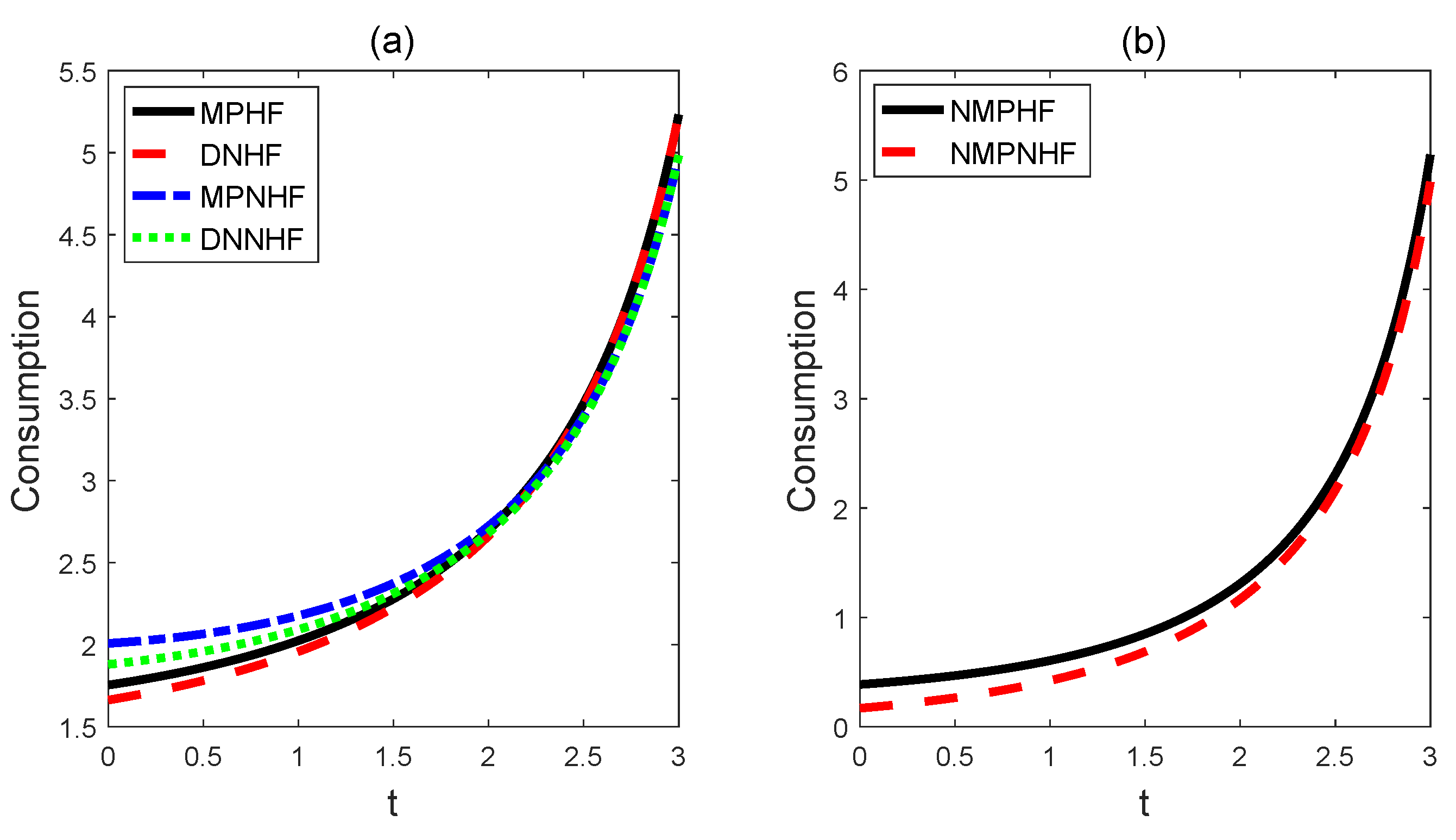
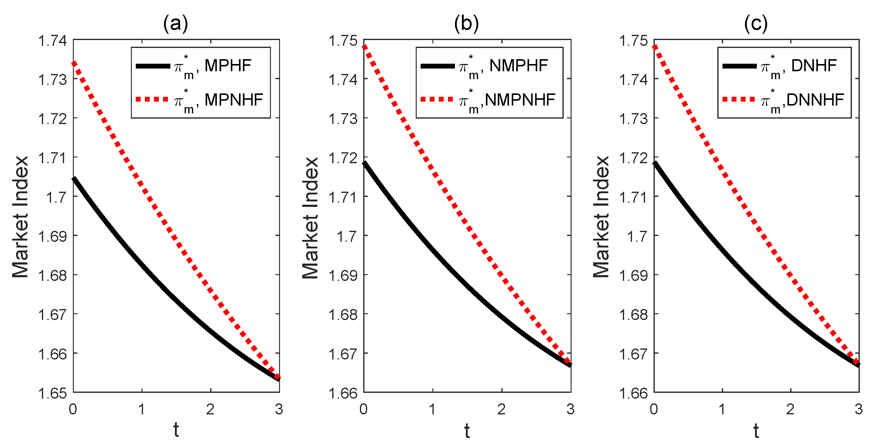
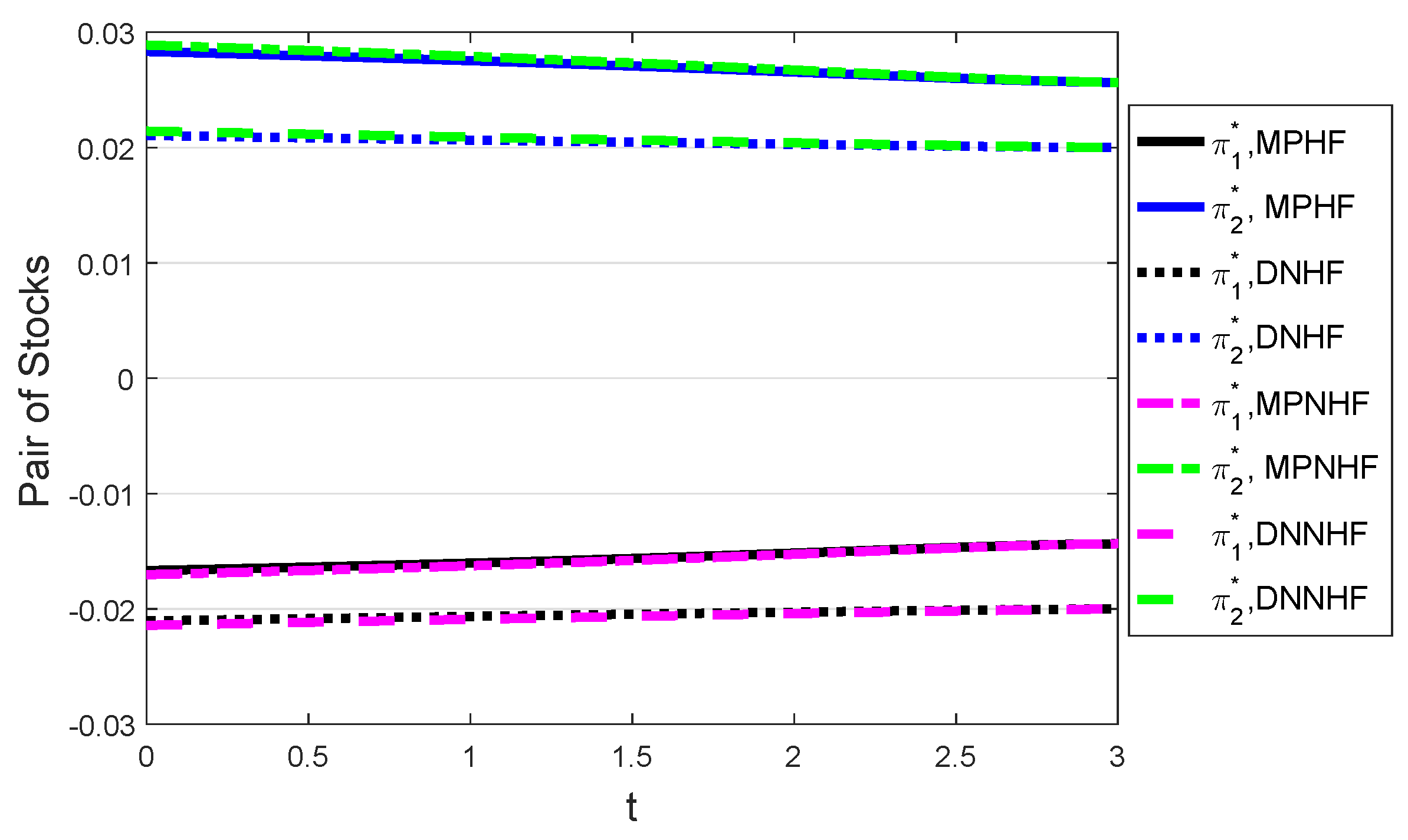
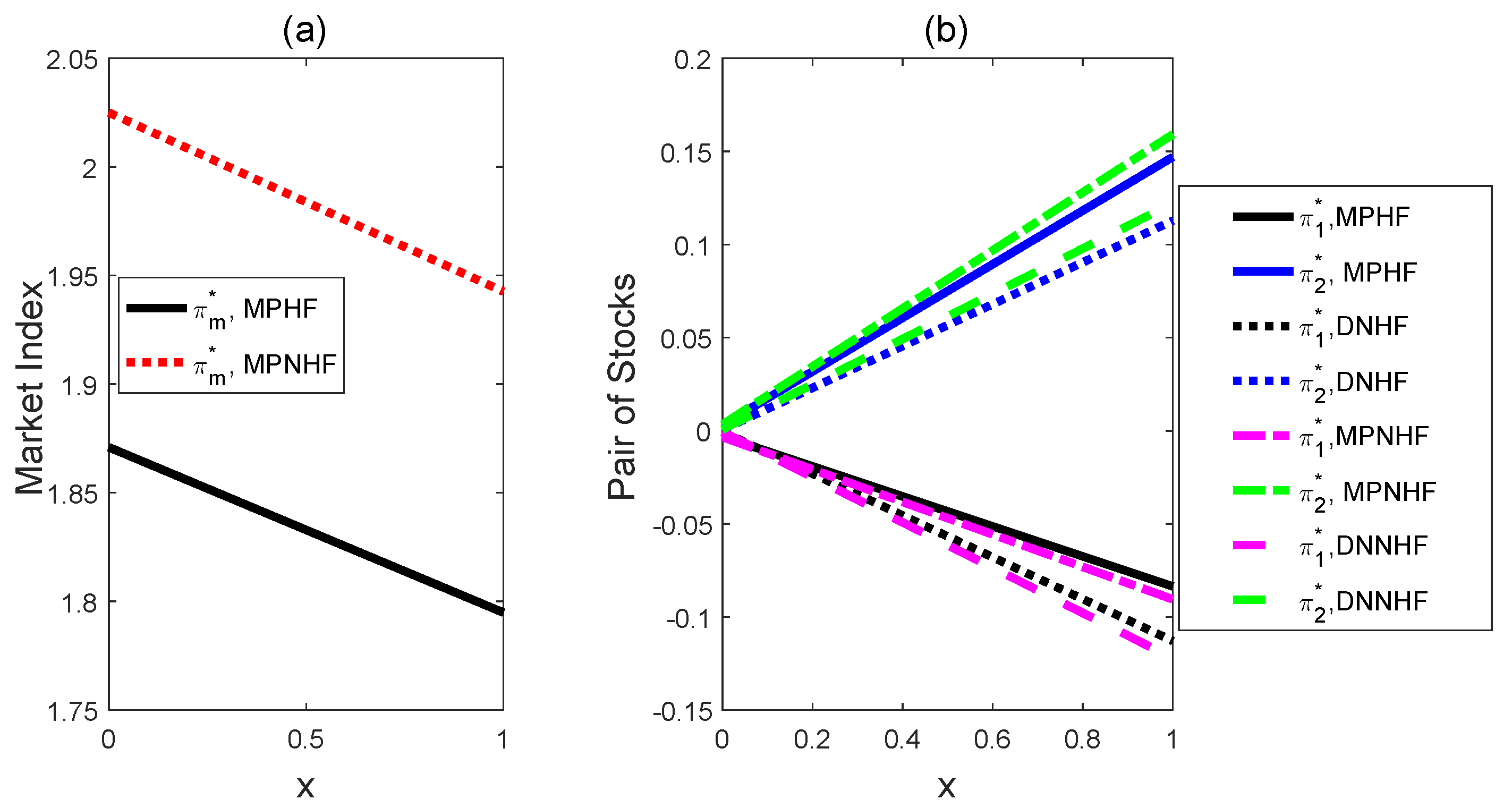
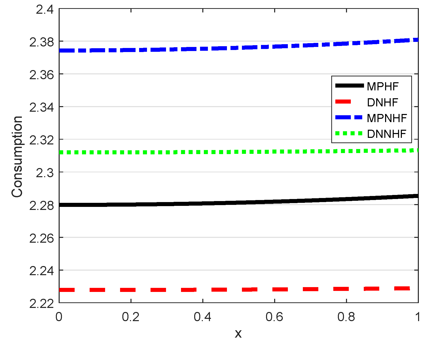
4.1. The Effects on Consumption and Investment Strategies

In the beginning, the following abbreviation terms are defined:

MPHF: The model involving mispricing and habit formation;

DNHF: The model involving the delta-neutral strategy and habit formation;

MPNHF: The model involving mispricing and no habit formation;

DNNHF: The model involving the delta-neutral strategy and no habit formation;

NMPHF: The model without mispricing but involving habit formation;

NMPNHF: The model without mispricing or habit formation.

In the figures of this paper, the consumption and portfolio weights of the wealth invested in the money account, bond stock, and index correspond to their expectations, respectively. Figure 1 graphs consumption as a function of time t. For a smaller t value (corresponding to a longer time horizon), when considering mispricing or the delta-neutral strategy (see Figure 1a), habit formation damps consumption. However, Figure 1b shows that habit formation increases consumption when ignoring mispricing, and taking the delta-neutral strategy diminishes consumption. For a larger t (corresponding to a shorter time horizon), consumption increases with time t, and the effects of habit formation and mispricing on consumption gradually disappear.

Figure 2a–c and Figure 3a,b show the portfolio weights of wealth invested in the market index, which decrease with time. Figure 2 shows that habit formation decreases the portfolio weights of wealth invested in the market index, while Figure 3 discloses that ignoring mispricing or adopting the delta-neutral strategy will increase it. Meanwhile, Figure 3 also shows that there is almost no difference between ignoring mispricing and adopting the delta-neutral strategy when investing in the market index.

Figure 4 illustrates the portfolio weights of wealth invested in the pair of mispriced stocks. (i) We find that, in the long run, the effects of habit formation on the stock investment are not obvious; however, for a larger pricing error x (see Figure 5b), habit formation has a significant impact on the pair of stocks. (ii) In our example, $X\left(t\right)=0.2,l_1=0.2,l_2=0.4$, which implies that the price of asset 1 is overestimated and asset 2 is underestimated. Therefore, in Figure 4, the agent shorts selling asset 1 and buys asset 2. Meanwhile, $l_2>l_1$ means that asset 2 has a stronger mispricing correction ability. Thus, we observe that the proportion of wealth spent on asset 2 is higher than that spent on asset 1. (iii) As t increases, i.e., the time horizon shortens, and the portfolio weights of wealth invested in the pair of mispriced stocks decrease. (iv) For the delta-neutral strategy, conclusions (i) and (iii) are also valid.

Figure 6 displays consumption as a function of the pricing error x. We reach get the following conclusion: habit formation limits consumption. When considering mispricing, consumption increases over the pricing error, while consumption has little change with pricing error when adopting the delta-neutral strategy.

We illustrate the proportions of wealth invested in the market index and a pair of stocks as functions of the pricing error in Figure 5. Figure 5a shows that the proportion of wealth invested in the market index decreases with the pricing error and is limited by habit formation. From Figure 5b, we can obtain the following results. On the one hand, as mentioned above, for a larger pricing error x, habit formation affects the proportions of wealth invested in the pair of stocks. On the other hand, as the pricing error increases, the proportion of short-selling asset 1 and buying asset 2 also increases. The reason is that increasing pricing errors will expand the statistical arbitrage opportunities between these two mispricing risky assets. This is also the reason why the proportion of wealth invested in the market index decreases.

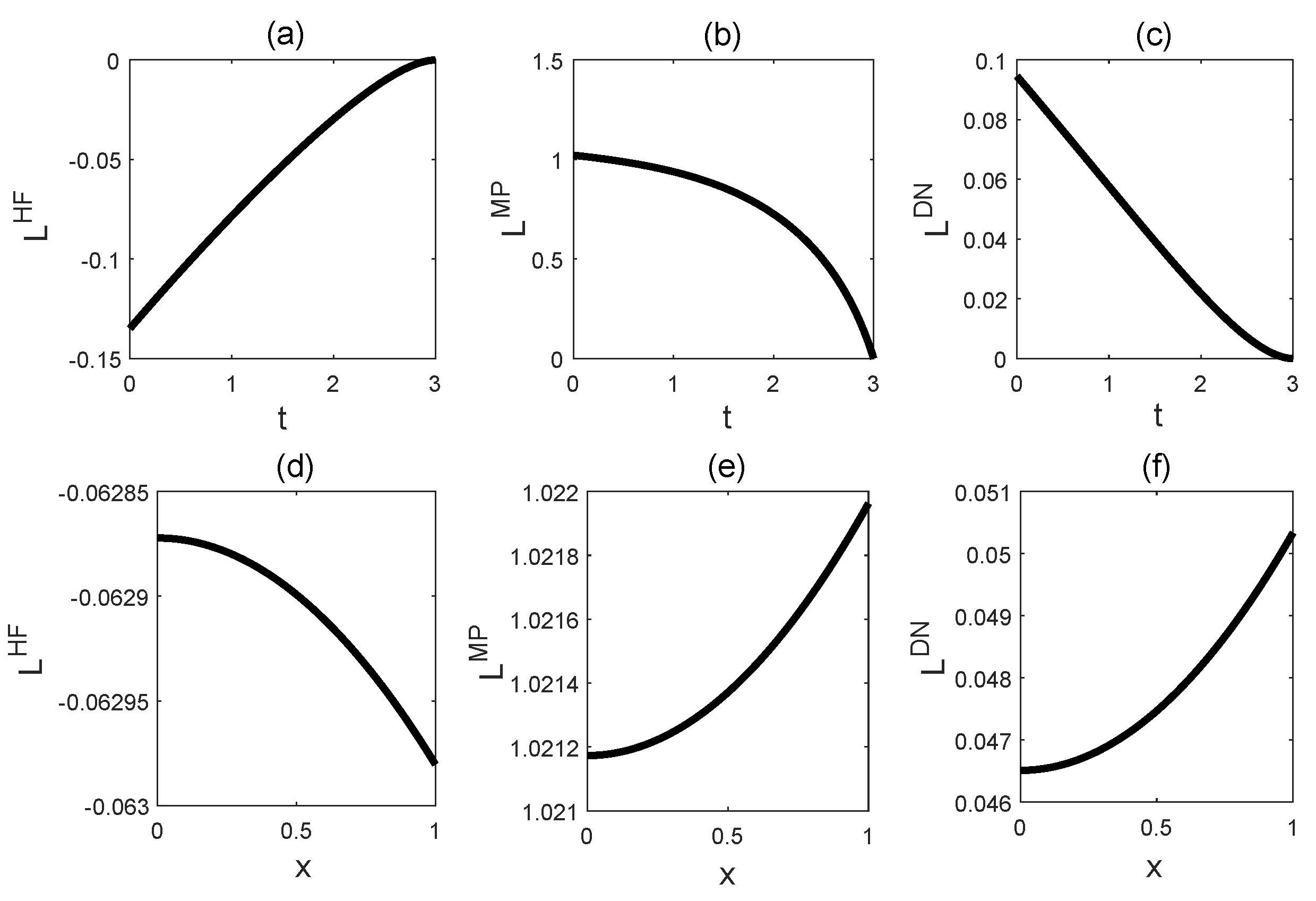
4.2. Wealth-Equivalent Utility Loss

Following Ref. [19], we define the wealth-equivalent utility loss (denoted by $L^{HF}$, $L^{MP}$ and $L^{DN}$) under three cases, including ignoring habit formation, ignoring mispricing, and adopting the delta-neutral arbitrage strategy. We have the following:

$$\begin{array}{c}\hfill L^{HF}=\left(1-{\left({\displaystyle \frac{\breve{f}(t,x)}{f(t,x)}}\right)}^{{\displaystyle \frac{\gamma }{1-\gamma }}}\right){\displaystyle \frac{w+A\left(t\right)y}{w}}-D\left(t\right){\displaystyle \frac{h}{w}},\end{array}$$

(52)

$$\begin{array}{c}\hfill L^{MP}=\left(1-{\left({\displaystyle \frac{\overline{f}\left(t\right)}{f(t,x)}}\right)}^{{\displaystyle \frac{\gamma }{1-\gamma }}}\right){\displaystyle \frac{w+A\left(t\right)y-D\left(t\right)h}{w}},\end{array}$$

(53)

$$\begin{array}{c}\hfill L^{DN}=\left(1-{\left({\displaystyle \frac{\tilde{f}(t,x)}{f(t,x)}}\right)}^{{\displaystyle \frac{\gamma }{1-\gamma }}}\right){\displaystyle \frac{w+A\left(t\right)y-D\left(t\right)h}{w}}.\end{array}$$

(54)

Figure 7 illustrates these wealth-equivalent utility losses. Based on Figure 7a,d, we observe that $L^{HF}<0$ for all time t or pricing error x, which implies that when one ignores habit formation, the utility loss does not decrease but instead increases. As mentioned above, when considering mispricing, habit formation damps consumption, leading to the agent’s utility (from consumption) decreasing. Thus, if one ignores habit formation, the utility will increase. Figure 7b,c,e,f show that ignoring mispricing or adopting the delta-neutral arbitrage strategy will lead to utility loss. The utility loss decreases with time t but increases as the pricing error increases.

5. Conclusions and Future Work

In this work, we formulate an investment and consumption model. The agent can invest the wealth in one risk-free asset, a market index and a pair of stocks with mispricing, in the financial market, and meanwhile consumes his/her income. The agent with habit formation can optimize strategies by investing mispricing assets. The optimization problem is to find the optimal consumption and investment strategies to maximize the expected utility from consumption and terminal wealth. Specifically, the utility from consumption originated from the difference between the consumption and habit level, i.e., from the part of the consumption that exceeds the habit level. Theoretically, a verification theorem for the solution of the optimization problem is provided, and we obtain the optimal value function and optimal strategies for the agents who overlook mispricing and those who take the delta-neutral arbitrage strategy for granted. In the numerical analysis, we discuss the impact of habit formation and mispricing on the optimal strategies. Specifically, this paper considers six cases of the model; that is, the case involving mispricing and habit formation, the case involving the delta-neutral strategy and habit formation, the case involving mispricing and no habit formation, the case involving the delta-neutral strategy and no habit formation, the case without mispricing but involving habit formation, and the case without mispricing or habit formation. The results indicate that the existence of mispricing and the consumption habits of agents can both affect their financial behaviors. This reminds us that when studying issues involving consumption and investment, we should acknowledge the existence of mispricing and consider the consumption habits of agents. Finally, we define and analyze the wealth-equivalent utility loss under three cases, including ignoring habit formation, ignoring mispricing, and adopting the delta-neutral arbitrage strategy.

There are some possible extensions of our model. Firstly, to simplify the model and obtain an analytical solution to the optimization problem, and to highlight the roles of mispricing and consumption habits, we assume that the agent’s income is non-random. In future work, we may consider the heterogeneity risk of income and present its effect on the optimal strategies. Secondly, we may consider an ambiguity-averse agent and investigate his/her specific preference for model ambiguity robustness, or we may consider preference with the time-varying coefficient of risk aversion, similar to Lichtenstern et al., (2021) [5]. Thirdly, our theoretical model suggests that mispricing and consumption habits impact financial behaviors in theory. Subsequently, we aim to apply this model to real-world scenarios and seek empirical validation in future work.

References

1. Merton, R.C. Lifetime portfolio selection under uncertainty: The continuous-time case. Rev. Econ. Stat. 1969, 51, 247–257. [Google Scholar] [CrossRef]
2. Bellalah, M.; Zhang, D.; Zhang, P. An optimal portfolio and consumption problem with a benchmark and partial information. Math. Financ. Econ. 2023, 17, 127–152. [Google Scholar] [CrossRef]
3. Cocco, J.F.; Gomes, F.J.; Maenhout, P.J. Consumption and portfolio choice over the life cycle. Rev. Financ. Stud. 2005, 18, 491–533. [Google Scholar] [CrossRef]
4. Bilsen, S.V.; Laeven, R.J. Dynamic consumption and portfolio choice under prospect theory. Insur. Math. Econ. 2020, 91, 224–237. [Google Scholar] [CrossRef]
5. Lichtenstern, A.; Shevchenko, P.V.; Zagst, R. Optimal life-cycle consumption and investment decisions under age-dependent risk preferences. Math. Financ. Econ. 2021, 15, 275–313. [Google Scholar] [CrossRef]
6. Gu, A.; Viens, F.G.; Bo, Y. Optimal reinsurance and investment strategies for insurers with mispricing and model ambiguity. Insur. Math. Econ. 2017, 72, 235–249. [Google Scholar] [CrossRef]
7. Liu, J.; Longstaff, F. 2004. Losing money on arbitrage: Optimal dynamic portfolio choice in markets with arbitrage opportunities. Rev. Financ. Stud. 2004, 17, 611–641. [Google Scholar] [CrossRef]
8. Liu, J.; Timmermann, A. Optimal convergence trade strategies. Rev. Financ. Stud. 2013, 26, 1048–1086. [Google Scholar] [CrossRef]
9. Yi, B.; Viens, F.; Law, B.; Li, Z. Dnynamic portfolio selection with mispricing and model ambiguity. Ann. Financ. 2015, 11, 37–75. [Google Scholar] [CrossRef]
10. Gu, A.; Viens, F.G.; Yao, H. Optimal robust reinsurance-investment strategies for insurers with mean reversion and mispricing. Insur. Math. Econ. 2018, 80, 93–109. [Google Scholar] [CrossRef]
11. Constantinides, G.M. Habit formation: A resolution of the equity premium puzzle. J. Political Econ. 1990, 98, 519–543. [Google Scholar] [CrossRef]
12. Browning, M.; Collado, D. Habits and heterogeneity in demands: A panel data analysis. J. Appl. Econom. 2007, 22, 625–640. [Google Scholar] [CrossRef]
13. Munk, C. Portfolio and consumption choice with stochastic investment opportunities and habit formation in preferences. J. Econ. Dyn. Control 2008, 32, 3560–3589. [Google Scholar] [CrossRef]
14. Li, W.; Tan, K.S.; Wei, P. Demand for non-life insurance under habit formation. Insur. Math. Econ. 2020, 101, 38–54. [Google Scholar] [CrossRef]
15. Shi, A.; Li, X.; Li, Z. Optimal portfolio selection with life insurance under subjective survival belief and habit formation. J. Ind. Manag. Optim. 2023, 19, 2464–2484. [Google Scholar] [CrossRef]
16. Detemple, J.B.; Zapatero, F. Asset prices in an exchange economy with habit formation. Econometrica 1991, 59, 1633–1657. [Google Scholar] [CrossRef]
17. Kraft, H.; Munk, C.; Wagner, S. Housing habits and their implications for life-cycle consumption and investment. Rev. Financ. 2018, 22, 1737–1762. [Google Scholar] [CrossRef]
18. Kraft, H.; Munk, C. Optimal housing, consumption, and investment decisions over the life cycle. Manag. Sci. 2011, 57, 1025–1041. [Google Scholar] [CrossRef]
19. Branger, N.; Larsen, L.S.; Munk, C. Robust portfolio choice with ambiguity and learning about return predictability. J. Bank. Financ. 2013, 37, 1397–1411. [Google Scholar] [CrossRef]
Figure 1. Consumption as a function of time t.
Mathematics 12 02248 g001
Figure 2. Proportion of wealth invested in the market index as a function of time t.
Mathematics 12 02248 g002
Figure 3. Proportion of wealth invested in the market index as a function of time t.
Mathematics 12 02248 g003
Figure 4. Proportion of wealth invested in the pair of mispriced stocks as a function of time t.
Mathematics 12 02248 g004
Figure 5. Proportions of wealth invested in risky assets as functions of pricing error x.
Mathematics 12 02248 g005
Figure 6. Consumption as a function of pricing error x.
Mathematics 12 02248 g006
Figure 7. The wealth-equivalent utility loss as a function of time and price error, respectively.
Mathematics 12 02248 g007