A Comprehensive Analytical Framework under Practical Constraints for a Cooperative NOMA System Empowered by SWIPT IoT

Abstract

Over the past decade, there has been notable attention directed towards spectrum and energy efficiency in conjunction with simultaneous wireless information and power transfer (SWIPT), aimed at extending the operational lifespan of energy-constrained wireless devices within cooperative non-orthogonal multiple access (C-NOMA) systems. This article delves into a system model comprising a transmitter, a relay, and two users, where the time-switching receiver (TSR) protocol is employed for energy harvesting at the relay. The objective of this study is to evaluate the performance of the system in terms of outage probability (OP), and system throughput (ST), and to determine the optimal time-switching (TS) factor. Our analysis encompasses the evaluation of OP, ST, and the determination of the optimal TS factor. Numerical simulation results reveal that the Nakagami-m fading channel exhibits the lowest outage probability, and that system throughput escalates with the signal-to-noise ratio (SNR) augmentation. These findings underscore the potential of the Nakagami-m fading channel to enhance energy efficiency in C-NOMA systems and suggest promising directions for future research.

1. Introduction

1.1. Information Background

NOMA represents a multiple access technique that integrates multiplexing and multi-user detection methods, enabling multiple users to share a single channel efficiently. In contrast to Frequency Division Multiple Access (FDMA) and Orthogonal Frequency Division Multiple Access (OFDM), which fall under the category of Orthogonal Multiple Access (OMA) techniques, NOMA presents a more effective means of leveraging the radio spectrum, exemplified by Orthogonal Frequency Division Multiple Access (OFDMA). NOMA facilitates more efficient resource utilization by allocating distinct portions of resources such as frequency, power, or codes to individual users. Moreover, it enables the provision of asymmetric data rates and diverse Quality of Service (QoS) standards, thus enhancing flexibility in service offerings [1,2]. The Time-Splitting Relaying (TSR) protocol has demonstrated notable efficacy in enhancing the performance of NOMA-Simultaneous Wireless Information and Power Transfer (SWIPT) systems, evident in improvements in both energy efficiency and data rate. Consequently, TSR stands as a valuable asset for researchers and engineers engaged in the development of C-NOMA-SWIPT systems [3]. In NOMA systems, the Decode-and-Forward (DF) approach serves as a cooperative relaying mechanism for SWIPT. Within NOMA setups, multiple users share the same frequency band, receiving identical signals from a singular base station (B). In SWIPT configurations, user equipment derives power from received wireless signals. Employing multiple relay nodes in the cooperative relaying process enhances communication link reliability and coverage area. In DF relaying, the relay node decodes the received signal, re-encodes it, and subsequently transmits it to the destination node. This method presents significant advantages in energy efficiency and communication performance over conventional single-hop communication systems. The fundamentals of DF relaying for SWIPT in NOMA systems and its advantages over other relaying strategies will be covered in this section [4,5,6]. NOMA has recently emerged as a promising candidate for future wireless networks due to its capacity for significant improvements in spectral and energy efficiency, as well as fairness [7,8]. Power domain NOMA employs techniques such as superimposed coding (SC) [9] and successive interference cancellation (SIC) [10,11] to combine transmission signals at the transmitter and decode reception signals at the receivers [12]. Consequently, it enables the source to serve multiple users using the same frequency/time resources [5]. Furthermore, in NOMA network systems, users are allocated different power levels to ensure fairness. This approach implies that users closer to the source receive less power compared to those farther away [13]. In C-NOMA scenarios [14], a user located at a distance with weaker channel conditions may require assistance from another user to relay the signal from the source to itself. This signal-forwarding process can occur in systems with or without obstacles. The inclusion of a relay user in C-NOMA facilitates the uninterrupted propagation of information to the intended destination. However, in obstacle-free systems, referred to as C-NOMA with direct link [15,16,17], the involvement of a cooperative user ensures the integrity and reliability of the transmitted signal for the distant user, even though the signal from the source can reach this user directly. At user relay, amplify-and-decode (AF) [18], DF [19,20] schemes are utilized to harvest energy and forward information to the destination. As SWIPT [21] is exploited at the user relay in C-NOMA, it can combine with power-splitting relaying (PSR) and TSR [22] protocols for simultaneous EH and information decoding. The energy harvested at R is to maintain its lifetime due to battery limitations. In [23], a full-duplex (FD) cooperative NOMA model with one BS and two users was studied. Both direct link and no direct link between the BS and far user were considered. In [17], a C-NOMA with and without a direct link was investigated. The closed-form outage probability expression was derived for both no direct link and direct link. The OP for FD NOMA is better than that for half-duplex (HD) NOMA. Besides, throughput, ergodic rate and energy efficiency were evaluated for FD and HD NOMA.

1.2. Related Works and Motivation

C-NOMA can operate in both HD and FD modes [24,25]. Due to the simultaneous reception and transmission of signals in the same time slot and frequency band, FD mode can improve the spectral efficiency of the NOMA system by up to two times compared to HD mode [14,15,16]. Therefore, FD relay technology has been shown as a promising scheme for 5G-based wireless networks. In [25], an FD multi-antenna relay-assisted C-NOMA network was examined. The system comprised one BS, a cognitive near user, and a cognitive far user. An optimization problem regarding user rate was addressed, revealing that the impact of residual self-interference at the FD relay and inter-user interference in the near-user scenario could be significantly mitigated. Both analytical and simulation-based assessments were conducted to determine the outage performance in [23]. The study in [23] also demonstrated that FD NOMA exhibits a lower OP than HD NOMA in the low Signal-to-Noise Ratio (SNR) region. Additionally, the system throughput for Delay-Limited Transmission (DLT) mode in FD NOMA surpassed that of HD NOMA. Furthermore, in [15], the outage performance of the proposed FD C-NOMA scheme, specifically an FD device-to-device (D2D) aided C-NOMA scheme, outperformed that of conventional NOMA and OMA. The expressions for outage probability were also derived in the same work. In [26], the authors investigated the confidentiality performance of cooperative NOMA systems integrating EH and FD relaying employing power splitting protocol over experience-independent, non-selective block Rayleigh fading. Their emphasis was on deriving closed-form expressions for EH-FD-NOMA, encompassing the lower bound on ergodic secrecy rates and the approximated secrecy OPs for the two users. In [27], the authors investigated a cooperative communication scheme that combines C-NOMA, FD relaying, and EH techniques through the utilization of a TS protocol over independent Rayleigh fading channels. They derived closed-form expressions to evaluate the performance of the proposed EH-FD-NOMA system, including OPs and ergodic rates. In [28], the authors introduced a Cooperative Spectrum-Sharing Transmission (CSST) scheme employing the DF relaying strategy. Their study incorporated realistic considerations such as FD-based loop self-interference, NOMA-based imperfect successive interference cancellation, and transceiver hardware impairments in Internet of Things (IoT) devices. Utilizing Nakagami-m fading environments, a comprehensive performance analysis was conducted by deriving expressions for the OP for both primary and secondary networks within the FD-based CSST scheme under both TS and PS protocols. NOMA-SWIPT takes center stage as an indispensable requisite in the landscape of IoT networks. In a time marked by the explosive proliferation of IoT devices, where the optimization of both energy and spectral efficiency reigns supreme, NOMA-SWIPT emerges as a revolutionary remedy. By facilitating the concurrent sharing of scarce spectrum resources among multiple IoT devices, NOMA not only fine-tunes spectral utilization but also furnishes the critical capability of wireless power transfer. This dual-faceted functionality transcends mere convenience; it becomes imperative, particularly in scenarios where IoT devices are deployed in remote or inaccessible locales, challenging the provision of continuous power supply. Consequently, NOMA-SWIPT assumes the pivotal role of empowering IoT networks to unlock their full potential, cultivating sustainable, ever-connected ecosystems that catalyze innovation and drive efficiency across a spectrum of industries [29,30,31,32]. In addition,

Table 1. Comparison between the novelty of our work and previous papers (X: Not Discussed; ✓: Discussed.

	Our Scheme	[33]	[34]	[4]	[5]	[6]	[35]	[36]	[37]
NOMA	✓	✓	✓	✓	✓	✓	X	X	✓
Multiple Relay	X	X	X	X	X	X	X	✓	X
Energy harvesting	✓	✓	✓	✓	✓	✓	✓	✓	✓
Generalized channels	✓	X	X	X	X	X	X	X	X
Full-Duplex	X	✓	✓	X	X	X	X	X	X
Power beacon	✓	X	X	X	X	X	X	✓	✓
AF	X	X	X	X	X	X	✓	X	X
DF	✓	✓	✓	✓	✓	✓	X	✓	✓
Outage Probability	✓	✓	✓	✓	✓	✓	X	✓	✓
Throughput	✓	✓	✓	✓	✓	✓	X	✓	✓
Optimization	✓	X	✓	X	X	X	X	X	✓

summarizes the related works.

1.3. Contributions

Within the domain of SWIPT IoT systems employing C-NOMA techniques, this paper presents a series of substantial contributions:

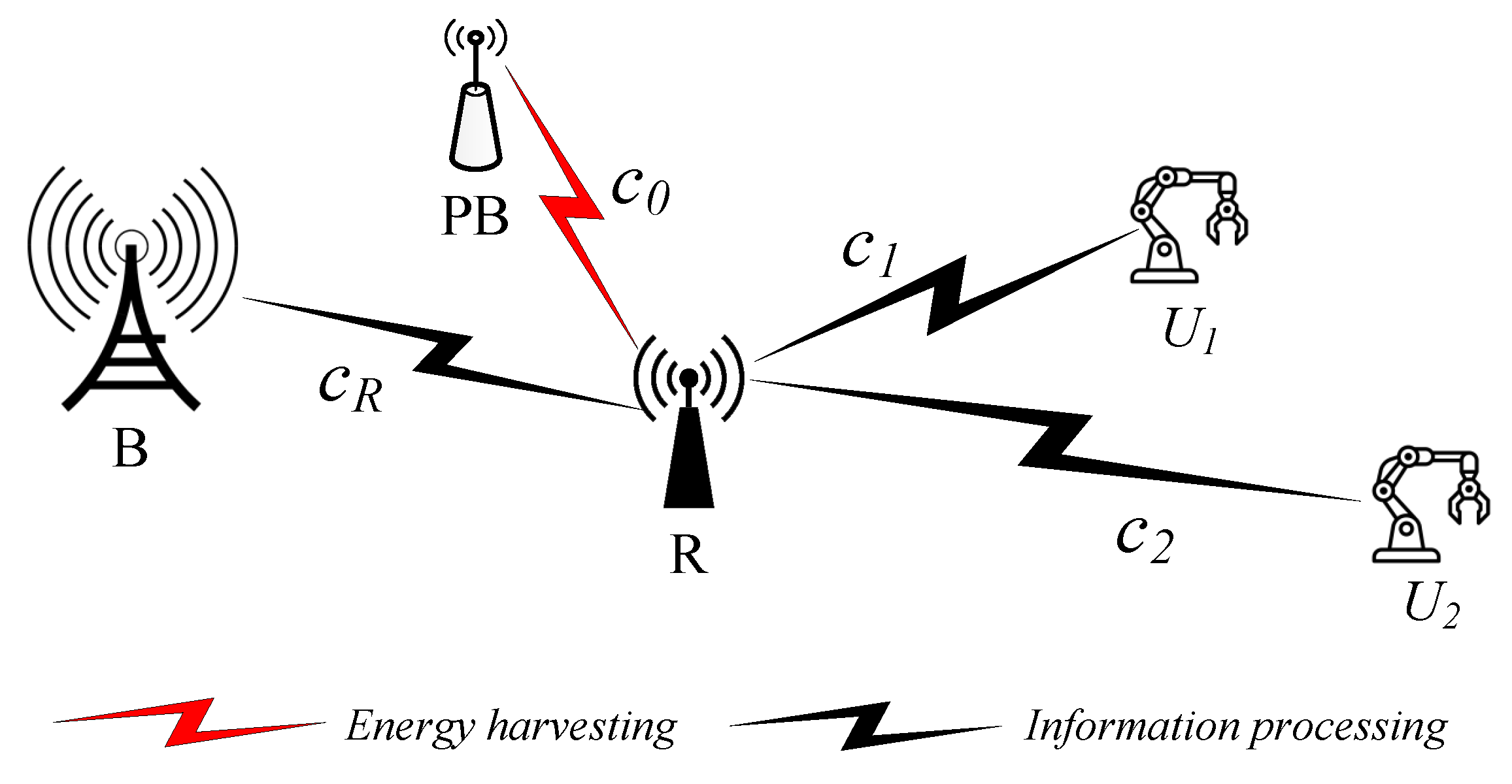
• An innovative C-NOMA scheme custom-tailored for SWIPT-enabled IoT systems takes center stage. This scheme orchestrates power allocation for two users through a pivotal relay node (R) in the DF of signals from the B. It is essential to emphasize that R also performs the critical task of EH from the power beacon (PB). This holistic integration of power management, signal manipulation, and EH within a unified relay node represents a groundbreaking strategy, aimed at optimizing overall system efficiency. The scheme utilizes a TS receiver architecture, enabling R to simultaneously perform both EH and Information Processing (IP) tasks.
• EH Protocol Advancement: The paper introduces an advanced EH protocol with an HD-based TSR mechanism meticulously designed for SWIPT-based C-NOMA systems. This EH protocol assumes a pivotal role in the harnessing of energy from received signals, thereby bolstering the sustainability and autonomy of IoT devices interconnected within the network.
• In an effort to provide a comprehensive understanding of system performance, the paper derives precise closed-form expressions for critical metrics, including but not limited to OP and System Throughput (ST). These analytical expressions serve as essential tools for rigorously evaluating the proposed C-NOMA and EH schemes. Researchers and practitioners can use these insights to make informed decisions and assess the effectiveness of these systems in practical IoT deployments.

1.4. Organization and Notations

Organization: The paper is organized as follows: Section 2 introduces the system model of the relay-assisted C-NOMA along with its assumptions. Section 3 outlines the energy harvesting process at the relay node based on time-switching relaying. Section 4 delves into the analysis of performance evaluation. Section 5 focuses on determining the optimal time-switching factor to minimize the outage probability of users. Section 6 elaborates on the simulation results. Finally, Section 7 offers conclusions and summarizes the key findings of this study. The abbreviations and acronyms are presented in

Table 2. Abbreviations and Acronyms.

Acronym	Definition
6G	Six-generation
AF	Amplify and decode
AWGN	Additive white gaussian noise
CDF	Cumulative distribution function
C-NOMA	Cooperative non-orthogonal multiple access
CSST	Cooperative spectrum-sharing transmission
D2D	Device to device
DF	Decode and forward
DLT	Delay-limited transmission
EH	Energy harvesting
FD	Full-duplex
HD	Half-duplex
IoT	Internet of things
IP	Information processing
ipSIC	Imperfect SIC
LEH	Linear energy harvesting
NLEH	Nonlinear energy harvesting
OFDM	Orthogonal frequency division multiple access
OFDMA	Orthogonal frequency division multiple access
OMA	Orthogonal multiple access
OP	Outage probability
PDF	Probability density function
pSIC	Perfect SIC
QoS	Quality of service
RMS	Root-mean-square
RVs	Random variables
SC	Superimposed coding
SIC	Successive interference cancellation
ST	System throughput
SINR	signal-to-plus-noise ratio
SNR	signal-to-noise ratio
SWIPT	Simultaneous wireless information and power transfer
TSR	Time-switching receiver

.

Notations: The notation $\mathbb{E}\left[.\right]$ stands for the operation of calculating expectation. $f_X(.)$ and $F_X(.)$ denote the probability density function (PDF) and the cumulative distribution function (CDF) of a random variable X, respectively.

2. System Model

The system model under investigation is illustrated in Figure 1. In this system, the signal is transmitted from source B to two users, namely $U_1$ and $U_2$, via relay node R. R operates as a DF relay to forward the information from B to $U_1$ and $U_2$. The relays are power-limited devices and rely on the support of a PB. We denote the parameters of the system model as follows: $c_r$ represents the channel coefficients from the source PB to R, while $c_0$, $c_1$, and $c_2$ represent the channel coefficients from the source B to R and from R to $U_1$ and $U_2$, respectively.

In this system model, we assume that there are no additional power sources embedded in the relay node to provide energy. Hence, in the initial phase, the relay node harvests energy from neighboring nodes, i.e., source B and the destinations $U_1$ and $U_2$ shown in the figure, to facilitate the forwarding of information. Specifically, this harvested energy can be stored in the batteries so that it can then be reused to forward the information from B to $U_1$ and $U_2$. The channels have power gains ${\left|c_R\right|}^2$, ${\left|c_0\right|}^2$, ${\left|c_1\right|}^2$, ${\left|c_2\right|}^2$. The power gains are distributed according to exponential RVs with ${\mathsf{\Omega }}_i,i\in \left\{0,1,2\right\}$, respectively. It is assumed that all wireless links are non-selection blocks and independent Rayleigh fading and are impacted by AWGN with average power $N_0$.

3. The TSR-Based Energy Harvesting of the Relay Node

3.1. The Energy Harvesting at the Relay Node

The EH scheme involving time and power is depicted in Figure 2. Within $\varrho T$, the B transfers energy to R via a single antenna with consistent sending power (referred to as the energy-transfer phase). In this context, T and $\varrho \in \left[0,1\right]$, signify the coherence time block and the TS ratio, respectively. During the period referred to as the data transmission phase, which lasts for $\left(1-\varrho \right)T$, R transmits message information signals to two users in the second hop, while B simultaneously broadcasts the aggregated signals from the users to the R node in the first hop.

3.2. Phase: Energy Transfer

During this phase, the receiver uses its resources to collect radio frequency energy from the power beacon during a time slot labeled as $\varrho T$. Here, $\varrho$ represents the time switching ratio, and T denotes the duration of the block time period. The energy harvested through this process can be precisely described as follows:

$$E_r=\eta \varrho T{P}_B{\left|c_0\right|}^2.$$

(1)

In this case, $\eta \in \left(0,1\right)$ indicates the energy conversion efficiency of the B, while $P_B$ stands for the transmit power of the B. Let us denote ${\left|c_0\right|}^2$ as the channel coefficient from B to R. Following the nonlinear energy-harvesting approach outlined in [38], the transmit power of R acquired over the duration of $\left(1-\varrho \right)T/\phantom{\left(1-\varrho \right)T2}2$ can be expressed as:

$$\begin{array}{cc}\hfill P_r=& {\displaystyle \frac{2E_r}{\left(1-\varrho \right)T}}\hfill \\ \hfill =& \left\{\begin{array}{cc}{\displaystyle \frac{2\eta \varrho P_B{\left|c_0\right|}^2}{\left(1-\varrho \right)}}& , \varrho P_B{\left|c_0\right|}^2\le \iota \\ {\displaystyle \frac{2\eta \varrho \iota }{\left(1-\varrho \right)}}& , \varrho P_B{\left|c_0\right|}^2>\iota \end{array}\right.\hfill \end{array}$$

(2)

where $\iota$ is the power saturation threshold.

3.3. Phase: Data Transmission

3.3.1. Stage. 1: Communication

During the initial time slot, B transmits the overlaid mixture, $\sqrt{{\alpha }_1{P}_B}{s}_1+\sqrt{{\alpha }_2{P}_B}{s}_2$, where $s_i$ and ${\alpha }_i$ represent the signal and power allocation coefficient of user i, respectively. Notably, ${\alpha }_1+{\alpha }_2=1$, and it is assumed that ${\alpha }_1<{\alpha }_2$. The baseband received signal at R can thus be expressed as follows:

$$y_r=c_{r}x+n_r=c_r\left(\sqrt{{\alpha }_1{P}_B}{s}_1+\sqrt{{\alpha }_2{P}_B}{s}_2\right)+n_r,$$

(3)

where $n_r\sim \mathcal{C}\mathcal{N}\left(0,N_0\right)$ is the AWGN component at R. At first, R decodes the $U_2$’s message using SIC and based on the NOMA principle it decodes its own message. To decode the messages $s_2$ and $s_1$ at R, the corresponding SINR and SNR can be expressed as follows:

$${\gamma }_r^{s_2}={\displaystyle \frac{{\alpha }_2{P}_B{\left|c_r\right|}^2}{{\alpha }_1{P}_B{\left|c_r\right|}^2+N_0}}={\displaystyle \frac{{\alpha }_2{\rho }_B{\overline{\gamma }}_r}{{\alpha }_1{\rho }_B{\overline{\gamma }}_r+1}},$$

(4)

and

$${\gamma }_r^{s_1}={\displaystyle \frac{{\alpha }_1{\rho }_B{\overline{\gamma }}_r}{\delta a_2{\rho }_B{\overline{\gamma }}_r+1}},$$

(5)

Here, ${\overline{\gamma }}_r\stackrel{\Delta }{=}{\left|c_r\right|}^2$, ${\rho }_B={\displaystyle \frac{P_B}{N_0}}$ depicts the SNR level at the transmitter side and the residual noise interference is represented by $\delta$. In real-world scenarios of NOMA systems, achieving pSIC might not always be possible. Therefore, if $\delta =0$, $U_1$ employs pSIC to decode the received signal. However, if $\delta$ ranges between $0<\delta \le 1$, $U_1$ resorts to ipSIC.

3.3.2. Stage. 2: Communication

During the second time slot, relays transmit this information to $U_1$ and $U_2$. Thus, the received signal at $U_i$, $i\in \left\{1,2\right\}$ can be expressed as follows:

$$y_{U_i}=c_i\left(\sqrt{{\alpha }_1{P}_r}{s}_1+\sqrt{{\alpha }_2{P}_r}{s}_2\right)+n_{U_i},$$

(6)

Here, $c_i$ represents the channel gain between the relay and $U_i$, and $n_{U_i}\sim \mathcal{C}\mathcal{N}\left(0,N_0\right)$ represents the AWGN noise at $U_i$. Following the SIC principle, $U_2$ decodes symbol $s_2$ while treating $s_1$ as noise. Based on Equation (6), SINR at $U_2$ is given by:

$${\gamma }_{U_2}^{s_2}={\displaystyle \frac{{\alpha }_2{P}_r{\left|c_2\right|}^2}{{\alpha }_1{P}_r{\left|c_2\right|}^2+N_0}}.$$

(7)

Replace Equation (2) with Equation (7) we have:

$${\gamma }_{U_2}^{s_2}=\left\{\begin{array}{cc}{\displaystyle \frac{{\alpha }_2\chi {\overline{\gamma }}_{0,2}}{{\alpha }_1\chi {\overline{\gamma }}_{0,2}+1}}& ,\varrho {\rho }_B{\left|c_0\right|}^2\le \iota \\ {\displaystyle \frac{{\alpha }_2\tilde{\chi }{\left|h_2\right|}^2}{{\alpha }_1\tilde{\chi }{\left|c_2\right|}^2+1}}& ,\varrho {\rho }_B{\left|c_0\right|}^2>\iota \end{array}\right.$$

(8)

where ${\overline{\gamma }}_{0,2}\stackrel{\Delta }{=}{\left|c_0\right|}^2{\left|c_2\right|}^2$ and $\chi ={\displaystyle \frac{2\eta \varrho {\rho }_B}{\left(1-\varrho \right)}}$. It is important to note that at $U_1$, both $s_1$ and $s_2$ are present simultaneously. Consequently, using the SIC method, $U_1$ needs to decode $s_1$. By considering the low-power signal $s_1$ as interference and utilizing SIC to eliminate it, $U_1$ can then extract the symbol $s_1$ by decoding the high-power symbol $s_2$. Consequently, the received SINR for $s_2$ at $U_1$ can be formulated as follows:

$${\gamma }_{U_1}^{s_2}={\displaystyle \frac{{\alpha }_2{P}_r{\left|c_1\right|}^2}{{\alpha }_1{P}_r{\left|c_1\right|}^2+N_0}}=\left\{\begin{array}{cc}{\displaystyle \frac{{\alpha }_2\chi {\overline{\gamma }}_{0,1}}{{\alpha }_1\chi {\overline{\gamma }}_{0,1}+1}}& ,\varrho {\rho }_B{\left|c_0\right|}^2\le \iota \\ {\displaystyle \frac{{\alpha }_2\tilde{\chi }{\left|c_1\right|}^2}{{\alpha }_1\tilde{\chi }{\left|c_1\right|}^2+1}}& ,\varrho {\rho }_B{\left|c_0\right|}^2>\iota \end{array}\right.$$

(9)

Here, ${\overline{\gamma }}_{0,1}\stackrel{\Delta }{=}{\left|c_0\right|}^2{\left|c_1\right|}^2$. Once canceled, the signal $s_2$ is only partially removed and transforms into interference. The SINRs of symbol $s_1$ at $U_1$ are given as follows:

$${\gamma }_{U_1}^{s_1}=\left\{\begin{array}{cc}{\displaystyle \frac{{\alpha }_1\chi {\overline{\gamma }}_{0,1}}{\delta {\alpha }_2\chi {\overline{\gamma }}_{0,1}+1}}& ,\varrho {\rho }_B{\left|c_0\right|}^2\le \iota \\ {\displaystyle \frac{{\alpha }_1\tilde{\chi }{\left|c_1\right|}^2}{\delta {\alpha }_2\tilde{\chi }{\left|c_1\right|}^2+1}}& ,\varrho {\rho }_B{\left|c_0\right|}^2>\iota \end{array}\right.$$

(10)

Similarly, at R, when $\delta =0$ and $0<\delta \le 1$, it corresponds to the cases of pSIC and ipSIC, respectively.

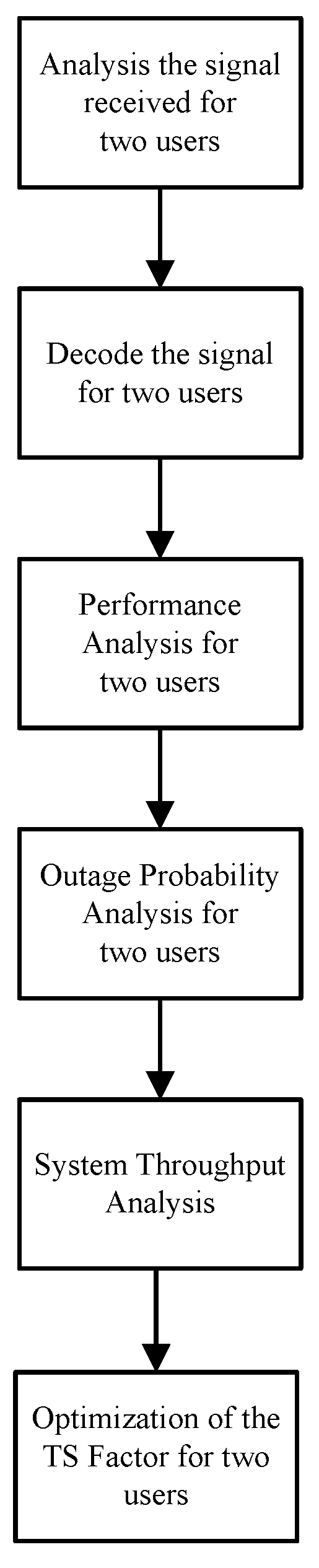
4. Performance Assessment

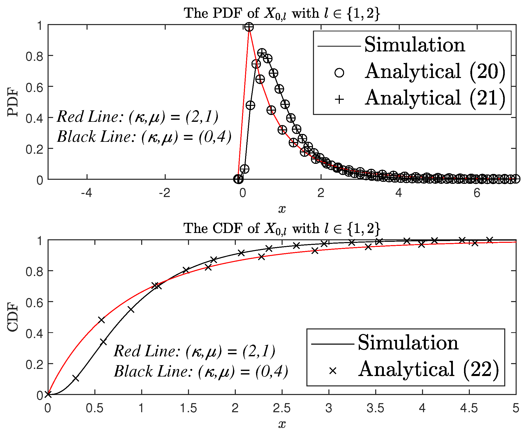
4.1. Channel Characteristics

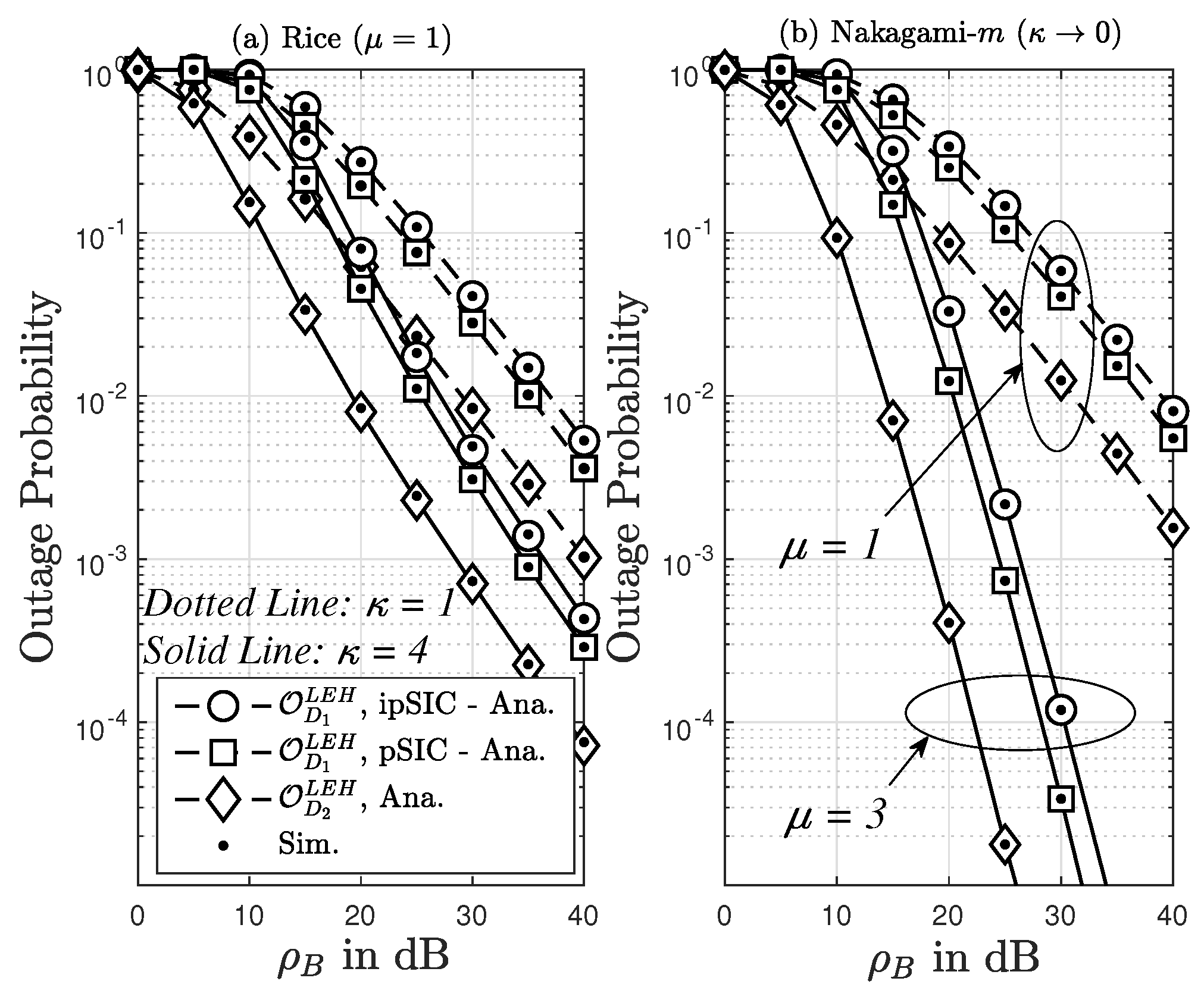
Let us examine two distinct random variables following the $\kappa -\mu$ distribution, each characterized by the PDF as shown in Equation (11).

$$\begin{array}{c}{f}_{T_e}\left(r\right)={\displaystyle \frac{2{\mu }_e{\left(1+{\kappa }_e\right)}^{\frac{{\mu }_e+1}{2}}{r}^{{\mu }_e}}{{\kappa }_e^{\frac{{\mu }_e-1}{2}}{e}^{{\mu }_e{\kappa }_e}{\widehat{r}}_e^{{\mu }_e+1}}}{e}^{-{\displaystyle \frac{{\mu }_e\left(1+{\kappa }_e\right)r^2}{{\widehat{r}}_e^2}}}{I}_{{\mu }_e-1}\left(2{\mu }_e\sqrt{{\kappa }_e\left(1+{\kappa }_e\right)}{\displaystyle \frac{r}{{\widehat{r}}_e}}\right),\hfill \end{array}$$

(11)

In the given context, where ‘e’ belongs to the set of real numbers, including 0, 1, and 2, ${\kappa }_e$, which is greater than 0, represents the ratio between the combined power of the primary components and that of the scattered waves. ${\mu }_e$, also greater than 0, is influenced by the quantity of multipath clusters. The function $I_v\left(s\right)$ refers to the modified Bessel function of the first kind and order ‘v’, while ${\widehat{r}}_e$ represents the root-mean-square (RMS) value of the received signal envelope, denoted as $T_e$. As described in reference [23], we have:

$$\begin{array}{c}{\widehat{r}}_e=\sqrt{\mathbb{E}\left\{T_e^2\right\}}={\displaystyle \frac{\sqrt{{\mu }_e\left(1+{\kappa }_e\right)}{\overline{r}}_e\Gamma \left({\mu }_e\right)}{{}_{1}F_1\left({\mu }_e+0.5;{\mu }_e;{\kappa }_e{\mu }_e\right)e^{-{\kappa }_e{\mu }_e}\Gamma \left({\mu }_e+0.5\right)}},\hfill \end{array}$$

(12)

$$\begin{array}{c}\mathbb{E}\left\{T_e^l\right\}={\displaystyle \frac{{}_{1}F_1\left({\mu }_e+0.5l;{\mu }_e;{\kappa }_e{\mu }_e\right)e^{-{\kappa }_e{\mu }_e}{\widehat{r}}_e^l\Gamma \left({\mu }_e+0.5l\right)}{{\left[{\mu }_e\left(1+{\kappa }_e\right)\right]}^{\frac{l}{2}}\Gamma \left({\mu }_e\right)}}.\hfill \end{array}$$

(13)

In this context, ${\overline{r}}_e=\mathbb{E}\left[T_i\right]$, where $\mathbb{E}\left[s\right]$ denotes the expectation operator, and ${\overline{r}}_e=\mathbb{E}\left[T_e^l\right]$ signifies the lth moment of $T_e$. Additionally, ${}_{1}F_1(s;y;z)$ refers to the confluent hypergeometric function, and $\Gamma (.)$ represents the Gamma function.

If we let ${\overline{\gamma }}_e$ denote the instantaneous SNR of $\kappa -\mu$ fading channel, we can derive the PDF of its instantaneous SNR ${\overline{\gamma }}_e$ from the envelope PDF provided in Equation (11) by employing a variable transformation $r=\sqrt{{\displaystyle \frac{x{\widehat{r}}_e^2}{{\mathsf{\Omega }}_e}}}$, which converts ${\overline{\gamma }}_e$ into a fading channel, as described in Equation (14).

$$\begin{array}{c}{f}_{{\overline{\gamma }}_e}\left(s\right)={\displaystyle \frac{{\mu }_e{\left(1+\kappa \right)}^{\frac{{\mu }_e+1}{2}}{s}^{\frac{{\mu }_e-1}{2}}}{{\kappa }_e^{\frac{{\mu }_e-1}{2}}{e}^{{\mu }_e{\kappa }_e}{\mathsf{\Omega }}_e^{\frac{{\mu }_e+1}{2}}}}{e}^{-{\displaystyle \frac{{\mu }_e\left(1+{\kappa }_e\right)x}{{\mathsf{\Omega }}_e}}}{I}_{{\mu }_e-1}\left(2{\mu }_e\sqrt{{\displaystyle \frac{{\kappa }_e\left(1+{\kappa }_e\right)}{{\mathsf{\Omega }}_e}}s}\right),\hfill \end{array}$$

(14)

where ${\mathsf{\Omega }}_e=\mathbb{E}\left[{\overline{\gamma }}_e\right]$. The modified Bessel function of the first kind from [39] (Eq. (9.6.16)), (14) is substituted as $I_v\left(u\right)={\sum }_{b=0}^{\infty }1/\phantom{1b!\Gamma \left(b+v+1\right)}b!\Gamma \left(b+v+1\right){\left(u/\phantom{u2}2\right)}^{2b+v}$ and defining ${\psi }_e={\mu }_e\left(1+{\kappa }_e\right)/\phantom{{\mu }_e\left(1+{\kappa }_e\right){\mathsf{\Omega }}_e}{\mathsf{\Omega }}_e$, (14) can be re-written as follows:

$$\begin{array}{c}{f}_{{\gamma }_e}\left(s\right)={\displaystyle \frac{1}{e^{{\mu }_e{\kappa }_e}}}{\displaystyle \sum _{b=0}^{\infty }}{\displaystyle \frac{{\left({\mu }_e{\kappa }_e\right)}^b{\psi }_e^{b+{\mu }_e}}{b!\Gamma \left(b+{\mu }_e\right)}}{x}^{b+{\mu }_e-1}{e}^{-{\psi }_{e}s}\hfill \\ \\ ={\displaystyle \frac{1}{e^{{\mu }_e{\kappa }_e}}}{\displaystyle \sum _{b=0}^{\infty }}{\displaystyle \frac{{\left({\mu }_e{\kappa }_e\right)}^b{\psi }_e^{b+{\mu }_e}}{b!\Gamma \left(b+{\mu }_e\right)}}\Gamma \left(b+{\mu }_e,{\psi }_e\right),\hfill \end{array}$$

(15)

where $\Gamma \left({\Xi }_e,{\Delta }_e\right)$ refer to the PDF of the gamma distribution as in Equation (16)

$$f_{Z_e}\left(z\right)={\displaystyle \frac{{\Delta }_e^{{\Xi }_e}}{\Gamma \left({\Xi }_e\right)}}{z}^{{\Xi }_e-1}{e}^{-z{\Delta }_e},$$

(16)

The form parameter is denoted by ${\Xi }_e$, while the rate parameter, represented by ${\Delta }_e$, serves as an inverse scale parameter.

Table 3. Simulation Parameters.

Parameters	Description
$R_i$	The target rate is set at $U_i$, where i belongs to the set $\left\{1,2\right\}$.
$s_i$	$U_i$’s information
${\epsilon }_i$	$U_i$’s threshold rate.
${\alpha }_i$	Power allocation coefficients at $U_i$.
$n_R$ & $n_{U_i}$	The AWGN term was succeeded by $\mathcal{C}\mathcal{N}(0,N_0)$.
$P_B$	Transmit power at BS.
$P_r$	Transmit power at R
T	The total time used for EH and IP.
$\varrho$	Time-switching factor.
$\eta$	The EH efficiency.
e	Subindex for defining the $e^{th}$RV. Here, $e\in \left\{R,0,1,2\right\}$
${\kappa }_e$	The ratio of the dispersed waves to the total power of the dominant components.
${\mu }_e$	An extension utilizing real values that are linked to the quantity of multipath clusters.
${\widehat{r}}_e$	The root-mean-square (RMS) value of the received signal envelope.
${\overline{r}}_e$	The average value of the received signal envelope.
${\gamma }_e$	The instantaneous signal-to-noise ratio (SNR).
${\mathsf{\Omega }}_e$	The average SNR.
${\Xi }_e$	The shaping parameter refers to a crucial aspect of a Nakagami-m RV.
${\Delta }_e$	The rate parameter (also known as the inverse scale parameter) represents an optimistic measure of a Gamma RV.

summarizes the notations employed in this document.

The CDF of ${\overline{\gamma }}_e$ is given by:

$$\begin{array}{cc}{F}_{{\overline{\gamma }}_e}\left(s\right)=1-{\mathcal{Q}}_{{\mu }_e}\left(\sqrt{2{\kappa }_e{\mu }_e},\sqrt{2{\psi }_{e}s}\right)& ,s>0,\end{array}$$

(17)

where ${\mathcal{Q}}_c\left(e,b\right)=e^{1-c}{\int }_b^{\infty }{s}^c{e}^{-\left(s^2+e^2\right)/\phantom{\left(s^2+e^2\right)2}2}{\mathcal{I}}_{c-1}\left(es\right)ds$ specifies the generalized Marcum Q-function for integer values of $\mu$, and with the help of [25] (Eq. (4.63)) and [39] (Eq. (8.352.6)), $F_{{\overline{\gamma }}_e}\left(s\right)$ can be simplified as follows:

$$F_{{\overline{\gamma }}_e}\left(s\right)=e^{-{\kappa }_e{\mu }_e-{\psi }_{e}s}\sum _{r={\mu }_e}^{\infty }{\left({\displaystyle \frac{{\psi }_{e}s}{{\kappa }_e{\mu }_e}}\right)}^{r/\phantom{r2}2}{\mathcal{I}}_r\left(2\sqrt{{\kappa }_e{\mu }_e{\psi }_{e}s}\right).$$

(18)

Utilizing ${\mathcal{I}}_r\left(e\sqrt{s}\right)={\displaystyle \sum _{n=0}^{\infty }}{\displaystyle \frac{{\left(e\sqrt{s}/\phantom{e\sqrt{s}2}2\right)}^{2n+r}}{n!\Gamma \left(n+r+1\right)}}$, we have

$$F_{{\overline{\gamma }}_e}\left(s\right)=e^{-{\kappa }_e{\mu }_e-{\psi }_{e}s}\sum _{r={\mu }_e}^{\infty }\sum _{n=0}^{\infty }{\displaystyle \frac{{\kappa }_e^n{\mu }_e^n{\psi }_e^{n+r}{s}^{n+r}}{n!\Gamma \left(n+r+1\right)}}.$$

(19)

In this section, following a methodology similar to that outlined in [40,41], we determine the product distribution of $X_{0,l}={\overline{\gamma }}_0{\overline{\gamma }}_l$, where $l\in \{1,2\}$, for the double $\kappa -\mu$ fading channel. Given that the PDFs of ${\overline{\gamma }}_0$, ${\overline{\gamma }}_1$, and ${\overline{\gamma }}_2$ are expressed as linear combinations of the gamma distribution, it becomes straightforward to compute the PDF of the product term $X_{0,l}={\overline{\gamma }}_0{\overline{\gamma }}_l$ using [42] (Lemma 2), as depicted below:

$$f_{X_{0,l}}\left(s\right)={\displaystyle \frac{{\psi }_0{\psi }_l}{{\mathsf{\Phi }}_{0,l}}}\sum _{m=0}^{\infty }\sum _{n=0}^{\infty }{\mathcal{I}}_{0,l}^{n,m}{G}_{0,2}^{2,0}\left(s{\psi }_0{\psi }_l\left|\begin{array}{c}m+{\mu }_0-1\\ n+{\mu }_l-1\end{array}\right.\right),$$

(20)

where ${\mathcal{I}}_{0,l}^{n,m}={\displaystyle \frac{{\left({\mu }_0{\kappa }_0\right)}^m{\left({\mu }_l{\kappa }_l\right)}^n}{n!m!\Gamma \left(m+{\mu }_0\right)\Gamma \left(n+{\mu }_l\right)}}$, ${\mathsf{\Phi }}_{0,l}=e^{{\mu }_0{\kappa }_0+{\mu }_l{\kappa }_l}$ and $G_{p,q}^{m,n}\left[.\right]$ is the Meijer G-function.

After performing some mathematical manipulations on Equation (20), the PDF of the product distribution simplifies to Equation (21). Here, we set $A_0={\displaystyle \frac{1}{{\psi }_0}}$, $A_l={\displaystyle \frac{1}{{\psi }_l}}$, ${\zeta }_0={\displaystyle \frac{s{\mu }_0{\kappa }_0{\mu }_l{\kappa }_l}{A_0{A}_l}}$, $\xi =j+{\mu }_0+{\mu }_l$, ${}_p\tilde{F}_q\left(\left\{{\alpha }_1,{\alpha }_2,\dots ,e_p\right\};\left\{b_1,b_2,\dots ,b_q\right\};z\right)$ represents the regularized Hypergeometric function [43], and $K_j\left(.\right)$ stands for the jth-order modified Bessel function of the second kind. Subsequently, $f_{X_{0,l}}\left(s\right)$ is computed as:

$$\begin{array}{c}{f}_{X_{0,l}}\left(s\right)={\displaystyle \frac{2}{s{\mathsf{\Phi }}_{0,l}}}\left[{\displaystyle \sum _{j=1}^{\infty }}{\left({\displaystyle \frac{s}{A_0{A}_l}}\right)}^{{\displaystyle \frac{\xi }{2}}}\right.{\left({\mu }_0{\kappa }_0\right)}^j{K}_{j+{\mu }_0-{\mu }_l}{\left(2\sqrt{{\displaystyle \frac{s}{A_0{A}_l}}}\right)}_0{\tilde{F}}_3\left(;1+j,j+{\mu }_0,{\mu }_l;{\zeta }_0\right)\hfill \\ \\ \left.+{\displaystyle \sum _{j=0}^{\infty }}{\left({\displaystyle \frac{s}{A_0{A}_l}}\right)}^{{\displaystyle \frac{\xi }{2}}}{\left({\mu }_l{\kappa }_l\right)}^j{K}_{j-{\mu }_0+{\mu }_l}{\left(2\sqrt{{\displaystyle \frac{s}{A_0{A}_l}}}\right)}_0{\tilde{F}}_3\left(;1+j,{\mu }_0,j+{\mu }_l;{\zeta }_0\right)\right]\hfill \end{array}$$

(21)

The proof of (21) is shown in Appendix A.

Similar to this, according to [41] (Lemma 2), the CDF of the product of two $\kappa -\mu$ Random Variables (RVs) can be calculated as shown in Equation (22).

$$\begin{array}{c}{F}_{X_{0,l}}\left(s\right)={\displaystyle \frac{1}{{\mathsf{\Phi }}_{0,l}}}{\displaystyle \sum _{m=0}^{\infty }}{\displaystyle \sum _{n=0}^{\infty }}{\mathcal{I}}_{0,l}^{n,m}{G}_{1,3}^{2,1}\left(s{\psi }_0{\psi }_l\left|\begin{array}{c}1\\ m+{\mu }_0,n+{\mu }_l,0\end{array}\right.\right),\hfill \end{array}$$

(22)

where ${\mathsf{\Phi }}_{0,l}$ and ${\mathcal{I}}_{0,l}^{n,m}$ were defined previously.

4.2. The OP

OP is a critical metric in NOMA systems, impacting user fairness, QoS, system capacity, and overall network performance. By conducting thorough analysis and optimization, NOMA systems can ensure reliable and efficient communication, supporting various applications and services in modern wireless networks.

We define $R_1$ and $R_2$ as the target data rates for $s_1$ and $s_2$, respectively. We then introduce ${\epsilon }_1$ and ${\epsilon }_2$ as defined by ${\epsilon }_1=2^{{\displaystyle \frac{2R_1}{1-\varrho }}}-1$ and ${\epsilon }_2=2^{{\displaystyle \frac{2R_2}{1-\varrho }}}-1$. Subsequently, we provide expressions for the output performance measures ${\mathcal{O}}_{U_1}^{out}$ and ${\mathcal{O}}_{U_2}^{out}$.

4.2.1. The OP in the Scenario of LEH

OP of $U_1$: The OP of $U_1$ encompasses two scenarios: firstly, $U_1$ fails to detect the signal $s_1$ at the receiving end R. Secondly, even if $U_1$ successfully detects $s_1$, it still might not be able to correctly identify its own transmitted message $s_1$. Considering these situations, the OP of $U_1$ is articulated as follows:

$$\begin{array}{c}{\mathcal{O}}_{U_1}^{LEH}=1-\mathrm{Pr}\left({\gamma }_r^{s_2}>{\epsilon }_2,{\gamma }_r^{s_1}>{\epsilon }_1,{\gamma }_{U_1}^{s_2}>{\epsilon }_2,{\gamma }_{U_1}^{s_1}>{\epsilon }_1\right)\hfill \\ \\ =1-\mathrm{Pr}\left({\overline{\gamma }}_r>{\Xi }_{\max },{\overline{\gamma }}_{0,1}>{\mathsf{\Theta }}_{\max }\right)\hfill \\ \\ =1-{\overline{F}}_{{\overline{\gamma }}_r}\left({\Xi }_{\max }\right){\overline{F}}_{{\overline{\gamma }}_{0,1}}\left({\mathsf{\Theta }}_{\max }\right),\hfill \end{array}$$

(23)

where ${\overline{F}}_{{\overline{\gamma }}_r}\left(.\right)=1-F_{{\overline{\gamma }}_r}\left(.\right)$ and ${\overline{F}}_{{\overline{\gamma }}_{0,1}}\left(.\right)=1-F_{{\overline{\gamma }}_{0,1}}\left(.\right)$ are the complementary cumulative distribution function, ${\Xi }_1={\displaystyle \frac{{\epsilon }_1}{{\rho }_B\left({\alpha }_1-{\epsilon }_1\delta {\alpha }_2\right)}}$, ${\Xi }_2={\displaystyle \frac{{\epsilon }_2}{{\rho }_B\left({\alpha }_2-{\epsilon }_2{\alpha }_1\right)}}$, ${\Xi }_{\max }=\max \left({\Xi }_1,{\Xi }_2\right)$, ${\mathsf{\Theta }}_1={\displaystyle \frac{{\epsilon }_1}{\chi \left({\alpha }_1-{\epsilon }_1\delta {\alpha }_2\right)}}$, ${\Xi }_2={\displaystyle \frac{{\epsilon }_2}{\chi \left({\alpha }_2-{\epsilon }_2{\alpha }_1\right)}}$ and ${\mathsf{\Theta }}_{\max }=\max \left({\mathsf{\Theta }}_1,{\mathsf{\Theta }}_2\right)$. Substituting Equations (19) and (22) into Equation (23), we obtain the OP of $U_1$ as calculated in Equation (24).

$$\begin{array}{c}{O}_{U_1}^{LEH}=1-e^{-{\kappa }_r{\mu }_r-{\psi }_r{\Xi }_{\max }}{\displaystyle \sum _{r={\mu }_r}^{\infty }}{\displaystyle \sum _{n=0}^{\infty }}{\displaystyle \frac{{\kappa }_r^n{\mu }_r^n{\psi }_r^{n+r}{\Xi }_{{\max }^{n+r}}}{n!\Gamma \left(n+r+1\right)}}\times \hfill \\ \\ \left[1-{\displaystyle \frac{1}{{\mathsf{\Phi }}_{0,1}}}{\displaystyle \sum _{m=0}^{\infty }}{\displaystyle \sum _{n=0}^{\infty }}{I}_{0,1}^{n,m}{G}_{1,3}^{2,1}\left({\mathsf{\Theta }}_{\max }{\psi }_0{\psi }_1\left|\begin{array}{c}1\\ m+{\mu }_0,n+{\mu }_1,0\end{array}\right.\right)\right].\hfill \end{array}$$

(24)

When both the relay and $U_2$ manage to decode the signal $s_2$, we denote this outcome as ${\mathcal{O}}_{U_2}^{out}$. The expression for ${\mathcal{O}}_{U_2}^{out}$ can be derived from Equations (4) and (8) and can be expressed as,

$$\begin{array}{c}{\mathcal{O}}_{U_2}^{LEH}=1-\mathrm{Pr}\left({\gamma }_r^{s_2}>{\epsilon }_2,{\gamma }_{U_2}^{s_2}>{\epsilon }_2\right)\hfill \\ \\ =1-\mathrm{Pr}\left({\overline{\gamma }}_r>{\Xi }_2,{\overline{\gamma }}_{0,2}>{\mathsf{\Theta }}_2\right)\hfill \\ \\ =1-\left[1-F_{{\overline{\gamma }}_r}\left({\Xi }_2\right)\right]\left[1-F_{{\overline{\gamma }}_{0,2}}\left({\mathsf{\Theta }}_2\right)\right],\hfill \end{array}$$

(25)

where ${\Xi }_2$ and ${\mathsf{\Theta }}_2$ are as defined previously. Substituting (19) and (22) into Equation (25), we obtain the OP of $U_2$ is given by

$$\begin{array}{c}{\mathcal{O}}_{U_2}^{LEH}=1-e^{-{\kappa }_r{\mu }_r-{\psi }_r{\Xi }_2}{\displaystyle \sum _{r={\mu }_r}^{\infty }}{\displaystyle \sum _{n=0}^{\infty }}{\displaystyle \frac{{\kappa }_r^n{\mu }_r^n{\psi }_r^{n+r}{\Xi }_2^{n+r}}{n!\Gamma \left(n+r+1\right)}}\times \hfill \\ \\ \left[1-{\displaystyle \frac{1}{{\mathsf{\Phi }}_{0,2}}}{\displaystyle \sum _{m=0}^{\infty }}{\displaystyle \sum _{n=0}^{\infty }}{\mathcal{I}}_{0,2}^{n,m}{G}_{1,3}^{2,1}\left({\mathsf{\Theta }}_2{\psi }_0{\psi }_2\left|\begin{array}{c}1\\ m+{\mu }_0,n+{\mu }_2,0\end{array}\right.\right)\right].\hfill \end{array}$$

(26)

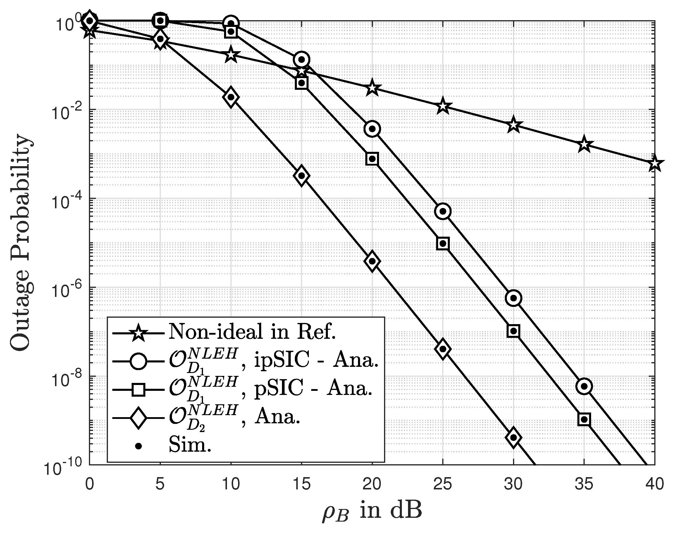
4.2.2. The OP in the Scenario of NLEH

In the scenario of NLEH $\left(\iota <\infty \right)$, the OP at $U_1$ is expressed as follows:

$$\begin{array}{cc}\hfill {\mathcal{O}}_{U_1}^{NLEH}=& 1-\mathrm{Pr}\left({\displaystyle \frac{{\alpha }_2{\rho }_B{\overline{\gamma }}_r}{{\alpha }_1{\rho }_B{\overline{\gamma }}_r+1}}>{\epsilon }_2,{\displaystyle \frac{{\alpha }_1{\rho }_B{\overline{\gamma }}_r}{\delta {\alpha }_2{\rho }_B{\overline{\gamma }}_r+1}}>{\epsilon }_1\right)\hfill \\ \hfill & \times \left[\mathrm{Pr}\left({\displaystyle \frac{{\alpha }_2\chi {\overline{\gamma }}_{0,1}}{{\alpha }_1\chi {\overline{\gamma }}_{0,1}+1}}>{\epsilon }_2,{\displaystyle \frac{{\alpha }_1\chi {\overline{\gamma }}_{0,1}}{\delta {\alpha }_2\chi {\overline{\gamma }}_{0,1}+1}}>{\epsilon }_1,{\left|c_0\right|}^2\le {\mathsf{\Theta }}_4\right)\right.\hfill \\ \hfill & \left.+\mathrm{Pr}\left({\displaystyle \frac{{\alpha }_2\tilde{\chi }{\left|c_1\right|}^2}{{\alpha }_1\tilde{\chi }{\left|c_1\right|}^2+1}}>{\epsilon }_2,{\displaystyle \frac{{\alpha }_1\tilde{\chi }{\left|c_1\right|}^2}{\delta {\alpha }_2\tilde{\chi }{\left|c_1\right|}^2+1}}>{\epsilon }_1,{\left|c_0\right|}^2>{\mathsf{\Theta }}_4\right)\right].\hfill \end{array}$$

(27)

The OP at $U_1$ can be rewritten as follows:

$$\begin{array}{cc}\hfill {\mathcal{O}}_{U_1}^{NLEH}=& 1-\mathrm{Pr}\left({\overline{\gamma }}_R>{\Xi }_{\max }\right)\hfill \\ \hfill & \times \left[\mathrm{Pr}\left({\overline{\gamma }}_{0,1}>{\mathsf{\Theta }}_{\max },{\left|c_0\right|}^2\le {\mathsf{\Theta }}_4\right)+\mathrm{Pr}\left({\left|c_1\right|}^2>{\tilde{\mathsf{\Theta }}}_{\max },{\left|c_0\right|}^2>{\mathsf{\Theta }}_4\right)\right],\hfill \end{array}$$

(28)

where ${\tilde{\mathsf{\Theta }}}_{\max }=\max \left({\displaystyle \frac{{\epsilon }_2}{\tilde{\chi }\left({\alpha }_2-{\epsilon }_2{\alpha }_1\right)}},{\displaystyle \frac{{\epsilon }_1}{\tilde{\chi }\left({\alpha }_1-{\epsilon }_1\delta {\alpha }_2\right)}}\right)$. It is noted that we can rewrite Equation (28) as follows:

$$\begin{array}{cc}\hfill {\mathcal{O}}_{U_1}^{NLEH}=& 1-{\overline{F}}_{{\overline{\gamma }}_r}\left({\Xi }_{\max }\right)\hfill \\ \hfill & \times \left[\left(1-F_{{\overline{\gamma }}_{0,1}}\left({\mathsf{\Theta }}_{\max }\right)\right)\left(1-F_{{\left|c_0\right|}^2}\left({\mathsf{\Theta }}_4\right)\right)+F_{{\left|c_1\right|}^2}\left({\tilde{\mathsf{\Theta }}}_{\max }\right)F_{{\left|c_0\right|}^2}\left({\mathsf{\Theta }}_4\right)\right].\hfill \end{array}$$

(29)

Combining Equations (17) and (22), the OP at $U_1$ with NLEH can be calculated as follows:

$$\begin{array}{cc}\hfill {\mathcal{O}}_{U_1}^{NLEH}=& 1-{\mathcal{Q}}_{{\mu }_r}\left(\sqrt{2{\kappa }_r{\mu }_r},\sqrt{2{\psi }_r{\Xi }_{\max }}\right)\hfill \\ \hfill & \times 〈\left[1-{\displaystyle \frac{1}{{\mathsf{\Phi }}_{0,1}}}\sum _{m=0}^{\infty }\sum _{n=0}^{\infty }{\mathcal{I}}_{0,1}^{n,m}{G}_{1,3}^{2,1}\left({\mathsf{\Theta }}_{\max }{\psi }_0{\psi }_1\left|\begin{array}{c}1\\ m+{\mu }_0,n+{\mu }_1,0\end{array}\right.\right)\right]\hfill \\ \hfill & \times \left[1-{\mathcal{Q}}_{{\mu }_0}\left(\sqrt{2{\kappa }_0{\mu }_0},\sqrt{2{\psi }_0{\mathsf{\Theta }}_4}\right)\right]\hfill \\ \hfill & +{\mathcal{Q}}_{{\mu }_2}\left(\sqrt{2{\kappa }_1{\mu }_1},\sqrt{2{\psi }_1{\tilde{\mathsf{\Theta }}}_{\max }}\right){\mathcal{Q}}_{{\mu }_0}\left(\sqrt{2{\kappa }_0{\mu }_0},\sqrt{2{\psi }_0{\mathsf{\Theta }}_4}\right)〉.\hfill \end{array}$$

(30)

Finally, the OP at $U_2$ with NLEH can be given by:

$$\begin{array}{cc}\hfill {\mathcal{O}}_{U_2}^{NLEH}=& 1-\mathrm{Pr}\left({\displaystyle \frac{{\alpha }_2{\varrho }_B{\overline{\gamma }}_r}{{\alpha }_1{\varrho }_B{\overline{\gamma }}_r+1}}>{\epsilon }_2\right)\left[\mathrm{Pr}\left({\displaystyle \frac{{\alpha }_2\chi {\overline{\gamma }}_{0,2}}{{\alpha }_1\chi {\overline{\gamma }}_{0,2}+1}}>{\epsilon }_2,{\left|h_0\right|}^2\le {\mathsf{\Theta }}_4\right)\right.\hfill \\ \hfill & \left.+\mathrm{Pr}\left({\displaystyle \frac{{\alpha }_2\tilde{\chi }{\left|c_2\right|}^2}{{\alpha }_1\tilde{\chi }{\left|c_2\right|}^2+1}}>{\epsilon }_2,{\left|c_0\right|}^2>{\mathsf{\Theta }}_4\right)\right]\hfill \\ \hfill =& 1-\mathrm{Pr}\left({\overline{\gamma }}_r>{\Xi }_2\right)\hfill \\ \hfill & \times \left[\mathrm{Pr}\left({\overline{\gamma }}_{0,2}>{\mathsf{\Theta }}_2,{\left|c_0\right|}^2\le {\mathsf{\Theta }}_4\right)+\mathrm{Pr}\left({\left|c_2\right|}^2>{\mathsf{\Theta }}_3,{\left|c_0\right|}^2>{\mathsf{\Theta }}_4\right)\right].\hfill \end{array}$$

(31)

We have that Equation (31) is eventually simplified as follows:

$$\begin{array}{cc}\hfill {\mathcal{O}}_{U_2}^{NLEH}=& 1-{\overline{F}}_{{\overline{\gamma }}_r}\left({\Xi }_{\max }\right)\hfill \\ \hfill & \times \left[\left(1-F_{{\overline{\gamma }}_{0,2}}\left({\mathsf{\Theta }}_2\right)\right)\left(1-F_{{\left|c_0\right|}^2}\left({\mathsf{\Theta }}_4\right)\right)+F_{{\left|c_2\right|}^2}\left({\mathsf{\Theta }}_3\right)F_{{\left|c_0\right|}^2}\left({\mathsf{\Theta }}_4\right)\right].\hfill \end{array}$$

(32)

Similarly, by solving for ${\mathcal{O}}_{U_1}^{NLEH}$, ${\mathcal{O}}_{U_2}^{NLEH}$ can be obtained as follows:

$$\begin{array}{cc}\hfill {\mathcal{O}}_{U_2}^{NLEH}=& 1-{\mathcal{Q}}_{{\mu }_r}\left(\sqrt{2{\kappa }_r{\mu }_r},\sqrt{2{\psi }_r{\Xi }_2}\right)\hfill \\ \hfill & \times 〈\left[1-{\displaystyle \frac{1}{{\mathsf{\Phi }}_{0,2}}}\sum _{m=0}^{\infty }\sum _{n=0}^{\infty }{\mathcal{I}}_{0,2}^{n,m}{G}_{1,3}^{2,1}\left({\mathsf{\Theta }}_2{\psi }_0{\psi }_2\left|\begin{array}{c}1\\ m+{\mu }_0,n+{\mu }_2,0\end{array}\right.\right)\right]\hfill \\ \hfill & \times \left[1-{\mathcal{Q}}_{{\mu }_0}\left(\sqrt{2{\kappa }_0{\mu }_0},\sqrt{2{\psi }_0{\mathsf{\Theta }}_4}\right)\right]\hfill \\ \hfill & +{\mathcal{Q}}_{{\mu }_2}\left(\sqrt{2{\kappa }_2{\mu }_2},\sqrt{2{\psi }_2{\mathsf{\Theta }}_3}\right){\mathcal{Q}}_{{\mu }_0}\left(\sqrt{2{\kappa }_0{\mu }_0},\sqrt{2{\psi }_0{\mathsf{\Theta }}_4}\right)〉.\hfill \end{array}$$

(33)

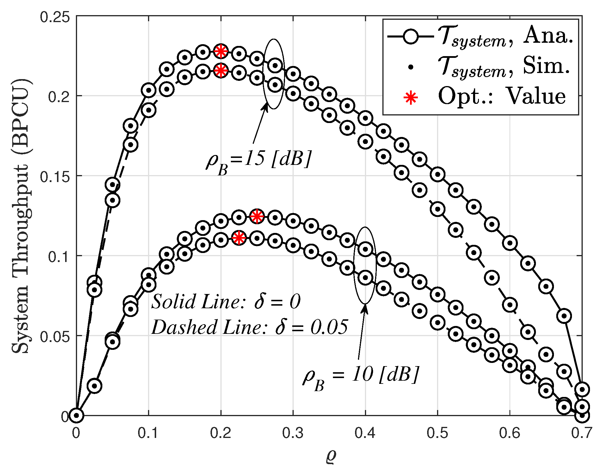
4.3. System Throughput Analysis (STA)

In the delay-limited transmission mode, data are sent from the transmitter R to users at a fixed data rate. During this mode, the transmitter B maintains a steady transmission rate denoted as R, which can be impacted by the occurrence probability of outages owing to fluctuating wireless channel conditions. The relative throughput of the NOMA system is expressed by Equation [22] (Eq. (14)) (refer to (34)).

$$\begin{array}{c}{\mathcal{T}}_{system}={\sum }_{i=1}^2{\displaystyle \frac{\left(1-{\mathcal{O}}_{U_i}^{LEH}\right)\left(1-\varrho \right)T/\phantom{T2}2}{T}}{R}_i={\sum }_{i=1}^2{\displaystyle \frac{\left(1-{\mathcal{O}}_{U_i}^{LEH}\right)\left(1-\varrho \right)R_i}{2}}.\hfill \end{array}$$

(34)

Remark 1. 

Because the cumulative throughput depends on the OPs of $U_i$ and the desired rate $R_i$, it is upper-bounded by the ceiling ${\displaystyle \sum _{i=1}^2}{R}_i$. Moreover, power allocation at both the transmitter B and the relay R also contributes to a decrease in throughput due to their detrimental effects on outage performance.

5. Pseudo Code

To offer a better understanding of the power beacon-assisted scheme, a flowchart outlining the methodology is also provided in Figure 3.

From expression (12), the study presents an algorithm for the Monte Carlo simulation with two users ($U_i$, $i\in \left\{1,2\right\}$), detailed in Algorithm 1.

Algorithm 1: The proposed method for Problem-Solving $\left(\mathcal{P}2\right)$

1. Initialization:    1.1 Set $\overline{\wp }={\displaystyle \frac{\sqrt{5}-1}{2}}$    1.2 Set ${\rho }_{\min }=0$    1.3 Set ${\rho }_{\max }=1-{\displaystyle \frac{2R^2}{{\log }_2\left(1/{\alpha }^2\right)}}$    1.4 Set $\nu ={10}^{-9}$ 2. While Loop:    2.1 while $\left|{\rho }_{\max }-{\rho }_{\min }\right|>\nu$ do:       2.1.1 Set ${\rho }_1={\rho }_{\max }-\left({\rho }_{\max }-{\rho }_{\min }\right)\overline{\wp }$       2.1.2 Set ${\rho }_2={\rho }_{\max }+\left({\rho }_{\max }-{\rho }_{\min }\right)\overline{\wp }$       2.1.3 Obtain ${OLEH}_{U_i}\left({\rho }_1\right)$ from (23) or (25)       2.1.4 Obtain ${OLEH}_{U_i}\left({\rho }_2\right)$ from (23) or (25)       2.1.5   If ${OLEH}_{U_i}\left({\rho }_1\right)>{OLEH}_{U_i}\left({\rho }_2\right)$ then       2.1.5.1   Set ${\rho }_{\max }={\rho }_2$                       else:       2.1.5.2   Set ${\rho }_{\min }={\rho }_1$       2.1.6   end    2.2 End while 3. Return the Optimal ${\rho }^{*}$:    3.1 Return ${\rho }^{*}=\left({\rho }_{\max }+{\rho }_{\min }\right)/\phantom{\left({\rho }_{\max }-{\rho }_{\min }\right)2}2$

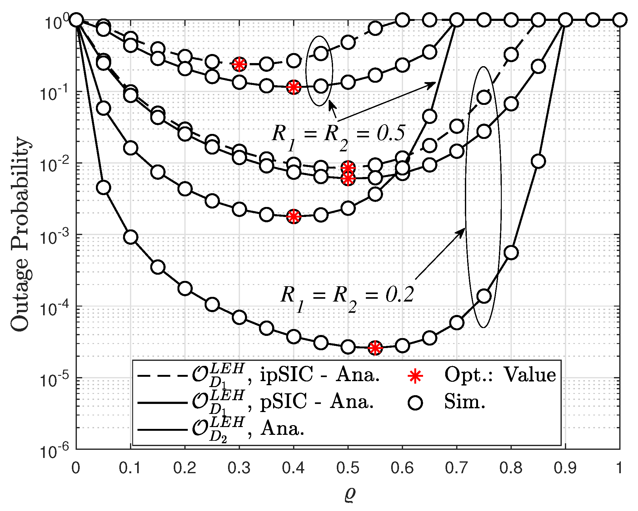
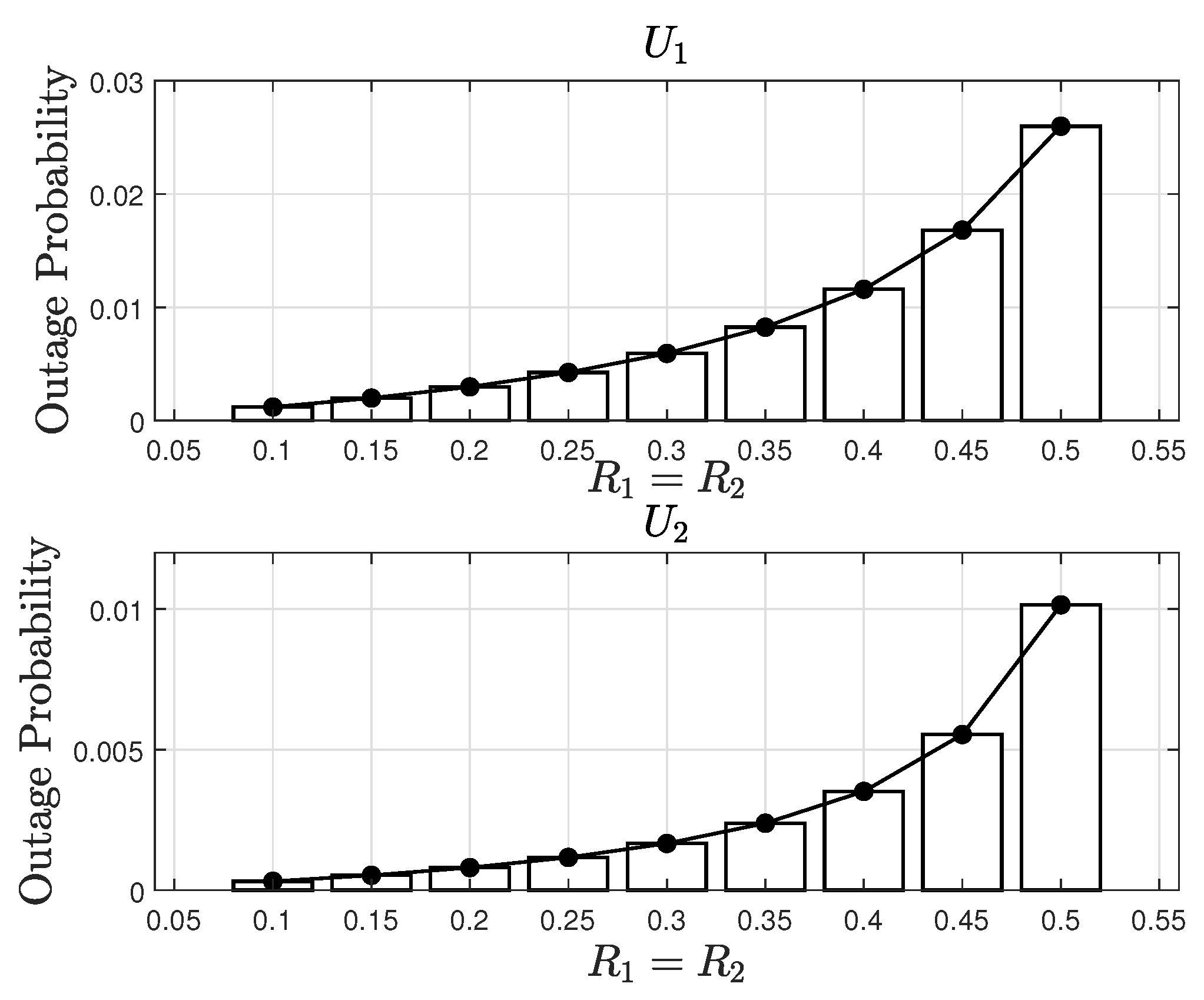
6. Optimization of the TS Factor to Minimize the OP for Users

This section focuses on optimizing the TS factor $\varrho$, which is a crucial parameter for effectively balancing the EH and data transmission phases, aiming to minimize the OP of users. Below is the formula for calculating the OP of users:

$$\begin{array}{c}\left(\mathcal{P}1\right):\underset{\varrho }{\mathrm{minimize}}{\mathcal{O}}_{U_i}^{out},i\in \left\{1,2\right\}\hfill \\ \mathrm{s}.\mathrm{t}.0<\varrho <1-\left[2R_2/\phantom{2R_2{\log }_2\left(1/\phantom{1{\alpha }_2}{\alpha }_2\right)}{\log }_2\left(1/\phantom{1{\alpha }_2}{\alpha }_2\right)\right].\hfill \end{array}$$

(35)

The OP function of $U_i$ versus $\varrho$ exhibits an optimal ${\varrho }^{*}$ on the interval $\left[\tau ,1-\left[2R_2/\phantom{2R_2{\log }_2\left(1/\phantom{1{\alpha }_2}{\alpha }_2\right)}{\log }_2\left(1/\phantom{1{\alpha }_2}{\alpha }_2\right)\right]-\tau \right]\tau \simeq 0$ with $\tau \simeq 0$, similar to references [44,45]. The credibility of these convex function characteristics was validated in [46]. However, no supporting evidence is presented. It is reasonable to reformulate the problem outlined in Equation (35) as follows:

$$\begin{array}{c}\left(\mathcal{P}2\right):\underset{\varrho }{\mathrm{maximize}}-{\mathcal{O}}_{U_i}^{out}\hfill \\ \mathrm{s}.\mathrm{t}.0<\varrho <1-\left[2R_i/\phantom{2R_i{\log }_2\left(1/\phantom{1{\alpha }_2}{\alpha }_2\right)}{\log }_2\left(1/\phantom{1{\alpha }_2}{\alpha }_2\right)\right].\hfill \end{array}$$

(36)

Given the computational challenges associated with employing gradient methods to solve the formula expression $\mathcal{P}2$, we utilize the Golden Section Search technique, as elaborated in Table 2. Here, $\nu$ represents the search accuracy, while $O\left[{\log }_2\left(1/\nu \right)\right]$ indicates the complexity of the method, as stated in the work by Nguyen in [21]. This technique is widely acknowledged for its combination of high precision and low computational complexity, as highlighted by Nguyen. Furthermore, Nguyen demonstrated that for unimodal functions, this method consistently achieves convergence to the global optimum.

7. Energy Efficiency

To enhance throughput in delay-constrained transmission scenarios, further research is crucial to explore the energy efficiency of C-NOMA systems. The necessity for additional studies is highlighted by the reference in [17] (Eq. (52)), which indicates that the formula for the energy efficiency coefficient can yield valuable insights into the performance metrics of these systems. Therefore, examining the details of this coefficient can provide a deeper understanding of how C-NOMA setups can optimize energy consumption while maintaining high throughput levels. The energy efficiency coefficient can be expressed as follows:

$${\eta }_{EE}={\displaystyle \frac{\mathrm{Total}\mathrm{data}\mathrm{rate}}{\begin{array}{c}\mathrm{Total}\mathrm{energy}\mathrm{consumption}\hfill \end{array}}}.$$

(37)

Consequently, the energy efficiency metrics of C-NOMA systems can be redefined as follows:

$${\eta }_{system}^{EE}={\displaystyle \frac{{\mathcal{T}}_{system}}{T{P}_B+T{P}_R}},$$

(38)

In this context, the variable T represents the duration of the transmission procedure, covering all aspects of the communication process.

8. Simulation Results

In this section, we evaluate the OP and throughput of the proposed system through analytical analysis, supplemented by simulation results obtained using the Monte Carlo method to validate our analytical findings. The parameters of the $\kappa -\mu$ random variables are assumed to be identical, namely $\kappa ={\kappa }_R={\kappa }_0={\kappa }_1={\kappa }_2$ and $\mu ={\mu }_R={\mu }_0={\mu }_1={\mu }_2$, with $\mathsf{\Omega }={\mathsf{\Omega }}_R={\mathsf{\Omega }}_0={\mathsf{\Omega }}_1={\mathsf{\Omega }}_2=1$. Unless otherwise stated, all simulation configurations are provided in

Table 4. Definition of system parameters.

Parameters	Notations	Values
Power splitting factors	$\left\{{\alpha }_1,{\alpha }_2\right\}$	$\left\{0.3,0.7\right\}$
Threshold data rate at $U_1$	$R_1$	$0.5$ Bit/s/Hz
Threshold data rate at $U_2$	$R_2$	$0.25$ Bit/s/Hz
Time-switching factor	$\varrho$	$0.5$
Coherence time block	T	1
Interference factor	$\delta$	$0.05$
Energy conversion efficiency	$\eta$	$0.8$
Monte-Carlo sample	−	${10}^6$

. Moreover, we employed the $\kappa -\mu$ fading model, and a variety of examples can be found in

Table 5. The $\kappa -\mu$ distribution yields common fading distributions [48].

Channels	$\mathit{\kappa }-\mathit{\mu }$ Distribution Parameters
Rayleigh	$\mu =1$, $\kappa \to 0$
One-sided Gaussian	$\mu =0.5$, $\kappa \to 0$
Nakagami-m	$\mu =m$, $\kappa \to 0$
Rician with parameter K	$\mu =1$, $\kappa =K$
$\kappa -\mu$	$\mu =\mu$, $\kappa =\kappa$

. For scenarios involving NLEH, we set $\iota =0$ dBm and $N_0=-90$ dBm as specified in [47].

The two $\kappa -\mu$ random variables associated with the EH-NOMA system discussed in Section 3 are clearly depicted in Figure 4. This visualization illustrates that the simulation outcomes closely align with the numerical analysis we conducted, which was derived from simulation data.

Figure 5 shows the representation of OP according to ${\rho }_B$ in a cooperative NOMA system with different $\kappa$ and $\mu$ values. Specifically, Figure 5a presents the OP of the Rice distribution ($\mu =1$) versus two values $\kappa =1$ and $\kappa =4$. From the figure, it can be observed that the larger the $\kappa$, the better the OP of the system. A similar explanation is provided for Figure 5b for the Nakagami-m distribution ($\kappa \to 0$) versus two values $\mu =1$ and $\mu =3$. From the figure, we can also see that the larger the value of $\mu$, the lower the OP. These results can be explained based on Equations (23)–(26). Generally, the alignment between simulation results and analytical results in NOMA systems can be attributed to several key factors: accurate user pairing, optimized power allocation, and precise interference management through SIC. These elements collectively enhance the predictability and stability of the channel environment, ensuring that theoretical models closely match simulations.

Figure 6 findings are identical to Figure 5 in terms of general channel characteristics; we can see that for the situation, NLEH will be better than LEH, as shown in Figure 5.

The the OP values for $U_1$ and $U_2$ as a function of ${\rho }_B$ are presented in Figure 7a and Figure 7b respectively. The figure reveals that the Nakagami-m distribution has the lowest OP value, while the One-sided Gaussian distribution has the highest OP value. This suggests that the transmission line with the Nakagami-m distribution is the most stable. This observation can also be explained using Equations (23)–(26).

Upon applying NLEH, an enhancement in outage performance for the downlink scenario is apparent in Figure 8. Here, we set $\delta =0.05$. It is notable that as the SNR ${\rho }_B$ during transmission increases, a considerable gap emerges between the outage probabilities attained by the linear and non-linear EH models. This disparity arises due to the extended duration required for EH to accumulate the minimum power influenced by $\iota$, consequently diminishing the OP.

Figure 9 illustrates OP versus the power allocation factor $a_2$, where a larger value of ${\rho }_B$ indicates better optimization. Based on the figure, we observe that the OP occurs at $U_1$ when the ipSIC ceases to function entirely within the ${\alpha }_2$ range from 0.86 to 1. Similarly, the OP occurs at $U_1$ in the case of pSIC complete outage within the ${\alpha }_2$ range from 0.97 to 1. These observations can be explained similarly to Figure 3 and Figure 4, as well as based on Equations (23)–(26).

Figure 10 plots the OP versus $\varrho$ for various target rate values, with parameters $\delta =0.02$, ${\alpha }_1=0.1$, ${\alpha }_2=0.9$, $\kappa =0$, and $\mu =3$. Specifically, as the target rate values change from $R_1=R_2=0.2$ to $R_1=R_2=0.5$, the OP also increases. We can explain these observations based on Equations (23)–(26).

Figure 11 describes the OP at $U_1$ and $U_2$ versus target rate values ($R_1=R_2$). Specifically, the figure illustrates that OP increases with increasing target rate values.

Figure 12 illustrates the ST at the destination node versus $\varrho$, where $R_1=0.5$, $R_2=0.25$, ${\alpha }_1=0.3$, ${\alpha }_2=0.7$, $\kappa =0$, and $\mu =2$. The exact theoretical curves of the system throughput are plotted according to Equation (21). From the graph, it is evident that the system throughput increases as the value of ${\rho }_B$ increases. When ${\rho }_B$ changes from 10 [dB] to 15 [dB], the maximum system throughput nearly doubles. Additionally, the system throughput is dependent on $\delta$, with $\delta =0$ corresponding to the dashed line and $\delta =0.05$ corresponding to the solid line. As $\delta$ increases at the same value of ${\rho }_B$, the system throughput decreases rapidly, and vice versa. This implies that the quality of the system is dependent on the quality of the SIC.

In Figure 13, we adjust the simulation settings to match those in [36], and the outage probability of an energy harvesting-based NOMA system falls dramatically in the high SNR zone. Such patterns in outage performance are observed for both time switching and power splitting systems, which are consistent with our findings. However, target rates remain a restriction of our proposed system’s outage performance, as indicated in [36]. It is concluded that our relay-based NOMA system outperforms that of [36] in terms of outage performance in the case of time-switching energy harvesting at SNRs greater than 20 dB.

We show the outage probability at the users versus $\rho$ for the LEH and NLEH cases in Figure 14. It can be noted that when $\rho$ increases, the NOMA system’s outage performance improves. This is because a greater $\rho$ corresponds to a higher diversity order for each user, resulting in a reduced outage probability. Furthermore, the study in Figure 8 shows that the users in the NLEH scenario outperform those in the LEH case.

Figure 15 illustrates the relationship between system energy efficiency and SNR when operating in delay-limited transmission mode for user relaying within NOMA systems. The plotted graph includes dashed curves representing the performance of two users relaying NOMA with the LEH scenario, derived from Equations (24) and (26) based on throughput in delay-limited transmission mode. Additionally, solid curves on the graph depict the results for two users relaying NOMA with the NLEH setup, calculated using Equations (A1) and (A4) considering throughput in transmission mode.

Upon observation, it becomes apparent that the energy efficiency of user relaying in NLEH NOMA during delay-limited transmission mode exhibits a higher throughput compared to that of LEH NOMA under similar transmission conditions. Through the comparison of these scenarios, it is evident that the NLEH configuration offers improved energy efficiency for user relaying within NOMA systems, particularly in delay-limited transmission mode. The findings from the plotted curves emphasize the advantages of utilizing NLEH over LEH in terms of energy efficiency and throughput performance when implementing user relaying in NOMA systems. This insight underscores the significance of considering different energy harvesting mechanisms in NOMA setups to enhance system performance and efficiency.

9. Conclusions

This paper investigates the DF relay-based protocol for EH and IP in wireless C-NOMA relaying networks. We derived closed-form expressions for the OP, ST, and the optimal TS factor to minimize OP for two users. Additionally, expressions for achievable OP, ST, and the optimal TS factor for users of the TSR protocol for SWIPT were obtained. Analytical and simulation results consistently demonstrate the superiority of the Nakagami-m fading channel over other fading channels in terms of energy efficiency performance. For instance, simulations with parameters such as $\kappa =0$, $\mu =3$, and SNR ranging from 10 dB to 20 dB showed up to 20% lower outage probabilities compared to Rice and One-sided Gaussian channels. Despite these promising findings, our study is not without limitations. One limitation is the assumption of identical parameters ($\kappa ={\kappa }_R={\kappa }_0={\kappa }_1={\kappa }_2$ and $\mu ={\mu }_R={\mu }_0={\mu }_1={\mu }_2$) across different scenarios, which may not fully capture real-world variations in channel conditions. Additionally, while our simulations provide valuable insights, they are based on specific configurations and may not generalize to all practical deployment scenarios. Moving forward, we propose the development of a C-NOMA network system utilizing multiple-input-multiple-output (MIMO) NOMA to further enhance system performance and address these limitations. This avenue presents promising opportunities for future research and practical implementation, aiming to optimize wireless communication networks through advanced NOMA techniques.

References

1. Dai, L.; Wang, B.; Ding, Z.; Wang, Z.; Chen, S.; Hanzo, L. A Survey of Non-Orthogonal Multiple Access for 5G. IEEE Commun. Surv. Tutor. 2018, 20, 2294–2323. [Google Scholar] [CrossRef]
2. Makki, B.; Chitti, K.; Behravan, A.; Alouini, M.-S. A Survey of NOMA: Current Status and Open Research Challenges. IEEE Open J. Commun. Soc. 2020, 1, 179–189. [Google Scholar] [CrossRef]
3. Al-habob, A.A.; Salhab, A.M.; Zummo, S.A. A Novel Time-Switching Relaying Protocol for Multi-user Relay Networks with SWIPT. Arab. J. Sci. Eng. 2019, 44, 2253–2263. [Google Scholar] [CrossRef]
4. Tran, H.Q.; Phan, C.V.; Vien, Q.T. Power splitting versus time switching based cooperative relaying protocols for SWIPT in NOMA systems. Phys. Commun. 2020, 41, 101098. [Google Scholar] [CrossRef]
5. Tran, H.Q.; Phan, C.V.; Vien, Q.T. Performance analysis of power-splitting relaying protocol in SWIPT based cooperative NOMA systems. EURASIP J. Wirel. Commun. Netw. 2021, 2021, 110. [Google Scholar] [CrossRef]
6. Tran, H.Q.; Vien, Q.T. SWIPT-Based Cooperative NOMA for Two-Way Relay Communications: PSR versus TSR. Wirel. Commun. Mob. Comput. 2023, 2023, 3069999. [Google Scholar] [CrossRef]
7. Alhamad, R.; Boujemaa, H. Non Orthogonal Multiple Access for Multi-carrier Code Division Multiple Access Systems with Energy Harvesting. Wirel. Pers. Commun. 2024, 134, 2121–2136. [Google Scholar] [CrossRef]
8. Ogundokun, R.O.; Awotunde, J.B.; Imoize, A.L.; Li, C.-T.; Abdulahi, A.T.; Adelodun, A.B.; Sur, S.N.; Lee, C.-C. Non-Orthogonal Multiple Access Enabled Mobile Edge Computing in 6G Communications: A Systematic Literature Review. Sustainability 2023, 15, 7315. [Google Scholar] [CrossRef]
9. Islam, S.M.; Avazov, N.; Dobre, O.A.; Kwak, K.S. Power-Domain Non-Orthogonal Multiple Access (NOMA) in 5G Systems: Potentials and Challenges. IEEE Commun. Surv. Tutor. 2017, 19, 721–742. [Google Scholar] [CrossRef]
10. Dai, L.; Wang, B.; Yuan, Y.; Han, S.; I, C.L.; Wang, Z. Non-orthogonal multiple access for 5G: Solutions, challenges, opportunities, and future research trends. IEEE Commun. Mag. 2015, 53, 74–81. [Google Scholar] [CrossRef]
11. Tran, H.Q.; Truong, P.Q.; Phan, C.V.; Vien, Q.T. On the energy efficiency of NOMA for wireless backhaul in multi-tier heterogeneous CRAN. In Proceedings of the 2017 International Conference on Recent Advances in Signal Processing, Telecommunications & Computing (SigTelCom), Da Nang, Vietnam, 9–11 January 2017; pp. 229–234. [Google Scholar] [CrossRef]
12. Sur, S.N.; Kandar, D.; Silva, A.; Nguyen, N.D.; Nandi, S.; Do, D.-T. Hybrid Precoding Algorithm for Millimeter-Wave Massive MIMO-NOMA Systems. Electronics 2022, 11, 2198. [Google Scholar] [CrossRef]
13. Ding, Z.; Lei, X.; Karagiannidis, G.K.; Schober, R.; Yuan, J.; Bhargava, V.K. A Survey on Non-Orthogonal Multiple Access for 5G Networks: Research Challenges and Future Trends. IEEE J. Sel. Areas Commun. 2017, 35, 2181–2195. [Google Scholar] [CrossRef]
14. Tsiropoulos, G.I.; Yadav, A.; Zeng, M.; Dobre, O.A. Cooperation in 5G HetNets: Advanced Spectrum Access and D2D Assisted Communications. IEEE Wirel. Commun. 2017, 24, 110–117. [Google Scholar] [CrossRef]
15. Zhang, Z.; Ma, Z.; Xiao, M.; Ding, Z.; Fan, P. Full-duplex device-to-device-aided cooperative nonorthogonal multiple access. IEEE Trans. Veh. Technol. 2017, 66, 4467–4471. [Google Scholar] [CrossRef]
16. Wang, Z.; Yue, X.; Peng, Z. Full-duplex user relaying for NOMA system with self-energy recycling. IEEE Access 2018, 6, 67057–67069. [Google Scholar] [CrossRef]
17. Yue, X.; Liu, Y.; Kang, S.; Nallanathan, A.; Ding, Z. Exploiting Full/Half-Duplex User Relaying in NOMA Systems. IEEE Trans. Commun. 2018, 66, 560–575. [Google Scholar] [CrossRef]
18. Abbasi, O.; Ebrahimi, A. Cooperative NOMA with full-duplex amplify-and-forward relaying. Trans. Emerg. Telecommun. Technol. 2018, 29, e3421. [Google Scholar] [CrossRef]
19. Yang, Z.; Ding, Z.; Wu, Y.; Fan, P. Novel Relay Selection Strategies for Cooperative NOMA. IEEE Trans. Veh. Technol. 2017, 66, 10114–10123. [Google Scholar] [CrossRef]
20. Duan, W.; Ju, J.; Hou, J.; Sun, Q.; Jiang, X.Q.; Zhang, G. Effective resource utilization schemes for decode-and-forward relay networks with NOMA. IEEE Access 2019, 7, 51466–51474. [Google Scholar] [CrossRef]
21. Doan, T.B.; Nguyen, T.H. Exploiting SWIPT for Coordinated-NOMA Systems Under Nakagami-m Fading. IEEE Access. 2024, 12, 19216–19228. [Google Scholar] [CrossRef]
22. Nasir, A.A.; Zhou, X.; Durrani, S.; Kennedy, R.A. Relaying Protocols for Wireless Energy Harvesting and Information Processing. IEEE Trans. Wirel. Commun. 2013, 12, 3622–3636. [Google Scholar] [CrossRef]
23. Dubey, S.; Mehra, N.; Shakya, D.K. Time and relay shared full/half duplex cooperative NOMA with paired cell edge users. AEU-Int. J. Electron. Commun. 2024, 177, 155168. [Google Scholar] [CrossRef]
24. Chu, T.M.C.; Zepernick, H.J. Performance of a Non-Orthogonal Multiple Access System with Full-Duplex Relaying. IEEE Commun. Lett. 2018, 22, 2084–2087. [Google Scholar] [CrossRef]
25. Mohammadi, M.; Chalise, B.K.; Hakimi, A.; Suraweera, H.A.; Ding, Z. Joint Beamforming Design and Power Allocation for Full-Duplex NOMA Cognitive Relay Systems. In Proceedings of the 2017 IEEE Global Communications Conference, Singapore, 4–8 December 2017; pp. 1–6. [Google Scholar] [CrossRef]
26. Guo, C.; Zhao, L.; Feng, C.; Ding, Z.; Wang, H.-M. Secrecy Performance of NOMA Systems With Energy Harvesting and Full-Duplex Relaying. IEEE Trans. Veh. Technol. 2020, 69, 12301–12305. [Google Scholar] [CrossRef]
27. Guo, C.; Zhao, L.; Feng, C.; Ding, Z.; Chen, H.-H. Energy Harvesting Enabled NOMA Systems With Full-Duplex Relaying. IEEE Trans. Veh. Technol. 2019, 68, 7179–7183. [Google Scholar] [CrossRef]
28. Singh, C.K.; Upadhyay, P.K. Overlay Cognitive IoT-Based Full-Duplex Relaying NOMA Systems With Hardware Imperfections. IEEE Internet Things J. 2022, 9, 6578–6596. [Google Scholar] [CrossRef]
29. Rauniyar, A.; Engelstad, P.E.; Østerbø, O.N. On the Performance of Bidirectional NOMA-SWIPT Enabled IoT Relay Networks. IEEE Sens. J. 2021, 21, 2299–2315. [Google Scholar] [CrossRef]
30. Sixtus J, R.J.; Muthu, T. Investigations on IoT with SWIPT-NOMA Combination in Wireless Sensor Networks. In Proceedings of the 2022 International Conference on Inventive Computation Technologies (ICICT), Lalitpur, Nepal, 20–22 July 2022; pp. 688–693. [Google Scholar] [CrossRef]
31. Shaheen, E.M.; Soleymani, M.R. Performance Analyses of SWIPT-NOMA Enabled IoT Relay Networks. In Proceedings of the 2022 International Symposium on Networks, Computers and Communications (ISNCC), Shenzhen, China, 19–22 July 2022; pp. 1–6. [Google Scholar] [CrossRef]
32. Al-Obiedollah, H.; Salameh, H.B.; Gharaibeh, A.; Cumanan, K.; Ding, Z.; Dobre, O.A. Harvested Power Fairness-Based Multi-Carrier NOMA IoT Networks With SWIPT. IEEE Wirel. Commun. Lett. 2023, 12, 381–385. [Google Scholar] [CrossRef]
33. Do, D.-T.; Le, C.-B.; Afghah, F. Enabling Full-Duplex and Energy Harvesting in Uplink and Downlink of Small-Cell Network Relying on Power Domain Based Multiple Access. IEEE Access 2020, 8, 142772–142784. [Google Scholar] [CrossRef]
34. Do, D.-T.; Le, C.-B.; Le, A.-T. Joint of full-duplex relay, non-linear energy harvesting and multiple access in performance improvement of cell-edge user in heterogeneous networks. Wirel. Netw. 2020, 26, 6253–6266. [Google Scholar] [CrossRef]
35. Babaei, M.; Aygolu, U.; Basar, E. Cooperative AF relaying with energy harvesting in Nakagami- fading channel. Phys. Commun. 2019, 34, 105–113. [Google Scholar] [CrossRef]
36. Li, X.; Huang, M.; Zhang, C.; Deng, D.; Rabie, K.M.; Ding, Y.; Du, J. Security and Reliability Performance Analysis of Cooperative Multi-Relay Systems With Nonlinear Energy Harvesters and Hardware Impairments. IEEE Access 2019, 7, 102644–102661. [Google Scholar] [CrossRef]
37. Le, A.-T.; Tran, D.-H.; Le, C.-B.; Tin, P.T.; Nguyen, T.N.; Ding, Z.; Poor, H.V.; Voznak, M. Power Beacon and NOMA-Assisted Cooperative IoT Networks With Co-Channel Interference: Performance Analysis and Deep Learning Evaluation. IEEE Trans. Mob. Comput. 2024, 23, 7270–7283. [Google Scholar] [CrossRef]
38. Solanki, S.; Upadhyay, P.K.; da Costa, D.B.; Ding, H.; Moualeau, J.M. Performance analysis of piece-wise linear model of energy harvesting-based multiuser overlay spectrum sharing networks. IEEE Open J. Commun. Soc. 2020, 1, 1820–1836. [Google Scholar] [CrossRef]
39. Gradshteyn, I.S.; Ryzhik, I.M. Table of Integrals, Series and Products, 7th ed.; Academic: San Diego, CA, USA, 2007. [Google Scholar]
40. Karagiannidis, G.K.; Sagias, N.C.; Mathiopoulos, P.T. N–Nakagami: A novel stochastic model for cascaded fading channels. IEEE Trans. Commun. 2007, 55, 1453–1458. [Google Scholar] [CrossRef]
41. Nadarajah, S. Exact distribution of the product of m gamma and n Pareto random variables. J. Comput. Appl. Math. 2011, 235, 4496–4512. [Google Scholar] [CrossRef]
42. Simon, M.K.; Alouini, M.-S. Digital Communication over Fading Channels; John Wiley & Sons: Hoboken, NJ, USA, 2005. [Google Scholar]
43. Weisstein, E. Regularized Hypergeometric Function, 3rd ed.; Wolfram Research, Inc.: Champaign, IL, USA, 2003. [Google Scholar]
44. Rauniyar, A.; Engelstad, P.; Østerbø, O.N. RF energy harvesting and information transmission in IoT relay systems based on time switching and NOMA. In Proceedings of the 2018 28th International Telecommunication Networks and Applications Conference (ITNAC), Sydney, NSW, Australia, 21–23 November 2018; pp. 1–7. [Google Scholar] [CrossRef]
45. Rauniyar, A.; Engelstad, P.E.; Østerbø, O.N. Performance analysis of RF energy harvesting and information transmission based on NOMA with interfering signal for IoT relay systems. IEEE Sens. J. 2019, 19, 7668–7682. [Google Scholar] [CrossRef]
46. Pei, L.; Yang, Z.; Pan, C.; Huang, W.; Chen, M.; Elkashlan, M.; Nallanathan, A. Energy-efficient D2D communications underlaying NOMA-based networks with energy harvesting. IEEE Commun. Lett. 2018, 22, 914–917. [Google Scholar] [CrossRef]
47. Le-Thanh, T.; Ho-Van, K. Performance Analysis of Wireless Communications with Nonlinear Energy Harvesting under Hardware Impairment and κμ Shadowed Fading. Sensors 2023, 23, 3619. [Google Scholar] [CrossRef]
48. Paris, J.F. Statistical Characterization of κμ Shadowed Fading. IEEE Trans. Veh. Technol. 2014, 63, 518–526. [Google Scholar] [CrossRef]
49. Yacoub, M. The κμ distribution and the ημ distribution. IEEE Antennas Propag. Mag. 2007, 49, 68–81. [Google Scholar] [CrossRef]
Figure 1. System model.
Mathematics 12 02249 g001
Figure 2. A time-power EH Scheme.
Mathematics 12 02249 g002
Figure 3. The flowchart for calculating the primary system metrics for the power beacon-assisted scheme.
Mathematics 12 02249 g003
Figure 4. Visualization of the derived closed-form expression for the PDF and CDF, alongside the graphical representation of the predicted actual distributions.
Mathematics 12 02249 g004
Figure 5. OP versus ρ B with LEH for the Cooperative NOMA system with varying κ and μ values.
Mathematics 12 02249 g005
Figure 6. OP versus ρ B with NLEH for the Cooperative NOMA system with different κ and μ values.
Mathematics 12 02249 g006
Figure 7. OP of U 1 and U 2 versus ρ B for different fading channels, with δ = 0.1 .
Mathematics 12 02249 g007
Figure 8. Comparison performance related to downlink between NLEH and LEH case, with δ = 0.05 .
Mathematics 12 02249 g008
Figure 9. OP versus power allocation factors, with the parameters δ = 0.05 , κ = 3 , and μ = 1 .
Mathematics 12 02249 g009
Figure 10. The OP versus ϱ for different target rate values, with the parameters δ = 0.02 , α 1 = 0.1 , α 2 = 0.9 , κ = 0 , and μ = 3 .
Mathematics 12 02249 g010
Figure 11. The OP versus the target rates, with the parameters δ = 0.05 , α 1 = 0.2 , α 2 = 0.8 , κ = 3 , and μ = 1 .
Mathematics 12 02249 g011
Figure 12. The ST at the destination node with respect to ϱ , with the parameters R 1 = 0.5 , R 2 = 0.25 , α 1 = 0.3 , α 2 = 0.7 , κ = 0 , and μ = 2 .
Mathematics 12 02249 g012
Figure 13. A comparison of the results presented in [36] regarding outage probability, with the parameters R 1 = 0.5 , R 2 = 0.25 , α 1 = 0.3 , α 2 = 0.7 , κ = 0 , and μ = 4 .
Mathematics 12 02249 g013
Figure 14. The outage probabilities at the other users versus ρ B .
Mathematics 12 02249 g014
Figure 15. System energy efficiency in delay-limited transmission mode, where a 1 = 0.1 , a 2 = 0.9 , κ = 4 , μ = 1 , P B = P R = 10 W and T = 1 .
Mathematics 12 02249 g015