Abstract
When using multi-criteria decision-making methods in applied problems, an important aspect is the determination of the criteria weights. These weights represent the degree of each criterion’s importance in a certain group. The process of determining weight coefficients from a dataset is described as an objective weighting method. The dataset considered here contains quantitative data representing measurements of the alternatives being compared, according to a previously determined system of criteria. The purpose of this study is to suggest a new method for determining objective criteria weights and estimating the proximity of the studied criteria to the centres of their groups. It is assumed that the closer a criterion is to the centre of the group, the more accurately it describes the entire group. The accuracy of the description of the entire group’s priorities is interpreted as the importance, and the higher the value, the more significant the weight of the criterion. The Centroidous method suggested here evaluates the importance of each criterion in relation to the centre of the entire group of criteria. The stability of the Centroidous method is examined in relation to the measures of Euclidean, Manhattan, and Chebyshev distances. By slightly modifying the data in the original normalised data matrix by 5% and 10% 100 and 10,000 times, stability is examined. A comparative analysis of the proposed Centroidous method obtained from the entropy, CRITIC, standard deviation, mean, and MEREC methods was performed. Three sets of data were generated for the comparative study of the methods, as follows: the mean value for alternatives with weak and strong differences and criteria with linear dependence. Additionally, an actual dataset from mobile phones was also used for the comparison.
Keywords:
MCDM; Centroidous; objective weighting method; objective weights; criteria; quantitative data; measurements MSC:
68W99; 65Z99; 15-11; 90-08; 68N30
1. Introduction
Multi-criteria decision-making (MCDM) methods have been used for applied problems, alongside other statistical algorithms and machine learning techniques, as illustrated by the number of research publications on this topic in the Web of Science scientific database [1]. Over the period of January 2022 to March 2024, a total of 4132 research papers were published in scientific journals, including survey research articles describing decision-making methods. MCDM methods are preferable in the context of small datasets.
Depending on the nature of the data, subjective or objective methods of determining weight coefficients can be applied; however, regardless of the MCDM method chosen, the condition that the sum of the criteria weights is equal to one remains constant. It should be noted that a subjective method involves expert assessments, whereas an objective method analyses quantitative data. An objective approach analyses the properties of the alternatives under study, such as the measurements, values of technological parameters, duration of the process (time), and cost [2].
In some decision-making situations, extracting subjective preferences is either difficult or inappropriate [3]. According to Pala, when a decision-maker lacks the relevant experience and has no established point of view regarding the aspect of the problem to be solved, objective weights may be advisory rather than mandatory [4].
The range of methods that have been used to study the data structure in order to obtain objective criteria weights is wide and diverse. Objective weights are calculated using the criterion importance through inter criterion correlation (CRITIC) method, which highlights the intensity of the contrast between the presentation of alternatives according to a certain criterion and the conflict of estimation of the contradictory nature of the criteria. The contrast intensity of the corresponding criterion is characterised by a standard deviation [3]. The modelling of the contradictory relationships between the criteria in the CRITIC method has been improved by Krishnan et al. using distance correlation in the distance-CRITIC (D-CRITIC) method [5]. The correlation coefficient and standard deviation (CCSD) method applies an integrated approach to the standard deviation and correlation coefficient [6]. The authors of the CRITIC-M method, Žižović et al., suggest changing the normalisation in CRITIC, arguing that this leads to lower standard deviation values and new insights into the data in the original decision matrix [7]. Statistical measures of standard deviation are applied in the simultaneous evaluation of criteria and alternatives (SECA) method to describe supporting points by studying the variation within and between criteria. This multipurpose nonlinear mathematical model aims to maximise the overall efficiency of each alternative while minimising the deviation of the criteria weights from the supporting points. The SECA method simultaneously calculates general estimates of the effectiveness of the alternatives and criteria weights [8]. The robustness, correlation, and standard deviation (ROCOSD) method distributes weight values with the aim of minimising the total maximum deviation from the ratio of criteria using calculated standard deviations and correlation coefficients [4]. The simple statistical variance method (SV) is also applied to determine the objective criteria weights [9].
The indicator of entropy is often applied to measure the discrepancy in the estimates [4]. As a rule, the concept of uncertainty is considered a synonym for the term entropy [10]. The entropy method was introduced in 1947 by scientists Shannon and Weaver and was later highlighted by Zeleny [11]. Entropy is an important concept in both the social and physical sciences. Podvezko et al. reported that the entropy method was one of the most popular objective methods in the group, as it represents the degree of heterogeneity of criteria values [12]. It has been found that the lower the entropy of a criterion, the more valuable information it contains [11,13]. The integrated approach of entropy-correlated criterion (EWM-CORR) allows for the redistribution of the weights obtained using the entropy method for correlating criteria [13].
The method based on the removal effects of criteria (MEREC) studies the impact of removing each criterion on the effectiveness of the alternatives, which is determined using a simple logarithmic indicator with equal weights [14]. The logarithmic percentage change-driven objective weighting (LOPCOW) method calculates the mean square value of each criterion as a percentage of its standard deviation. The values of the criteria are standardised using min–max normalisation [15]. The CILOS method takes into account the loss of each criterion’s effect when one of the other criteria receives its optimal (highest or lowest) value [16].
Odu has pointed out that neither the subjective nor the objective approaches are ideal. The integrated method of estimating weights overcomes the shortcomings inherent in both approaches and may therefore be the most appropriate for determining the weight coefficients of the criteria [17]. The integrated determination of objective criteria weights (IDOCRIW) method takes into account the integrated estimation of the objective weights of several methods and considers the characteristics of the entropy and CILOS methods [16]. To recalculate the criteria weights based on a combination of subjective and objective views, the Bayes’ theorem has been applied [18]. To reduce the subjectivity of peer assessments, continuous cases of Bayes’ rule were applied using the accumulated experience of assessments expressed by a prior probability distribution. Each assessment is adjusted based on the function of the average posterior probability, according to the expert’s competence [19]. Mukhametzyanov has also expressed support for comprehensive assessment while voicing concerns about the objectivity of assessments made in a technically established way and has highlighted the problems arising from different data structures and the degree of uncertainty. This researcher stressed the importance of a preliminary analysis of the results when choosing the final solution, with due attention to the specific aspects of the applied problem [13]. In some cases, when it can be assumed that all criteria are of equal importance, weights are calculated using the mean weight (MW) method [20]. When there is a large number of criteria, they are usually broken down into smaller subgroups of criteria (from five to seven criteria) [2] to form a hierarchy or system of criteria. Proper structuring of complex issues and explicit consideration of various rules result in better-informed and more effective solutions [21].
Statistics generated for the entire time using the Web of Science scientific database [1] indicate that the 10 most popular areas for the use of objective assessment methods are as follows: medicine (general, internal), clinical neurology, surgery, public environmental occupational health, electrical and electronic engineering, obstetrics and gynaecology, pharmacology, pharmacy, psychiatry, paediatrics, and oncology.
Distance is a fundamental concept in machine learning and neural networks because it enables one to assess the degree of similarity or difference between objects. Euclidean distance is the most preferred measure of distance in practice [22]. Other distance measures include Minkowski, Manhattan (“Taxicab norm” or “City-block”), cosine, Chebyshev (“Maximum Value”, “Lagrange”, and “Chessboard”), Hellinger, angular, Kullback–Leibler, etc. [22,23]. The use of distance is common in various areas of machine learning, including regression, classification, and clustering. Methods, for instance, support vector machine (SVM) for regression problems [24] and classification [25] and the singular value decomposition method (SVD) [26,27], as well as neural networks, in which distance is used as a loss function [28], actively use distance measures. Distances are employed in automatic recommender systems [29] to assess the similarity between rating vectors.
In machine learning, the process of breaking down a dataset into subsets with the same characteristics is called clustering. A clustering method aims to ensure that objects in one subset are not similar to objects in other subsets [30], in which the subsets are called clusters or groups. The most popular non-hierarchical clustering method is K-means, as it uses a simple and rapid approach to data processing [31]. This method was developed by MacQueen in 1967 [32]. The value of K indicates the number of groups into which the objects are to be broken down and is pre-determined by an expert. The K-means algorithm minimises the sum of the distances from each of the objects to their cluster centres [33]. In the classic version, the cluster centre, or centroid, is calculated as the average value of the objects. Each data object is assigned to a cluster based on proximity to the cluster centre, in which proximity is usually measured by the Euclidean distance [31].
This research article suggests a new MCDM method for determining criteria weights by estimating a data array. The importance of criteria is evaluated in relation to the centre of the entire group of criteria. It is assumed that the closer the criterion is to the centre of the group, the more accurately it describes the entire group. This concept is also applied in the case of clustering, since the similarity between the objects is inversely proportional to the distance between them, so the greater the degree of similarity, the smaller the distance [31]. The accuracy of the description of the entire group’s priorities is interpreted as the importance or weight of the criterion.
Although the suggested Centroidous method and the K-means method are similar, they differ greatly from one another. The main difference is the method’s intended use. K-means divides the objects into an optimal number of clusters with similar characteristics; the elbow or ilhouette methods are frequently used to determine the number of clusters [34]. The MCDM Centroidous method, in turn, sets the weights of the criteria, bearing in mind that within the task statement’s structure, the hierarchy of criteria has already been established. The weights in each of the distinct criterion subgroups are determined by the Centroidous. Accordingly, the implementation of the methods differs, and since grouping objects into clusters is a repetitive process, K-means must be programmed. Programming is not necessary to determine the weights of the criterion while using the Centroidous method. After a literature review of MCDM methods, it was determined that the Centroidous method is a novel way to determine the objective weights of criteria.
The theoretical foundation of the proposed Centroidous method repeats the mathematical explanation of other algorithms. According to this method, the core elements that are more important in the context of this group are accumulated in the centre of the group of criteria. The Centroidous method’s logic is predicated on the idea that a criterion’s weight is inversely related to how far it is from the group’s centre. Dudani provided support for the distance-weighted k-nearest-neighbour rule (WKNN), which states that objects (neighbours) that are closer together, like in the Centroidous method, have a higher weight than those that are more distant [35,36]. The geoinformation sciences frequently use the inverse distance weighting (IDW) interpolation method, which employs similar concepts. By considering the values at the closest known points, the IDW method calculates the value of an unknown point. The interpolated value is the weighted average of the observed values. The weight to the observed value is inversely proportional to the distance of the interpolated point to a known point elevated to a degree [37]. In weighted linear regression (WLR), the weights are calculated from the error covariance matrix [38]. WLR typically uses the inverse of the diagonal elements of the covariance error matrix [39]. Therefore, the smaller the error variance, the more weight an observation receives. When using the Centroidous method, objects that are closer to the group centre are given higher weights. The group’s centre is found in closer proximity to a denser cluster of points with smaller dispersion. The following two parameters are used in the density-based spatial clustering of applications with noise (DBSCAN) clustering algorithm to determine the higher point density, which is the number of objects and the distance (radius of a local neighbourhood) at which the core cluster elements should be located. The cluster’s border objects are defined by the condition of having at least one core element. The Centroidous method, similar to the minimum distance classifier method, is robust to variance because it classifies input vectors by calculating their distances/similarity relative to the class centroids (the mean of the class input vectors) [22].
2. Materials and Methods
We consider a data array describing a group of criteria , where , characterising alternatives ().
The data are normalised as follows, as the distance of n vectors of the m-dimensional space is calculated later:
When the scales of the criteria are different, normalisation is necessary to compute the distance between data points. Distance-based methods are sensitive to the scales (measurements) of the criteria. Criteria with large values dominate over criteria with smaller values, which can lead to incorrect results, whereas data normalisation encourages the accurate determination of the centre of the criterion group.
We now calculate the centre of gravity of a separate group of criteria from a normalised data array . The centre of the group is a vector of m elements, which is calculated as the average of the corresponding criteria for all columns of the matrix , as follows:
The Euclidean distance from the centre of the group to each criterion is calculated using the following formula:
In the case in which the -vector of the dimensional space coincides with the vector describing the centre of the criteria group, . Another distance measure can be used to calculate the distance in the Centroidous method. Section 3.2 thoroughly explores the topic of distance selection, examining how the employment of Euclid, Manhattan, and Chebyshev distances in Formula (3) affects the stability of the Centroidous method.
The principle of the Centroidous method lies in the fact that criteria that are closer to the centre of the group to which they belong more accurately reflect the fundamental aspects of this group. That is, the smaller the distance to the centre of the group, the greater the criterion weight. Mathematically, this is expressed as follows:
, .
The criteria weights are calculated using the following formula:
3. Results
To demonstrate how this method works, publicly accessible statistical data on mobile phones were collected from the official website of the Tele2 telecommunications company [40], as shown in Table 1. In the experiments carried out in this research, the phone models were designated as , = 1, ..., 7, and the criteria were designated as , = 1, ..., 8. Since the purpose of this research is not to advertise mobile phones, we do not specify the names of the models. Mobile phones are compared based on the following criteria:

Table 1.
Initial data of mobile phones.
- Cr1.
- Price means the full price of the phone in EUR.
- Cr2.
- Storage means the auxiliary memory available to store user data, specified in GB. A larger memory capacity provides the ability to store a larger number of files, photos, and documents.
- Cr3.
- Operational memory means the memory that ensures the mobile phone’s operation and in which the executed machine code is stored, specified in GB. A larger memory capacity ensures the faster operation of the device.
- Cr4.
- Battery capacity (in mAh) means the ability of the battery to provide autonomous operation without additional charging.
- Cr5.
- Processor sum of frequency means the processor’s frequency, i.e., the speed at which the processor executes instructions. This affects the overall performance of the phone, the speed of calculations, and multitasking. It is specified in GHz.
- Cr6.
- Front camera determines the image quality and sharpness of the image taken by the front camera. A megapixel (MP) is one million pixels (the dots that make up an image).
- Cr7.
- Rear primary camera refers to the image quality of the rear primary camera in MP.
- Cr8.
- Second rear camera refers to the image quality of the second rear camera in MP.
Since the criteria used are expressed in different measurement units, the data from Table 1 need to be normalised before comparison and calculations. For this purpose, we use Equation (1). After normalisation, the sum of the alternative values for each individual criterion is equal to one (Table 2).
Table 2.
Normalised data of mobile phones.
The centre of the criteria group is determined using Equation (2) as a vector, , where is the number of alternatives (Table 3).
Table 3.
Vector (centre of the criteria group).
The next task is to calculate the distances from the centre to each of the criteria. There are eight criteria, and the distances to each are specified in Table 4. We use the Euclidean distance in the suggested algorithm (Equation (3)).
Table 4.
Distance from the criteria to the centre of the group .
The smaller the distance from the centre of the group, the more important the criterion. We use Equation (4) to calculate the inversely proportional values of the criteria weights and Equation (5) to normalise the values of the criteria weights. After normalisation, the sum of the criteria weights is equal to one (Table 5).
Table 5.
Distances and criteria weights .
We can then rank the results for the criteria importance (from more to less important) as Cr3 ≻ Cr2 ≻ Cr5 ≻ Cr1 ≻ Cr4 ≻ Cr7 ≻ Cr8 ≻ Cr6. By interpreting the ranked results, we can see that the most important factors are related to the phone’s performance (operational memory (Cr3), memory for storing documents (Cr2), processor sum of frequency (Cr5), price of the device (CR1), and battery capacity (CR4) for the longer operation of the phone). The three criteria describing the phone’s cameras are of lesser importance, i.e., the rear primary camera (Cr7) ≻ second rear camera (Cr8) ≻ front camera (Cr6).
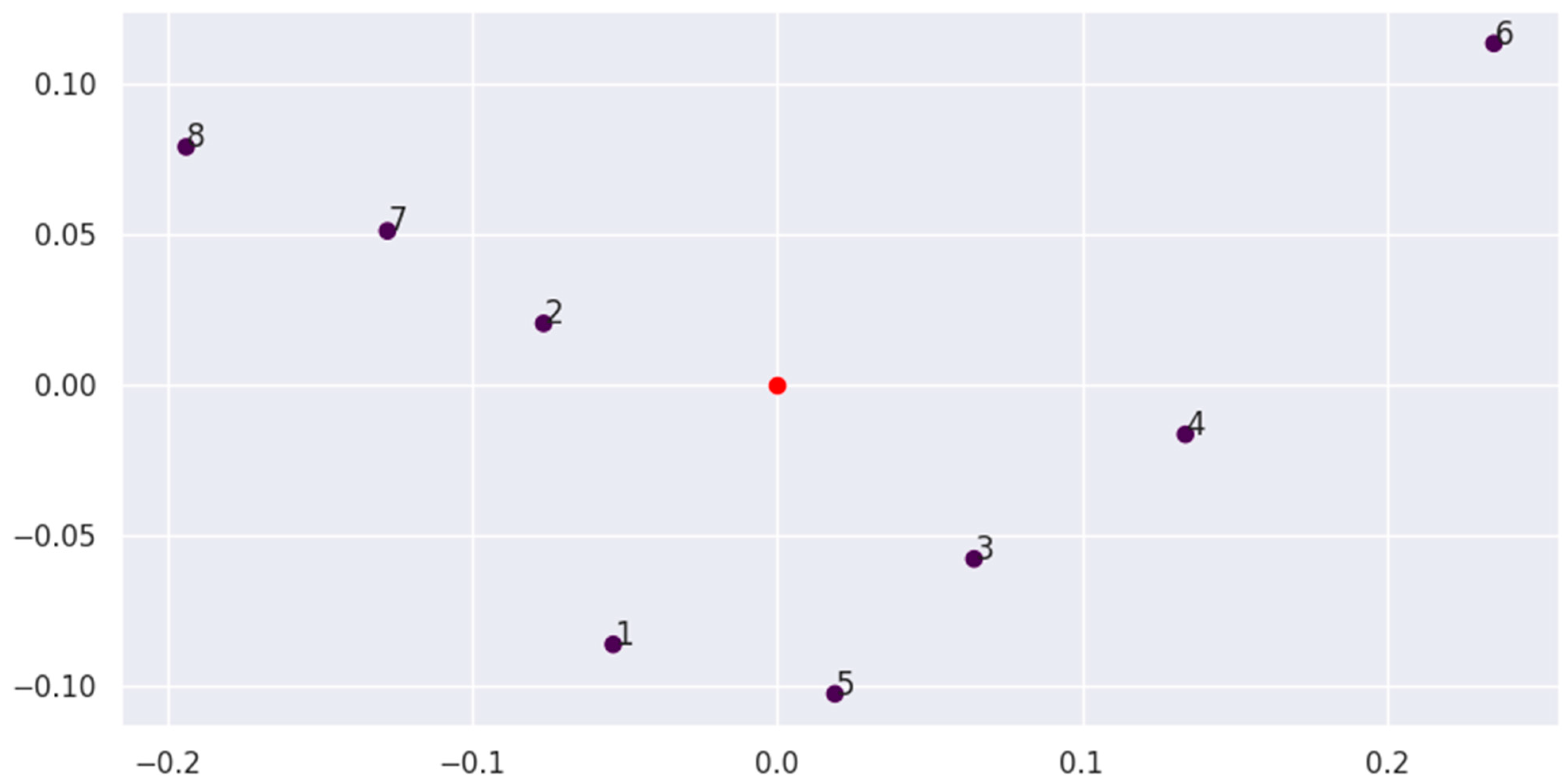
We can display the obtained results graphically by using the principal component analysis (PCA) method to reduce the m-dimensional space (where m is the number of alternatives) to a two-dimensional one. The PCA method was developed by Pearson in 1901 [41]. By reducing the space to two main components, the PCA method can convey the main behaviour, but due to data loss, there may be inaccuracies in the image. We note that Figure 1 gives only an approximate understanding of the locations of the group points, and the exact distance or criterion weight cannot be determined from the image.
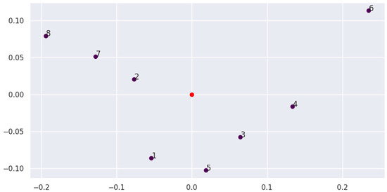
Figure 1.
Criteria weights and the centre of the criteria group in two-dimensional space.
The numbers of the points in Figure 1 correspond to the criterion numbers (Cr). The red point represents the centre of the criteria group. Figure 1 shows the distance from the centre to the points and their positions relative to each other, determining the centre of a group of criteria near a dense collection of points.
From an analysis of the graphical results, we see that the criteria are divided into the following two subgroups: the first contains Cr1 (price), Cr5 (processor sum of frequency), Cr3 (operational memory), and Cr4 (battery capacity), while the second contains Cr2 (storage), Cr7 (rear primary camera), and Cr8 (second rear camera). Criterion Cr6 (front camera) seems to be an anomaly, as it is located far from the centre and the other criteria. A semantic interpretation of the depicted points in Figure 1 indicates that the first subgroup represents technically important criteria, i.e., the basic characteristics of the phone that determine its fast operation, as well as the rather important criterion of price. The second subgroup of criteria relates to user-friendliness, document storage memory, and the quality of the primary cameras. The image quality of the front camera (Cr6) is an individual point that is of the least importance when choosing a mobile phone.
In Section 3.2, which compares objective weighing methods, the final phone selection is determined using the entropy, Centroidous, CRITIC, SD, mean, and MEREC methods.
3.1. Examination of the Stability Dependence of the Centroidous Method on the Distance Measure
If a mathematical model or method is resistant to changing its parameters, it can be used in practice [2]. Statistical modelling with a sequence of random numbers from a given distribution is used to test the model [42]. The stability of the Centroidous method is examined in this subsection in relation to the chosen distance.
Euclidean (3), which is conventionally used in the K-means clustering method, as well as Manhattan (6) and Chebyshev (7), distances are studied.
The formula for calculating the Manhattan distance is the sum of the absolute difference of the criteria vectors to the group centre of gravity , as follows:
The Chebyshev distance determines the maximum values of the vectors by calculating the absolute difference between the criteria’s vectors and the group’s centre of gravity, as follows:
The stability of the method is investigated in the following way:
Step 1. Data processing: Dataset is read. The data are normalised using Formula (1), resulting in matrix .
Step 2. Using Formula (2), the centre of gravity, , of the group of criteria is calculated.
Step 3. Distances from the group centre to each criterion are calculated. The formulas Manhattan (6), Euclidean (3), and Chebyshev (7) are used to determine the distance. The result is the following three distance vectors: , , and .
Step 4. Next, applying Formulas (4) through (5) based on the obtained distances , , and , the weights of the criterion, , are determined. The following three vectors of criteria weights are created as a result: , , and .
Step 5. The stage of creating new matrices (, ) and calculating the weights of the criteria, . The matrix numbers change slightly, increasing or decreasing by q%, thus creating a new matrix .
Using a statistical modelling technique, quasi-random numbers for matrices are produced from a uniform distribution in the interval [] for each number. The stability is checked with a equal 5% и 10%.
Step 6. The actions outlined in stages 2 through 4 are then carried out in a repeated loop (). The previously obtained weight results are combined with new ones into matrices , , and .
The matrices will have records, and the first column will have the initial weights determined from the original data. The columns will match the weights of the created matrices.
Step 7. A quality assessment of the Centroidous method using Euclidean, Manhattan, and Chebyshev distance calculations is carried out. The estimate is based on the obtained values of the weights , , and , where ; . MRE, RRM-BR, and RRM-AR metrics are used in the model’s quality assessment process.
- The mean relative error (MRE) metric indicates how the weights deviate on average from the slightly modified matrix and the primary weights . The metric is not defined at , or it may increase at very small values of the initial weights. The following formula determines the MRE:Summarising the obtained MRE results for all criteria , the mean and maximum error values are calculated.
- The rank repeatability metric (RRM) evaluates the frequency of repetition of the ranks of the weights of the criteria obtained from the initial matrix . Setting the frequency of recurrence of the best rank (RRM-BR) [2,43], which in this instance, corresponds to the greatest value of the criterion’s weight, is one of the practices. Another metric, the rank repeatability metric of all ranks (RRM-AR) [2] tracks the repetition of all the ranks. At first, the RRM is calculated for each criterion. Then they are averaged into one RRM-AR value.
The stability of the proposed Centroidous method is tested on real data that describe mobile phones (Table 1 and Table 2). The calculations of method stability testing were performed in Python (version 3.10.12) using the Google Research Collaboratory.
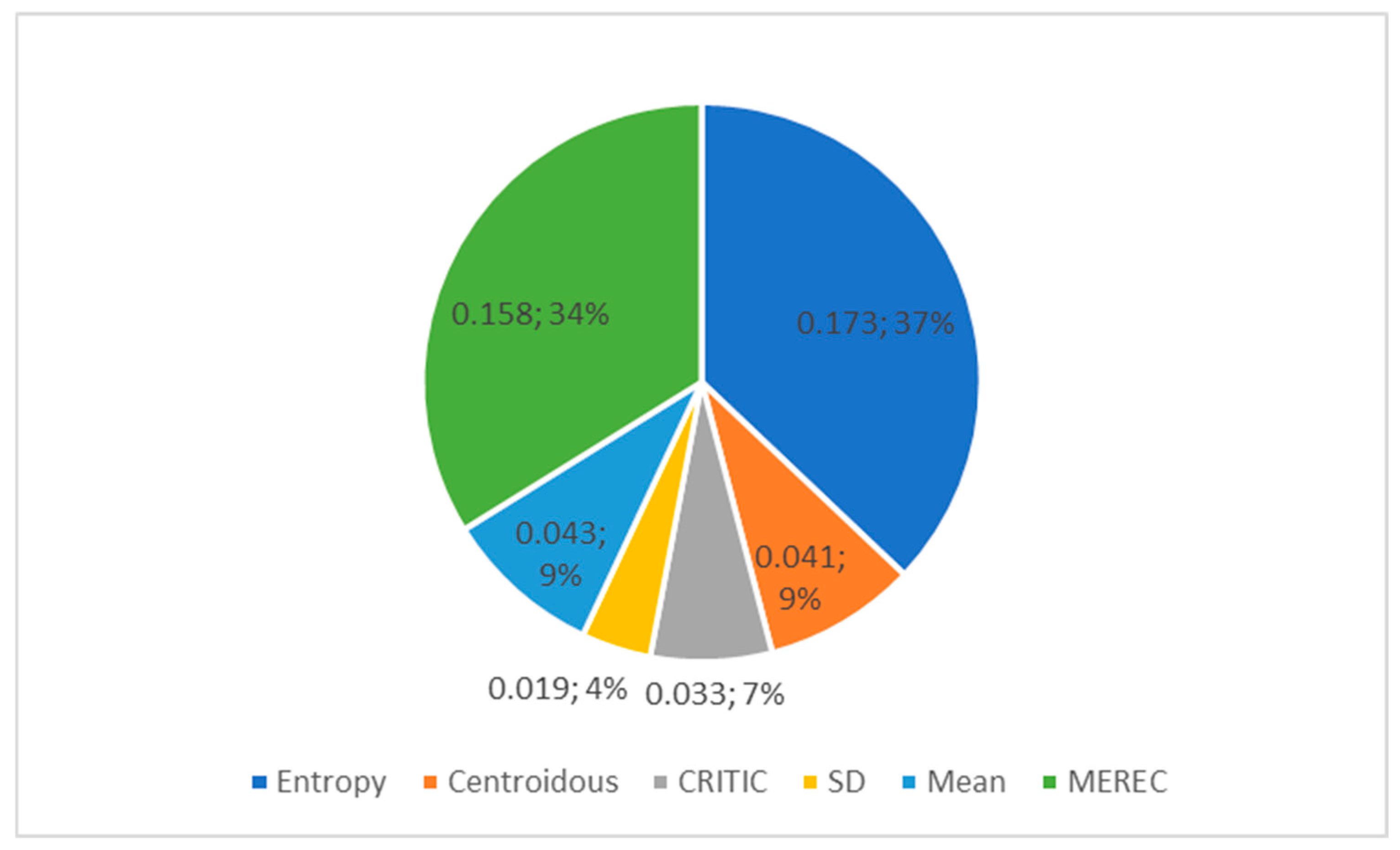
The results of the criteria , , and of weights established by the Centroidous method using Euclidean, Manhattan, and Chebyshev distances (Step 3) are presented in Table 6. The smallest value of standard deviation (based on the entire population) of criterion weights was noted in the case of the Manhattan distance—0.019. The greatest difference between the criterion weights is observed when using the Euclidean (0.04) and Chebyshev (0.053) distances.
Table 6.
Criterion weights determined using the Centroidous method applying different distance measures.
The weight of the Cr3 criterion is most significant when using the Euclidean and Manhattan distances. The ranked results of the weights for criteria Cr4 and Cr5 differ when these distances are used. Since the weights of the criteria Cr1, Cr2, Cr4, and Cr5 differ only by hundredths, it can be argued that the results for the Euclidean and Manhattan distances are very similar. In contrast, when using the Chebyshev distance, the results are significantly different; Cr3 ranks third, while Cr5 ranks first. When comparing the ranked results of the Chebyshev and Euclidean distances, the criteria Cr4 and Cr7 match.
After receiving the initial weights of the criteria (Table 6), new matrices were created in a cycle s times, changing the initial matrix by q% (steps 5 and 6). Table 7 provides the results of the mean relative error (MRE) metric for 10 repetitions of the testing of stability of the Centroidous method using the Euclidean distance, with q = 5% and s = 100. The smaller the value of the MRE, the more reliable and stable the method is. Intervals of min-max values for all ten repetitions will be indicated in the future.
Table 7.
MRE of the criteria weights, calculated using Euclidean distance, q = 5% 100 iterations, 10 repetitions.
Table 8 provides MRE intervals when checking the stability of the Centroidous method for 100 iterations (q = 5%) using Euclidean, Manhattan, and Chebyshev distances. A comparison of the mean and maximum MRE values shows that the smallest error is when using the Manhattan distance, although the difference between the former and the Euclidean is negligible. The maximum MRE values when using the Chebyshev distance are almost twice as high as those for other distance measures.
Table 8.
MRE interval of the criteria weights, q = 5% 100 iterations, 10 repetitions.
We note that with a larger number of iterations, s = 10,000 (q = 5%), the MRE error interval narrows (Table 9). The trend remained similar to Table 8. The use of the Euclidean and Manhattan distances ensures a more stable behaviour of the method. The use of the Chebyshev distance significantly increases the MRE.
Table 9.
MRE interval of the criteria weights, q = 5% 10,000 iterations, 10 repetitions.
Next, the data change interval was increased to 10% (Table 10 and Table 11). During the comparison of the mean MRE values at s = 100 and q = 10% (Table 10), with changes of 5% (Table 8), the error increased by 49–55% when using the Euclidean distance, 51–52% when using the Manhattan distance, and 51–56% when using the Chebyshev distance. A comparison of the results of Table 9 and Table 11, at s = 10,000, shows that the average MRE error values increased by 51% across all distance measures.
Table 10.
MRE interval of the criteria weights, q = 10% 100 iterations, 10 repetitions.
Table 11.
MRE interval of the criteria weights, q = 10% 10,000 iterations, 10 repetitions.
From Table 10 and Table 11, we can see the difference in using the Manhattan and Euclidean distances in the Centroidous method more clearly. As the iterations increase, the error interval narrows. The average MRE error is smaller when using the Manhattan distance; this results in a more stable behaviour of the method.
After summarising the results of stability of the Centroidous method using different values of MRE distance, it can be noted that the Chebyshev distance showed high values of errors. During the testing of stability with a 5% q interval of change, the results of errors for the Euclidean and Manhattan distances are similar. After the data change interval q is increased to 10%, the lowest MRE was observed using the Manhattan distance.
Table 12 and Table 13 use other metrics of the method’s quality. Higher values of the RRM-BR and RRM-AR metrics indicate better method stability. The RRM-BR metric records the repetition of the rank of the best criterion obtained from the initial data matrix (Table 2).
Table 12.
RRM-BR metric interval, 10 repetitions.
Table 13.
RRM-AR metric interval, 10 repetitions.
According to the RRM-BR metrics (Table 12), the method is more stable when using the Manhattan distance. A high stability rate is also observed when using the Euclidean distance, above 91%. The use of the Chebyshev distance showed poor results. The stability values of the method are higher with a smaller change in data q. As the verification iterations s increase to 10,000, the stability interval of the method changes by up to 3%.
The RRM-AR metric records the repetition of ranks of all criteria obtained from the initial data matrix. At q = 5%, the best stability result of the method is observed when using the Chebyshev distance. The stability of the Centroidous method when using the Euclidean and Manhattan distances is similar. At q = 10%, the method is more stable when using the Euclidean and Manhattan distances.
Based on the RRM-BR metric values, the Centroidous method is more stable when using the Manhattan and Euclidean distances. During the assessment of stability by repetition of all ranks of criteria (RRM-AR metric), the Chebyshev distance showed the best value at q = 5%. At q = 10%, the method is more stable when using the Euclidean and Manhattan distances.
3.2. Comparison of Centroidous with Other Methods for Calculating Objective Weights
In this study, Centroidous is compared with the following methods: entropy, criteria importance through intercriteria correlation (CRITIC), standard deviation (SD), mean, and the method based on the removal effects of criteria (MEREC).
The entropy method was proposed by Channon in 1948 within the framework of the information theory and is also used to determine objective criterion weights. The method evaluates the structure of the data array and its heterogeneity [16]. According to information theory, the lower the information entropy of a criterion, the greater the amount of information the criterion represents, i.e., the greater the weight this criterion has. For the initial data array, sum normalisation is used. This normalisation does not provide the ability to convert individual negative numbers to positive values. The use of logarithm ln in the entropy method for negative numbers and zero was not determined. Therefore, the entropy method is limited in handling negative numbers and zeros in the original dataset.
The CRITIC method determines the weights of the criteria by analysing the contrast intensity and the conflicting character of the evaluation criteria [3]. Accordingly, the standard deviation and the correlation between the criteria are calculated. The method uses min–max normalisation for the initial data array.
The SD method determines the weights of criteria based on their standard deviations [3]. In order to obtain criterion weights, the values of criteria deviations are divided by the sum of these deviations.
In this study, the mean method determines the weights of the criteria based on their mean values. In order to obtain criterion weights, the average values of the criteria are divided by the sums of these values.
The MEREC method determines the importance of a criterion by temporarily excluding it and analysing changes in the results. The criterion that has a greater impact when excluded is determined as having a greater significance. The MEREC method uses a data transformation (like the SAW method) that determines the best value to be 1. If there are negative values in the maximising criterion or there are zeros in the initial dataset, this will limit the use of the MEREC method due to the uncertain values of the logarithm ln.
In order to compare methods for the determination of objective weights, a mobile phone dataset was used (Table 1). The following criterion weight values were obtained with the use of the entropy, Centroidous, CRITIC, SD, mean, and MEREC methods (Table 14). A graphic representation of the weights is presented in Figure 2.
Table 14.
Objective weights of mobile phone criteria determined using different methods.

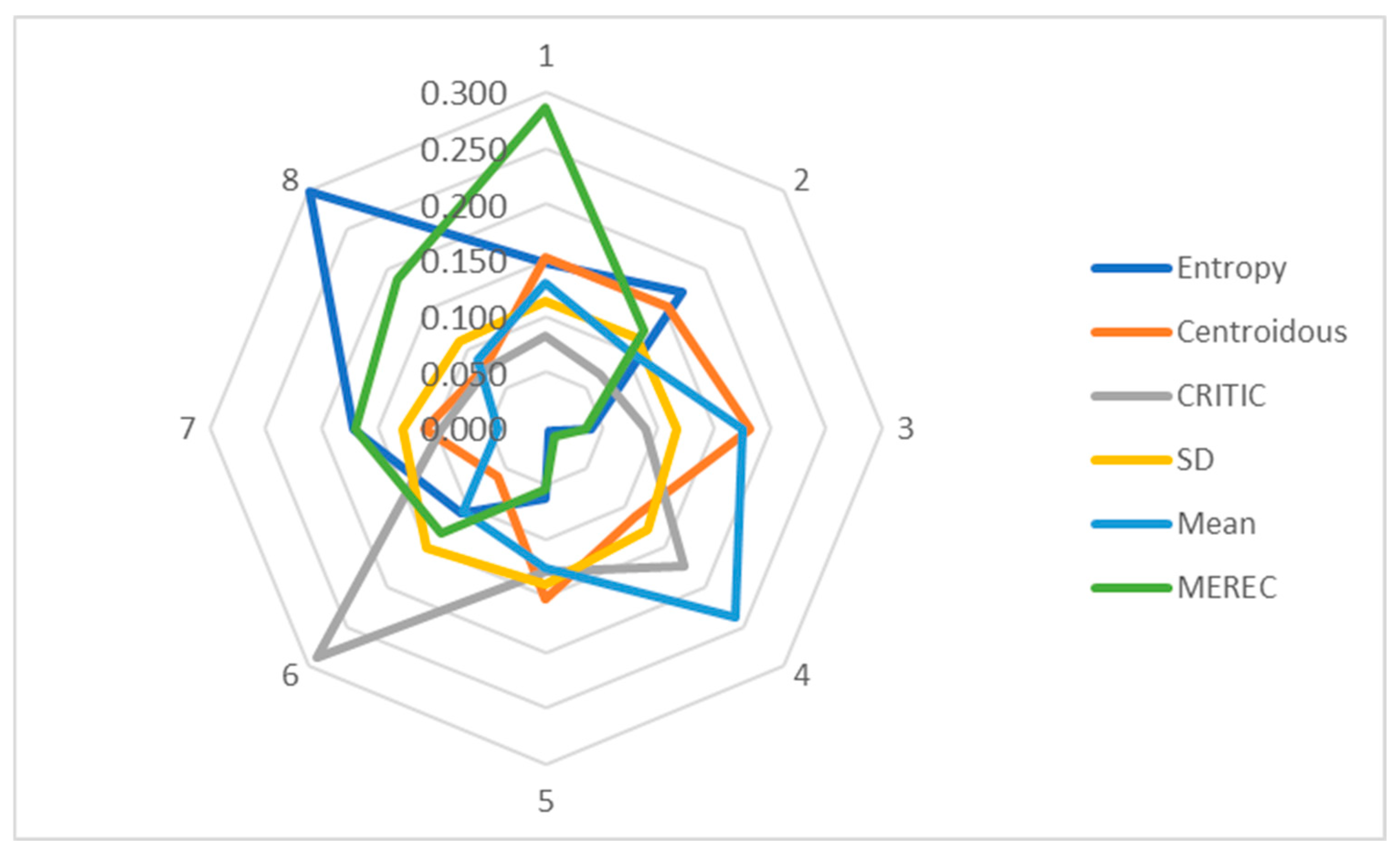
Figure 2.
Graphical representation of mobile phone criteria weights determined using different methods.
The determined weights of the criteria vary significantly (Figure 2). Entropy assigned the highest weight to the Cr8 criterion (second rear camera), and MEREC identified this criterion as the second most important. In other methods, such as Centroidous, CRITIC, and mean, this criterion turned out to be second to last in importance, and the SD method identified Cr8 as the criterion with the least weight. Centroidous gave the Cr3 criterion (operational memory) the highest weight, the mean method identified it as the second most important, and the CRITIC and SD methods identified it as the fifth most important. The CRITIC and SD methods assigned the highest weight to the Cr6 criterion (front camera). The mean method assigned the greatest weight to the Cr4 criterion (battery capacity), while MEREC assigned it the least weight. MEREC assigned the highest weight to the Cr1 criterion (price). The SD method has the same values of criterion weights (C1 and C2).
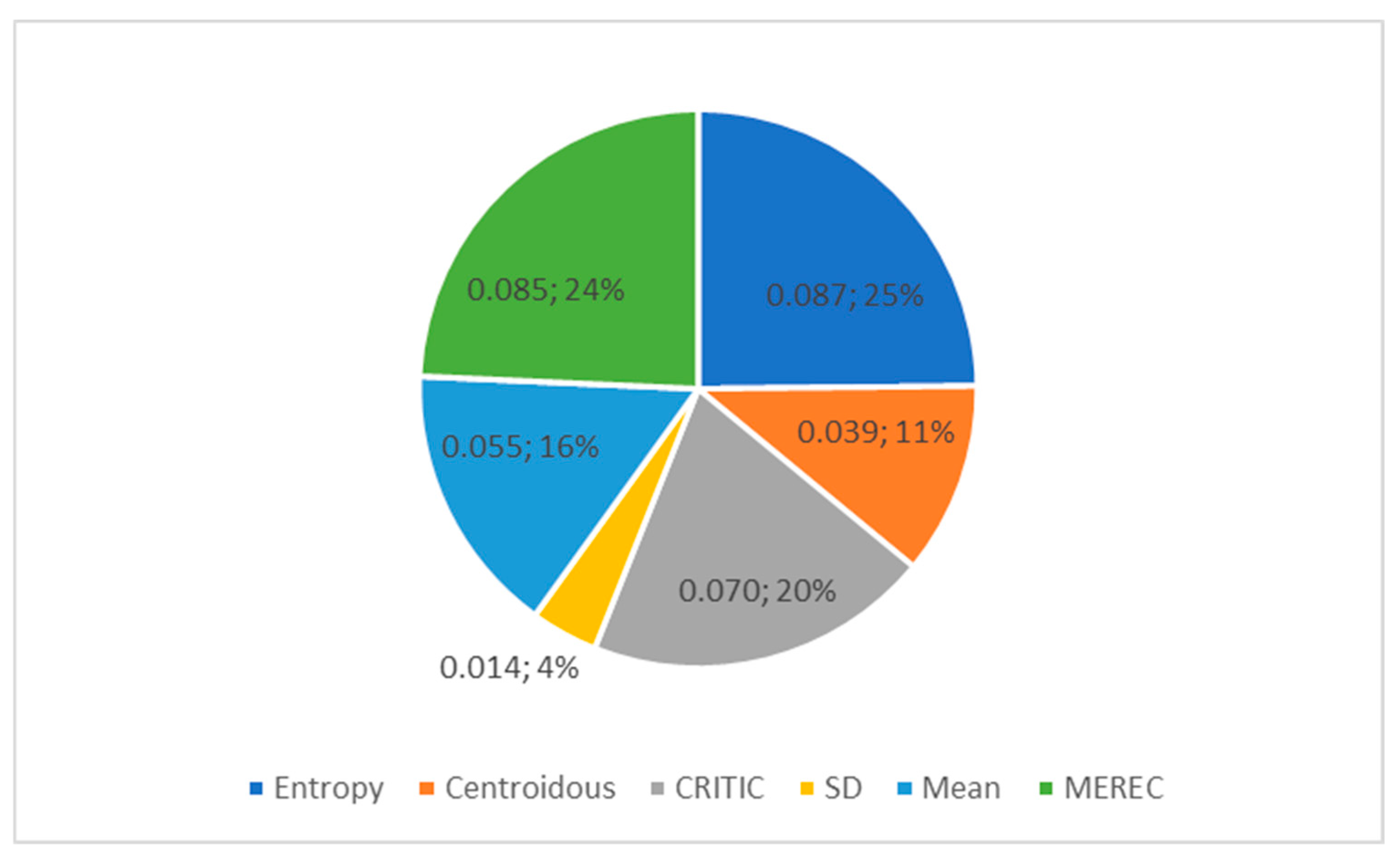
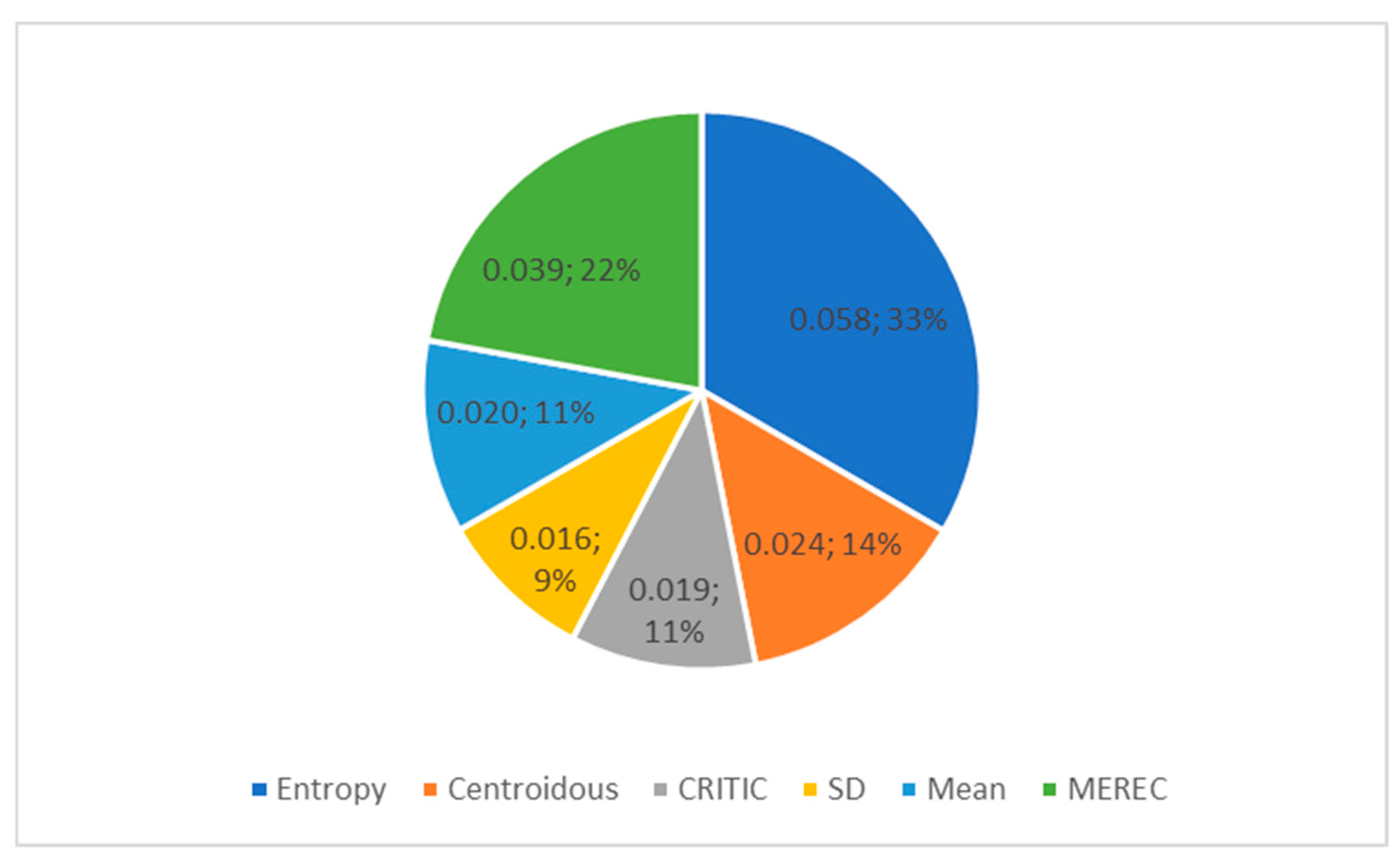
The standard deviation of criterion weights (Figure 3) shows the spread of values. The widest spread of criterion weight values is found in the entropy, CRITIC, and MEREC methods. The SD method has the smallest spread, and the weights differ little from each other (Table 14).
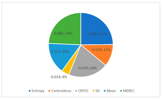
Figure 3.
Standard deviation of criteria weights from Table 14 determined using different methods.
Correlation values can indicate the similarity of the algorithms of the methods used. Table 15 shows a high correlation between the MEREC and entropy methods (0.708), as well as CRITIC and SD methods (0.879). There is also a weak correlation of 0.29 between the mean and Centroidous methods.
Table 15.
Correlation of weights of mobile phone criteria determined using different methods.
Next, the weights of the criteria (Table 14) were used to determine the best alternative, i.e., a mobile phone, by calculating with the use of the simple additive weighting (SAW) [10] method. The values of the SAW method are presented in Table 16, the ranked results of the evaluations are in Table 17.
Table 16.
Estimates of mobile phones, using SAW method.
Table 17.
Ranked values of alternative estimates determined using the SAW method.
The best alternative, A1, is clearly determined using the weights obtained by all methods for the determination of objective weights (Table 17). This was due to the fact that the maximising criteria evaluations of alternative A1 itself dominate over other alternatives. The entropy, CRITIC, SD, and mean methods placed the A5 alternative in second place. The ranked results of the Centroidous method are similar to those of the mean method.
In this example, each method showed its uniqueness. The ranked results completely matched only for the CRITIC and SD methods, the weights of which showed a high correlation.
Three sets of data were artificially generated (Table 18) for a more thorough study of the behaviour of the methods. They reflect different problematic issues identified during data analysis. A linear relationship and high correlation were identified among criteria C1, C2, C3, and C4 (Table 19) in the first generated dataset (Table 18).
Table 18.
Artificially generated data-1 with high correlation between criteria.
Table 19.
Correlation between data criteria in data-1.
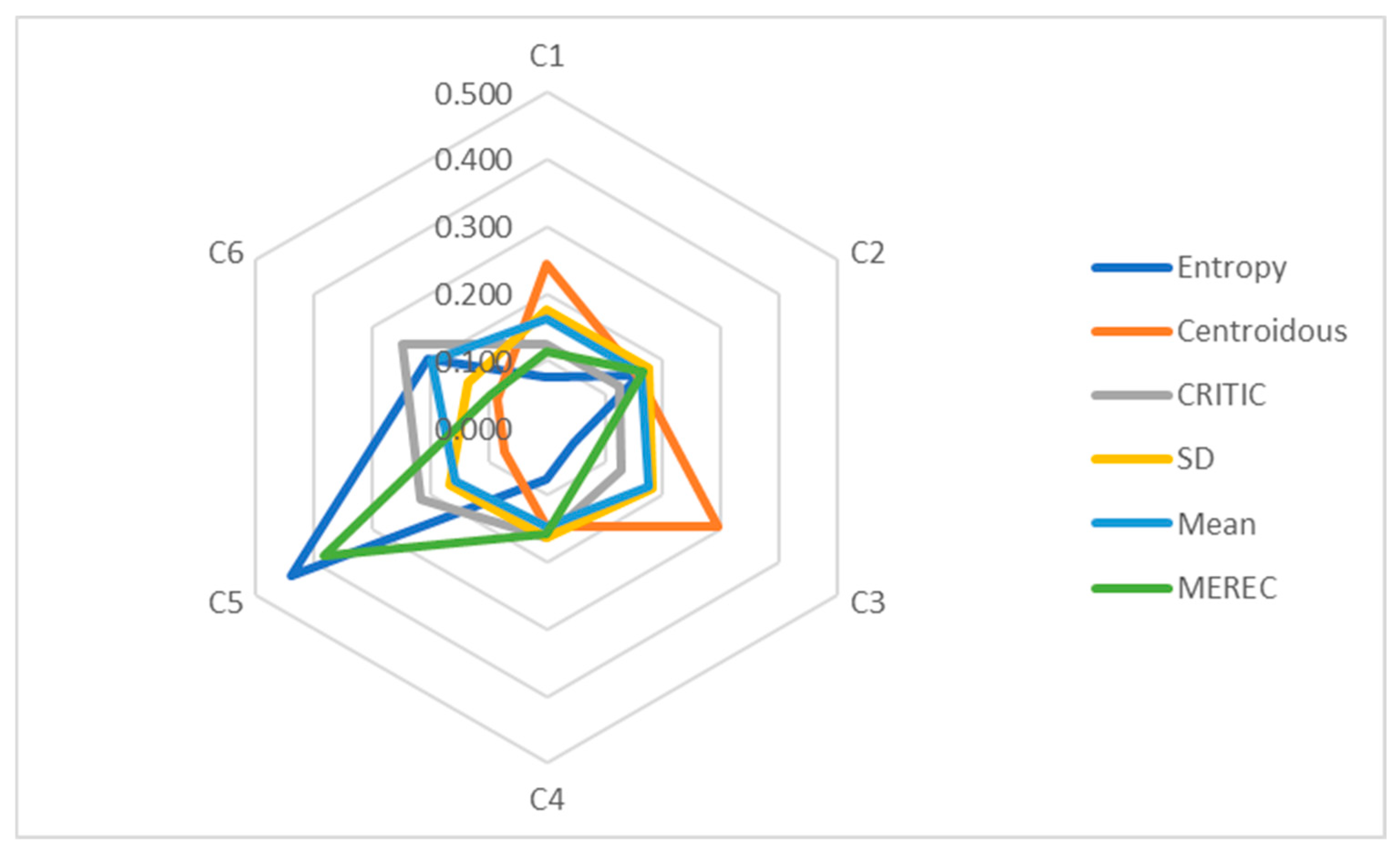
Next, the weights of the criteria are established (Table 20) using the entropy, Centroidous, CRITIC, SD, mean, and MEREC methods with the use of artificially generated data-1. The entropy and MEREC methods assign the highest weight to criterion C5, the Centroidous and SD methods assign the highest weight to criterion C3, and the CRITIC and mean assign the highest weight to criterion C6 (Figure 4). All criterion weights are clearly defined; there are no zero-weight criteria.
Table 20.
Objective weights of data-1 criteria determined using different methods.
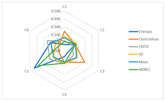
Figure 4.
Graphical representation of data-1 criteria weights determined using different methods.
In order to trace the dependence of all weights of the criteria, we will analyse the correlation of the weights presented in Table 21. A high correlation was found between the results of the entropy and MEREC methods—0.894. The average correlation was between entropy and CRITIC (0.656), Centroidous and SD (0.687), and CRITIC and mean (0.503).
Table 21.
Correlation of weights of data-1 criteria determined using different methods.
The entropy, MEREC, and Centroidous methods had the largest standard deviation of criterion weights. The mean and SD methods had the smallest deviation between the weights (Figure 5).
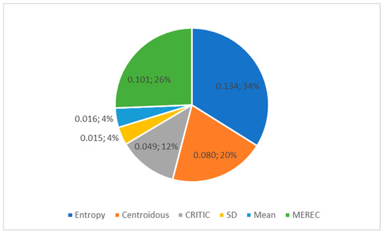
Figure 5.
Standard deviation of criteria weights from Table 20 determined using different methods.
The second artificially generated dataset, data-2, has slight differences in the means of the alternatives (Table 22). The maximum difference between the means of the alternatives is 1.43.
Table 22.
Artificially generated data-2 with a slight difference between mean values.
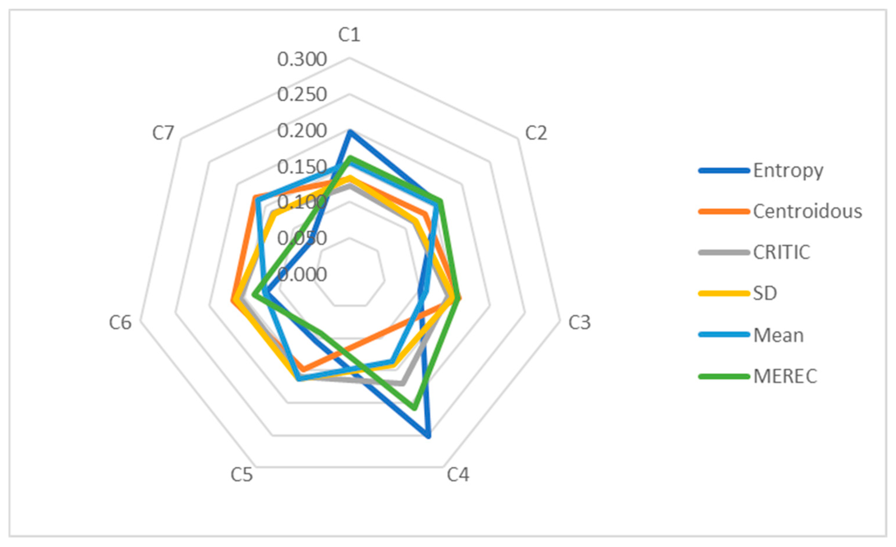
Table 23 shows the weights of the criteria established using the entropy, Centroidous, CRITIC, SD, mean, and MEREC methods using data array-2. The highest weight was assigned to criterion C3 using the entropy, CRITIC, and MEREC methods, and the Centroidous and mean methods assigned the highest weight to criterion C7. The mean and SD methods have the same criterion values (C1 and C2, C5 and C6).
Table 23.
Objective weights of data-2 criteria determined using different methods.
Figure 6 clearly shows the dominance of criterion C4. The entropy and MEREC methods indicate this more accurately. The remaining criterion values are less prominent.
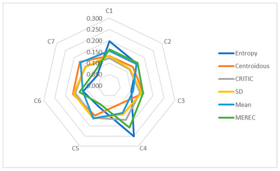
Figure 6.
Graphical representation of data-2 criteria weights determined using different methods.
There is a strong correlation between the values of the criteria of the entropy and MEREC methods—0.871—and the CRITIC and SD methods—0.748. The correlation of the results between the Centroidous and SD methods is average (0.35), and the correlation between the CRITIC and entropy methods is weak (0.146) (see Table 24).
Table 24.
Correlation of weights of data-2 criteria determined using different methods.
A high value of the standard deviation of criterion weights is observed in the entropy, MEREC, and Centroidous methods (Figure 7). These methods clearly define the weights of the criteria. The weights obtained using the SD method differ little from each other.

Figure 7.
Standard deviation of criteria weights from Table 23 determined using different methods.
The third artificially generated data array, data-3, has large differences in the means of the alternatives (Table 25). The maximum difference between the means of the alternatives is 672.43.
Table 25.
Artificially generated data-3 with large differences in mean values.
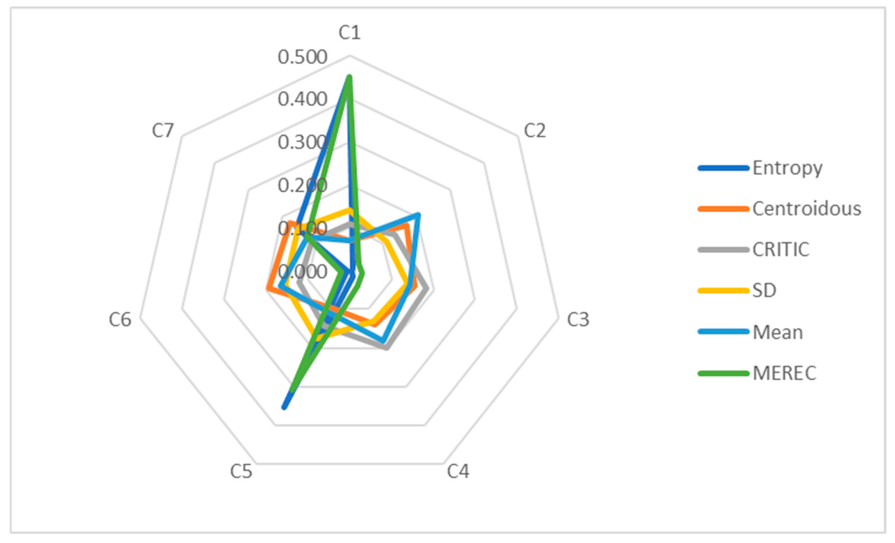
Table 26 shows the weights of the criteria established using the entropy, Centroidous, CRITIC, SD, mean, and MEREC methods using the data-3 array. The greatest weight is assigned to the C1 criterion by the entropy and MEREC methods. The other methods determined the greatest weight based on different criteria, as follows: Centroidous—C6, CRITIC—C4, SD—C5, mean—C2. All weights are defined precisely; there is no repetition of the values of the weights of criteria.
Table 26.
Objective weights of data-3 criteria determined using different methods.
C1 and C5 criteria, determined using the entropy and MEREC methods, stand out in Figure 8. The outline of the mean method is noticeable, as well. A large standard deviation is observed in the entropy and MEREC methods (Figure 9). The other methods distributed the importance between the criteria fairly evenly when a difference in the means of the initial data (Table 25) was large and differences in the standard deviations were not large (Figure 9).

Figure 8.
Graphical representation of data-3 criteria weights determined using different methods.

Figure 9.
Standard deviation of criteria weights from Table 26 determined using different methods.
The analysis of correlations of weights for all criteria showed a strong dependence between the entropy and MEREC methods (0.992) and the Centroidous and mean methods (0.731). The average correlation was identified between the CRITIC and mean methods (0.438) and the SD and MEREC methods (0.399) (see Table 27).
Table 27.
Correlation of weights of data-3 criteria determined using different methods.
The entropy, Centroidous, CRITIC, SD, mean, and MEREC methods have shown their uniqueness when determining the criterion weights. Criterion weights are clearly identified in all datasets. A high correlation between the results of the entropy and MEREC methods (0.71, 0.84, 0.87, 0.99) was revealed in all examples. A high correlation was also observed for the CRITIC and SD methods (0.88, 0.75), and an average correlation was observed for the entropy and CRITIC methods (0.66, 0.15), CRITIC and mean methods (0.44), entropy and SD methods (0.5, 0.48), and SD and MEREC methods (0.4). There were high and average correlations between the results of the Centroidous and mean methods (0.731, 0.29) and the Centroidous and SD methods (0.69, 0.35).
The largest deviations in criterion weights are observed in the entropy, MEREC, Centroidous, and CRITIC methods. Weights with the same values may appear in the mean and SD methods in cases in which the average values of the initial data alternatives differ little from each other.
4. Discussion and Conclusions
At the time of use, statistical data from the Web of Science database indicated that the objective weighting method is the most widely applicable in the context of clinical trials. An analysis of previous research papers dedicated to methods of determining objective weights shows that in most cases, these algorithms calculate statistical indicators, such as the correlation (CRITIC, D-CRITIC, CCSD, CRITIC-M, ROCOSD, EWM-CORR), standard deviation (CCSD, CRITIC-M, SECA, ROCOSD), entropy (entropy, EWM-CORR, IDOCRIW), or logarithmic exponent (MEREC, LOPCOW).
The Centroidous method presented in this study represents a new perspective in the area of MCDM approaches. Centroidous is theoretically substantiated and relies on the concept of centroid clustering. Clustering methods are well-known in machine learning as a group of unsupervised learning methods. It is assumed that each cluster consists of a set of values that are fairly well approximated by the cluster centre [44]. When determining the weights of the criteria, the distance from the criterion to the centre of the cluster is taken into consideration; criteria located near the centre of the group are interpreted as more important, and the most distant criteria of the group have the smallest weights. In a broader context, “single” objects located far from the centre are perceived as outliers.
A literature analysis confirmed the mathematical justification of the Centroidous method proposed in this paper. The idea that the core elements, which are the most important in the context of a given group of criteria, accumulate in the centre of the criteria group resonates with the mathematical justification of other methods. Vaghefi claims that WLR typically uses the reciprocal of the diagonal element of the error covariance matrix [39]. It follows that the smaller the error variance, the more weight an observation receives. In the case of the Centroidous method, greater weight is determined for objects that are closer to the centre of the group. The centre of the group itself is defined as closer to a denser cluster of points, the dispersion of which is smaller. The logic of the Centroidous method, assuming that the weight of a criterion is inversely proportional to the distance of this criterion to the centre of the group, is also confirmed in the WKNN and IDW methods.
The use of distance is common in various areas of machine learning, including regression, classification and clustering. Distance is a basic concept in the fundamental sciences that allows us to determine the degree of similarity or difference between objects. Elen and Avuçlu argue that Euclidean distance is the most favoured distance measure in practice [22]. Based on the literature reviewed, the Centroidous method proposed to use Euclidean distance as the preferred measure.
In this study, a demonstration of the application of the new Centroidous method has been presented based on an example in which eight criteria for choosing a mobile phone were assessed. We note the ease of implementation of the Centroidous method and the possibility of the semantic interpretation of the results. The proposed Centroidous method can be used to calculate objective criteria weights based on a previously defined system of criteria.
In this research, the use of different distance measures in the Centroidous method was examined more thoroughly. For this purpose, the stability of the Centroidous method was tested using the following distance measures: Euclidean, Manhattan, and Chebyshev. A comparison of distance measures was examined on a real mobile phone dataset collected by the author of the paper.
Using the Manhattan distance, the obtained values of the criteria weights were found to be very similar; the standard deviation of the values was 0.019. In the case of using Euclidean and Chebyshev distances, the weights are determined more precisely; there are no equal criteria weights.
The method stability verification indicated Manhattan and Euclidean distances as more preferred measures to be used in the Centroidous method. The RRM-AR metric at q = 10% and s = 10,000 showed 58.59% to 59.11% stability using Euclidean distance and 58.87% to 59.27% using Manhattan distance. According to RRM-BR metric values using Manhattan distance (when q = 5%, s = 10,000), the stability of the Centroidous method is 100%, while using Euclidean distance, the stability is 95.71–96.38%. Comparing the mean and maximum MRE values, the smallest error occurs using the Manhattan distance, although the difference between that and Euclidean is not significant. As the number of iterations increases, the MRE error interval narrows, meaning that the values of the metric are almost unchanged when rechecked.
This paper provides a comprehensive comparison of the Centroidous method with established objective weighting methods entropy, CRITIC, SD, mean, and MEREC. The comparative analysis is performed on a real mobile phone dataset. With the weights obtained from all the methods used in the comparative analysis, the alternatives were evaluated using the SAW method. The determination of the second (rank 2) best alternative A5 coincided with the entropy, CRITIC, SD, and mean methods. The Centroidous method A5 alternative ranked third.
In order to scrutinise the entropy, Centroidous, CRITIC, SD, mean, and MEREC methods, three datasets were artificially generated, which reflect different problematic points detectable in the data analysis. The first generated dataset shows a linear relationship of the four criteria, and data-2 has slight differences in the mean values of the alternatives, the maximum difference of which is 1.43. The third artificially generated dataset, data-3, has large differences in the mean values of the alternatives, the maximum difference between which is 672.43.
The criteria weights were clearly determined using the entropy, Centroidous, CRITIC, SD, mean, and MEREC methods on all datasets. The methods showed their uniqueness in determining the criterion weights; the results of the weights did not have many coincidences. However, a high correlation between the entropy and MEREC methods was found across all datasets (0.71–0.99).
Also, the correlation of the criteria weights set by CRITIC and SD methods (0.88, 0.75) on mobile phones and data-2 datasets should be noted. The Centroidous method results correlate with the determined weights of the mean method on the data-3 dataset (0.73) and the SD method (0.69) on the data-1 dataset.
The entropy, MEREC, Centroidous, and CRITIC methods have the highest standard deviation of the criterion weights. In the mean and SD methods, the weights have small deviations, and this may result in weights with the same values when the mean values of the original data of the alternatives differ slightly.
In previous studies, the author of this article analysed and compared methods for determining subjective weights for AHP and FAHP [42], as well as a number of FAHP methods [2] involving stability calculations. Hence, one area for further research will be a comparative analysis of methods for determining objective weights using a stability verification algorithm, including the Centroidous method. Another area for further research is the division of one large group of criteria into subgroups using clustering methods. In general, criteria are broken down into subgroups by experts, according to their semantic interpretation. It is assumed that the automatic division of criteria into subgroups based on the distance between the criteria or the density can provide helpful information for a more accurate determination of the criteria weights.
Funding
This research received no external funding.
Data Availability Statement
The original contributions presented in the study are included in the article, further inquiries can be directed to the corresponding author.
Conflicts of Interest
The author declares no conflict of interest.
References
- Web of Science. Clarivate. Available online: https://webofscience.clarivate.cn/wos/woscc/basic-search (accessed on 28 May 2024).
- Vinogradova-Zinkevič, I. Comparative sensitivity analysis of some fuzzy AHP methods. Mathematics 2023, 11, 4984. [Google Scholar] [CrossRef]
- Diakoulaki, D.; Mavrotas, G.; Papayannakis, L. Determining objective weights in multiple criteria problems: The CRITIC method. Comput. Oper. Res. 1995, 22, 763–770. [Google Scholar] [CrossRef]
- Pala, O. A new objective weighting method based on robustness of ranking with standard deviation and correlation: The ROCOSD method. Inf. Sci. 2023, 636, 118930. [Google Scholar] [CrossRef]
- Krishnan, A.R.; Kasim, M.M.; Hamid, R.; Ghazali, M.F. A modified CRITIC method to estimate the objective weights of decision criteria. Symmetry 2021, 13, 973–992. [Google Scholar] [CrossRef]
- Wang, Y.M.; Luo, Y. Integration of correlations with standard deviations for determining attribute weights in multiple attribute decision making. Math. Comput. Model. 2010, 51, 1–12. [Google Scholar] [CrossRef]
- Žižović, M.; Miljković, B.; Marinković, D. Objective methods for determining criteria weight coefficients: A modification of the CRITIC method. Decis. Mak. Appl. Manag. Eng. 2020, 3, 149–161. [Google Scholar] [CrossRef]
- Keshavarz-Ghorabaee, M.; Amiri, M.; Zavadskas, E.K.; Turskis, Z.; Antucheviciene, J. Simultaneous evaluation of criteria and alternatives (SECA) for multi-criteria decision-making. Informatica 2018, 29, 265–280. [Google Scholar] [CrossRef]
- Liu, S.; Chan, F.T.S.; Ran, W. Decision making for the selection of cloud vendor: An improved approach under group decision-making with integrated weights and objective/subjective attributes. Expert Syst. Appl. 2016, 55, 37–47. [Google Scholar] [CrossRef]
- Hwang, C.L.; Yoon, K. Methods for multiple attribute decision making. In Multiple Attribute Decision Making; Springer: Berlin/Heidelberg, Germany, 1981; pp. 58–191. [Google Scholar]
- Wu, R.M.X.; Zhang, Z.; Yan, W.; Fan, J.; Gou, J.; Liu, B.; Gide, E.; Soar, J.; Shen, B.; Fazal-e-Hasan, S.; et al. A comparative analysis of the principal component analysis and entropy weight methods to establish the indexing measurement. PLoS ONE 2022, 17, e0262261. [Google Scholar] [CrossRef] [PubMed]
- Podvezko, V.; Zavadskas, E.K.; Podviezko, A. An extension of the new objective weight assessment methods CILOS and IDOCRIW to fuzzy MCDM. Econ. Comput. Econ. Cybern. Stud. Res. 2020, 2, 59–75. [Google Scholar] [CrossRef]
- Mukhametzyanov, I. Specific character of objective methods for determining weights of criteria in MCDM problems: Entropy, CRITIC and SD. Decis. Making Appl. Manage. Eng. 2021, 4, 76–105. [Google Scholar] [CrossRef]
- Keshavarz-Ghorabaee, M.; Amiri, M.; Zavadskas, E.K.; Turskis, Z.; Antucheviciene, J. Determination of objective weights using a new method based on the removal effects of criteria (MEREC). Symmetry 2021, 13, 525–545. [Google Scholar] [CrossRef]
- Ecer, F.; Pamucar, D. A novel LOPCOW-DOBI multi-criteria sustainability performance assessment methodology: An application in developing country banking sector. Omega 2022, 112, 102690. [Google Scholar] [CrossRef]
- Zavadskas, E.K.; Podvezko, V. Integrated determination of objective criteria weights in MCDM. Int. J. Inf. Technol. Decis. Mak. 2016, 15, 267–283. [Google Scholar] [CrossRef]
- Odu, G.O. Weighting methods for multi-criteria decision making technique. J. Appl. Sci. Environ. Manag. 2019, 23, 1449–1457. [Google Scholar] [CrossRef]
- Vinogradova, I.; Podvezko, V.; Zavadskas, E.K. The recalculation of the weights of criteria in MCDM methods using the Bayes approach. Symmetry 2018, 10, 205. [Google Scholar] [CrossRef]
- Vinogradova-Zinkevič, I. Application of Bayesian approach to reduce the uncertainty in expert judgments by using a posteriori mean function. Mathematics 2021, 9, 2455. [Google Scholar] [CrossRef]
- Jahan, A.; Mustapha, F.; Sapuan, S.M.; Ismail, M.Y.; Bahraminasab, M. A framework for weighting of criteria in ranking stage of material selection process. Int. J. Adv. Manuf. Technol. 2012, 58, 411–420. [Google Scholar] [CrossRef]
- Yazdani, M.; Zaraté, P.; Zavadskas, E.K.; Turskis, Z. A combined compromise solution (CoCoSo) method for multi-criteria decision-making problems. Manag. Decis. 2019, 57, 2501–2519. [Google Scholar] [CrossRef]
- Elen, A.; Avuçlu, E. Standardized Variable Distances: A distance-based machine learning method. Appl. Soft Comput. 2021, 98, 106855. [Google Scholar] [CrossRef]
- Bigi, B. Using Kullback-Leibler Distance for Text Categorization. ECIR 2003. Lecture Notes in Computer Science. In Advances in Information Retrieval; Sebastiani, F., Ed.; Springer: Berlin/Heidelberg, Germany, 2003; Volume 2633. [Google Scholar] [CrossRef]
- Zhang, F.; O’Donnell, L.J. Support vector regression. In Machine Learning; Mechelli, A., Vieira, S., Eds.; Academic Press: Cambridge, MA, USA, 2020; Chapter 7; pp. 123–140. [Google Scholar] [CrossRef]
- Lee, L.H.; Wan, C.H.; Rajkumar, R.; Isa, D. An enhanced Support Vector Machine classification framework by using Euclidean distance function for text document categorization. Appl. Intell. 2012, 37, 80–99. [Google Scholar] [CrossRef]
- Zhang, H.; Liu, Y.; Lei, H. Localization from Incomplete Euclidean Distance Matrix: Performance Analysis for the SVD–MDS Approach. IEEE Trans. Signal Process. 2019, 67, 2196–2209. [Google Scholar] [CrossRef]
- Zhang, X.; Lu, W.; Pan, Y.; Wu, H.; Wang, R.; Yu, R. Empirical study on tangent loss function for classification with deep neural networks. Comput. Electr. Eng. 2021, 90, 107000. [Google Scholar] [CrossRef]
- Torres-Huitzil, C.; Girau, B. Fault and Error Tolerance in Neural Networks: A Review. IEEE Access 2017, 5, 17322–17341. [Google Scholar] [CrossRef]
- Sharma, S.; Rana, V.; Malhotra, M. Automatic recommendation system based on hybrid filtering algorithm. Educ. Inf. Technol. 2022, 27, 1523–1538. [Google Scholar] [CrossRef]
- Frahling, G.; Sohler, C. A fast K-means implementation using coresets. Int. J. Comput. Geom. Appl. 2008, 18, 605–625. [Google Scholar] [CrossRef]
- Erisoglu, M.; Calis, N.; Sakallioglu, S. A new algorithm for initial cluster centers in K-means algorithm. Pattern Recognit. Lett. 2011, 32, 1701–1705. [Google Scholar] [CrossRef]
- MacQueen, J. Some methods for classification and analysis of multivariate observations. In Proceedings of the Berkley Symposium on Mathematical Statistics and Probability; Le Cam, L.M., Neyman, J., Eds.; University of California Press: Berkeley, CA, USA, 1967; Volume 1, pp. 281–297. [Google Scholar]
- Barakbah, A.R.; Kiyoki, Y. A pillar algorithm for K-means optimization by distance maximization for initial centroid designation. In Proceedings of the IEEE Symposium on Computational Intelligence and Data Mining, Nashville, TN, USA, 30 March–2 April 2009; pp. 61–68. [Google Scholar] [CrossRef]
- Saputra, D.M.; Saputra, D. Effect of Distance Metrics in Determining K-Value in K-Means Clustering Using Elbow and Silhouette Method. In Proceedings of the Sriwijaya International Conference on Information Technology and Its Applications (SICONIAN 2019), Palembang, Indonesia, 16 November 2019; Atlantis Press: Amsterdam, The Netherlands, 2020; pp. 341–346. [Google Scholar] [CrossRef]
- Dudani, S. The Distance Weighted k-Nearest-Neighbor Rule. IEEE Trans. Syst. Man Cybern. 1975, 6, 325–327. [Google Scholar] [CrossRef]
- Gou, J.; Du, L.; Zhang, Y.; Xiong, T. A New Distance-weighted k-nearest Neighbor Classifier. J. Inf. Comput. Sci. 2012, 9, 1429–1436. [Google Scholar]
- Lu, G.Y.; Wong, D.W. An adaptive inverse-distance weighting spatial interpolation technique. Comput. Geosci. 2008, 34, 1044–1055. [Google Scholar] [CrossRef]
- Kay, S. Fundamentals of Statistical Processing, Volume I: Estimation Theory; Prentice Hall PTR: Hoboken, NJ, USA, 1993. [Google Scholar]
- Vaghefi, R. Weighted Linear Regression. Towards Data Science. 4 February 2021. Available online: https://towardsdatascience.com/weighted-linear-regression-2ef23b12a6d7 (accessed on 4 July 2024).
- Mobile Telephones. Available online: https://tele2.lt/privatiems/mobilieji-telefonai (accessed on 8 April 2024).
- Pearson, K. On lines and planes of closest fit to systems of points in space. Philos. Mag. 1901, 2, 559–572. [Google Scholar] [CrossRef]
- Vinogradova-Zinkevič, I.; Podvezko, V.; Zavadskas, E.K. Comparative assessment of the stability of AHP and FAHP methods. Symmetry 2021, 13, 479. [Google Scholar] [CrossRef]
- Vinogradova, I. Multi-Attribute Decision-Making Methods as a Part of Mathematical Optimization. Mathematics 2019, 7, 915. [Google Scholar] [CrossRef]
- Ding, H.; Huang, R.; Liu, K.; Yu, H.; Wang, Z. Randomized greedy algorithms and composable coreset for k-center clustering with outliers. arXiv 2023, arXiv:2301.02814. [Google Scholar] [CrossRef]

Disclaimer/Publisher’s Note: The statements, opinions and data contained in all publications are solely those of the individual author(s) and contributor(s) and not of MDPI and/or the editor(s). MDPI and/or the editor(s) disclaim responsibility for any injury to people or property resulting from any ideas, methods, instructions or products referred to in the content. |
© 2024 by the author. Licensee MDPI, Basel, Switzerland. This article is an open access article distributed under the terms and conditions of the Creative Commons Attribution (CC BY) license (https://creativecommons.org/licenses/by/4.0/).