Abstract
Feature selection is a basic and important step in real applications, such as face recognition and image segmentation. In this paper, we propose a new weakly supervised multi-view feature selection method by utilizing pairwise constraints, i.e., the pairwise constraint-guided multi-view feature selection (PCFS for short) method. In this method, linear projections of all views and a consistent similarity graph with pairwise constraints are jointly optimized to learning discriminative projections. Meanwhile, the -norm-based row sparsity constraint is imposed on the concatenation of projections for discriminative feature selection. Then, an iterative algorithm with theoretically guaranteed convergence is developed for the optimization of PCFS. The performance of the proposed PCFS method was evaluated by comprehensive experiments on six benchmark datasets and applications on cancer clustering. The experimental results demonstrate that PCFS exhibited competitive performance in feature selection in comparison with related models.
Keywords:
multi-view feature selection; pairwise constraints; weakly supervised learning; joint subspace; similarity learning MSC:
6208
1. Introduction
The development of data acquisition techniques and the diversification of data-processing methods make multi-view data a typical form of big data. Concretely, multi-view data is a general term for data with multiple feature representations of the same object. For example, cancers can be studied in terms of RNA gene expression, mitochondrial DNA, microRNA expression, and reverse phase protein array expression [1], where each kind of expression corresponds to a view in multi-view data. For another example, different visual descriptors, such as LBP [2], HOG [3], and SIFT [4] can be extracted from images, and each visual descriptor forms a view. For multi-view data, since views are the descriptions of the same object from different aspects, each view not only contains somewhat consistent information with the others but also contains some information complementary to the other views. How to make full use of the consistent and complementary information from multiple views to improve the data analysis performance gives rise to the flourishment of multi-view learning.
The studies on multi-view learning were conducted from various aspects, such as subspace learning [5], feature selection [6], classification [7], clustering [8], and multi-label learning [9]. More details can be found in surveys [10,11]. Among these studies, multi-view feature selection, as an important preprocessing step for dealing with multi-view high-dimensional data, has attracted extensive attention. Multi-view feature selection aims to select the most relevant features or variables for the subsequent learning tasks. Compared with multi-view subspace learning, which is an another typical way to handle the curse of dimensionality, multi-view feature selection keeps the original semantics of the variables and has an advantage in interpretability. In this paper, we focus on multi-view feature selection.
Conventionally, according to the labelling condition of the training data, multi-view feature selection methods can be grouped into three categories. That is, if the training samples are all labelled, partly labelled or all unlabeled, then the corresponding methods are categorized as supervised [12], semi-supervised [13], or unsupervised [14]. It is known that labelling samples is considerably expensive. Thus, unsupervised multi-view feature selection is more preferred in real applications. Existing unsupervised multi-view feature selection works can be divided into two groups, i.e., serial models and parallel models [15]. In the early period, serial models first concatenate all views into a big one, and then apply single-view feature selection methods on the concatenated features, such as spectral feature selection (SPEC) [16], minimum redundancy spectral feature selection (MRSF) [17], and URAFS [18]. However, approaches of this kind are not able to make full use of the consistency and complementarity between views. To overcome this deficiency, adaptive multi-view feature selection (AMFS) combines the graph Laplacian from all views [19], and Feng et al. added a multi-view manifold regularization term into the subspace learning scheme with sparsity induced by the -norm [20]. Along this line of research, Dong et al. proposed to learn consensus similarity from initial view-specific graphs, together with the sparse projection [21]. By contrast, parallel models conduct sparse projection learning on each view and merge the selected features from all views. Representative methods include MVUFS [22], RMVFS [23], ASVW [24], and JMVFG [25]. MVUFS learns pseudo-labels with local manifold regularization and simultaneously selects discriminative features from each view via sparse projection to the pseudo-label-indicating matrix [22]. RMVFS realizes view-specific sparse feature selection based on the multi-view K-means model [23]. ASVW encodes -norm sparse regularized projection learning on each view into the consensus similarity learning scheme [24]. In view of the effectiveness of these methods, JMVFG gathers -norm regularized multi-view K-means, cross-view manifold regularization, and consensus graph learning into a whole [25].
Though previous works promoted the development of multi-view feature selection, they still retain certain limitations. For serial models, complementary information between multiple views might not be well handled, especially when concatenating multiple views into a big one. For parallel models, it is not easy to decide how many features are required for each view, which poses an obstacle to their practical applications. Moreover, both serial and parallel models employ - or -norm regularization to impose feature-specific sparsity. This might affect the accuracy of feature selection since - and -norms merely fulfill approximate sparsity. More importantly, these methods are all designed in a strict unsupervised setting and overlook certain available background prior information. Usually, background prior information, such as label correlation, label proportion, and pairwise constraints, plays an integral role in boosting learning performance.
In this paper, we focus on utilizing pairwise constraints to guide the multi-view feature selection process. To be specific, pairwise constraints consist of multi-link (ML) and cannot-link (CL) constraints. A must-link between two samples indicates that they are in the same cluster. Similarly, if there is a cannot-link between two samples, then they must be in different clusters. Pairwise constraints can be naturally obtained in many applications [26,27,28]. For example, in image segmentation, must-links can be added between groups of pixels from the same object, while cannot-link constraints can be inferred from two different image segments [27].
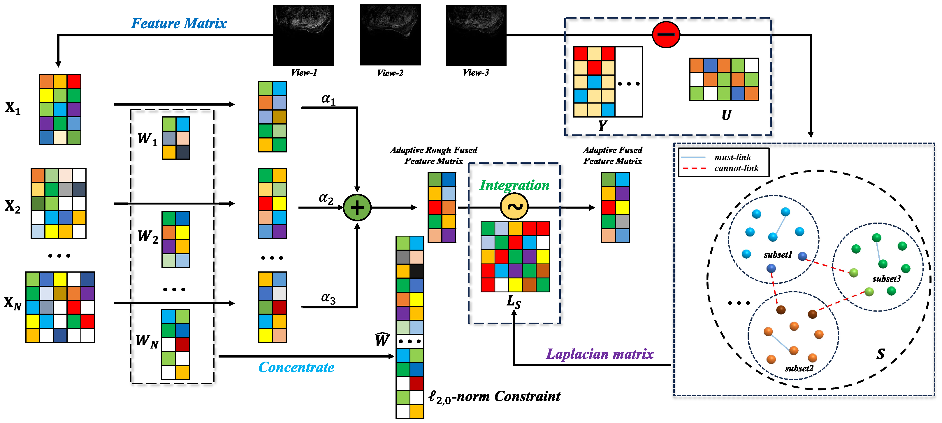
To overcome the abovementioned issues, in this paper, we aim to propose a new weakly supervised multi-view feature selection method by utilizing pairwise constraints. Note that pairwise constraints are easy to incorporate into graph-based clustering methods. Thus, we formulate the multi-view feature selection model by simultaneously performing pairwise constrained similarity learning and view-specific sparse projection. In this manner, the pairwise constraint information and local structure information can be fully explored to facilitate discriminative projection learning. To select an exact number of features, the -norm-based row sparsity constraint is adopted instead of the -norm in most existing works. That is to say, the -norm-based row sparsity constraint is imposed on the concatenated projection of all views. Then, the features that correspond to the non-zero rows of the concatenated projection matrix are selected. The resultant model is referred to as the pairwise constrained multi-view feature selection method, which is named PCFS for short hereinafter. The workflow of PCFS is shown in Figure 1.

Figure 1.
This is the workflow of PCFS, where the sample images come from Ref. [29].
In summary, the major contribution of this paper is that a new weakly supervised multi-view feature selection method is proposed. The proposed PCFS method makes full use of pairwise constraints to boost the feature selection performance, which are overlooked by existing multi-view feature selection methods. To be specific, the contributions of this paper can be refined as follows:
- A common pairwise constrained similarity matrix for all views is adaptively learned, which exploits both the pairwise constraint information and local structure information to help select discriminative features.
- View-specific projections are optimized under the -norm-based cross-view sparsity constraint on the concatenated projection. In this way, both the consistent and complementary information of multiple views can be well captured.
- An iterative algorithm was designed to optimize the objective function of the proposed PCFS method. Systematic experiments were conducted to verify its effectiveness.
The remaining contents of this paper are organized as follows. Some related works and preliminary knowledge are reviewed in Section 2. The PCFS model, including its formulation and optimization, is described in Section 3. In Section 4, we present the conducted experimental studies used to evaluate the effectiveness of PCFS. In Section 5, PCFS was applied to two cancer datasets. Section 6 gives a conclusion of this paper and Section 7 puts forward future work.
2. Related Works
In this section, we first introduce the notations and state the problem setting. Then, we review some representative unsupervised multi-view feature selection methods.
2.1. Notations and Problem Statement
Throughout this paper, we utilize boldface lowercase letters to denote vectors and matrices are written in boldface uppercase letters. For a matrix , its -th element is denoted as and its i-th row and j-the column are denoted by and , respectively. The -norm of is defined as , where the operation outputs 1 if the input scalar is non-zero, and 0 otherwise. The -norm of is defined as . It can be seen that the -norm-based minimization of a matrix can achieve row sparsity. The -norm is the convex approximation of the -norm. denotes the trace of the matrix when is square. denotes the Frobenius norm of and denotes the transpose of .
Assume that we are given a multi-view dataset with n samples and V views, where each view is denoted as and is the i-th sample of the v-th view. The concatenated feature matrix is denoted as . The goal of unsupervised multi-view feature selection is to select the k most discriminative features from the original d features, where . Some important notations and their specific descriptions are documented in Table 1.

Table 1.
Notations.
2.2. AMFS
Adaptive multi-view feature selection (AMFS) [19] is an unsupervised feature selection method proposed for human motion retrieval. AMFS employs local descriptors to characterize the local geometric structure of human motion data. AMFS can select discriminative features in three steps. First of all, it generates the Laplacian graph [30] as a local descriptor for each single view. After this, these Laplacian matrices are combined together with nonnegative view weights to explore more complementary information between different views. Finally, trace ratio criteria, as in the traditional Fisher score feature selection method, are used in AMFS to discard the redundant features.
In general, the objective function of AMFS is formulated as follows:
where is the Laplacian graph corresponding to the v-th view and is the centralized matrix to centralize the data points. is the weight coefficient vector used to combine the different Laplacian matrices and means that its elements are all nonnegative. The parameter is designed to avoid the trivial solutions. is a weight coefficient matrix that has one and only one non-zero element in each row for realizing feature selection. The features corresponding to non-zero elements are naturally selected.
2.3. ASVW
Adaptive similarity and view weight (ASVW) [24] assumes that all the similarity matrices between different views are selfsame for characterizing the common structure from data points in all views. ASVW learns the common similarity matrix from the given multi-view data rather than using the predefined one. Considering that nearby points in high-dimensional space should also be nearby in low-dimensional space, the objective function of ASVW is described as follows:
where is a nonnegative balance parameter, is the m-order identity matrix, is the p-th power of the -norm of , and . has the same meaning as in AMFS, and and are two parameters used to avoid trivial solutions. means that each sample is only connected with neighbors. ASVW evaluates the importance of all features from different views with the two-norm of after deriving the best optimal solution.
2.4. RMVFS
Robust multi-view feature selection (RMVFS) [23] is a model based on multi-view K-means. Concretely, it first produces pseudo-labels obtained by robust multi-view K-means. Then, the feature matrices of multiple views are projected to the aligned-label-indicating matrix with sparsity regularization. The optimization problem of RMVFS can be summarized as follows:
where is regarded as the corresponding centroid matrix of the v-th view and is the label alignment matrix. An alternate K-means-like optimization solution is utilized to update the variables in the unified framework.
2.5. JMVFG
Joint multi-view unsupervised feature selection and graph learning (JMVFG) [25] is an approach based on orthogonal decomposition. Given multi-view data feature matrices and initial similarity matrices , JMVFG decomposes into view-specific basis matrices and a view-consistent cluster indicator matrix . Moreover, the unified similarity matrix is adaptively constructed with the mutual collaboration of the global multi-graph fusion to ensure the cross-space locality preservation mechanism. On the whole, the objective function of JMVFG can be formulated as follows:
where , , and are hyperparameters that control the weights of the regularization term, the cross-space locality preservation term, and the graph term, respectively. is an automatic learnable parameter that measures the importance of each view during the optimization. is a vector with all ones, and is the identity matrix. In the rest of this paper, the dimensionality of and the order of are omitted when there is no confusion.
3. Methodology
In this section, we introduce the proposed PCFS method, including its model construction and the optimization algorithm.
3.1. The Model of PCFS
Given a multi-view dataset , and the corresponding pairwise constraints, the goal of PCFS is to select the k most discriminative features from the original d features. To be specific, the set of must-link and cannot-link constraints are represented as and . Concretely,
We adopted sparse projection to formulate the model. During the projection process, in order to preserve the local similarity, it usually requires that nearby points in the original space should be near in the projected space. Thus, the initial model can be formulated as
where is the adaptively optimized similarity between and , is the weight that reflects the contribution of the v-th view and , is the v-th projection matrix, and m is the dimensionality of the projected space. With the -norm-based regularization, the features can be ranked according to the -norm of , and is a trade-off parameter.
Note that this model considers each view independently and ignores the connection between multiple views. To capture the consistent information across views, it is usually assumed that multiple views share the same similarity matrix . Moreover, to avoid the trivial solution of , the sum of elements of each row of is constrained to be 1. Then, the model is updated using
where is the i-th row of and is a predefined parameter to specify the connected neighbors of each sample.
It can be seen that the above formulation falls into the parallel model category. It needs to artificially decide the number of selected features for each view. However, there still lacks a practical criterion for allocating the number of selected features for each view. To address this problem, we aim to learn a weighted low-dimensional representation. Then, we have
where and is the total dimensionality.
Rewriting the above formulation into a matrix form, it becomes
where
is the graph Laplacian. The first term of Equation (9) makes sure that the weighted low-dimensional representation preserves the original local geometric structure. The second term ranks the cross-view features as a whole. In this way, the complementary and consistent information of each view is well captured and the features are evaluated together.
Recently, Wu et al. [15] developed a technique to deal with the -norm optimization problem. This technique can be adopted to obtain a feature selection model with strict row sparsity. To be specific, the model is improved using
where k is the number of selected features and is the m-th-order identity matrix.
Since prior pairwise constraints reflect the relationship between sample pairs, it is natural to represent them with the graph similarity. If there is a must-link between and , this is equivalent to . However, simply letting cannot guarantee that and are in different connected components since there might be indirect path between and . To overcome this issue, we adopted the graph-Laplacian-based cannot-link regularization proposed in [31].
Theorem 1
([31]). Denote the similarity matrix as . For a cannot-link constraint between and , its indicator vector is defined as and . If
then and must be in different connected components of .
According to Theorem 1, the formulation of PCFS can be further improved using
where () is the indicating vector of the t-th cannot-link , , is a given small positive value, and is a parameter used to balance the local-structure-preserving term and the cannot-link regularization term.
Meanwhile, as indicated in recent work [32], a theoretically ideal similarity matrix should have the property that the number of connected components equals the number of clusters. Such a property is also preferred in feature selection methods based on similarity learning [21]. If there are c connected components in a graph with n vertexes, then the rank of the graph Laplacian will equal . Note that the rank of can be judged from its eigenvalues. Denote the j-th smallest eigenvalue of as ; then, leads to . According to Ky Fan theory [33],
Thus, when is large enough, the rank constraint can be realized by optimizing
which is the optimization problem of the proposed PCFS. It can be seen that PCFS leverages consistent and complementary cross-view information by the common similarity matrix and weighted combination of view-specific projections, respectively. When learning the common similarity matrix, pairwise constraints are incorporated to provide prior information.
3.2. Optimization of PCFS
There are five groups of variables to be optimized in problem (15). We considered designing an iterative algorithm to optimize them.
Moreover, it can be turned into
where is a diagonal matrix, , , and . is the diagonal vector of and is the vector diagonal operator. If we let , it can be written as
Furthermore, we denote , where should be large enough to guarantee that is a positive semi-definite matrix. Then, problem (17) can be written as
which is an NP-hard problem. Then, we consider solving it using two cases. First, we discuss the case . Since , let be the indicator vector of non-space rows of and be an indicator vector that selects k unduplicated elements from in an ascending order. Then, can be decomposed into , where ; the element of H equals 1 only if ; and is the mapping function . Naturally, , such that problem (18) can be written as the following problem (19):
where the optimal , and is an indicator vector of representations of the first k maxima of the diagonal vector of the . Then, in problem (19), the solution can be obtained by the eigenvectors corresponding to the first m maximum eigenvalues of . Finally, can be calculated as .
On the other side, we consider the case . In this case, we consider utilizing the famous Majorize–Maximization (MM) framework [34]. Suppose the current solution is . Through observing , where is the Moore–Penrose inverse operator, we guess the following surrogate problem of problem (18) based on the MM framework:
with the following theorem.
Theorem 2
Then, we can suppose that problem (20) can be a surrogate problem for problem (18). Afterward, we focus on the surrogate problem (20) and draw the following two conclusions: (1) Since , we have . (2) Considering is positive semi-definite, we have
Therefore, the positive semi-definite is obtained. Therefore, problem (20) can be solved in the same way as problem (18) in the case of . For conciseness, we do not provide the detailed optimization procedures.
(ii) Update and fix the others. When , and are fixed, model (15) becomes
Considering that the independence between the columns of , problem (22) can be achieved by solving
As stated before, the optimization of can be regarded as the label propagation process over the graph [35]. To be specific, we rearrange all samples as . According to the reference above, the rearranged is expressed as , where . Naturally, is also rearranged into , whose Laplacian matrix is turned into . Therefore, problem (23) can be reformulated as
Then, according to the label propagation algorithm [35], the closed-form solution to problem (24) is .
(iii) Update and fix the others. When , and are fixed, model (15) becomes
Problem (25) degrades to a spectral clustering problem [36], whose solution consists of the eigenvectors of corresponding to its c smallest eigenvalues.
(iv) Update and fix the others. When , and are fixed, since every part of the model (15) contains the Laplacian matrix , we denote such that model (15) becomes
where .
To address the problem above, we introduce a property in the spectral analysis [36] described as
Afterward, problem (26) can be reformulated as
where , and . We note that the optimal solution to problem (28) should basically maintain the similarity with the original matrix, which is directly preconstructed by neighbor data points. Therefore, we assume that the current unoptimized similarity matrix is . To avoid confusion, let . Then, the optimal solution to problem (28) should also be the solution to the following problems:
Considering that each column of is independent, we can address problem (29) by solving the following problem for each column:
where . According to , the must-linked objects of the i-th samples are denoted as . Fix and , and denote , and as , and , respectively. Then, problem (30) can be rewritten as
where denotes the number of elements in . The above problem (31) can be efficiently addressed by referring to Reference [37] under the KKT condition. The Lagrangian function of problem (31) is
where and are Lagrangian multipliers. This is obviously the converged solution of problem (31) satisfying the KKT condition. Based on this, the optimal solution of is
where , and [32].
Without loss of generality, we suppose are ordered from smallest to largest. Thus, the optimal solution is obtained by
The algorithm to solve model (15) is summarized in Algorithm 1.
| Algorithm 1 Algorithm to solve model (15) |
|
4. Experiments
4.1. Experimental Datasets
In this part, experiments that were performed on two different types of datasets are described. Specifically, we selected six real datasets related to images or videos to evaluate PCFS as below:
- Caltech101-7 comes from the Caltech Class 101 Image Database and it consists of 441 images from one to seven classes, which is associated with six views, namely, Gabor, WM, CENT, HOG, GIST, and LBP.
- Caltech101-20 is comprised of 2386 images belonging to 20 classes. Gabor, WM, CENT, HOG, GIST, and LBP were extracted as six views.
- AR10P includes 130 images divided into 10 categories. Each category contains 13 instances and SIFT, HOG, LBP, wavelet texture, and GIST were extracted as five views for the experiments.
- Yale contains a total of 165 images from 15 volunteers, each with 15 images. Each person corresponds to one class; thus, five features were used as five views: SIFT, HOG, LBP, wavelet texture, and GIST.
- YaleB is a dataset containing 2414 images from 38 classes. SIFT, HOG, LBP, wavelet texture, and GIST formed five views for the experiments.
- Kodak is a video dataset for the consumer domain, and all samples are from actual users. It contains 2172 samples that can be divided into 21 categories. The edge orientation histogram, Gabor texture, and grid color rectangle were divided into three views.
More details related to the datasets are directly shown in Table 2.
Table 2.
The descriptions of the experimental datasets.
4.2. Experimental Setting
Baselines: We compared PCFS with several representative multi-view feature selection methods on the clustering performance. When determining the baseline methods, we mainly considered their representativeness, diversity, and novelty. First of all, to show whether feature selection boosted the clustering performance or not, k-means with all features (ALLfea) was compared. Then, considering that the proposed PCFS method is a graph-based method, we compared it with the representative and prevalent graph-based methods: ACSL [21], ASVW [24], and AMFS [19]. Moreover, to increase the type diversity of the baselines, RMVFS [23] was selected because it is a classical multi-view feature selection method based on pseudo-label learning in a k-means-like style. Finally, considering the novelty and timeliness, we compared PCFS with JMVFG [25]. More concretely, JMVFG is a new multi-view feature selection method and it combines pseudo-label learning and graph learning to facilitate feature selection. Overall, due to the above considerations, AllFea, ACSL, ASVW, AMFS, RMVFS, and JMVFG were selected as baselines.
Evaluation metrics: We employed the standard metrics clustering accuracy (ACC) and normalized mutual information (NMI) for performance comparison. ACC is a popular metric that utilizes the permutation map function to describe the rate of accurately clustered samples to the total sample amount and is widely used to evaluate clustering performance [38]. NMI is a normalized form of mutual information (MI) using a geometric mean, which provides a credible indication of the shared information between two clustering partitions without the influence of the arrangement of cluster labels [39]. Another interesting criterion is the variation of information (VI), which is derived from information theoretic principles, the same as MI, and represents the sum of conditional entropies for comparing a pair of clusters [40]. The value of NMI ranges from 0 to 1, while VI is bounded by an upper bound that depends on the number of clusters. Therefore, NMI is more suitable than VI for comparison in our setting as a metric. ACC and NMI are the most commonly used metrics for evaluating clustering results. In [41,42,43,44], only NMI and ACC were used as evaluation metrics. Overall, ACC and NMI are cogent enough for evaluating clustering results in most cases. For both evaluation metrics, larger values indicate better performance.
Parameter setting: In our work, the number of neighbors was set to five when the KNN graph was involved in a certain method. In terms of PCFS, and were chosen from , and , respectively. For each experiment, the same key pairwise constraint that consisted of 80 cannot-link constraints and 240 must-link constraints were used in each outer loop. In our PCFS, the total reduced dimensionality was empirically selected as . For a fair comparison, all the vital parameters in the baselines were set as suggested in the original paper. The number of selected features was set to , where r is the percentage of selected features, traversed from 0.1 to 0.3, with 0.02 as the interval, and is the floor function, which returns the maximum integer value that is not greater than x.
Key pairwise constraints selection: Since excessive constraints are labor-intensive, many constraint selection methods have been proposed [45,46]. Instead, we specifically use an efficient scheme [31] for semi-supervised graph clustering. Considering that S is sparse and each sample is only connected to neighbors in the feature space, it is easy to obtain intuitive and rough “neighbors”. On this basis, we () obtained the must-link constraints by querying the “non-neighbors” of the sample and () obtained the cannot-link constraints by querying the “neighbors” of the sample. In this way, we could find key pairwise samples in the original feature space that were easily mislinked or unlinked.
4.3. Evaluations on Real Datasets
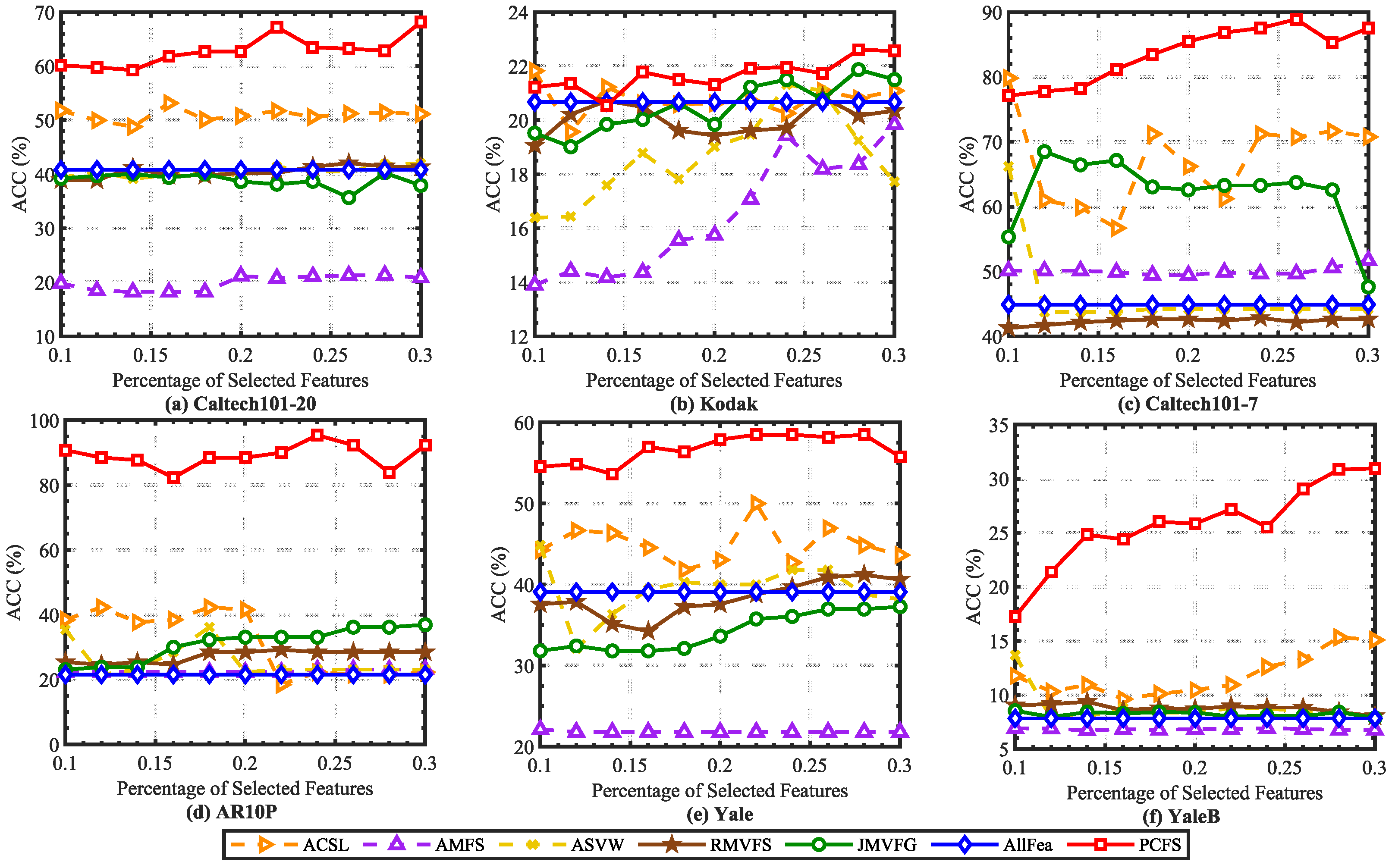
In order to alleviate the effect caused by K-means random center clustering, we predefined the cluster center by collecting the best features selected each time, and each experiment was repeated 20 times. The mean ACC and NMI scores on real datasets are reported in Figure 2 and Figure 3. It can been seen that the ACC and NMI scores grew with fluctuations when the number of selected features increased. When the scores arrived at the peak, they decreased slowly as the number of selected features continuously increased. This is consistent with intuition. By comparing the scores of different methods, it can be found that PCFS achieved a better performance than the baseline methods in most cases.
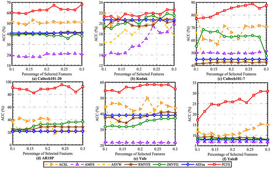
Figure 2.
Average ACC (%) scores of different baseline methods with different percentages of selected features on real datasets.
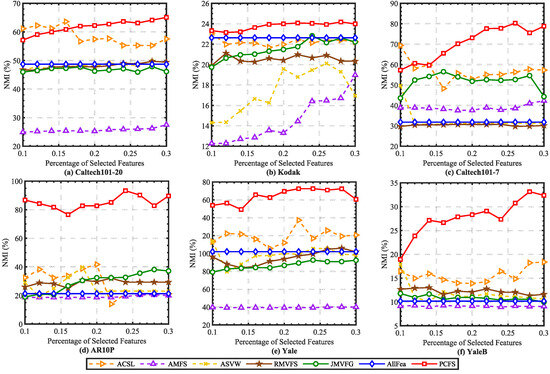
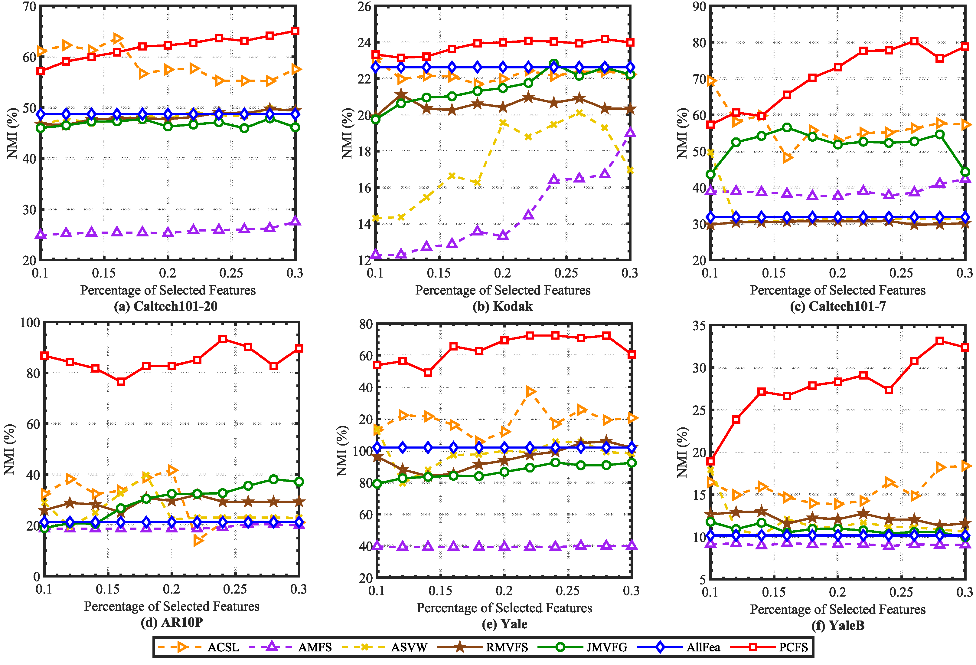
Figure 3.
Average NMI (%) scores of different baseline methods with different percentages of selected features on real datasets.
Furthermore, we show the scores of evaluation metrics of different multi-view feature selection methods on six real datasets when the percentage of selected features in Table 3. The proposed method obtained the highest ACC and NMI scores in most cases. Moreover, we utilized Student’s t-test to verify the statistical significance of the results. The symbols “*” and “†” indicate significant improvement and reduction in PCFS over the corresponding baseline method, respectively, with . On Kodak, Caltech101-20, and Caltech101-7, as shown in Table 3, PCFS had a slightly lower evaluation score than ACSL when . However, as Figure 2 and Figure 3 show, with the increase in r, the evaluation score of PCFS exceeded that of ACSL, and the result was more robust than that of ACSL on the whole. The results of the Student’s t-test also show that the improvement in PCFS compared with ACSL was significant when r varied in the region of 0.1 to 0.3. Overall, the robust and high performance of PCFS is fully demonstrated in Table 3 and Figure 2 and Figure 3.
Table 3.
The average performance (mean ) was obtained from 20 runs in each multi-view feature selection algorithm. The best score on each dataset is highlighted in bold. The symbols “*” and “†” indicate significant improvement and significant reduction in the proposed method over the baseline on the dataset with , respectively. And no special marks are given for those with no significant difference.
4.4. Convergence Analysis
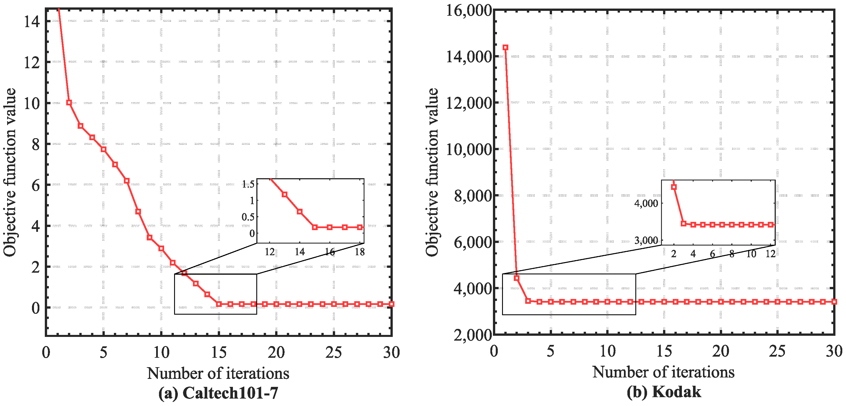
In this section, we conduct empirical convergence analysis on the real datasets. According to the theoretical analysis in the Methodology section, the monotonicity of each step in our optimization algorithm could be guaranteed. Specifically, we illustrate the convergence curves of PCFS in Figure 4. We can easily observe that the objective value rapidly and monotonically decreased as the number of iterations grew, where the convergence curves became stable within about 10 iterations. The fast convergence ensured the optimization efficiency of PCFS.
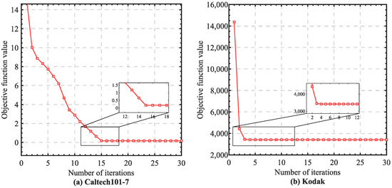
Figure 4.
Empirical convergence analysis. The objective function value of PCFS is illustrated as the number of iterations increased.
4.5. Parameter Analysis
First of all, let us theoretically discuss the effects of the parameters , and . represents a constant that sets weights for the edges between instances that must be linked. As the connectivity of the graph is independent of the edge weights [31], the value of has no direct impact on our model’s performance. With regard to , it has been established that a sufficiently large guarantees that is an ideal similarity matrix, and how large the value of is considered enough needs to be discussed further in the experiments. Considering , as , the pairwise constraints regularization term approaches zero infinitely, and all cannot-link constraints will be satisfied. However, too strict cannot-link constraints regularization will lead to very meticulous spectral clustering results, and it may be more difficult to select important and vital features, which affects the accuracy of the following k-means clustering with selected features. Therefore, should be appropriate, i.e., neither too small nor too large.
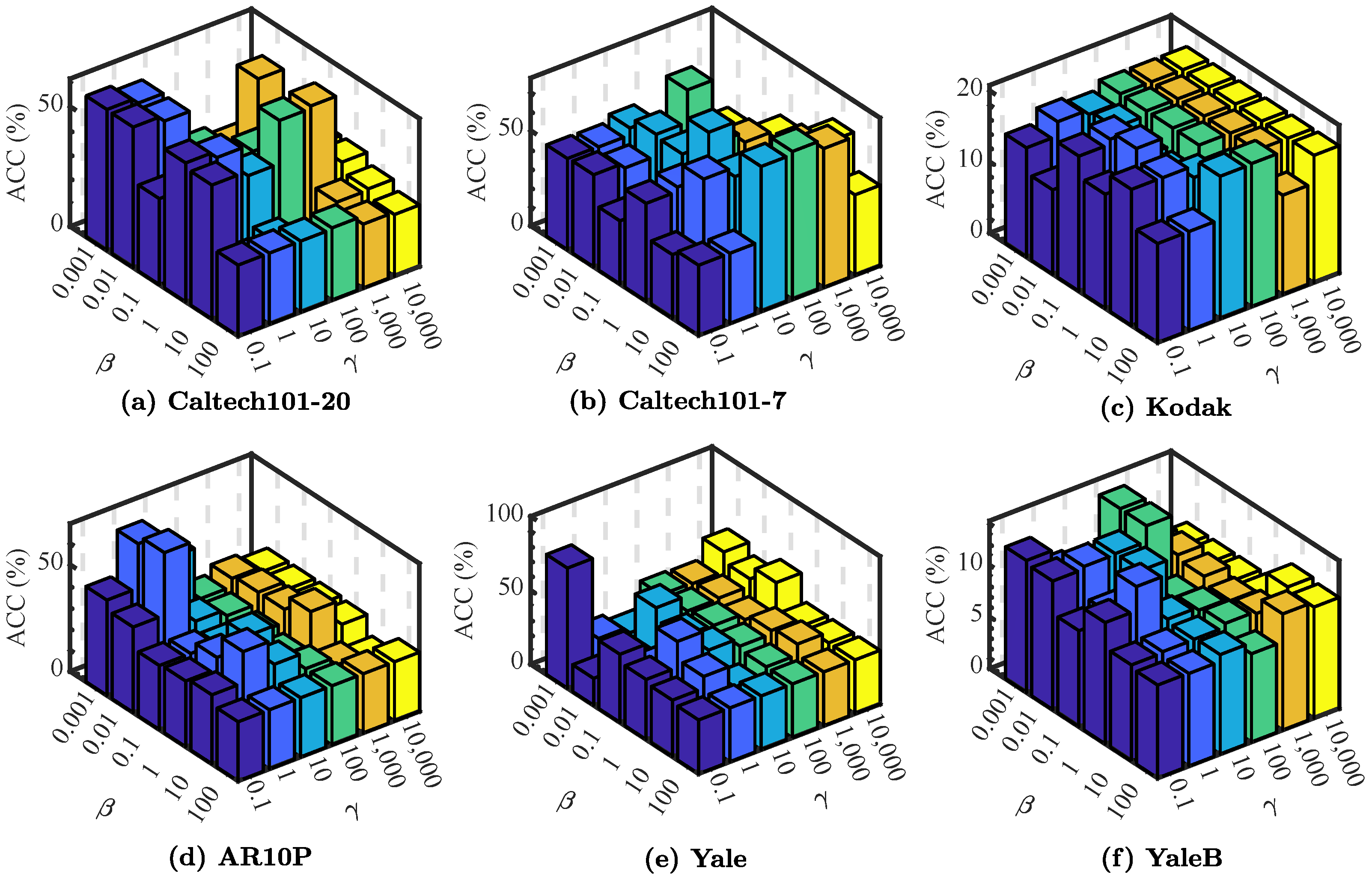
Then, as we emphasized, the results of the experiments designed to analyze the influence of and directly show that the variability of the two parameters and have important impacts on the performance of our model. Specifically, the performance of our method with varying parameters and and fixing is illustrated in Figure 5. As shown in it, the performance of the proposed method fluctuated with some hidden regularity, which suggests that the selection of needed to be careful and delicate and the selection of should not be too large. Small changes in will cause the pairwise constraints to have a drastic impact on the results. Within a certain range, the increase in will increase the score, but it will be counterproductive after exceeding this range. The selection requirements of these two parameters actually reflect the requirements of two different constraints on the graph. Our method needs to find a balance point from which to obtain high-quality performance on most of the datasets.
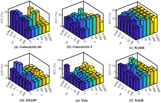
Figure 5.
The average performance (with respect to ACC (%)) scores of PCFS with varying and while fixing .
4.6. Ablation Study
This section describes the ablation analysis of the proposed PCFS method. There are two regularization terms in the objective function of PCFS. They are the cannot-link regularization related to the cannot indicating matrix and the Laplacian rank regularization related to . We compared PCFS with its variants with the cannot-link regularization or the Laplacian rank regularization removed. The results are shown in Table 4. It can be seen that the complete PCFS method using all regularization terms led to average and scores (over six datasets) of 62.86% and 64.63%, respectively.
Table 4.
Average performances (mean ) over 20 runs by different methods on each dataset; the best score is highlighted in bold.
On average, when the cannot-link regularization term was removed, the corresponding and scores were the lowest. This demonstrated that pairwise constraints were beneficial for multi-view feature selection from the opposite side. From the results of each dataset, it can be seen that only using the Laplacian rank regularization obtained lower scores than the model without any regularization terms. The possible reason for this was that excessive attention on the graph Laplacian rank led to inaccurate similarity learning. The utilization of pairwise constraints helped to prevent such deterioration, and thus, PCFS achieved a better performance.
4.7. Discussion
We tried to understand the performance of PCFS from two aspects. First, we conducted a comparison of PCFS with six baseline methods on six widely used multi-view datasets. The comparison results demonstrate the effectiveness of the proposed PCFS method. Second, we conducted ablation experiment to analyze the function of each part of the objective of PCFS. The ablation experiment results show that the proper integration of pairwise constraints and graph rank regularization helped to improve the multi-view feature selection performance.
In other published papers, Refs. [31,47] integrated pairwise constraints into the single-view clustering method and concluded that including pairwise constraint information considerably improves the clustering performance. Ref. [48] also tried to introduce pairwise constraints in multi-views data and obtained consistent results. In our work, the pairwise constraints were introduced into the similarity graph learning and combined with the row sparse projections based on the -norm to finally fulfill the multi-view feature selection task. Our work was a fusion and extension of the existing work, and theoretically had the ability to improve the clustering performance. The final experimental results also demonstrate that the findings of our work are in line with previous related works. Pairwise constraints helped the multi-view feature selection and improved its clustering performance.
5. Application on Cancer Datasets
Two multi-omics cancer datasets obtained from The Cancer Genome Atlas (TCGA) were used for the evaluation.
BRCA (breast invasive carcinoma) [49] consists of 398 samples belonging to four categories. It has four different views, namely, gene expression (RNA), mitochondrial DNA (mDNA), microRNA expression (miRNA), and reverse phase protein array expression (protein), which are measured on different platforms and contain different biological information.
CESC (cervical carcinoma) [50] consists of 128 samples which come from three different categories. Gene expression (RNA), mitochondrial DNA (mDNA), microRNA expression (miRNA), and reverse phase protein array expression (protein) contain different information and are measured on different platforms. Thus, the information naturally formed four different views for experiments.
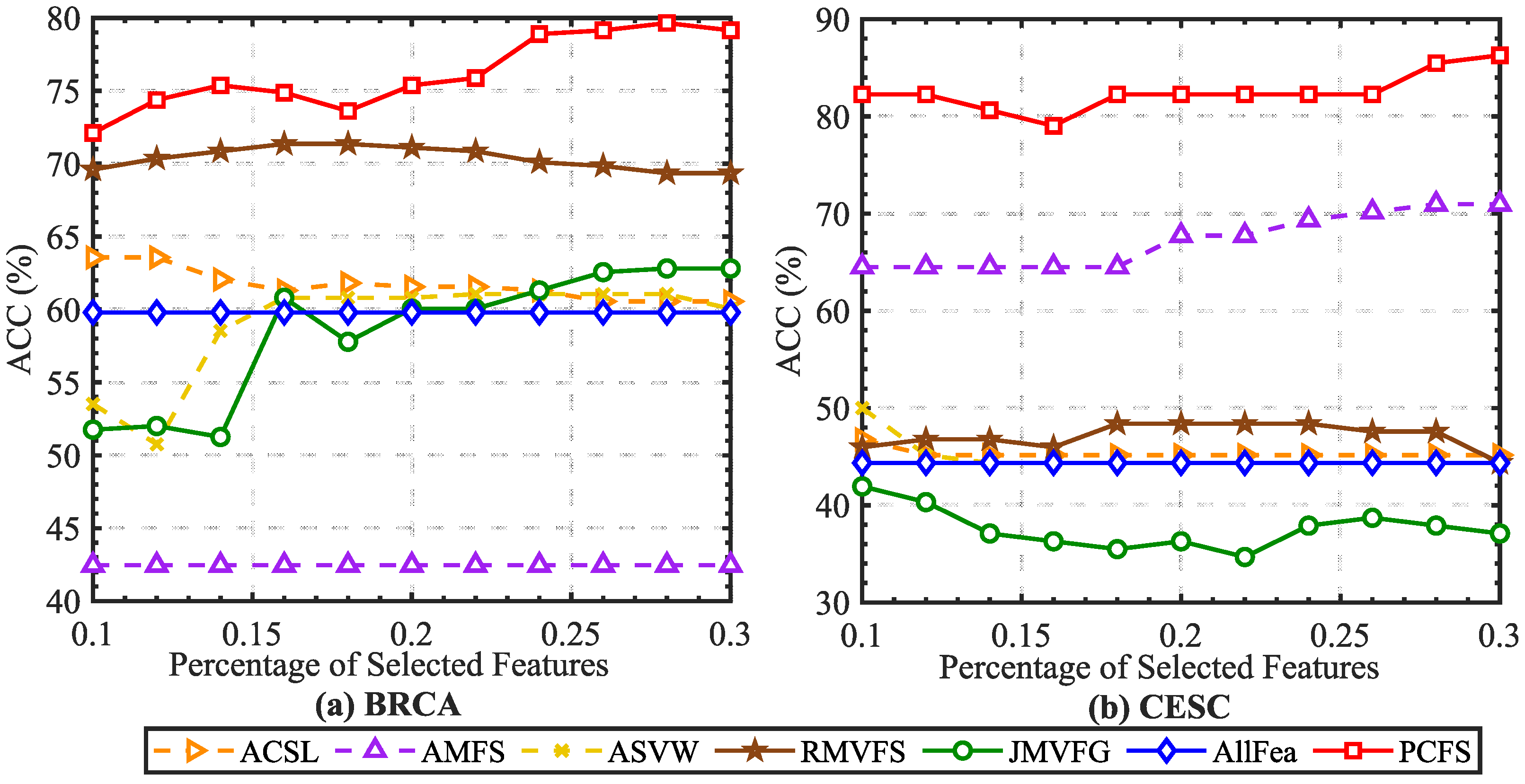
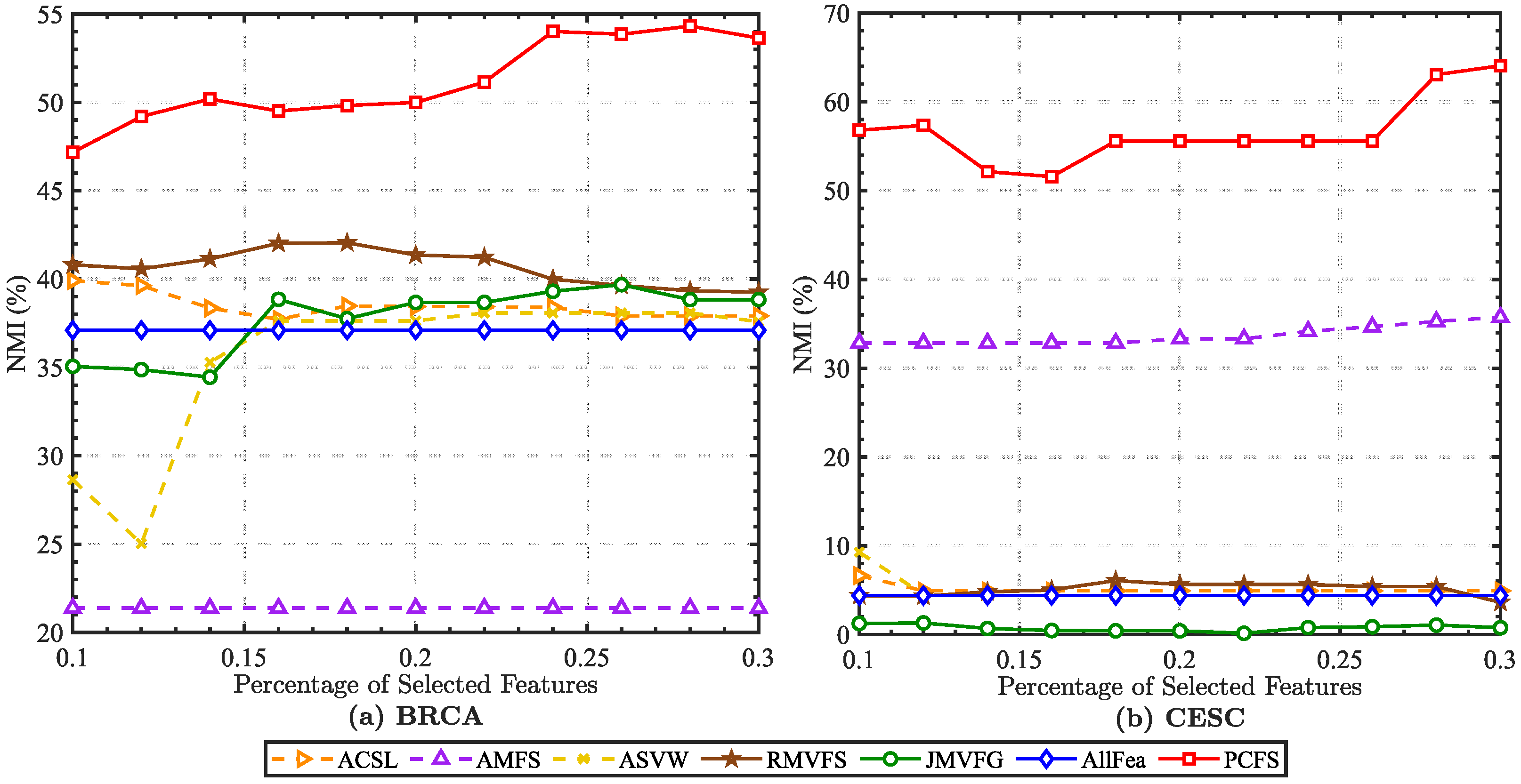
The experimental setting was kept consistent with Section 4. By using the selected features to predefine the cluster center, we obtained the performance of each method on the multi-omics cancer datasets. According to the average ACC and NMI scores shown in Figure 6 and Figure 7, our proposed method achieved excellent performances on these two datasets. It should be noted that for the BRCA dataset, we preprocessed the original dataset with the -norm, while the CESC dataset was preprocessed with the -norm. With either preprocessing method, the proposed method showed robust and excellent performances on both two datasets. More details are directly shown in Table 5.
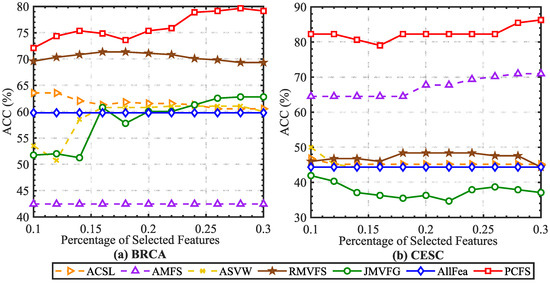
Figure 6.
Average ACC (%) scores of different baseline methods with different percentages of selected features on cancer datasets.
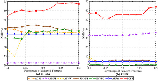
Figure 7.
Average NMI (%) scores of different baseline methods with different percentages of selected features on cancer datasets.
Table 5.
The average performance (mean ) was obtained from 20 runs in each multi-view feature selection algorithm. On each cancer dataset, the best score is highlighted in bold. The symbol “*” indicates significant improvement of the proposed method over the baseline on the dataset with . And no special marks are given for those with no significant difference.
6. Conclusions
In this paper, a weakly supervised multi-view feature selection method named PCFS is proposed. PCFS utilizes pairwise constraints, i.e., cannot-links and must-links, to boost multi-view feature selection, which have been overlooked by most of the existing methods. The performance of this method was evaluated by comparison with related methods on six widely used multi-view datasets and two cancer datasets. The proposed PCFS method outperformed the baselines in most cases. This demonstrates that PCFS has promising multi-view feature selection performance.
7. Future Work
From the theoretical aspect, studying how to integrate pairwise constraint propagation into the proposed PCFS method is possible future work. Then, more pairwise constraints can be inferred, thereby benefiting the feature selection process. From the application aspect, the proposed PCFS method can be applied to crop disease image recognition [51] and histopathology image classification [52] to select prominent features.
Author Contributions
Methodology, J.L.; validation, J.L.; data curation, J.L.; resources, H.T.; writing—original draft, J.L. All authors have read and agreed to the published version of the manuscript.
Funding
This work was supported in part by NSF of China under grant 62006238 and in part by the NSF of Hunan Province under grant 2023JJ20052.
Data Availability Statement
No new data were created or analyzed in this study. Data sharing is not applicable to this article.
Conflicts of Interest
The authors declare no conflicts of interest.
References
- Khan, A.; Maji, P. Selective update of relevant eigenspaces for integrative clustering of multimodal data. IEEE Trans. Cybern. 2020, 52, 947–959. [Google Scholar] [CrossRef] [PubMed]
- Ojala, T.; Pietikainen, M.; Maenpaa, T. Multiresolution gray-scale and rotation invariant texture classification with local binary patterns. IEEE Trans. Pattern Anal. Mach. Intell. 2002, 24, 971–987. [Google Scholar] [CrossRef]
- Dalal, N.; Triggs, B. Histograms of oriented gradients for human detection. In Proceedings of the 2005 IEEE Computer Society Conference on Computer Vision and Pattern Recognition (CVPR’05), San Diego, CA, USA, 20–25 June 2005; Volume 1, pp. 886–893. [Google Scholar]
- Lowe, D.G. Distinctive image features from scale-invariant keypoints. Int. J. Comput. Vis. 2004, 60, 91–110. [Google Scholar] [CrossRef]
- White, M.; Zhang, X.; Schuurmans, D.; Yu, Y.L. Convex multi-view subspace learning. Adv. Neural Inf. Process. Syst. 2012, 25, 1673–1681. [Google Scholar]
- Han, Y.; Yang, Y.; Yan, Y.; Ma, Z.; Sebe, N.; Zhou, X. Semisupervised feature selection via spline regression for video semantic recognition. IEEE Trans. Neural Netw. Learn. Syst. 2014, 26, 252–264. [Google Scholar]
- Duarte, M.F.; Hu, Y.H. Vehicle classification in distributed sensor networks. J. Parallel Distrib. Comput. 2004, 64, 826–838. [Google Scholar] [CrossRef]
- Cai, X.; Nie, F.; Huang, H. Multi-view k-means clustering on big data. In Proceedings of the Twenty-Third International Joint Conference on Artificial Intelligence, Beijing, China, 3–9 August 2013. [Google Scholar]
- Zhang, Y.; Wu, J.; Cai, Z.; Philip, S.Y. Multi-view multi-label learning with sparse feature selection for image annotation. IEEE Trans. Multimed. 2020, 22, 2844–2857. [Google Scholar] [CrossRef]
- Xu, C.; Tao, D.; Xu, C. A survey on multi-view learning. arXiv 2013, arXiv:1304.5634. [Google Scholar]
- Sun, S. A survey of multi-view machine learning. Neural Comput. Appl. 2013, 23, 2031–2038. [Google Scholar] [CrossRef]
- Lin, Q.; Yang, L.; Zhong, P.; Zou, H. Robust supervised multi-view feature selection with weighted shared loss and maximum margin criterion. Knowl. Based Syst. 2021, 229, 107331. [Google Scholar] [CrossRef]
- Zhang, C.; Jiang, B.; Wang, Z.; Yang, J.; Lu, Y.; Wu, X.; Sheng, W. Efficient multi-view semi-supervised feature selection. Inf. Sci. 2023, 649, 119675. [Google Scholar] [CrossRef]
- Wu, J.S.; Li, Y.; Gong, J.X.; Min, W. Collaborative and Discriminative Subspace Learning for unsupervised multi-view feature selection. Eng. Appl. Artif. Intell. 2024, 133, 108145. [Google Scholar] [CrossRef]
- Wu, D.; Xu, J.; Dong, X.; Liao, M.; Wang, R.; Nie, F.; Li, X. GSPL: A Succinct Kernel Model for Group-Sparse Projections Learning of Multiview Data. In Proceedings of the International Joint Conference on Artificial Intelligence, Montreal, QC, Canada, 19–27 August 2021. [Google Scholar]
- Zhao, Z.; Liu, H. Spectral feature selection for supervised and unsupervised learning. In Proceedings of the 24th International Conference on Machine Learning, Corvalis, OR, USA, 20–24 June 2007; pp. 1151–1157. [Google Scholar]
- Zhao, Z.; Wang, L.; Liu, H. Efficient spectral feature selection with minimum redundancy. In Proceedings of the AAAI Conference on Artificial Intelligence, Atlanta, GA, USA, 11–15 July 2010; Volume 24, pp. 673–678. [Google Scholar]
- Li, X.; Zhang, H.; Zhang, R.; Liu, Y.; Nie, F. Generalized Uncorrelated Regression with Adaptive Graph for Unsupervised Feature Selection. IEEE Trans. Neural Netw. Learn. Syst. 2019, 30, 1587–1595. [Google Scholar] [CrossRef] [PubMed]
- Wang, Z.; Feng, Y.; Qi, T.; Yang, X.; Zhang, J.J. Adaptive multi-view feature selection for human motion retrieval. Signal Process. 2016, 120, 691–701. [Google Scholar] [CrossRef]
- Feng, Y.; Xiao, J.; Zhuang, Y.; Liu, X. Adaptive unsupervised multi-view feature selection for visual concept recognition. In Proceedings of the 11th Asian Conference on Computer Vision, Daejeon, Republic of Korea, 5–9 November 2012; Springer: Berlin/Heidelberg, Germany, 2013; pp. 343–357. [Google Scholar]
- Dong, X.; Zhu, L.; Song, X.; Li, J.; Cheng, Z. Adaptive Collaborative Similarity Learning for Unsupervised Multi-view Feature Selection. arXiv 2019, arXiv:1904.11228. [Google Scholar]
- Qian, M.; Zhai, C. Unsupervised feature selection for multi-view clustering on text-image web news data. In Proceedings of the 23rd ACM International Conference on Information and Knowledge Management, Shanghai, China, 3–7 November 2014; pp. 1963–1966. [Google Scholar]
- Liu, H.; Mao, H.; Fu, Y. Robust Multi-View Feature Selection. In Proceedings of the 2016 IEEE 16th International Conference on Data Mining (ICDM), Barcelona, Spain, 12–15 December 2016. [Google Scholar]
- Hou, C.; Nie, F.; Tao, H.; Yi, D. Multi-View Unsupervised Feature Selection with Adaptive Similarity and View Weight. IEEE Trans. Knowl. Data Eng. 2017, 29, 1998–2011. [Google Scholar] [CrossRef]
- Fang, S.G.; Huang, D.; Wang, C.D.; Tang, Y. Joint Multi-View Unsupervised Feature Selection and Graph Learning. IEEE Trans. Emerg. Top. Comput. Intell. 2023, 8, 1–16. [Google Scholar] [CrossRef]
- Kumar, S.; Rowley, H.A. Classification of weakly-labeled data with partial equivalence relations. In Proceedings of the 2007 IEEE 11th International Conference on Computer Vision, Rio De Janeiro, Brazil, 14–21 October 2007; pp. 1–8. [Google Scholar]
- Cao, X.; Zhang, C.; Zhou, C.; Fu, H.; Foroosh, H. Constrained multi-view video face clustering. IEEE Trans. Image Process. 2015, 24, 4381–4393. [Google Scholar] [CrossRef] [PubMed]
- Shi, Y.; Otto, C.; Jain, A.K. Face clustering: Representation and pairwise constraints. IEEE Trans. Inf. Forensics Secur. 2018, 13, 1626–1640. [Google Scholar] [CrossRef]
- Zhao, X.; Liao, Y.; Xie, J.; He, X.; Shiqing, Z.; Wang, G.; Fang, J.; Lu, H.; Yu, J. BreastDM: A DCE-MRI dataset for breast tumor image segmentation and classification. Comput. Biol. Med. 2023, 164, 107255. [Google Scholar] [CrossRef]
- Belkin, M.; Niyogi, P. Laplacian eigenmaps for dimensionality reduction and data representation. Neural Comput. 2003, 15, 1373–1396. [Google Scholar] [CrossRef]
- Nie, F.; Zhang, H.; Wang, R.; Li, X. Semi-supervised Clustering via Pairwise Constrained Optimal Graph. In Proceedings of the 29th International Joint Conference on Artificial Intelligence, Online, 7–15 January 2021. [Google Scholar]
- Nie, F.; Wang, X.; Huang, H. Clustering and projected clustering with adaptive neighbors. In Proceedings of the KDD ’14: 20th ACM SIGKDD International Conference on Knowledge Discovery and Data Mining, New York, NY, USA, 24–27 August 2014. [Google Scholar]
- Fan, K. On a Theorem of Weyl Concerning Eigenvalues of Linear Transformations: II. Proc. Natl. Acad. Sci. USA 1950, 36, 31–35. [Google Scholar] [CrossRef] [PubMed]
- Sun, Y.; Babu, P.; Palomar, D.P. Majorization-Minimization Algorithms in Signal Processing, Communications, and Machine Learning. IEEE Trans. Signal Process. 2017, 65, 794–816. [Google Scholar] [CrossRef]
- Zhu, X.; Ghahramani, Z. Learning from labeled and unlabeled data with label propagation. In ProQuest Number: Information to All Users; Carnegie Mellon University: Pittsburgh, PA, USA, 2002. [Google Scholar]
- Ng, A.; Jordan, M.; Weiss, Y. On spectral clustering: Analysis and an algorithm. Adv. Neural Inf. Process. Syst. 2001, 14, 849–856. [Google Scholar]
- Nie, F.; Wang, X.; Jordan, M.; Huang, H. The constrained laplacian rank algorithm for graph-based clustering. In Proceedings of the AAAI conference on artificial intelligence, Phoenix, AZ, USA, 12–17 February 2016; Volume 30. [Google Scholar]
- Zhang, C.; Fu, H.; Hu, Q.; Cao, X.; Xie, Y.; Tao, D.; Xu, D. Generalized latent multi-view subspace clustering. IEEE Trans. Pattern Anal. Mach. Intell. 2018, 42, 86–99. [Google Scholar] [CrossRef] [PubMed]
- Strehl, A.; Ghosh, J. Cluster ensembles—A knowledge reuse framework for combining multiple partitions. J. Mach. Learn. Res. 2002, 3, 583–617. [Google Scholar]
- Meilă, M. Comparing clusterings by the variation of information. In Proceedings of the Learning Theory and Kernel Machines: 16th Annual Conference on Learning Theory and 7th Kernel Workshop, COLT/Kernel 2003, Washington, DC, USA, 24–27 August 2003; Springer: Berlin/Heidelberg, Germany, 2003; pp. 173–187. [Google Scholar]
- Chen, H.; Nie, F.; Wang, R.; Li, X. Unsupervised feature selection with flexible optimal graph. IEEE Trans. Neural Netw. Learn. Syst. 2022, 35, 2014–2027. [Google Scholar] [CrossRef] [PubMed]
- Wang, X.; Sun, Z.; Chehri, A.; Jeon, G.; Song, Y. A Novel Attention-Driven Framework for Unsupervised Pedestrian Re-identification with Clustering Optimization. Pattern Recognit. 2024, 146, 110045. [Google Scholar] [CrossRef]
- Yang, Z.; Zhang, H.; Liang, N.; Li, Z.; Sun, W. Semi-supervised multi-view clustering by label relaxation based non-negative matrix factorization. Vis. Comput. 2023, 39, 1409–1422. [Google Scholar] [CrossRef]
- Manojlović, T.; Štajduhar, I. Deep semi-supervised algorithm for learning cluster-oriented representations of medical images using partially observable dicom tags and images. Diagnostics 2021, 11, 1920. [Google Scholar] [CrossRef]
- Van Craenendonck, T.; Dumancic, S.; Blockeel, H. COBRA: A Fast and Simple Method for Active Clustering with Pairwise Constraints. Statistics 2018. [Google Scholar] [CrossRef]
- Xiong, S.; Azimi, J.; Fern, X.Z. Active learning of constraints for semi-supervised clustering. IEEE Trans. Knowl. Data Eng. 2013, 26, 43–54. [Google Scholar] [CrossRef]
- Wang, Y.; Chen, L.; Zhou, J.; Li, T.; Yu, Y. Pairwise constraints-based semi-supervised fuzzy clustering with multi-manifold regularization. Inf. Sci. 2023, 638, 118994. [Google Scholar] [CrossRef]
- Zhu, Z.; Gao, Q. Semi-supervised clustering via cannot link relationship for multiview data. IEEE Trans. Circuits Syst. Video Technol. 2022, 32, 8744–8755. [Google Scholar] [CrossRef]
- Khan, A.; Maji, P. Low-rank joint subspace construction for cancer subtype discovery. IEEE/ACM Trans. Comput. Biol. Bioinform. 2019, 17, 1290–1302. [Google Scholar] [CrossRef] [PubMed]
- Khan, A.; Maji, P. Multi-manifold optimization for multi-view subspace clustering. IEEE Trans. Neural Netw. Learn. Syst. 2021, 33, 3895–3907. [Google Scholar] [CrossRef]
- Gu, X.; Wang, M.; Wang, Y.; Zhou, G.; Ni, T. Discriminative semisupervised dictionary learning method with graph embedding and pairwise constraints for crop disease image recognition. Crop Prot. 2024, 176, 106489. [Google Scholar] [CrossRef]
- Tang, H.; Mao, L.; Zeng, S.; Deng, S.; Ai, Z. Discriminative dictionary learning algorithm with pairwise local constraints for histopathological image classification. Med. Biol. Eng. Comput. 2021, 59, 153–164. [Google Scholar] [CrossRef]
Disclaimer/Publisher’s Note: The statements, opinions and data contained in all publications are solely those of the individual author(s) and contributor(s) and not of MDPI and/or the editor(s). MDPI and/or the editor(s) disclaim responsibility for any injury to people or property resulting from any ideas, methods, instructions or products referred to in the content. |
© 2024 by the authors. Licensee MDPI, Basel, Switzerland. This article is an open access article distributed under the terms and conditions of the Creative Commons Attribution (CC BY) license (https://creativecommons.org/licenses/by/4.0/).