A New Generalization of the Uniform Distribution: Properties and Applications to Lifetime Data

Abstract

In this paper, we generalize two new statistical distributions, to improve the ability to model failure rates with non-monotonic, monotonic, and mainly bathtub curve behaviors. We call these distributions Generalized Powered Uniform Distribution and MOE-Powered Uniform. The proposed distributions’ approach is based on incorporating a parameter k in the power of the values of the random variables, which is associated with the Probability Density Function and includes an operator called the Powered Mean. Various statistical and mathematical features focused on reliability analysis are presented and discussed, to make the models attractive to reliability engineering or medicine specialists. We employed the Maximum Likelihood Estimator method to estimate the model parameters and we analyzed its performance through a Monte Carlo simulation study. To demonstrate the flexibility of the proposed approach, a comparative analysis was carried out on four case studies with the proposed MOE-Powered Uniform distribution, which can model failure times as a bathtub curve. The results showed that this new model is more flexible and useful for performing reliability analysis.

1. Introduction

Probability distributions are an essential topic in probability theory, due to their relevance in almost all sciences [1]. The application of probability distributions in engineering, econometrics, finance, medicine, agriculture, demography, and actuarial science, to name a few disciplines, has significantly impacted data analysis [1,2]. Using classical distributions to model and analyze real-life data is an ancient practice. However, most standard or common probability distributions need to be more flexible, to model the emerging events of the fourth industrial revolution, as modern data are diverse and complex [3]. This deficiency has allowed many researchers to develop new models to better fit real-life data, since the new distributions are considered to overcome the limitations of other existing distributions and can extract all the information from the data [4].

An essential feature of new distributions is that researchers add one or more parameters to known or commonly used distributions, to incorporate location, scale, and shape characteristics. The above allows us to more flexibly model behaviors related to survival analysis, for example, to analyze the useful life of a computer or human mortality, to analyze the failure rate of devices subject to use and deterioration, or to explain and forecast a variety of real-world events.

From an engineering point of view, reliability analysis has gained increasing importance among industries and manufacturers of various types of products, to model failure rates. However, one of the main problems with the distributions commonly used for this type of analysis is that they fail to faithfully represent the behavior of a bathtub curve, since its shape or graph resembles a “V”, “J”, or “U” [5]. In this sense, the need arises to explore alternatives with new models that allow behaviors closer to real life to be established for the assumptions of a bathtub curve.

For example, Méndez-González et al. [6] proposed a new distribution called Alpha Exponentiated Perks Distribution (AEXP) for reliability analysis applied to electronic devices to model bathtub curve-shaped failure times. Akarawak et al. [1] developed the Inverted Gompertz–Fréchet (IGoFre) distribution to model data with non-monotonic failure rates and to model both positively and negatively skewed data with increasing and decreasing risk ratios. Sindhu et al. [7] proposed the LE-Inverse Exponential (LE-IE) distribution to model increasing, bathtub-shaped, increasing–decreasing–constant, decreasing, and upside-down bathtub-shaped (or unimodal) failure rates. The authors applied their model to the failure times of mechanical components; the data analyzed was related to the times between failures that occurred in an air conditioning unit of a Boeing 720-4 airplane.

Other authors, such as El-Bar and Lima [8], have developed a general family of distributions called the Exponentiated Odd Lindley-X (EOL-X) family. The proposed model aims to incorporate the most important forms of the Hazard Function—increasing, decreasing, and bathtub—to model data in reliability engineering and medical data. The authors fitted their model to three real data sets: turbocharger failure times, survival times in breast cancer patients, and survival times in AIDS patients.

Other distributions developed for the reliability analysis or hazard rate are the Unit Generalized Exponential distribution [9], the Novel Alpha Power Fréchet distribution [10], the Marshall–Olkin Exponentiated Dagum distribution [11], the Bivariate Extended Chen distribution [12], the Marshall–Olkin Alpha Power family [13], the Lehmann Type-II (Kum–MSBL–II) distribution [14], the Odd Log–Logistic Lindley–Weibull distribution [15], the type II exponentiated half-logistic Topp–Leone–Marshall–Olkin-G family of distributions [16], and the new extended Kumaraswamy generated family of distributions [17].

Therefore, this article proposes a new family of the usual uniform distribution called Generalized Powered Uniform Distribution (GPUD); subsequently, we use the GPUD approach to generalize the Marshall–Olkin Extended Uniform distribution from Jose and Krishna [18], which we call MOE-Powered Uniform (MOE-PU) distribution. The main motivations for these new distributions lie in the following:

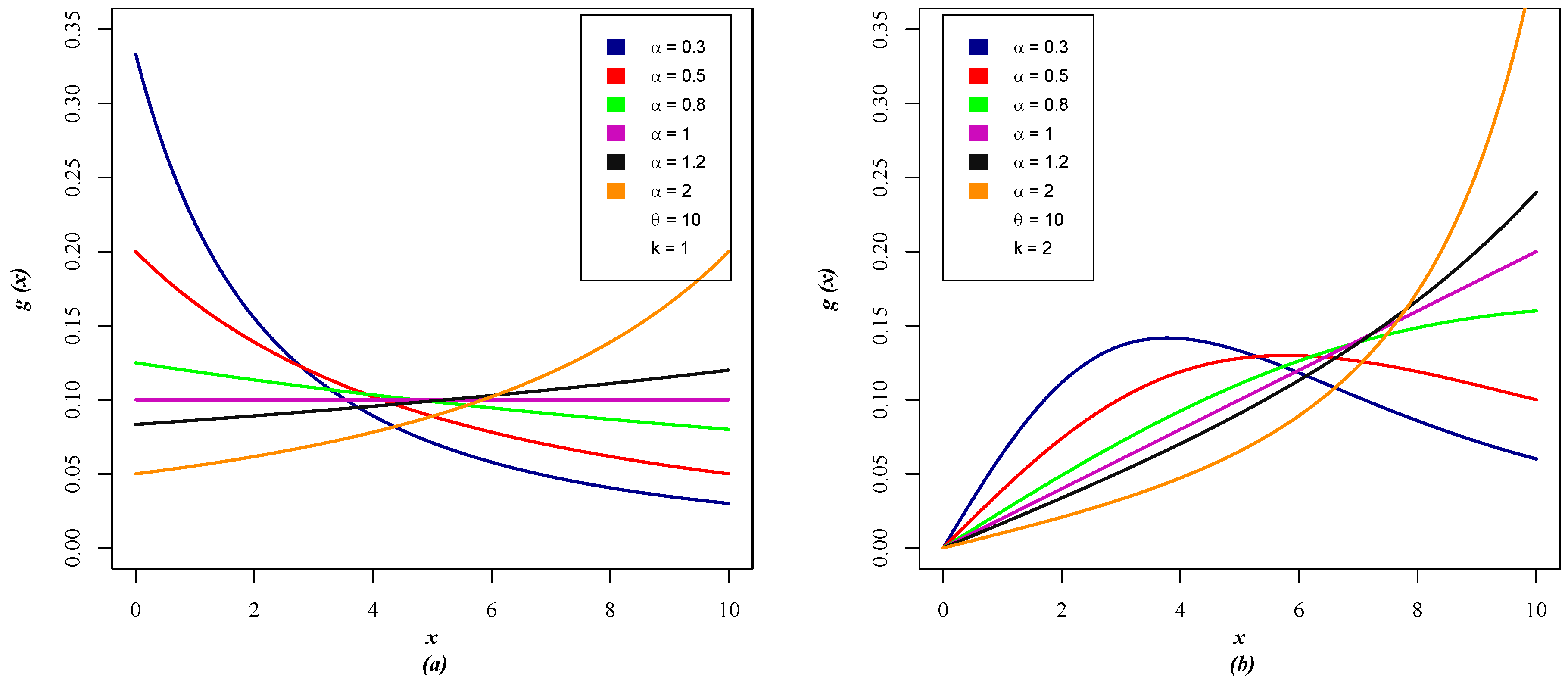
• We present an approach in which we incorporate a parameter k associated with the power of the X values of the continuous random variable in the Probability Density Function. This allows us to generalize two new distributions.
• The new GPUD distribution is presented as an alternative to the Continuous Uniform Distribution for modeling data with a uniform trend.
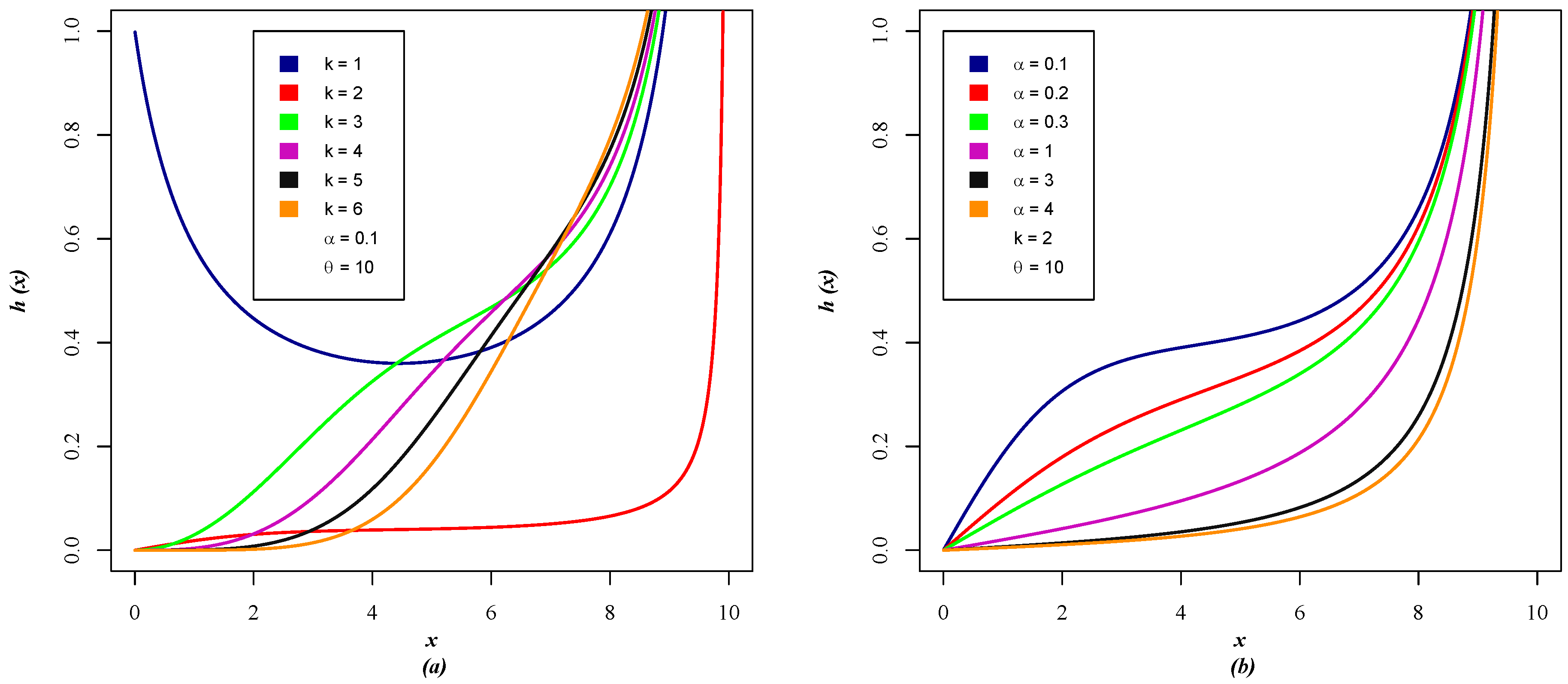
• We present the new generalized MOE-PU distribution as an alternative for reliability analysis applications that can describe non-monotonic behaviors, such as those shown by the bathtub curve.
• The MOE-PU distribution is significantly flexible and competitive with other distributions existing in the literature that can model bathtub curve behaviors.
• We establish an attractive distribution (MOE-PU) so that engineers in the reliability area can carry out different analyses or studies, considering the benefits that modeling provides from an actuarial perspective.

Finally, the structure of the paper presents the following order. In Section 2, the general conditions of the GPUD distribution, as well as some of its properties, are defined and discussed. In Section 3, the GPUD approach is used to generalize the work of Jose and Krishna [18], allowing us to generate another family of distributions (MOE-PU) for reliability analysis applications. Section 4 presents a Monte Carlo simulation study to analyze the performance of the Maximum Likelihood Estimator method. In Section 5, the case studies of the article are presented. Section 6 provides concluding comments.

2. A New Family of the Uniform Distribution Function

This paper follows the approach presented in the seminal article by Marshall and Olkin [19] and the approach by Rondero-Guerrero et al. [20]. We introduce a new parameter $\left(k\right)$ in the power of the random variables’ values, which is associated with the Probability Density Function. Our objective is to introduce a new generalization of three parameters of the usual Continuous Uniform Distribution that we call Generalized Powered Uniform Distribution, in such a way that the Probability Density Function (PDF) is defined as

$$f_{X^k}\left(x\right)=\left\{\begin{array}{ccc}{\displaystyle \frac{x^k}{(b-a)M_k(a,b)}},& a\le x\le b;\hfill & k=0,1,2,\dots ,n.\hfill \\ \\ 0,& x<a;x>b\hfill \end{array}\right.$$

(1)

where a is a location parameter, b is a scale parameter, and k is a shape parameter. The operator $M_k(a,b)$, here called the Powered Mean, is defined as follows:

$$M_k(a,b)={\displaystyle \frac{{\sum }_{j=0}^k{a}^{k-j}{b}^j}{k+1}}.$$

(2)

The Cumulative Distribution Function (CDF) corresponding to Equation (1) is given as

$$F_{X^k}\left(x\right)=P(X\le x)=\left\{\begin{array}{ccc}0,& x<a\hfill & \\ \\ {\displaystyle \frac{x^{k+1}-a^{k+1}}{b^{k+1}-a^{k+1}}},& a\le x\le b;\hfill & k=0,1,2,\cdots ,n.\hfill \\ \\ 1,& x>b\hfill \end{array}\right.$$

(3)

When $k=0$, $M_0(a,b)=1$, the classical model of the Continuous Uniform Distribution is obtained; that is, we obtain the PDF $\left(f\left(x\right)={\displaystyle \frac{1}{b-a}}\right)$ and its corresponding CDF $\left(F\left(x\right)={\displaystyle \frac{x-a}{b-a}}\right)$.

This new GPUD includes a family of polynomial functions corresponding to the PDF and CDF, respectively. Obviously, $F_{X^k}^{\prime }\left(x\right)=f_{X^k}\left(x\right)$ is satisfied.

When we set the random variable X in the interval $[0,1]$, the following is obtained:

$$F_{X^k}\left(x\right)=x^{k+1},\mathrm{for}k=0,1,2,\cdots ,n.$$

(4)

Thus, the Survival Function is expressed as

$${\overline{F}}_{X^k}\left(x\right)=1-F_{X^k}\left(x\right)=1-x^{k+1}.$$

(5)

Concerning the Powered Mean operator, some relevant properties can be mentioned, such as $M_k(0,1)={\displaystyle \frac{1}{k+1}}$ and $M_k(0,b)={\displaystyle \frac{b^k}{k+1}}$, among others.

Figure 1 shows the graphs of the PDF and the CDF of the GPUD distribution; these graphs are presented for values of $a=2$, $b=5$, and different values of the parameter k. When $k=0$, the same graph (FDP and CDF) or behavior as the usual uniform distribution is obtained. However, for values of $k>0$, the PDF form presents an increasing behavior; that is, the parameter k allows modeling data with an increasing uniform trend. It is important to remember that the CDF is represented by points on the curve (line) and not the area under the curve, which allows us to search for a probability associated with a given value of x. In this sense, for the CDF of the GPUD model, the higher the value of k, the lower the accumulated probability for a given value of x.

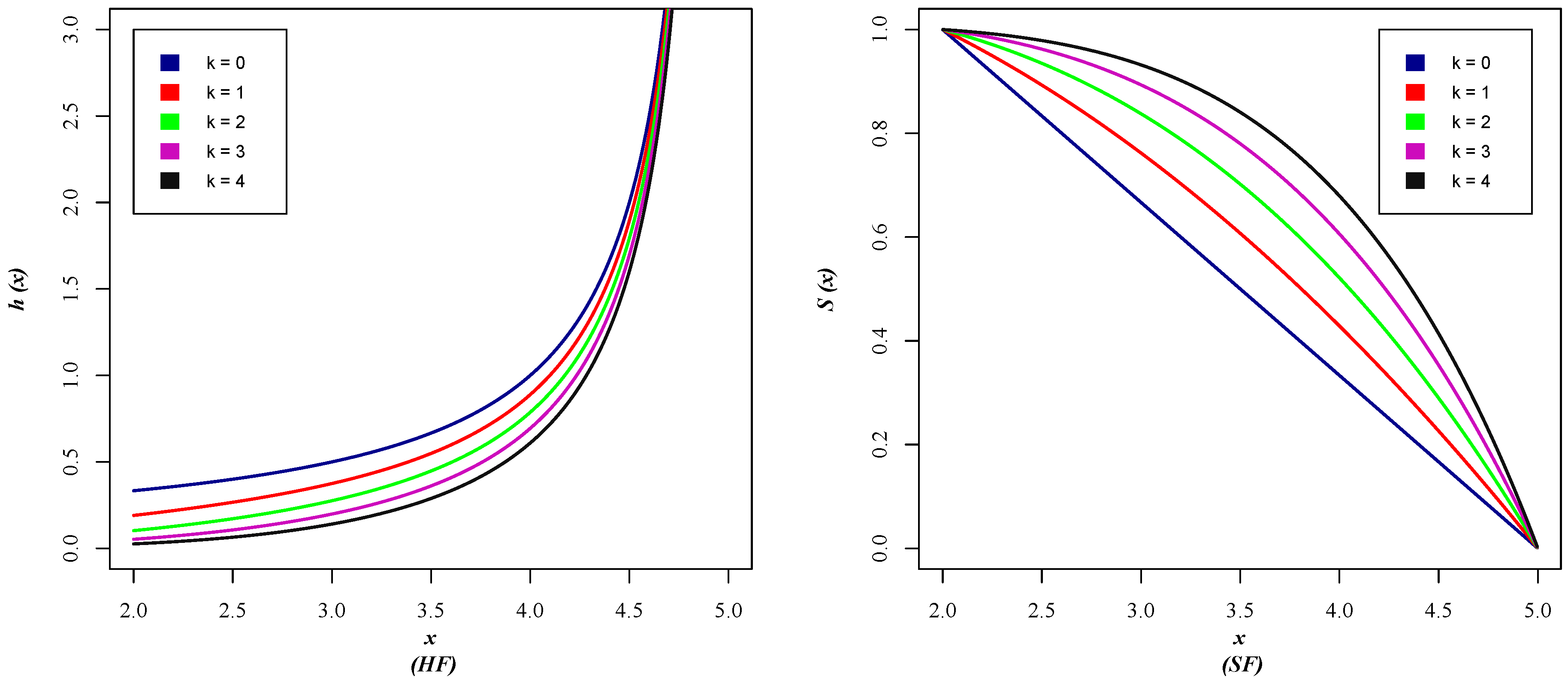
2.1. Reliability Measures of GPUD

As is known, the hazard rate and survival functions are essential in various engineering, health, and finance applications. From the GPUD perspective, both functions are shown below.

The Hazard Function (HF) can be written as

$$h_{X^k}\left(x\right)={\displaystyle \frac{f\left(x\right)}{{\overline{F}}_{X^k}\left(x\right)}}={\displaystyle \frac{x^k}{(b-a)M_k(a,b)}}·{\displaystyle \frac{1}{1-\left(\frac{x^{k+1}-a^{k+1}}{b^{k+1}-a^{k+1}}\right)}}.$$

(6)

When working with the Hazard Function, reliability researchers or engineers are interested in the shapes or properties of the graphs, as they help identify whether the distribution can model a monotonically increasing, decreasing, constant, or bathtub failure rate.

From the actual application context, if the lifetime of a device presents a decreasing Hazard Function, it is less likely to fail as it ages. In other words, a decreasing Hazard Function indicates that failure generally occurs in the initial period of a product’s useful life. If $h_{X^k}\left(x\right)$ is constant, the elements fail constantly. That is, a constant Hazard Function indicates that failure generally occurs during the “lifetime” of a product when failures occur randomly. On the other hand, if $h_{X^k}\left(x\right)$ is increasing, items or devices are more likely to fail or age as time passes. An increasing hazard rate usually occurs in the later stages of the useful life of a product or device, such as in the case of wear and tear. Finally, if $h_{X^k}\left(x\right)$ has a bathtub shape, the Hazard Function is a mixture of early-decreasing and late-increasing risks. The most risky period of a device’s useful life is the initial period of a product’s useful life. However, as the parts of the device or product gradually wear out, the short-term risk increases again.

Now, consider X a continuous random variable whose CDF is $F_{X^k}\left(x\right)$. Its Survival Function (SF) $S_{X^k}\left(x\right)$, also known as its reliability function, is described below by the following equation:

$$S_{X^k}\left(x\right)=1-\left({\displaystyle \frac{x^{k+1}-a^{k+1}}{b^{k+1}-a^{k+1}}}\right).$$

(7)

Figure 2 shows the shape of the HF and SF for different values of k in the interval $[2,5]$. In the case of the HF, the graph indicates a pattern of increasing risk, and the probability of failure becomes vertically asymptotic when the value of x approaches the parameter b. In the context of reliability engineering, elements are more likely to fail over time. On the other hand, the SF graph illustrates that each time the value of the parameter k increases, the probability that an element survives longer increases.

2.2. General Properties of GPUD

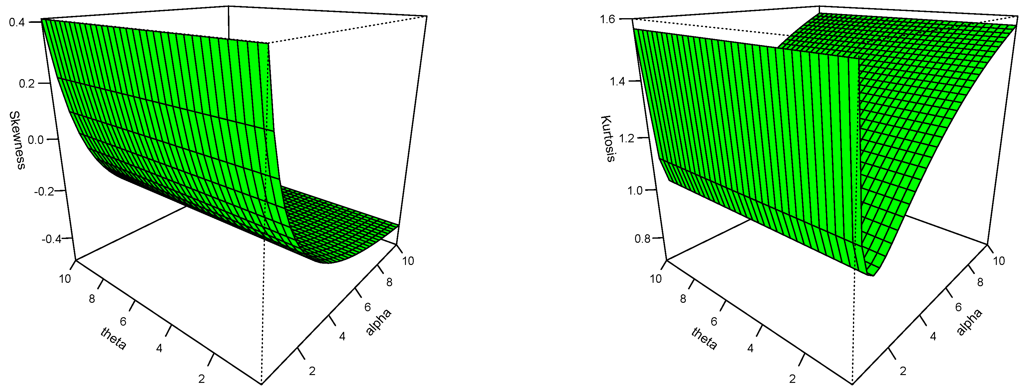
This section discusses some statistical properties and functions of the GPUD distribution.

2.2.1. Moments

If we have a random variable that we refer to as $X\sim$ that follows the GPUD(a,b,k) then the $r\mathrm{th}$ ordinary moment $\left({\mu }_k^r\right)$ of X can be calculated as follows:

$${\mu }_x^r=E_k\left[x^r\right]={\int }_{-\infty }^{\infty }{x}^r{f}_{X^k}\left(x\right)dx={\displaystyle \frac{M_{k+r}(a,b)}{M_k(a,b)}}.$$

(8)

In the case of the usual uniform distribution $k=0$, when $a=0$ and $b=1$, the $r\mathrm{th}$ moment is expressed as

$${\mu }_x^r(0,1)={\displaystyle \frac{M_{k+r}(0,1)}{M_k(0,1)}}={\displaystyle \frac{k+1}{k+r+1}}.$$

(9)

For the general case, in the interval $[a,b]$,

$${\mu }_x^r(a,b)={\displaystyle \frac{b^{k+r+1}-a^{k+r+1}}{(b-a)M_k(a,b)(k+r+1)}}.$$

(10)

The average and corresponding variance can be calculated by considering the previous result (Equation (10)):

$${\mu }_x^r(0,1)=E_k\left[x^r\right]={\displaystyle \frac{M_{k+r}(a,b)}{M_k(a,b)}}.$$

(11)

$${\sigma }_k^2(a,b)={\mu }_k^2(a,b)-{\left[{\mu }_k(a,b)\right]}^2={\displaystyle \frac{M_{k+2}(a,b)}{M_k(a,b)}}-{\left[{\displaystyle \frac{M_{k+1}(a,b)}{M_k(a,b)}}\right]}^2.$$

(12)

Similarly, the skewness and kurtosis coefficients are expressed through Equations (13) and (14), respectively:

$$\begin{array}{c}{\gamma }_{3_k}(a,b)=E_k\left[{\left({\displaystyle \frac{x-\mu }{\sigma }}\right)}^3\right]=\\ {\displaystyle \frac{1}{{\sigma }_k^3}}\left[E_k\left(x^3\right)-3\left[E_k\left(x\right)\right]E_k\left(x^2\right)+2{\left(E_k\left(x\right)\right)}^3\right].\end{array}$$

(13)

$$\begin{array}{c}{\gamma }_{4_k}(a,b)=E_k\left[{\left({\displaystyle \frac{x-\mu }{\sigma }}\right)}^4\right]=\\ {\displaystyle \frac{1}{{\sigma }_k^4}}\left[E_k\left(x^4\right)-4\left[E_k\left(x\right)\right]E_k\left(x^3\right)+6{\left[E_k\left(x\right)\right]}^3{E}_k\left(x^2\right)-3{\left[E_k\left(x\right)\right]}^4\right].\end{array}$$

(14)

Table 1. Mean, variance, coefficients of skewness, and kurtosis for GPUD.

$(\mathit{a},\mathit{b},\mathit{k})$	${\mathit{\mu }}_{\mathit{k}}$	${\mathit{\sigma }}_{\mathit{k}}^2$	${\mathit{\gamma }}_{3_{\mathit{k}}}$	${\mathit{\gamma }}_{4_{\mathit{k}}}$
$(2,5,0)$	3.5	0.75	0	−1.2
$(2,5,1)$	3.71	0.70	−0.29	−1.05
$(2,5,2)$	3.90	0.62	−0.55	−0.70
$(2,5,3)$	4.06	0.52	−0.79	−0.21
$(2,5,4)$	4.19	0.43	−0.98	0.34
$(2,5,5)$	4.29	0.35	−1.14	0.92

shows the corresponding calculations for the mean (${\mu }_k$), variance (${\sigma }_k^2$), skewness (${\gamma }_{3_k}$), and kurtosis (${\gamma }_{4_k}$) for $a=2$, $b=5$, and different values of k. In the case of the mean, each time the value of k increases, the ${\mu }_k$ approaches the value of parameter b. On the other hand, the variance decreases as the value of k increases; that is, the data becomes increasingly centered around the mean. Another aspect that can be observed with the data in Table 1 is the asymmetry compartment: when $k=0$, it can be said that the GPUD distribution is symmetric; however, when the value of k increases, the asymmetry coefficient turns out to be negative, which indicates that the distribution is skewed to the right. Likewise, the GPUD has a very low (negative) kurtosis for a value of $k=0$, which means that it has thin tails and produces fewer outliers. But, when the value of k increases, the kurtosis coefficient tends to be positive, indicating that the GPUD tends to have a relatively high distribution or show a higher peak.

2.2.2. Quantile Function and Random Number Generation

In probability and statistics, the Quantile Function (QF) has several uses, both in theory and in applications; in addition, the QF is associated with the CDF. In this sense, the Quantile Function of the GPUD is obtained by inverting Equation (3). First, a random number q is generated from the uniform distribution in the interval $(0,1)$, i.e., from $q\sim U(0,1)$. Second, the generalized inverse of the CDF (Equation (3)) is solved—that is, $F_{X^k}^{-1}\left(q\right)$. Finally, $x_q=F_{X^k}^{-1}\left(q\right)$ is calculated; this random variable $x_q$ has a behavior like the GPUD distribution—that is, $F_{X^k}$:

$$x_q={(a^{k+1}+(b^{k+1}-a^{k+1})q)}^{1/(k+1)}.$$

(15)

By setting $q=0.25$, $0.5$, and $0.75$ in Equation (15), the first, second, and third quartiles of the GPUD distribution can be obtained.

Table 2. Median GPUD distribution.

a	b	k	Median
2	5	0	3.5
2	5	1	3.80
2	5	2	4.05
2	5	3	4.23
2	5	4	4.36
2	5	5	4.45

presents the calculations of the median of the GPUD distribution for $a=2$, $b=5$, and different values of k. As seen in the table, when the value of parameter k increases, the value of the median tends to approach the value of parameter b. For example, when $k=0$, the median coincides with the value of ${\mu }_k$. However, when $k\ge 1$, the central value of the data shifts to the right.

3. Generalization of the Distribution of Jose and Krishna Using the GPUD Approach

To show the flexibility of the GPUD approach to modeling different statistical applications and performing data analysis, we generalized the model obtained by Jose and Krishna [18], called the Marshall–Olkin Extended Uniform (MOEU) distribution. The authors introduced a parameter $\theta >0$ into their model in the uniform distribution, now expressed as $U(0,\theta )$, where they considered the Survival Function as $\overline{F}\left(x\right)=1-(x/\theta )$, which is associated with a new distribution denoted as MOEU$(\alpha ,\theta )$.

So, the Survival Function of Jose and Krishna is expressed as

$$\overline{G}(x;\alpha ,\theta )={\displaystyle \frac{\alpha (\theta -x)}{\alpha \theta +(1-\alpha )x}},0<x<\theta ,\alpha >0,$$

(16)

where $\alpha$ is a shape parameter, $\theta$ is a scale parameter, and the Survival Function $\overline{G}=1-G$. Therefore, the CDF corresponding to the MOEU is

$$G(x;\alpha ,\theta )={\displaystyle \frac{x}{\alpha \theta +(1-\alpha )x}},0<x<\theta ,\alpha >0.$$

(17)

In turn, the PDF of the corresponding MOEU is given by

$$g(x;\alpha ,\theta )={\displaystyle \frac{\alpha \theta }{{\left[\alpha \theta +(1-\alpha )x\right]}^2}}0<x<\theta ,\alpha >0.$$

(18)

We have previously carried out the generalization of the model of Jayakumar and Sankaran [21] based on our GPUD approach; we show the corresponding generalization of Jose and Krishna [18] under the starting consideration that ${\overline{F}}_{X^k}\left(x\right)=1-x^k$, where $k=1,2,\dots ,n$. So, now we propose the Survival Function as ${\overline{F}}_{X^k}\left(x\right)=1-{(x/\theta )}^k$, where the CDF is $F_{X^k}\left(x\right)={(x/\theta )}^k$, with $0<x<\theta$, and where the new PDF is $f_{X^k}=F_{X^k}^{\prime }\left(x\right)={\displaystyle \frac{k}{{\theta }^k}}{x}^{k-1}$, with $\theta >k$. It is essential to mention that changing the variable from $(x/\theta )$ to ${(x/\theta )}^k$ expands the distribution family, allowing the modeling of different applications by introducing a new parameter.

Thus, our generalization is now expressed as an MOE-Powered Uniform distribution (MOE-PU), depending on the variables $(\alpha ,\theta ,k)$. Now, the new Survival Function is expressed as

$$\overline{G}(x;\alpha ,\theta ,k)={\displaystyle \frac{\alpha ({\theta }^k-x^k)}{\alpha {\theta }^k+(1-\alpha )x^k}},\theta >k,0<\alpha ,k=1,2,\dots ,n,$$

(19)

where $0<x<\theta$; the corresponding CDF is

$$G(x;\alpha ,\theta ,k)={\displaystyle \frac{x^k}{\alpha {\theta }^k+(1-\alpha )x^k}},$$

(20)

in such a way that the PDF is given by

$$g(x;\alpha ,\theta ,k)={\displaystyle \frac{k\alpha {\theta }^k{x}^{k-1}}{{\left[\alpha {\theta }^k+(1-\alpha )x^k\right]}^2}}.$$

(21)

It is essential to emphasize the nature of the decreasing function of the PDF of the MOE-PU. When $\alpha \in (0,1)$, the form of the PDF is a decreasing function on the interval $(0,\theta )$; if $k=1$ is considered, we will arrive at the same result as Jose and Krishna [18], with $g(0,\alpha ,\theta )=1/\left(\alpha \theta \right)$ and $g(\theta ,\alpha ,\theta )=\alpha /\theta$. On the other hand, if $\alpha >1$ then the PDF of the MOE-PU is an increasing function in $(0,\theta )$, with $g(0,\alpha ,\theta )=1/\left(\alpha \theta \right)$ and $g(\theta ,\alpha ,\theta )=\alpha /\theta$ (see Figure 3a).

From our generalization of the MOE-PU, when $k\ge 2$, we have $g(0,\alpha ,\theta ,k)=1/\left(\alpha \theta \right)$ and $g(\theta ,\alpha ,\theta ,k)=k\alpha /\theta$, so that the PDF is not necessarily monotonic for $\alpha \in (0,1)$ but is still increasing for $\alpha >1$ (see Figure 3b).

Figure 4a shows the CDF plot of the MOE-PU distribution for different values of k, considering a fixed value for $\alpha$ and $\theta$. In Figure 4b, the values of $\alpha$ change and the parameters k and $\theta$ remain fixed.

Figure 3 and Figure 4 show that the MOE-PU distribution has excellent advantages, since it can take several forms, allowing different data behaviors to be modeled.

3.1. Survival Function and Hazard Function of the MOE-PU

Let X be a continuous random variable whose CDF is $G(x;\alpha ,\theta ,k)$, Equation (20). Thus, the Survival Function (reliability function) of the MOE-PU distribution is described by

$$S(x;\alpha ,\theta ,k)=1-{\displaystyle \frac{x^k}{\alpha {\theta }^k+(1-\alpha )x^k}}.$$

(22)

The shape of the Survival Function of the MOE-PU is shown in Figure 5. In the context of reliability engineering, Figure 5a tells us that each time the value of parameter k increases, the probability that an element survives longer increases. On the other hand, Figure 5b shows that increasing the value of the shape parameter $\alpha$ increases the probability that a component survives longer. Furthermore, it can be inferred that at small values of k and $\alpha$, there is little reliability that an element will survive over time.

On the other hand, the Hazard Function, often called the failure rate, can be considered a random variable, in terms of time. For example, in reliability engineering, the HF describes the probability that a failure will occur in a component or system at time t, given that the failure did not occur until that moment. In this sense, the HF of the MOE-PU is described as

$$h(x;\alpha ,\theta ,k)={\displaystyle \frac{g(x;\alpha ,\theta ,k)}{S(x;\alpha ,\theta ,k)}},$$

(23)

using Equations (21) and (22) in Equation (23). The HF of the MOE-PU can be expressed as

$$h(x;\alpha ,\theta ,k)={\displaystyle \frac{k{x}^{k-1}{\theta }^k}{\left[\alpha {\theta }^k+(1-\alpha )x^k\right]({\theta }^k-x^k)}},$$

(24)

When $k=1$, the result reported in the model was obtained by Jose and Krishna [18]:

$$\begin{array}{c}h(x;\alpha ,\theta ,1)={\displaystyle \frac{\theta }{\left[\alpha \theta +(1-\alpha )x\right](\theta -x)}}.\end{array}$$

Figure 6 presents the shape of the HF of the MOE-PU for different parameter values. As shown in Figure 6, the MOE-PU distribution can model failure times where the behavior can be monotonic or non-monotonic, like those of a bathtub curve. For example, in Figure 6a, when k = 0, the shape of the failure function is typical of a bathtub, where the flat line at the bottom represents the service life. The longer that flat line is, the longer the lifetime the MOE-PU distribution can model. The proposed approach of incorporating the shape parameter k allows for the flexibility of modeling the failure times of both bathtub curves and unimodal failure curves, as shown in Figure 6a,b:

3.2. Quantile Function of the MOE-PU

In the case of the MOE-PU distribution, its Quantile Function can be obtained by inverting the CDF in Equation (20), which takes the form:

$$X_q=\sqrt[k]{{\displaystyle \frac{\alpha {\theta }^{k}q}{1-(1-\alpha )q}}},$$

(25)

where q follows a uniform distribution (0, 1) to generate random numbers; the MOE-PU distribution’s first, second, and third quantiles can be calculated by substituting $q=0.25$, $0.5$, and $0.75$, respectively, into Equation (25).

Furthermore, we can derive the skewness and kurtosis measures of the MOE-PU distribution from Equation (25), considering the following two models:

$$SK(\alpha ,\theta ,k)={\displaystyle \frac{Q(3/4)+Q(1/4)-2Q(1/2)}{Q(3/4)-Q(1/4)}},$$

(26)

$$KU(\alpha ,\theta ,k)={\displaystyle \frac{Q(7/8)+Q(3/8)-Q(5/8)-Q(1/8)}{Q(6/8)-Q(2/8)}}.$$

(27)

To investigate and analyze the skewness and kurtosis compartment of the MOE-PU distribution when $k=1$ and the parameters $\alpha$ and $\theta$ take different values, Figure 7 is shown in 3D. The analysis of the graphs shows that the two parameters are effective in the variation of skewness and kurtosis. In the case of the asymmetry coefficient, both negative and positive values are obtained; that is, the MOE-PU distribution can be skewed to the right and the left, in addition to being symmetric in some combination of the parameters $\alpha$ and $\theta$. For the kurtosis coefficient, the MOE-PU distribution presents positive values when $k=1$, which means that the distribution will present heavier tails and a more pronounced peak.

3.3. Maximum Likelihood Estimators of the MOE-PU

The Maximum Likelihood Estimator method is the most-used method in statistical inference for parameter estimation, since it provides complete information about the unknown parameters of a distribution. Suppose that $x_1,x_2,\dots ,x_n$ is a random sample of size n of the MOE-PU distribution with the PDF (Equation (21)), such that the log-likelihood function is specified by

$$L(x;\alpha ,\theta ,k)=\prod _{i=1}^{n}g(x_i;\alpha ,\theta ,k).$$

(28)

From our proposal, the log-likelihood function is expressed as

$$logL(x;\alpha ,\theta ,k)=log\prod _{i=1}^{n}g(x_i;\alpha ,\theta ,k)=\sum _{i=1}^{n}log\left[{\displaystyle \frac{k\alpha {\theta }^k{x}_i^{k-1}}{{\left(\alpha {\theta }^k+(1-\alpha )x^k\right)}^2}}\right].$$

(29)

The maximum likelihood function can be estimated as

$$\begin{array}{c}logL(x;\alpha ,\theta ,k)=nlog\left(k\right)+nlog\left(\alpha \right)+nklog\left(\theta \right)+\\ (k-1){\displaystyle \sum _{i=1}^n}log\left(x_i\right)-2{\displaystyle \sum _{i=1}^n}log\left[\alpha {\theta }^k+(1-\alpha )x_i^k\right].\end{array}$$

(30)

To calculate the estimators of the unknown parameters, as well as obtaining the covariance matrix $I^{-1}\left(\beta \right)$, the partial derivations of the log-likelihood function must be calculated, which are

$${\displaystyle \frac{\partial logL}{\partial \alpha }}={\displaystyle \frac{n}{\alpha }}-2\sum _{i=1}^n{\displaystyle \frac{{\theta }^k-x_i^k}{\alpha {\theta }^k+(1-\alpha )x_i^k}},$$

(31)

$${\displaystyle \frac{\partial logL}{\partial \theta }}={\displaystyle \frac{kn}{\theta }}-2\sum _{i=1}^n{\displaystyle \frac{\alpha k{\theta }^{k-1}}{\alpha {\theta }^k+(1-\alpha )x_i^k}},$$

(32)

$${\displaystyle \frac{\partial logL}{\partial k}}={\displaystyle \frac{n}{k}}+nlog\left(\theta \right)+\sum _{i=1}^{n}log\left(x_i\right)-2\sum _{i=1}^n{\displaystyle \frac{\alpha {\theta }^{k}log\left(\theta \right)+x_i^{k}log\left(x_i\right)(1-\alpha )}{\alpha {\theta }^k+(1-\alpha )x_i^k}}.$$

(33)

Furthermore, the second partial derivatives of the MOE-PU distribution concerning the parameters $\alpha$, $\theta$, and k are expressed as

$${\displaystyle \frac{{\partial }^{2}logL}{\partial {\alpha }^2}}=-{\displaystyle \frac{n}{{\alpha }^2}}+2\sum _{i=1}^n{\displaystyle \frac{{\left({\theta }^k-x_i^k\right)}^2}{{\left[\alpha {\theta }^k+(1-\alpha )x_i^k\right]}^2}},$$

(34)

$${\displaystyle \frac{{\partial }^{2}logL}{\partial {\theta }^2}}=-{\displaystyle \frac{kn}{{\theta }^2}}-2\sum _{i=1}^n{\displaystyle \frac{\alpha k(k-1){\theta }^{k-2}\left[\alpha {\theta }^k+(1-\alpha )x_i^k\right]-{\alpha }^2{k}^2{\theta }^{2k-2}}{{\left[\alpha {\theta }^k+(1-\alpha )x_i^k\right]}^2}},$$

(35)

$${\displaystyle \frac{{\partial }^{2}logL}{\partial k^2}}=-{\displaystyle \frac{n}{k^2}}-2\sum _{i=1}^n{\displaystyle \frac{A\left[\left(\alpha {\theta }^k+(1-\alpha )x_i^k\right)-\left(x_i^k(1-\alpha )log\left(x_i\right)\right)\right]}{{\left[\alpha {\theta }^k+(1-\alpha )x_i^k\right]}^2}},$$

(36)

$$\begin{array}{c}A=\left[\alpha {\left(log\left(\theta \right)\right)}^2{\theta }^k+(1-\alpha )x_i^k{\left(log\left(x_i\right)\right)}^2\right],\end{array}$$

$${\displaystyle \frac{{\partial }^{2}logL}{\partial \alpha \partial \theta }}=-2\sum _{i=1}^n{\displaystyle \frac{x_i^{k}k{\theta }^{k-2}}{{\left[\alpha {\theta }^k-x_i^k(-1+\alpha )\right]}^2}},$$

(37)

$${\displaystyle \frac{{\partial }^{2}logL}{\partial \alpha \partial k}}=\sum _{i=1}^n{\displaystyle \frac{-2{\theta }^k{x}_i^k\left(log\left(\theta \right)-log\left(x_i\right)\right)}{{\left[\alpha {\theta }^k+(1-\alpha )x_i^k\right]}^2}},$$

(38)

$${\displaystyle \frac{{\partial }^{2}logL}{\partial \theta \partial k}}=\sum _{i=1}^n\left({\displaystyle \frac{2\alpha {\theta }^{k-1}\left(-\alpha {\theta }^k+(-1+\alpha )(k(log\left(\theta \right)-log\left(x_i\right))+1)x_i^k\right)}{{\left[\alpha {\theta }^k-x_i^k(-1+\alpha )\right]}^2}}\right)+{\displaystyle \frac{n}{\theta }}.$$

(39)

4. MOE-PU Monte Carlo Simulation Study

This section addresses a Monte Carlo simulation study to evaluate the performance of the Maximum Likelihood Estimator (MLE) method, considering different values of the parameters of the MOE-PU model and different sample sizes n. The simulation was replicated 1000 times with four different sample sizes, $n=50,100,150$, and 200, and four alternative scenarios were considered, whose parameter combinations were as follows: I: $\alpha =0.009$, $\theta =10$, $k=2$; II: $\alpha =0.004$, $\theta =6$, $k=3$; III: $\alpha =3.5$, $\theta =56$, $k=1$; IV: $\alpha =0.1$, $\theta =25$, $k=4$. To generate the random sample of the MOE-PU, Equation (25) was used. It should be remembered that q is a uniform random number (0,1). In order to analyze the performance of the Maximum Likelihood Estimator, the following statistics were calculated: the Average Values of Estimates (AVE), the associated average Mean Squared Error (MSE), the average Mean Relative Estimates (MREs), and the average values of absolute bias (Bias). These statistics were defined for a specific parameter $\varphi$, which was estimated by $\widehat{\varphi }$, as shown below:

$$\begin{array}{c}\mathrm{AVE}={\displaystyle \frac{1}{N}}\sum _{i=1}^N{\widehat{\varphi }}_i,\mathrm{MSE}={\displaystyle \frac{1}{N}}\sum _{i=1}^N{\left({\widehat{\varphi }}_i-\varphi \right)}^2,\\ \mathrm{MREs}={\displaystyle \frac{1}{N}}\sum _{i=1}^N{\displaystyle \frac{\left|{\widehat{\varphi }}_i-\varphi \right|}{\varphi }},\mathrm{Bias}={\displaystyle \frac{1}{N}}\sum _{i=1}^N\left|{\widehat{\varphi }}_i-\varphi \right|,\end{array}$$

where $\varphi =\alpha$, $\theta$ or k and ${\widehat{\varphi }}_i(i=1,2,\dots ,N)$ were simulated estimates of $\varphi$. The Monte Carlo simulation algorithm is presented below:

Step 1

First, the values of the parameters $\alpha$, $\theta$, and k are defined for each simulation. The sample size $n=50,100,150$, and 200 is also defined, as well as the number of simulations $N=1000$;

Step 2

Generate a random sample q following the uniform distribution $(0,1)$ of size $n=50,100,150$, and 200, respectively;

Step 3

Generate a random sample $X_q$ following the MOE-PU distribution from Equation (25) for $n=50,100,150$, and 200, respectively;

Step 4

Each random sample from Step 3 is simulated N times, and the estimate of the parameters $\alpha$, $\theta$, and k, as well as the values of the AVE, MSE, MREs, and Bias, are calculated;

Step 5

The required results are obtained, based on the different combinations of the model parameters, which are shown in Table 3, Table 4, Table 5 and Table 6;

Step 6

Analyzing Table 3, Table 4, Table 5 and Table 6 reveals that there is a gradual decrease in Bias with increasing sample size.

Considering the previous algorithm, Table 3, Table 4, Table 5 and Table 6 show the results of estimating the parameters of the MOE-PU model obtained in the simulation. The AVE, MSE, MREs, and Bias calculations are also included. These findings indicate that the estimates are reliable and very precise for the values of the genuine parameters; that is, the calculations obtained in the Maximum Likelihood Estimator method are reliable (Equations (30)–(39)). Furthermore, the MSE and Bias decreased in all scenarios as the sample size increased.

Table 3. Monte Carlo simulation results for $(\alpha =0.009,\theta =10,k=2)$.

n	Parameter	AVE	MSE	MREs	Bias
50	$\alpha$	0.0092	5.068 × 10−6	0.1961	0.0017
	$\theta$	9.9883	3.842 × 10−8	1.169 × 10−6	1.169 × 10−6
	k	1.9937	9.715 × 10−6	8.065 × 10−5	0.0001
100	$\alpha$	0.0091	2.623 × 10−6	0.1403	0.0012
	$\theta$	10.010	8.049 × 10−8	1.622 × 10−6	1.622 × 10−6
	k	2.0004	3.614 × 10−6	6.689 × 10−5	0.0001
150	$\alpha$	0.0091	1.843 × 10−6	0.1150	0.0010
	$\theta$	10.006	2.128 × 10−9	5.215 × 10−7	5.215 × 10−7
	k	2.0002	1.843 × 10−7	2.703 × 10−5	5.406 × 10−5
200	$\alpha$	0.0091	1.447 × 10−6	0.1025	0.0009
	$\theta$	10.002	1.125 × 10−7	4.168 × 10−7	4.168 × 10−6
	k	2.0003	4.165 × 10−7	2.408 × 10−5	4.807 × 10−5

Table 3. Monte Carlo simulation results for $(\alpha =0.009,\theta =10,k=2)$.

n	Parameter	AVE	MSE	MREs	Bias
50	$\alpha$	0.0092	5.068 × 10−6	0.1961	0.0017
	$\theta$	9.9883	3.842 × 10−8	1.169 × 10−6	1.169 × 10−6
	k	1.9937	9.715 × 10−6	8.065 × 10−5	0.0001
100	$\alpha$	0.0091	2.623 × 10−6	0.1403	0.0012
	$\theta$	10.010	8.049 × 10−8	1.622 × 10−6	1.622 × 10−6
	k	2.0004	3.614 × 10−6	6.689 × 10−5	0.0001
150	$\alpha$	0.0091	1.843 × 10−6	0.1150	0.0010
	$\theta$	10.006	2.128 × 10−9	5.215 × 10−7	5.215 × 10−7
	k	2.0002	1.843 × 10−7	2.703 × 10−5	5.406 × 10−5
200	$\alpha$	0.0091	1.447 × 10−6	0.1025	0.0009
	$\theta$	10.002	1.125 × 10−7	4.168 × 10−7	4.168 × 10−6
	k	2.0003	4.165 × 10−7	2.408 × 10−5	4.807 × 10−5

Table 4. Monte Carlo simulation results for $(\alpha =0.004,\theta =6,k=3)$.

n	Parameter	AVE	MSE	MREs	Bias
50	$\alpha$	0.0077	1.825 × 10−5	0.9597	0.0038
	$\theta$	5.8000	0.0399	0.0333	0.1999
	k	2.7000	0.0899	0.0999	0.2999
100	$\alpha$	0.0053	2.801 × 10−6	0.3530	0.0014
	$\theta$	5.8000	0.0399	0.0333	0.1999
	k	2.9000	0.0099	0.0333	0.0999
150	$\alpha$	0.0054	2.605 × 10−6	0.3596	0.0014
	$\theta$	5.8000	0.0399	0.0333	0.1999
	k	2.9000	0.0099	0.0333	0.0999
200	$\alpha$	0.0041	2.150 × 10−7	0.0892	0.0003
	$\theta$	5.9999	1.634 × 10−8	1.313 × 10−6	7.878 × 10−6
	k	2.9999	3.041 × 10−7	1.043 × 10−5	3.131 × 10−5

Table 4. Monte Carlo simulation results for $(\alpha =0.004,\theta =6,k=3)$.

n	Parameter	AVE	MSE	MREs	Bias
50	$\alpha$	0.0077	1.825 × 10−5	0.9597	0.0038
	$\theta$	5.8000	0.0399	0.0333	0.1999
	k	2.7000	0.0899	0.0999	0.2999
100	$\alpha$	0.0053	2.801 × 10−6	0.3530	0.0014
	$\theta$	5.8000	0.0399	0.0333	0.1999
	k	2.9000	0.0099	0.0333	0.0999
150	$\alpha$	0.0054	2.605 × 10−6	0.3596	0.0014
	$\theta$	5.8000	0.0399	0.0333	0.1999
	k	2.9000	0.0099	0.0333	0.0999
200	$\alpha$	0.0041	2.150 × 10−7	0.0892	0.0003
	$\theta$	5.9999	1.634 × 10−8	1.313 × 10−6	7.878 × 10−6
	k	2.9999	3.041 × 10−7	1.043 × 10−5	3.131 × 10−5

Table 5. Monte Carlo simulation results for $(\alpha =3.5,\theta =56,k=1)$.

n	Parameter	AVE	MSE	MREs	Bias
50	$\alpha$	3.3775	0.0191	0.0351	0.1229
	$\theta$	56.963	0.9445	0.0172	0.9686
	k	0.9510	0.0351	0.1491	0.1491
100	$\alpha$	3.4142	0.0111	0.0245	0.0858
	$\theta$	56.941	0.9008	0.0168	0.9435
	k	0.9207	0.0218	0.1217	0.1217
150	$\alpha$	3.4404	0.0063	0.0170	0.0598
	$\theta$	56.924	0.8730	0.0165	0.9279
	k	0.9081	0.0187	0.1154	0.1154
200	$\alpha$	3.5152	0.0014	0.0066	0.0233
	$\theta$	56.002	0.0044	0.0003	0.0207
	k	1.0025	0.0099	0.0784	0.0784

Table 5. Monte Carlo simulation results for $(\alpha =3.5,\theta =56,k=1)$.

n	Parameter	AVE	MSE	MREs	Bias
50	$\alpha$	3.3775	0.0191	0.0351	0.1229
	$\theta$	56.963	0.9445	0.0172	0.9686
	k	0.9510	0.0351	0.1491	0.1491
100	$\alpha$	3.4142	0.0111	0.0245	0.0858
	$\theta$	56.941	0.9008	0.0168	0.9435
	k	0.9207	0.0218	0.1217	0.1217
150	$\alpha$	3.4404	0.0063	0.0170	0.0598
	$\theta$	56.924	0.8730	0.0165	0.9279
	k	0.9081	0.0187	0.1154	0.1154
200	$\alpha$	3.5152	0.0014	0.0066	0.0233
	$\theta$	56.002	0.0044	0.0003	0.0207
	k	1.0025	0.0099	0.0784	0.0784

Table 6. Monte Carlo simulation results for $(\alpha =0.1,\theta =25,k=4)$.

n	Parameter	AVE	MSE	MREs	Bias
50	$\alpha$	0.1254	0.0018	0.3180	0.0318
	$\theta$	24.001	0.9977	0.0399	0.9987
	k	3.9958	0.0029	0.0015	0.0061
100	$\alpha$	0.1119	0.0005	0.1845	0.0184
	$\theta$	24.499	0.2500	0.0200	0.5001
	k	3.9983	0.0009	0.0006	0.0027
150	$\alpha$	0.1043	0.0002	0.1197	0.1197
	$\theta$	24.799	0.0400	0.0080	0.2000
	k	3.9995	1.739 × 10−6	0.0002	0.0009
200	$\alpha$	0.1009	0.0001	0.0999	0.0099
	$\theta$	25.000	1.053 × 10−6	9.522 × 10−6	0.0002
	k	3.9997	0.0001	0.0002	0.0011

Table 6. Monte Carlo simulation results for $(\alpha =0.1,\theta =25,k=4)$.

n	Parameter	AVE	MSE	MREs	Bias
50	$\alpha$	0.1254	0.0018	0.3180	0.0318
	$\theta$	24.001	0.9977	0.0399	0.9987
	k	3.9958	0.0029	0.0015	0.0061
100	$\alpha$	0.1119	0.0005	0.1845	0.0184
	$\theta$	24.499	0.2500	0.0200	0.5001
	k	3.9983	0.0009	0.0006	0.0027
150	$\alpha$	0.1043	0.0002	0.1197	0.1197
	$\theta$	24.799	0.0400	0.0080	0.2000
	k	3.9995	1.739 × 10−6	0.0002	0.0009
200	$\alpha$	0.1009	0.0001	0.0999	0.0099
	$\theta$	25.000	1.053 × 10−6	9.522 × 10−6	0.0002
	k	3.9997	0.0001	0.0002	0.0011

5. Application to Real Data

In this Section, three case studies dedicated to reliability analysis are presented, where the MOE-PU was tested and compared with other distributions. For this, the following was considered:

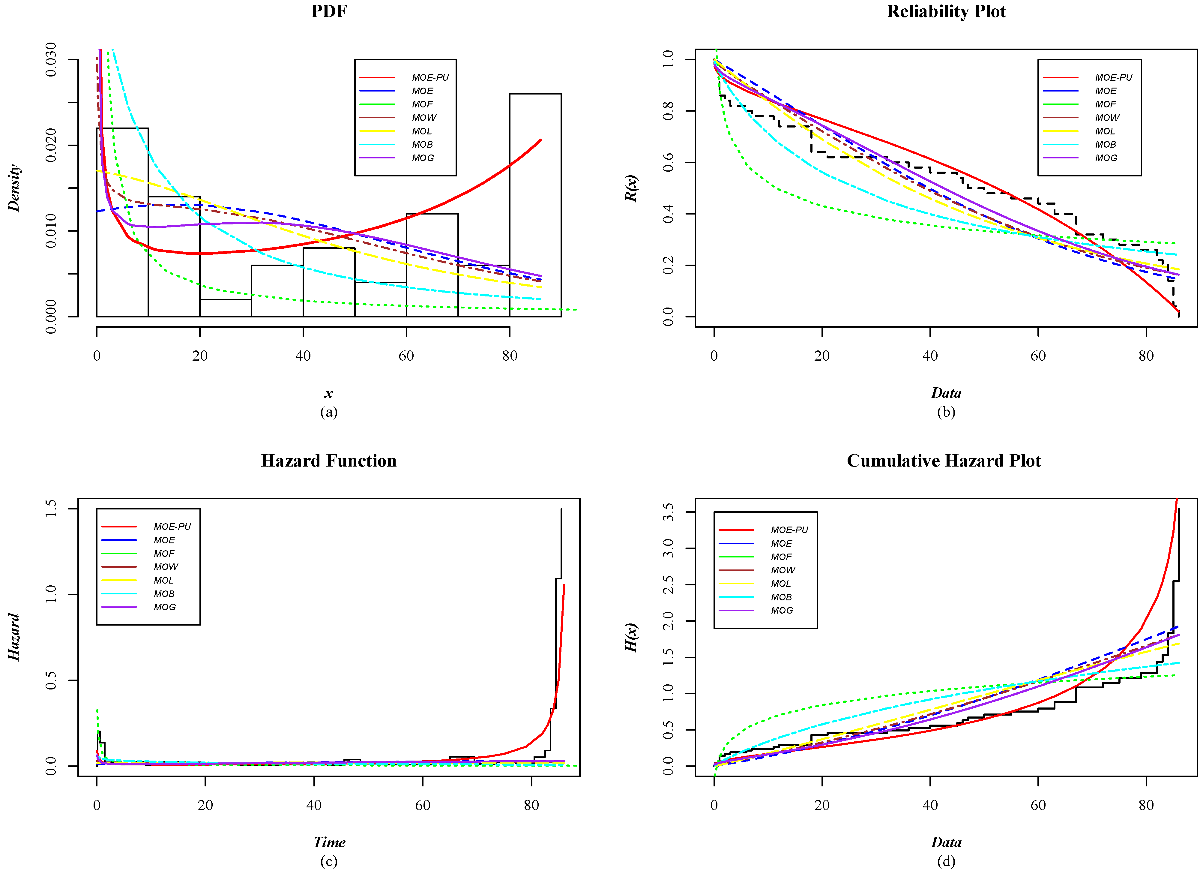
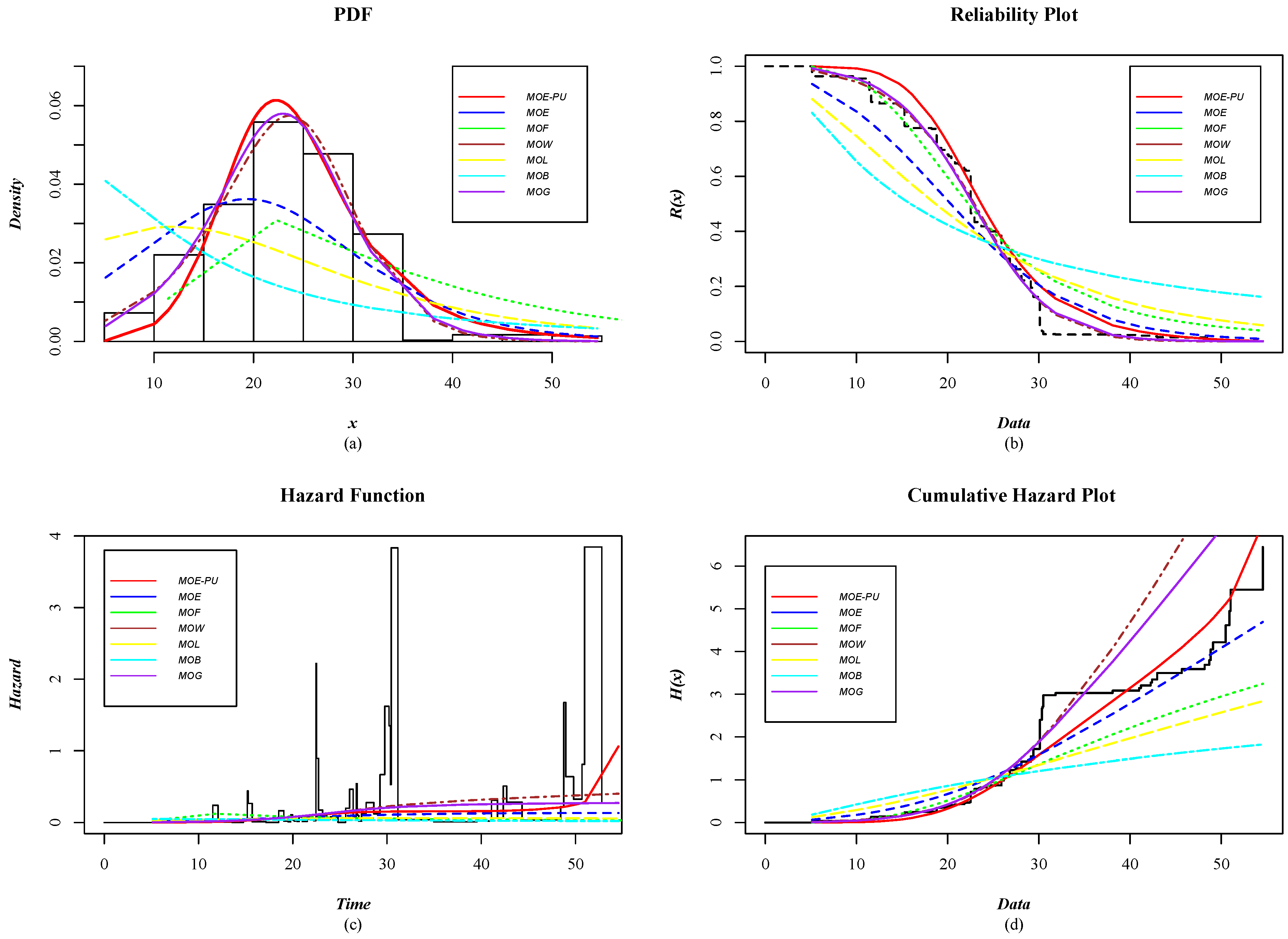
• The distributions considered were developed from the approach of Marshall and Olkin [19], as follows: Marshall–Olkin Exponential (MOE); Marshall–Olkin–Frechet (MOF); Marshall–Olkin–Weibull (MOW); Marshall–Olkin–Lomax (MOL); Marshall–Olkin–Burr XII (MOB); and Marshall–Olkin–Gamma (MOG). For more details of the distributions mentioned above, see Nadarajah and Rocha [22].

  Table 7. PDF of the models used for the case studies.

  Statistical Distribution	$\mathit{g}\left(\mathit{x}\right)$
  MOE	${\displaystyle \frac{\beta \lambda e^{-\lambda x}}{{\left(1-(1-\beta )e^{-\lambda x}\right)}^2}}$
  MOF	${\displaystyle \frac{\beta \left(\theta \left(\frac{1}{\gamma }\right)e^{-{(x/\gamma )}^{-\theta }}{\left(\frac{x}{\gamma }\right)}^{-\theta -1}\right)}{\beta +(1-\beta )e^{-{(x/\gamma )}^{-\theta }}}}$
  MOW	${\displaystyle \frac{\beta \left(\left(\frac{\alpha }{\lambda }\right){\left(\frac{x}{\lambda }\right)}^{\alpha -1}{e}^{-{(x/\lambda )}^{\alpha }}\right)}{{\left(\beta +(1-\beta )\left(1-e^{-{(x/\lambda )}^{\alpha }}\right)\right)}^2}}$
  MOL	${\displaystyle \frac{\beta \left(\frac{\theta \gamma }{{\left(1+\theta x\right)}^{\gamma +1}}\right)}{{\left(\beta +\left(1-\beta \right){\left(1-(1+\theta x\right)}^{-\gamma }\right)}^2}}$
  MOB	${\displaystyle \frac{\beta \left(\delta \theta {\left(1+x^{\delta }\right)}^{-\theta -1}{x}^{\delta -1}\right)}{{\left(\beta +(1-\beta )\left(1-{\left(1+x^{\delta }\right)}^{-\theta }\right)\right)}^2}}$
  MOG	${\displaystyle \frac{\beta \left(\frac{1}{{\delta }^{\theta }\mathsf{\Gamma }\left(\theta \right)}{x}^{\theta -1}{e}^{-x/\delta }\right)}{{\left(\beta +\left(1-\beta \right)\left(\frac{1}{\mathsf{\Gamma }\left(\theta \right)}\gamma \left(\theta ,\delta x\right)\right)\right)}^2}}$

  shows the density functions of the models used to analyze and compare the performance of the MOE-PU distribution against those models.
• To estimate the parameters of the distributions used in the comparative analysis, the open-source software “R” (version R-4.4.1) was used with the MaxLik library (version 1.5-2.1). It is worth mentioning that “R” is one of the environments most used by the scientific community for statistical analysis. The code used in R to estimate the parameters of the MOE-PU distribution is attached in Appendix A.
• In the three study cases, uncensored data were considered; all the information (all measurements) of the study variable was known.

5.1. Case Study 1: Reliability Analysis for Fatigue Times for 6061-T6 Aluminum Coupons

Reliability analysis applied to engineering is one of the most-used tools to determine the useful life of a material, product, or device, since this tool is the means to anticipate failures and know the probability that these will occur. In this sense, the first case study analyzed the fatigue times of 100 6061-T6 aluminum coupons cut parallel to the rolling direction and oscillated at 18 cycles per second. Fatigue testing allowed us to determine the useful life expected from a material subjected to cyclic loading. Fatigue times were reported by Birnbaum and Saunders [23], which are presented in

Table 8. Lifetimes in cycles × ${10}^{-3}$ for 100 specimens at maximum stress per cycle of 31,000 psi.

Lifetimes
70	90	96	97	99	100	103	104	104	105
107	108	108	108	109	109	112	112	113	114
114	114	116	119	120	120	120	121	121	123
124	124	124	124	124	128	128	129	129	130
130	130	131	131	131	131	131	132	132	132
133	134	134	134	134	134	136	136	137	138
138	138	139	139	141	141	142	142	142	142
142	142	144	144	145	146	148	148	149	151
151	152	155	156	157	157	157	157	158	159
162	163	163	164	166	166	168	170	174	196

:

In order to apply reliability engineering in this case study, the behavior of the data presented in Table 8 was first empirically verified. For this case, a TTT graph was used to analyze the shape of the failure function, as shown in Figure 8. It is important to remember that the primary purpose of this graph was to distinguish between an increasing Hazard Function, a decreasing Hazard Function, or a Hazard Function in the form of a bathtub curve. The dotted line was obtained in the following way: $i/n$, where $i=1,2,3,\dots ,n$; i represents the failure number; in the case of Figure 8, $n=100$. The blue curve was constructed in the following way: $T_{(i/n)}={\displaystyle \frac{{\sum }_{j=1}^i{T}_{(j:n)}+(n-i)T_{(i:n)}}{{\sum }_{j=1}^n{T}_{(j:n)}}}$, where $i=1,2,3,\dots ,n$, and $T_{(1:n)}=1,2,3,\dots ,n$. T represents the failure time. Concerning Figure 8, the graph results suggest that the data presented an increasing Hazard Function; that is, the aluminum coupons were likely to fail or deteriorate over time.

Table 9. Parameter estimates and goodness-of-fit statistics for case study 1.

Model	MLEs	logL	AIC	BIC	W*	A*	K-S	p-Value
MOE-PU	$\widehat{\alpha }=0.0153$	−446.21	898.42	906.23	0.0484	0.4135	0.0588	0.8788
	$\widehat{\theta }=196.005$
	$\widehat{k}=10.7003$
MOE	$\widehat{\beta }=4.9611$	−545.08	1094.16	1099.37	0.0513	0.3042	0.4439	7.77 × ${10}^{-16}$
	$\widehat{\lambda }=0.0173$
MOF	$\widehat{\beta }=35.056$	−459.81	925.62	933.44	0.1120	0.6530	0.1622	0.0103
	$\widehat{\theta }=7.1004$
	$\widehat{\gamma }=76.881$
MOW	$\widehat{\beta }=29.984$	−499.90	1005.81	1013.62	0.0449	0.2730	0.3623	7.88 × ${10}^{-12}$
	$\widehat{\alpha }=1.0708$
	$\widehat{\lambda }=35.466$
MOL	$\widehat{\beta }=2.8187$	−582.36	1170.72	1178.53	0.0708	0.4107	0.4267	3.33 × ${10}^{-16}$
	$\widehat{\theta }=0.0039$
	$\widehat{\gamma }=3.7093$
MOB	$\widehat{\beta }=28.663$	−653.78	1313.57	1321.39	0.1017	0.5829	0.5264	0.02 × ${10}^{-17}$
	$\widehat{\theta }=0.1854$
	$\widehat{\delta }=4.2177$
MOG	$\widehat{\beta }=21.913$	−457.11	920.22	928.04	0.0379	0.2552	0.1383	0.0435
	$\widehat{\theta }=7.3868$
	$\widehat{\delta }=0.0976$

shows the comparative analysis results for each distribution. To compare the performance of the MOE-PU distribution with the other distributions, in terms of goodness of fit, we used six tests or measures of goodness of fit, such as the Akaike Information Criterion (AIC), the Bayesian Information Criterion (BIC), Crammer-von Mises (W*), Anderson–Darling (A*), Kolmogorov–Smirnov (K-S), and the p-value (p) of K-S. Additionally, the table provides the MLEs, and the estimated maximum likelihood function (log L) was calculated. Generally, the model that presents the lowest goodness-of-fit statistics will be the distribution that best fits the data’s behavior. In this sense, the data in Table 9 show that the MOE-PU distribution presented the best results compared to the other distributions. It is worth mentioning that the MOW and MOG distributions presented the lowest values in W* and A*. However, there was no significant difference, since the MOE-PU distribution had the highest p-value. That is, the MOE-PU distribution better modeled the behavior of the data, so this model can be used to make decisions in reliability engineering studies.

Our reliability analysis, conducted with a comprehensive graphical approach, visualized the performance of the MOE-PU distribution in relation to the data presented in Table 8. For this analysis, the following graphs were used: PDF, Hazard Function, Cumulative Hazard Plot, and Reliability Plot, as shown in Figure 9; these graphs were meticulously obtained or calculated based on the parameter estimates reported in Table 9. This thorough analysis allows us to clearly see the performance of each of the distributions used for the reliability analysis.

First, our study focused on analyzing how each of the PDFs of the distributions used fitted the histogram of the data (fatigue times) (see Figure 9a). The graph results show that the proposed model (MOE-PU) offered a very competitive fit relating to the histogram, so it can be inferred that the new distribution more accurately exposes the actual behavior of fatigue times. This finding underscores a critical aspect for reliability engineering professionals, who play a decisive role in minimizing bias or loss of information in the analyzed data. Subsequently, the behavior of the data lifetimes was analyzed from the perspective of a reliability graph (see Figure 9b). The graph shows that the MOE-PU distribution was associated with more points regarding the empirical reliability of Kaplan–Meier compared to the other distributions analyzed.

Figure 9c shows how the failures or fatigue of 6061-T6 aluminum behaves in the different distributions; in other words, the figure shows the lifetimes. The results show that the MOE-PU represents an increasing hazard rate; the 6061-T6 aluminum coupons will present a failure or fatigue as time passes. Figure 9d shows a cumulative hazard plot, which confirms the coherence between the proposed model (MOE-PU) and the lifetimes established in this case. In conclusion, the MOE-PU distribution can be a good option for materials science engineers to determine reliability evaluation and analysis techniques that allow them to minimize the durability and reliability problems of materials due to their properties.

5.2. Case Study 2: Reliability Analysis for Bladder Cancer Data

In this second case, a reliability study was carried out related to remission times (in months) of patients with bladder cancer. The data used for the analysis were reported by Shakhatreh [24], where 128 data were considered.

Table 10. Remission times of patients with bladder cancer for case study 2.

Lifetimes
0.08	0.20	0.40	0.50	0.51	0.81	0.90	1.05	1.19	1.26
1.35	1.40	1.46	1.76	2.02	2.02	2.07	2.09	2.23	2.26
2.46	2.54	2.62	2.64	2.69	2.69	2.75	2.83	2.87	3.02
3.25	3.31	3.36	3.36	3.48	3.52	3.57	3.64	3.70	3.82
3.88	4.18	4.23	4.26	4.33	4.34	4.40	4.50	4.51	4.87
4.98	5.06	5.09	5.17	5.32	5.32	5.34	5.41	5.41	5.49
5.62	5.71	5.85	6.25	6.54	6.76	6.93	6.94	6.97	7.09
7.26	7.28	7.32	7.39	7.59	7.62	7.63	7.66	7.87	7.93
8.26	8.37	8.53	8.65	8.66	9.02	9.22	9.47	9.74	10.06
10.34	10.66	10.75	11.25	11.64	11.79	11.98	12.02	12.03	12.07
12.63	13.11	13.29	13.80	14.24	14.76	14.77	14.83	15.96	16.62
17.12	17.14	17.36	18.10	19.13	20.28	21.73	22.69	23.63	25.74
25.82	26.31	32.15	34.26	36.66	43.01	46.12	79.05

shows the behavior of the remission times of the patients who were under study.

Preliminary analysis of the cancer data shows that they came from a positively skewed distribution. Taking into account the same criteria as the previous case study, we began by empirically analyzing the behavior of the data in Table 10. A TTT graph was considered, to study the shape of the failure function, as shown in Figure 10. The plot shows that the empirical hazard rate function was unimodal (blue curve). That is, the data presented an upside-down bathtub Hazard Function. This meant that the riskiest period in the remission stage was in the initial period. But gradually, the remission stage stabilized as time passed; however, the short-term risk increased again.

Table 11. Parameter estimates and goodness-of-fit statistics for the remission time of case study 2.

Model	MLEs	logL	AIC	BIC	W*	A*	K-S	p-Value
MOE-PU	$\widehat{\alpha }=0.0087$	−410.46	826.92	835.47	0.0310	0.2441	0.0451	0.9565
	$\widehat{\theta }=104.5$
	$\widehat{k}=1.662$
MOE	$\widehat{\beta }=1.0711$	−414.32	832.65	838.36	0.1268	0.7591	0.0793	0.3955
	$\widehat{\lambda }=0.1101$
MOF	$\widehat{\beta }=15.357$	−425.48	856.97	865.52	0.2463	1.6384	0.1168	0.0607
	$\widehat{\theta }=1.2248$
	$\widehat{\gamma }=0.5530$
MOW	$\widehat{\beta }=1.0221$	−414.24	834.49	843.04	0.1339	0.8011	0.0771	0.4309
	$\widehat{\alpha }=1.0389$
	$\widehat{\lambda }=9.0471$
MOL	$\widehat{\beta }=4.3565$	−410.62	827.25	835.81	0.0577	0.3311	0.0497	0.9092
	$\widehat{\theta }=0.0816$
	$\widehat{\gamma }=3.9400$
MOB	$\widehat{\beta }=23.397$	−410.80	827.79	836.15	0.0310	0.2260	0.0527	0.8687
	$\widehat{\theta }=1.2172$
	$\widehat{\delta }=1.4371$
MOG	$\widehat{\beta }=19.417$	−424.44	854.71	863.27	0.4146	2.4478	0.0855	0.3065
	$\widehat{\theta }=0.1815$
	$\widehat{\delta }=0.1353$

shows the results of parameter estimation for each distribution. Like case study 1, the MOE-PU distribution presented the best results compared to the other distributions; only the value of A* in the MOB distribution was lower than the MOE-PU model. However, there was no significant difference, since the MOE-PU distribution had the highest p-value. The above suggests that the MOE-PU distribution can be used in medicine, so that specialist doctors can obtain important conclusions or results about the treatment applied to patients with bladder cancer.

In this second case study, as in the first, the new MOE-PU distribution provided a more accurate description of the cancer data behavior. This conclusion is drawn from the results of Table 11, where the MOE-PU model shows the lowest AIC and BIC. Furthermore, the W*, A*, and K-S statistics presented highly competitive values compared to the other distributions. Importantly, the p-value of K-S of the MOE-PU distribution was the highest among the distributions under analysis, reaffirming the reliability of our analysis. Furthermore, this statement can be directly supported with the behavior graphs shown in Figure 11.

For example, in Figure 11a, the PDF of each of the distributions used to compare the performance of the proposed model was plotted. As can be seen in the histogram, a good fit of the MOE-PU distribution to the data set was confirmed, which guarantees the precision of the model for analyzing and obtaining valid conclusions about the remission times of patients with bladder cancer. On the other hand, a reliability plot helps us analyze the probability of survival as time passes, as seen in Figure 11b. In this case, the MOE-PU distribution aligned perfectly with the Kaplan–Meier empirical reliability line, further reinforcing our model’s reliability.

Figure 11c represents the lifetime of remission times; that is, the times when the signs and symptoms of cancer decrease or disappear. The figure shows an upside-down bathtub Hazard Function for the remission time data, which agrees with Figure 10. Furthermore, Figure 11d presents cumulative hazard behavior during cancer patient remission. The distributions used for the comparative analysis reflected competitive results. However, the MOE-PU distribution fitted more points on the non-parametric curve. For this reason, based on the graphic and statistical evidence for this second case study, we can conclude that the MOE-PU distribution can be an excellent alternative for carrying out studies or reliability analyses in medicine.

5.3. Case Study 3: Reliability Analysis for Failure-Time Data

This case study used data reported by Aarset [25]. The reliability study analyzed the failure times of 50 devices subjected to a life test at time 0.

Table 12. Lifetimes of 50 devices.

Lifetimes
0.1	0.2	1	1	1	1	1	2	3	6
7	11	12	18	18	18	18	18	21	32
36	40	45	46	47	50	55	60	63	63
67	67	67	67	72	75	79	82	82	83
84	84	84	85	85	85	85	85	86	86

provides information on the failure times.

In the first instance, the data’s behavior was analyzed empirically, using a TTT graph to determine the shape of the failure function, as shown in Figure 12. The graph’s results (blue curve) indicate that the failure function showed a shape or behavior similar to that of a bathtub curve. In the first stage, the devices had a greater probability of failure at the beginning of operations (at time 0). Subsequently, in the second stage, the devices functioned as intended, and the probability of failure was dominated by random failures. Finally, a third stage of the bathtub curve corresponded to the end-of-life period of the device, where failures due to wear may predominate.

For the analysis of the data reported by Aarset, it can be observed that the MOE-PU distribution best described the behavior of these data. This conjecture is based on the behavior of the statistics presented in

Table 13. Parameter estimates and goodness-of-fit statistics for failure-time data.

Model	MLEs	logL	AIC	BIC	W*	A*	K-S	p-Value
MOE-PU	$\widehat{\alpha }=6.8736$	−213.56	433.12	438.85	0.2641	2.2680	0.1622	0.1437
	$\widehat{\theta }=86.936$
	$\widehat{k}=0.2675$
MOE	$\widehat{\beta }=2.9157$	−239.59	483.18	487.00	0.3945	2.4587	0.1687	0.1161
	$\widehat{\lambda }=0.0345$
MOF	$\widehat{\beta }=17.084$	−255.08	516.16	521.89	0.8121	4.5126	0.2556	0.0029
	$\widehat{\theta }=0.7931$
	$\widehat{\gamma }=0.6162$
MOW	$\widehat{\beta }=7.2615$	−240.21	486.42	492.16	0.4647	2.8406	0.2038	0.0313
	$\widehat{\alpha }=0.4934$
	$\widehat{\lambda }=6.2525$
MOL	$\widehat{\beta }=3.8822$	−242.21	490.43	496.17	0.4537	2.7755	0.1694	0.1131
	$\widehat{\theta }=0.0097$
	$\widehat{\gamma }=4.9400$
MOB	$\widehat{\beta }=22.170$	−251.48	508.96	514.70	0.7053	4.0855	0.2277	0.0111
	$\widehat{\theta }=1.2063$
	$\widehat{\delta }=0.8000$
MOG	$\widehat{\beta }=20.196$	−235.08	476.16	481.90	0.3478	2.2178	0.1643	0.1340
	$\widehat{\theta }=0.2256$
	$\widehat{\delta }=0.0273$

, where it can be seen that the MOE-PU showed the lowest AIC and BIC compared to the other distributions. Furthermore, the statistics of W*, A*, and K-S and the respective p-value were competitive, concerning the distributions used in the analysis. Only the value of A* in the MOG distribution was lower than in the MOE-PU model. However, there was no significant difference, since the MOE-PU distribution had the highest p-value. These statistics are directly reflected in the behavior graphs shown in Figure 13. In conclusion, the MOE-PU distribution better modeled the failure time behavior of the 50 devices tested, so it can be used in reliability engineering for decision making.

In order to analyze the data in Table 12 from a graphical approach, the behavior of the PDF was analyzed for each distribution under analysis. As shown in Figure 13a, the MOE-PU distribution offered an excellent fit to the behavior of the histogram. On the other hand, in Figure 13b, we can analyze the reliability of the 50 devices from a graphical approach; that is, we can visualize the probability that the devices would not fail or survive as time passed. Like the previous case, the MOE-PU distribution aligned perfectly with the Kaplan–Meier empirical reliability line, indicating that our model is very competitive with others.

Also, in Figure 13c, we can observe the useful life of the 50 devices working correctly; in this graph, professionals in the discipline of reliability engineering can see that the MOE-PU describes a behavior similar to a bathtub curve. This conjecture agrees with Figure 12, since failure times presented a mixture of early-decreasing and late-increasing risks. Furthermore, the MOE-PU distribution best fits the non-parametric fault line. Finally, in Figure 13d, it can be seen how the cumulative failures behaved during the useful life of the devices. It should be noted that the MOE-PU distribution presents a better fit to the points of the non-parametric curve than the other distributions.

Based on this study’s results, the MOE-PU distribution can be considered a viable option for conducting reliability engineering studies. The MOE-PU achieved an excellent fit with the curve non-parametric Hazard Function, suggesting that there would be no bias in the information obtained by the MOE-PU distribution.

5.4. Case Study 4: Reliability Analysis for Productivity Performance in a Textile Industry

Manual labor and many manual processes are required in the textile industry. Meeting the global demand for textile products depends mainly on production performance and employee efforts. Therefore, decision makers in the apparel industry need to track, analyze, and predict factory productivity performance. For this case study, data related to the production times (in minutes) used to perform a task were analyzed, where 717 times ranging from 5.13 to 54.56 min were considered. The data are open access, reported by the UCI Machine Learning Repository [26] on the following web page: https://archive.ics.uci.edu/dataset/597/productivity+prediction+of+garment+employees (accessed on 20 June 2024).

Considering the same methodology as in the three previous cases, the behavior of the data (production times to perform a task) was first empirically verified, using a TTT graph to analyze what the shape of the failure function would be. As shown in Figure 14, the blue curve has a concave shape; this indicates that the risk will increase: that is, there will be a greater probability that the times required to perform a task will increase.

According to the results shown in

Table 14. Parameter estimates and goodness-of-fit statistics for the production times.

Model	MLEs	logL	AIC	BIC	W*	A*	K-S	p-Value
MOE-PU	$\widehat{\alpha }=0.0085$	−2392.61	4791.22	4804.94	0.997	7.709	0.076	0.0089
	$\widehat{\theta }=55.56$
	$\widehat{k}=5.5976$
MOE	$\widehat{\beta }=16.333$	−2562.83	5129.67	5138.82	1.999	12.852	0.2066	4.85 × ${10}^{-9}$
	$\widehat{\lambda }=0.138$
MOF	$\widehat{\beta }=50.146$	−2573.76	5153.53	5167.26	5.321	30.961	0.1801	7.26 × ${10}^{-7}$
	$\widehat{\theta }=3.6167$
	$\widehat{\gamma }=7.1135$
MOW	$\widehat{\beta }=18.523$	−2452.942	4911.88	4925.60	1.1219	8.3981	0.1066	1.65 × ${10}^{-3}$
	$\widehat{\alpha }=1.6718$
	$\widehat{\lambda }=11.894$
MOL	$\widehat{\beta }=6.3275$	−2757.98	5521.96	5535.69	3.149	18.903	0.3137	2.51 × ${10}^{-10}$
	$\widehat{\theta }=0.0196$
	$\widehat{\gamma }=6.8082$
MOB	$\widehat{\beta }=33.385$	−3058.43	6122.87	6136.60	5.582	32.086	0.3457	6.39 × ${10}^{-12}$
	$\widehat{\theta }=0.4171$
	$\widehat{\delta }=3.0602$
MOG	$\widehat{\beta }=21.146$	−2451.04	4908.09	4921.82	1.4129	9.6821	0.1085	9.04 × ${10}^{-4}$
	$\widehat{\theta }=3.6129$
	$\widehat{\delta }=0.3225$

, the MOE-PU distribution best described the behavior of the data (production times). This assumption can be observed in the AIC, BIC, W*, A*, and K-S goodness-of-fit statistics of the MOE-PU model; these statistics were the lowest compared to the other distributions. Furthermore, the p-value was the highest. These statistics can be directly contrasted with the behavior graphs shown in Figure 15. In this sense, the MOE-PU distribution could better model the behavior of the 717 production times used to perform a task. In this sense, this new distribution is an alternative, to be used in engineering, to predict and increase productivity.

In this last case study, as in the other cases, the MOE-PU distribution accurately described the behavior of the production time data. These results reaffirmed the reliability of the analysis carried out for this data set. Furthermore, the behavioral graphs shown in Figure 15 directly support this claim.

For instance, in Figure 15a the PDF was plotted for each of the distributions that were used to compare the performance of the MOE-PU model. It can be confirmed that the MOE-PU distribution presented an excellent fit to the data set, as shown in the histogram, which guarantees the precision of the model to be able to analyze and obtain valid conclusions about production times. On the other hand, a reliability plot helps us explore the probability of survival as time passes. In this case, the term survival would not apply in this analysis; it can be interpreted by saying that the probability that the production time is less than 10 min decreases, as can be seen in Figure 15b. In this case, the MOE-PU distribution aligned perfectly with the Kaplan–Meier empirical reliability line, further reinforcing our model’s reliability.

In Figure 15c, we can see the failure function, which represents an increasing function; that is, it indicates that the probability of more production times exceeding 20 min will increase, which agrees with Figure 14. Furthermore, Figure 15d presents the behavior of cumulative failures (times) during production time. The models used for the comparative analysis reflected competitive results. However, the MOE-PU distribution fitted more points on the non-parametric curve. Based on this last case study’s graphic and statistical evidence, the MOE-PU distribution could be an excellent alternative for carrying out studies or analyses related to predicting and increasing productivity.

On the other hand, the performance of each of the distributions used in the comparative analysis in the four case studies can vary or change significantly depending on the nature and amount of the data. For example, data can be analyzed using different behaviors, such as monotonic increasing or decreasing. It is worth mentioning that this article placed more emphasis on describing failures that presented behaviors in the form of a bathtub curve.

However, developing new distributions is broader than just a few application areas. For instance, in the results of the bibliometric study carried out by González-Hernández et al. [4] on the development of new distributions, it was identified that the latest models have been applied to data relating to failure times of mechanical or electrical components, remission times in cancer patients, survival times in cancer patients, survival times due to tuberculosis infection, length-of-relief times of patients who received an analgesic, number of deaths from vehicle accidents, average maximum daily rainfall for 30 years, waiting times in banks, GDP growth (% per year), monthly tax income, sports, call times, strength tests for glass fibers, average annual growth rate of carbon dioxide, maximum annual flood discharges, assessing the risks associated with earthquakes that occur near a nuclear power plant (distances, in miles, to the nuclear power plant and the epicenter of the earthquake), fatigue times of 6061 T6 aluminum coupons, nicotine measurements, marital status and divorce rates, equipment or device failure rate, lifespan (in km) of front-disk brake pads on randomly selected cars, tension at break of carbon fibers, fatigue fracture, wind speed measured at 20 m height, and vehicular traffic.

In this context, the flexibility of the MOE-PU distribution allows this model to be applied to different areas, including medicine, industry, hydrology, agriculture, veterinary medicine, sports, and actuarial sciences.

Finally, it is hoped that in the future the proposed distribution will explore other parameter estimation methods, such as Least Squares Estimation or Bayes Estimation, and perform a comparative analysis with other distributions that present a different methodology than that of Marshall and Olkin or with hybrid distributions.

6. Conclusions

This paper presents two new distributions; the first is a generalization of the Continuous Uniform Distribution, which we call GPUD. The second is a generalization of the model proposed by Jose and Krishna [18], which is called MOE-PU. The proposed distributions are based on the methodology of Marshall and Olkin [19], while we incorporated a parameter k in the power of the continuous random variable X values in the PDF. The above allowed us to establish a Survival Function of the ${\overline{F}}_{X^k}\left(x\right)=1-x^k$ form, to develop the two new models. This article was mainly motivated by the MOE-PU model, which, through its usefulness, reveals certain similarities between the behavior of some actuarial systems, reliability engineering, and medicine. One of the main characteristics of the MOE-PU distribution is its ability to model or characterize failure times in a non-monotonous manner; that is, it can model failure times or life cycles in the shape of a bathtub curve, which can be attractive to professionals in reliability engineering and medicine.

In order to show the usefulness of the MOE-PU distribution, it was tested in three case studies, focusing on data related to engineering and health. Furthermore, data whose lifetimes could be non-monotonic were considered in two cases. In each of the studies, the MOE-PU was contrasted with six statistical distributions derived from the approach of Marshall and Olkin. It is essential to mention that the models used to compare the performance of the MOE-PU can model failure times as a bathtub curve. In this sense, the MOE-PU distribution’s performance in the three case studies demonstrated that it is a competitive model, so it is reiterated that reliability professionals can take this distribution into account when carrying out reliability studies.

Finally, given the properties of MOE-PU, this new distribution can explore a wide range of applications in various areas, to predict the performance of a product, process, industrial system, or biological system.

References

1. Akarawak, E.E.; Adeyeye, S.J.; Khaleel, M.A.; Adedotun, A.F.; Ogunsanya, A.S.; Amalare, A.A. The inverted Gompertz-Fréchet distribution with applications. Sci. Afr. 2023, 21, e01769. [Google Scholar] [CrossRef]
2. Rondero-Guerrero, C.; González-Hernández, I.; Soto-Campos, C. An extended approach for the generalized powered uniform distribution. Comput. Stat. 2022. [Google Scholar] [CrossRef]
3. Maya, R.; Irshad, M.R.; Ahammed, M.; Chesneau, C. The Harris Extended Bilal Distribution with Applications in Hydrology and Quality Control. Appliedmath 2023, 3, 221–242. [Google Scholar] [CrossRef]
4. González-Hernández, I.J.; Granillo-Macías, R.; Rondero-Guerrero, C.; Simón-Marmolejo, I. Marshall-Olkin distributions: A bibliometric study. Scientometrics 2021, 126, 9005–9029. [Google Scholar] [CrossRef]
5. Méndez-González, L.C.; Rodríguez-Picón, L.A.; Borbón, M.I.R.; Sohn, H. The Chen–Perks Distribution: Properties and Reliability Applications. Mathematics 2023, 11, 3001. [Google Scholar] [CrossRef]
6. Méndez-González, L.C.; Rodríguez-Picón, L.A.; Pérez-Olguin, I.J.C.; Garcia, V.; Quezada-Carreón, A.E. A reliability analysis for electronic devices under an extension of exponentiated perks distribution. Qual. Reliab. Eng. Int. 2023, 39, 776–795. [Google Scholar] [CrossRef]
7. Sindhu, T.N.; Hussain, Z.; Shafiq, A. A new flexible extension to a lifetime distributions, properties, inference, and applications in engineering science. In Engineering Reliability and Risk Assessment; Garg, H., Ram, M., Eds.; Advances in Reliability Science; Elsevier: Amsterdam, The Netherlands, 2023; pp. 65–89. [Google Scholar]
8. El-Bar, A.M.T.A.; do Carmo, S.; Lima, M. Exponentiated odd Lindley-X family with fitting to reliability and medical data sets. J. King Saud Univ.-Sci. 2023, 35, 102444. [Google Scholar] [CrossRef]
9. Jha, M.K.; Dey, S.; Alotaibi, R.; Alomani, G.; Tripathi, Y.M. Multicomponent Stress-Strength Reliability estimation based on Unit Generalized Exponential Distribution. Ain Shams Eng. J. 2022, 13, 101627. [Google Scholar] [CrossRef]
10. Alshanbari, H.M.; Gemeay, A.M.; El-Bagoury, A.A.A.H.; Khosa, S.K.; Hafez, E.; Muse, A.H. A novel extension of Fréchet distribution: Application on real data and simulation. Alex. Eng. J. 2022, 61, 7917–7938. [Google Scholar] [CrossRef]
11. Sherwani, R.A.K.; Saima Ashraf, S.A.; Aslam, M. Marshall Olkin Exponentiated Dagum Distribution: Properties and Applications. J. Stat. Theory Appl. 2023, 22, 70–97. [Google Scholar] [CrossRef]
12. Kilany, N.M.; El-Qareb, F.G. Modelling bivariate failure time data via bivariate extended Chen distribution. Stoch. Environ. Res. Risk Assess. 2023, 37, 3517–3525. [Google Scholar] [CrossRef]
13. Nassar, M.; Kumar, D.; Dey, S.; Cordeiro, G.M.; Afify, A.Z. The Marshall–Olkin alpha power family of distributions with applications. J. Comput. Appl. Math. 2019, 351, 41–53. [Google Scholar] [CrossRef]
14. Balogun, O.S.; Iqbal, M.Z.; Arshad, M.Z.; Afify, A.Z.; Oguntunde, P.E. A new generalization of Lehmann type-II distribution: Theory, simulation, and applications to survival and failure rate data. Sci. Afr. 2021, 12, e00790. [Google Scholar] [CrossRef]
15. Sobhi, M.M.A. The extended Weibull distribution with its properties, estimation and modeling skewed data. J. King Saud Univ.-Sci. 2022, 34, 101801. [Google Scholar] [CrossRef]
16. Moakofi, T.; Oluyede, B.; Chipepa, F. Type II exponentiated half-logistic Topp-Leone Marshall-Olkin-G family of distributions with applications. Heliyon 2021, 7, e08590. [Google Scholar] [CrossRef]
17. Abbas, S.; Muhammad, M.; Muhammad, M.; Chesneau, C.; Chesneau, C.; Bouchane, M. A New Extension of the Kumaraswamy Generated Family of Distributions with Applications to Real Data. Computation 2023, 11, 26. [Google Scholar] [CrossRef]
18. Jose, K.; Krishna, E. Marshall-Olkin Extended Uniform Distribution. Probstat Forum 2011, 4, 78–88. [Google Scholar]
19. Marshall, A.W.; Olkin, I. A New Method for Adding a Parameter to a Family of Distributions with Application to the Exponential and Weibull Families. Biometrika 1997, 87, 641–652. [Google Scholar] [CrossRef]
20. Rondero-Guerrero, C.; González-Hernández, I.; Soto-Campos, C. On a Generalized Uniform Distribution. Adv. Appl. Stat. 2020, 60, 93–103. [Google Scholar] [CrossRef]
21. Jayakumar, K.; Sankaran, K.K. On a Generalisation of Uniform Distribution and its Properties. Statistica 2016, 76, 83–91. [Google Scholar]
22. Nadarajah, S.; Rocha, R. Newdistns: An R package for new families of distributions. J. Stat. Softw. 2016, 69, 1–32. [Google Scholar] [CrossRef]
23. Birnbaum, Z.; Saunders, S. Estimation for a family of life distributions with applications to fatigue. J. Appl. Probab. 1969, 6, 328–347. [Google Scholar] [CrossRef]
24. Shakhatreh, M.K. A new three-parameter extension of the log-logistic distribution with applications to survival data. Commun. Stat.-Theory Methods 2018, 47, 5205–5226. [Google Scholar] [CrossRef]
25. Aarset, M.V. How to Identify a Bathtub Hazard Rate. IEEE Trans. Reliab. 1987, 36, 106–108. [Google Scholar] [CrossRef]
26. UCI Machine Learning Repository. Productivity Prediction of Garment Employees; UCI Machine Learning Repository: Irvine, CA, USA, 2020. [Google Scholar] [CrossRef]
27. Toomet, O.; Henningsen, A.; Graves, S.; Croissant, Y.; Hugh-Jones, D.; Scrucca, L. Maximum Likelihood Estimation and Related Tools, Version 1.5-2.1. 2024; pp. 1–57.
Figure 1. Plots for the PDF and CDF of the GPUD for a = 2 , b = 5 , and k = 0 , 1 , 2 , 3 , 4 .
Mathematics 12 02328 g001
Figure 2. Plots for HF and SF of the GPUD for a = 2 , b = 5 , and k = 0 , 1 , 2 , 3 , 4 .
Mathematics 12 02328 g002
Figure 3. Plots for PDF of the MOE-PU for different values of the parameters.
Mathematics 12 02328 g003
Figure 4. Plots for CDF of the MOE-PU for different values of the parameters.
Mathematics 12 02328 g004
Figure 5. Plots for the SF of the MOE-PU for different values of the parameters.
Mathematics 12 02328 g005
Figure 6. Plots for HF of the MOE-PU for different values of the parameters.
Mathematics 12 02328 g006
Figure 7. 3D Plots of skewness and kurtosis for MOE-PU distribution for different values of α and θ with k = 1 .
Mathematics 12 02328 g007
Figure 8. TTT plot for the data presented in Table 8.
Mathematics 12 02328 g008
Figure 9. Reliability plots for case study 1.
Mathematics 12 02328 g009
Figure 10. TTT plot for the data presented in Table 10.
Mathematics 12 02328 g010
Figure 11. Reliability plots for case study 2.
Mathematics 12 02328 g011
Figure 12. TTT plot for the data presented in Table 12.
Mathematics 12 02328 g012
Figure 13. Reliability plots for case study 3.
Mathematics 12 02328 g013
Figure 14. TTT plot for the production times.
Mathematics 12 02328 g014
Figure 15. Reliability plots for case study 4.
Mathematics 12 02328 g015