Abstract
Mediation analysis is a useful tool to study the mechanism of how a treatment exerts effects on the outcome. Classical mediation analysis requires a sequential ignorability assumption to rule out cross-world reliance of the potential outcome of interest on the counterfactual mediator in order to identify the natural direct and indirect effects. In recent years, the separable effects framework has adopted dismissible treatment components to identify the separable direct and indirect effects. In this article, we compare the sequential ignorability and dismissible treatment components for longitudinal outcomes and time-to-event outcomes with time-varying confounding and random censoring. We argue that the dismissible treatment components assumption has advantages in interpretation and identification over sequential ignorability, whereas these two conditions lead to identical estimators for the direct and indirect effects. As an illustration, we study the effect of transplant modalities on overall survival mediated by leukemia relapse in patients undergoing allogeneic stem cell transplantation. We find that Haplo-SCT reduces the risk of overall mortality through reducing the risk of relapse, and Haplo-SCT can serve as an alternative to MSDT in allogeneic stem cell transplantation.
Keywords:
dismissible treatment component; identification; mediation; separable effect; sequential ignorability MSC:
62N01
1. Introduction
Mediation analysis is a useful tool to detect the causal mechanism in randomized trials and observational studies [1]. The original version of mediation analysis was introduced using structural equations. Under the potential outcomes framework, the mediator is considered as a potential outcome of the initial treatment, whereas the primary outcome is considered as the potential outcome of both the initial treatment and the mediator [2,3,4]. The notion of causal mediation analysis stands on a philosophical view that the mediator can be manipulated. The total effect can be decomposed into a natural direct effect and a natural indirect effect. Identification of these natural effects typically requires a sequential ignorability assumption, which is sometimes hard to interpret [5,6]. Sequential ignorability means that the mediator is as-if-randomized given baseline covariates and treatment.
Due to the fact that the mediator may not be manipulable, the classical mediation analysis has been criticized by many researchers [7,8,9,10]. An interventionist approach named the separable effects framework decomposes the initial treatment into several components, and each component exerts an effect on a single event [11,12,13]. The core identification assumption in separable effects is the dismissible treatment components. The target estimands are usually termed separable direct and indirect effects, which share the same identification formula with the natural direct and indirect effects under slightly different sets of assumptions. The estimands of separable effects can be more interpretable by finding the treatment components. When sequential ignorability (or a dismissible treatment component) fails, the separable effects still offer a causal explanation, although they may not be identifiable.
To relax the original sequential ignorability, post-treatment variables are taken into consideration in the assumption. It is common that there is post-treatment confounding that affects the mediator and primary outcome [14,15,16]. The definition of natural direct and indirect effects should be modified for identification. When it comes to longitudinal studies or time-to-event studies, the mediation analysis becomes far more complicated [17,18,19]. The post-treatment variables are time-varying. Following the original idea of mediation analysis, a post-treatment variable should be considered as a potential outcome of all manipulable variables measured prior to this variable. Generalizing the sequential ignorability is tedious work as it involves dealing with these post-treatment variables. The sequential ignorability assumption is usually deemed unreasonable because the post-treatment variables may not be manipulable [20]. Even under the separable effects framework, there is a lack of desirable justification of assumptions, since the treatment components can exert effects on the primary outcome through time-varying confounding [13,21]. The separation of causal pathways is determined a priori. It is still worth studying the difference between the sequential ignorability and separable effects frameworks in identifying, estimating and interpreting the treatment effect, and how to extend the frameworks to complicated scenarios.
In this article, we study the mediation analysis for longitudinal outcomes and time-to-event outcomes. We compare the sequential ignorability assumption in the classical mediation analysis and the dismissible treatment components in the separable effects framework. We formally give the assumptions for identification. We argue that the dismissible treatment components can be more interpretable and enjoy more notation conciseness than sequential ignorability. A randomized mediator may not be appropriate, but a treatment component with an isolated effect on a single event may exist in some scenarios. Furthermore, the dismissible treatment components assumption is weaker than sequential ignorability because the former allows unmeasured confounding of some special types. For time-to-event outcomes, even whether sequential ignorability can be formally expressed is a problem [22].
The remainder of this article is organized as follows: In Section 2, we consider longitudinal outcomes. From the comparison of sequential ignorability and dismissible treatment components, it is easy to see the advantage of dismissible treatment components. In Section 3, we consider time-to-event outcomes. We only introduce the dismissible treatment components because the sequential ignorability is infeasible both in notation and interpretation. In Section 4, we apply the framework to a stem cell transplantation study, where the outcome is of time-to-event and there is a binary time-varying covariate. Finally, this article ends with a brief conclusion and discussion.
2. Longitudinal Outcomes
2.1. Identifiability by Sequential Ignorability
Suppose that there are a total of K periods of measurements. Let be the treatment, where stands for the control (placebo) and stands for the active treatment. Let be the baseline covariate, be the time-varying mediator-inducing confounding, be the time-varying outcome-inducing confounding, be the mediator and be the outcome at period k (). We aim to study the direct treatment effect on the outcome of interest measured at the last period and the indirect effect through time-varying mediators. In fact, at the period k, the time-varying confounding , , mediator and outcome are potential outcomes of the treatment ( and ) and history (, , and ), denoted by
where . We do not consider the post-treatment variables as potential outcomes of baseline covariates because baseline covariates are not manipulable. For notation convenience, we also define
A significant challenge in conducting mediation analysis for longitudinal outcomes is that the time-varying mediators and outcomes are interacting with each other. The outcome at period k can have an effect on the mediator at period . Therefore, it is not straightforward to define the natural level of the mediators. A possible approach is to define the natural level of time-varying confounding, mediators and outcomes iteratively. At period 1, we set the treatment at and obtain a natural level of the mediator-inducing confounding (possible null) . Then, we set the treatment at and obtain a counterfactual level of the outcome-inducing confounding (possible null) . Next, we set the treatment at again and obtain the counterfactual level of the mediator. Finally, we set the treatment at and obtain the counterfactual level of the outcome. Repeating this procedure, we can derive the counterfactual levels of the mediator-inducing confounding, outcome-inducing confounding, mediators and outcomes at all periods, denoted by , , and , respectively, for . Let , , and be the history of , , and under such a sequential intervention. The natural direct effect (NDE) and natural indirect effect (NIE) are defined as
Let , , and be the observed history prior to , , M and Y. We always assume the stable unit treatment value assumption (SUTVA) that all individuals are independent with each other and the potential outcomes are well defined. Consistency states that the observed variables are equal to the potential variables under the observed treatment.
Assumption 1
(Consistency). For ,
Identification of the NDE and NIE requires identifying the distribution of the counterfactual outcomes. To tackle the dependence of cross-world quantities on the history, we make the ignorability and sequential ignorability assumption as follows:
Assumption 2
(Ignorability for longitudinal outcomes).
Assumption 3
(Sequential ignorability for longitudinal outcomes).
where .
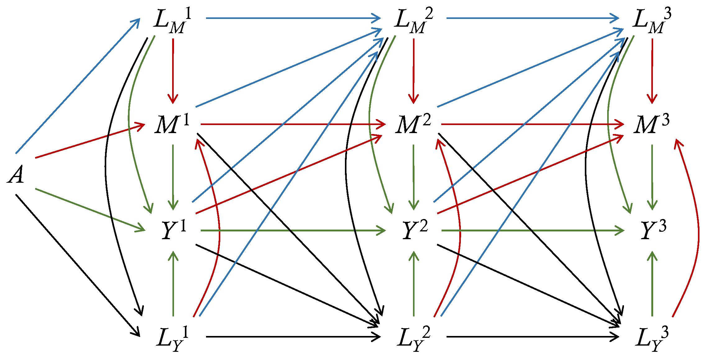
Ignorability simply means that the treatment is independent of all potential variables. The first independence in the sequential ignorability means that the treatment mechanism is ignorable given baseline covariates. At the period k, given all the observed variables prior to (or , ) including baseline covariates and observed treatment, the observed (or , ) are independent of all potential variables later than (or , ). Every post-treatment variable is as-if-randomized given the observed variables prior to the current time. To make the sequential ignorability assumption hold, unmeasured confounding between any two of , , and should be excluded (). Figure 1 displays a directed acyclic graph (DAG) that satisfies sequential ignorability. To derive the potential outcome , we set and at the level under the treatment , and set and at the level under the treatment , given the baseline covariates and history. No unmeasured confounding is allowed on the graph.
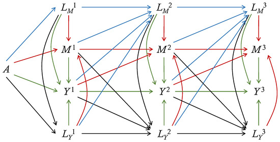
Figure 1.
A direct acyclic graph (DAG) for longitudinal outcomes with 3 periods. Here, A is the treatment, is the mediator-inducing confounding, is the outcome-inducing confounding, is the mediator and is the outcome at period j. The baseline covariates , which can have direct edges to all variables, are omitted. Red lines depict edges into the mediator, blue lines depict edges into the mediator-inducing confounding, green lines depict edges into the outcome, and black lines depict adges into the outcome-inducing confounding. This DAG also satisfies Markovness.
In the presence of censoring, let , , and be the censoring indicators for , , M and Y, respectively, at period k. The censoring indicator equals 1 if the variable is observed and 0 if the variable is missing. We assume that the censoring is random given the observed history, not depending on potential variables. The random censoring assumption we use here is weaker than the non-informative censoring assumption usually made in survival analysis literature which assumes the censoring is independent of all potential variables, as we allow the censoring probability being explained by the time-varying observed variables.
Assumption 4
(Random censoring for longitudinal outcomes). For ,
In addition, we assume the positivity. The supports of potential variables should overlap between hypothetical treatments and the censoring time should be large enough so that we have information about the variable distributions at every period.
Assumption 5
(Positivity for longitudinal outcomes). The following statements hold:
for every .
Under ignorability, sequential ignorability, consistency and random censoring, we can show that (see Appendix A)
We take the expectation for over the distribution of all potential variables using the g-formula [23]. Under positivity, the expectation of the potential outcome of interest at period K is identified as
The integration is conducted over the support of . We summarize the result in the following theorem.
Theorem 1.
Under Assumptions 1–5, NDE and NIE are identifiable.
The model involves more predictors with k growing larger. Estimation becomes more complicated if the measurements have too many periods. For simplicity, we may assume Markovness (exclusion restriction) that the potential variables at period k only rely on the preceding variables for at most one period.
Assumption 6
(Markovness for longitudinal outcomes). For ,
in which , , and are consistent with the history , , and .
Under Assumption 6,
So, we can use a pooled model to estimate these conditional probabilities. Then, the expectation of potential outcome can be estimated by the g-formula. An alternative to estimate the target estimand is to employ weighting methods [24].
2.2. Identifiability by Dismissible Treatment Components
The identification by sequential ignorability bears complexity in notations as well as difficulty in interpretations. An interventionist approach to studying mediation effects is the separable effects framework [11,13,21]. The initial treatment A is divided into two components and , where exerts effects on the mediator-inducing confounding and mediators , while exerts effects on the outcome-inducing confounding and outcomes . All post-treatment variables are potential outcomes of and . Since we are not to intervene in post-treatment variables, there is no need to express the post-treatment variables as potential outcomes of their history. In the realized experiment, , but in hypothetical or future experiments, we can let .
Specifically, we have the potential mediator-inducing confounding , the potential outcome-inducing confounding , the potential mediator and the potential outcome of interest at period k. Let be the baseline covariates. Denote the history for the mediator-inducing confounding, outcome-inducing confounding, mediator and outcome at period k by , , and , respectively, including all the post-treatment variables prior to this variable under the hypothetical treatment components . Let , , and be the observed mediator-inducing confounding, outcome-inducing confounding, mediator and outcome at period k. Let , , and be the observed history at period k. We assume that the observed variables are equal to the potential counterparts under the realized treatment.
Assumption 7
(Consistency). For ,
Under the separable effects framework, the natural direct effect (NDE) and natural indirect effect (NIE) on the outcome of interest at period K are defined as
In the literature on separable effects, these estimands are also called the separable direct effect (SDE) and separable indirect effect (SIE).
We assume the treatment mechanism is ignorability (the same role as the first part in Assumption 3).
Assumption 8
(Ignorability for longitudinal outcomes).
The core assumption for identification is the dismissible treatment components assumption, an alternative to sequential ignorability.
Assumption 9
(Dismissible treatment components for longitudinal outcomes).
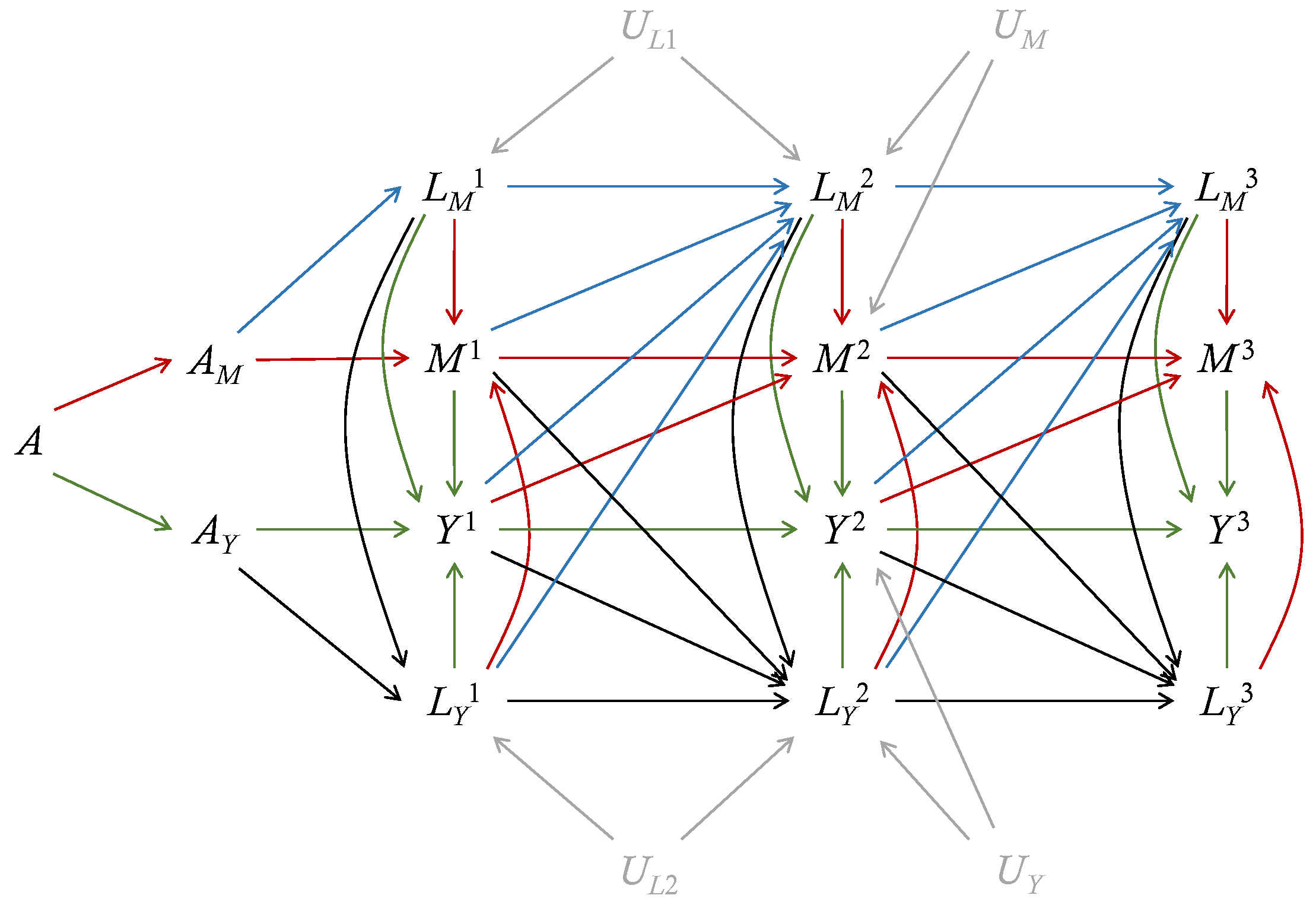
The dismissible treatment components assumption implies that the discrete-time hazards of the mediator-inducing confounding and mediators are irrelevant to , while the discrete-time hazards of the outcome-inducing confounding and outcomes are irrelevant to , given the baseline covariates and history. This assumption bypasses the complicated derivation of sequential ignorability by using more concise and interpretable notations. Figure 2 shows the extended DAG for longitudinal outcomes under the separable effects framework. Even if there is unmeasured confounding between and , or between and , the paths to deliver effects of on are blocked by the conditioning on the history (). Similarly, if there is unmeasured confounding between and , or between and , the paths to deliver effects of on are blocked by the conditioning on the history (). When such confounding exists, the sequential ignorability fails but the dismissible treatment components assumption holds. The dismissible treatment components assumption holds as long as there is no unmeasured confounding between the sequences of and , under which the effects of and can be isolated. Therefore, the dismissible treatment components assumption has weaker implications than the sequential ignorability.
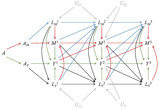
Figure 2.
An extended direct acyclic graph (eDAG) for longitudinal outcomes with 3 periods. The treatment A is divided into two components: and . In addition, is the mediator-inducing confounding, is the outcome-inducing confounding, is the mediator, and is the outcome at the period j. The baseline covariates , which can have direct edges to all variables, are omitted. Red lines depict edges into the mediator, blue lines depict edges into the mediator-inducing confounding, green lines depict edges into the outcome, black lines depict edges into the outcome-inducing confounding, and grey lines depict unmeasured confounding. In the presence of unmeasured confounding , , and , the dismissible treatment components assumption holds but the sequential ignorability assumption is violated.
Let , , and be the censoring indicator of , , M and Y, respectively, at period k. In addition to dismissible treatment components, we need random censoring and positivity.
Assumption 10
(Random censoring for longitudinal outcomes). For ,
Assumption 11
(Positivity for longitudinal outcomes). The following statements hold:
for every .
Assumptions 10 and 11 have similar meanings to Assumptions 4 and 5. Under ignorability, dismissible treatments components and random censoring, we can show that
by directly utilizing the property of the dismissible treatment components. Then, it is straightforward to apply the g-formula to identify the expectation of the potential outcome of interest under positivity:
The identification formula under the separable effects framework is identical to that under sequential ignorability. Although these two frameworks introduce different estimands with different interpretations, the assumptions incorporated have the same goal to eliminate cross-world quantities. The cross-world reliance is erased by conditioning on observed history. We summarize the identification results in the following theorem.
Theorem 2.
Under Assumptions 7–11, both NIE and NDE are identifiable.
A practically useful assumption is Markovness, which simplifies the conditional probabilities.
Assumption 12
(Markovness for longitudinal outcomes). For ,
Then, we only need to involve the most recent measurements of , , M and Y as well as and A in the conditional distribution model. A regression estimator and a weighting estimator for the natural effects under Markovness with competing events has been proposed [21]. This idea can be generalized to longitudinal mediation analysis by finding plug-in estimators using the identification formula. Theoretically, we can derive the efficient influence functions for each term in the identification formula of and then apply the functional delta method to obtain an efficient estimator for [19,25]. The resulting estimator may enjoy some multiple robustness based on the efficient influence functions. However, the efficient estimator can be very complicated, involving too many models. The multiple robustness may not be very meaningful since the regression models are often incorrectly specified simultaneously. The variance derived by the asymptotic form based on efficient influence functions can be unstable. In practice, simple estimators with sensitivity analysis are desired.
3. Time-to-Event Outcomes
Mediation analysis for time-to-event outcomes is referred to as semi-competing risks [26,27]. There is an intermediate event (counterpart to the mediator) and a terminal event (counterpart to the outcome). If the terminal event occurs at time t, then the intermediate event would never occur after t. Semi-competing risks can be understood by discretion of the continuous time. Let be a sequence of times, and the statuses of intermediate event and terminal event be measured at each time. The indicator of status equals 0 if the event has not occurred at time k and 1 if the event has already occurred at time k. Considering the nature of binary status, the conditional probabilities of and given the history can be expressed by the hazard using counting processes, that is, the timewise probability of occurring the event at k given the baseline and history prior to k.
Formally, we use the notion of counting processes to formalize the mediation analysis for time-to-event outcomes [22,27]. Suppose there are time-varying intermediate event-inducing confounding and terminal event-inducing confounding . Let
be the counting process of the potential intermediate event when the treatment is set at , the intermediate event process prior to t is set at , the terminal event process prior to t is set at , the intermediate event-inducing confounding process prior to t is set at and the terminal event-inducing confounding process prior to t is set at , . Analogously, let
be the counting process of the terminal event when the treatment is set at , and the processes prior to t are set at , , and , . Let be the baseline covariates, and the confounding processes of intermediate event-inducing confounding and terminal event-inducing confounding
respectively.
Let , , and be the counting processes of the intermediate event, terminal event, intermediate event-inducing confounding and terminal event-inducing confounding in the realized trial at time . We assume consistency if under the observed treatment A, the observable counting processes are compatible with the potential processes.
Assumption 13
(Consistency). For ,
The sequential ignorability assumption and dismissible treatment components assumption can be extended to time-to-event outcomes from discrete times. Sequential ignorability requires that there is no unmeasured confounding between any two processes at any two times [22]. This requirement is sometimes too strong, because the processes can be determined by some underlying features. It is hard to imagine timewise randomization for the processes. The dismissible treatment components assumption only requires that there is no unmeasured confounding between the processes of and , which is weaker than sequential ignorability. Therefore, we only formalize the assumptions under the separable effects framework.
When conducting mediation analysis, we would set the treatment for the intermediate event-inducing confounding and intermediate event at , and set the treatment for the terminal event-inducing confounding and terminal event at . Therefore, we have natural processes of the intermediate event-inducing confounding, terminal event-inducing confounding, intermediate event and terminal event , , and , respectively. The natural direct effect (NDE) and natural indirect effect (NIE) are defined by contrasting the counterfactual cumulative incidence of the terminal event:
Given the baseline covariates and natural processes, the continuous-time hazards of the intermediate event and terminal event can be expressed as
and the transition density of the intermediate event-inducing confounding to and terminal event-inducing confounding to at time t as
respectively. The treatment components and should have separable effects on and . In other words, given the baseline covariates and processes history, all the paths from to are blocked, and all the paths from to are blocked.
Assumption 14
(Ignorability for continuous time).
Assumption 15
(Dismissible treatment components for continuous time). For ,
If , we would not record the observations after t anymore. Since the counting processes can only jump from 0 to 1, the hazard of an event is only meaningful when the individual is at risk of this event. We can further simplify the notations,
To account for censoring, let be the censoring process. We assume that the processes of intermediate event-inducing confounding, terminal event-inducing confounding, intermediate event and terminal event at time t are either observed or censored simultaneously. We assume random censoring and positivity.
Assumption 16
(Random censoring for continuous time).
Assumption 17
(Positivity for continuous time).
Positivity ensures that the at-risk set has positive probability so we have data to estimate the hazards and transition densities.
Theorem 3.
Under Assumptions 13–17, NIE and NDE are identifiable for .
The identification formula is complicated but the idea is intuitive. Through product limits, the counterfactual cumulative incidence can be expressed as product limits of hazards (or conditional density) of counterfactual variables [28,29]. With the dismissible treatment assumption within the separable effects framework, the hazards (or conditional density) are identical to the observed counterparts by substituting the counterfactuals with the observables. For ,
where the inner integration is conducted over the support of and the outer integration is conducted over the support of . The first term is the incidence of the terminal event without a history of intermediate event, and the second term is the incidence of the terminal event with a history of intermediate event. Usually, the time-varying confounding can only change values at finite time points, so the transition density can be parameterized as a product of the density of the time to change values and the distribution function when changing values [28].
We can additionally assume Markovness to simplify the identification. The hazard and transition density only depend on the current status rather than the full history given baseline covariates.
Assumption 18
(Markovness for continuous time). For ,
Although Markovness is not necessary for identification, it brings great convenience for estimation. Under Markovness, we can use typical survival models like the proportional hazards model with time-varying confounding to estimate the hazards. If Markovness does not hold, the time origins of the transitions from the intermediate event to the terminal event are not aligned. There would be a biased sampling issue since the censoring probability is varying with time [30]. More deliberate models are required to obtain a closed-form estimator without Markovness. An estimator for the counterfactual cumulative incidence using parametric models based on efficient influence functions when there are no time-varying confounding has been proposed for semi-competing risks, i.e., illness–death models [31]. Multiple robustness found that the resulting estimator is consistent if (1) all three transition hazards are correctly specified or (2) the propensity score and censoring probability are correctly specified, and two of the three transition hazards are correctly specified. Theoretically, this idea can be generalized to the case with time-varying confounding under semiparametric models using the functional delta method, but there is no easy-to-implement estimating procedure if there are too many time-varying covariates or the time-varying covariates are too complex.
4. Application to Stem Cell Transplantation Data
Allogeneic stem cell transplantation is a widely applied therapy to treat acute lymphoblastic leukemia (ALL), including two sorts of transplant modalities: human leukocyte antigen (HLA)-matched sibling donor transplantation (MSDT) and haploidentical stem cell transplantation from family (Haplo-SCT). MSDT has long been regarded as the first choice of transplantation because MSDT leads to lower transplant-related mortality (TRM), also known as non-relapse mortality (NRM) [32]. Another source of mortality is due to relapse, known as relapse-related mortality (RRM). In recent years, some benefits of Haplo-SCT have been noticed in that patients with positive pre-transplantation minimum residual disease (MRD) undergoing Haplo-SCT have better prognosis in relapse, and hence lower relapse-related mortality [33]. It is of interest to study how the transplant modalities exert effects on overall mortality.
A total of patients with positive MRD undergoing allogeneic stem cell transplantation were included in our study [22,34]. Among these patients, 65 received MSDT () and 238 received Haplo-SCT (). The transplantation type is “genetically randomized” in that there is no specific consideration to prefer Haplo-SCT over MSDT whenever MSDT is accessible [33]. Therefore, we expect ignorability. Four baseline covariates were considered: age, sex (male, female), diagnosis (T-ALL or B-ALL) and complete remission status (CR1, CR>1). A time-varying covariate is the occurrence of graft-versus-host disease (GVHD). These five covariates are risk factors associated with relapse and mortality indicated in the previous literature. The outcome is of the time-to-event type, subject to right censoring. The mean follow-up time was 1336 days. The terminal event is overall mortality, and the intermediate event is relapse. In the MSDT group, 47.7% patients were observed to encounter relapse and 53.8% mortality. In the Haplo-SCT group, 30.0% patients were observed to encounter relapse and 36.6% mortality. Summary statistics are presented in Table 1.

Table 1.
Summary statistics in the data application, stratified by treatment groups. We list the mean and standard deviation (SD) of baseline covariates in each group. We also list the proportion of certain observed uncensored events (GVHD, relapse, mortality) and the time to the observed uncensored event in each group.
We adopt the separable effects framework to study the mediation effect of transplant modalities on overall mortality. We can find clinical interpretation for the treatment components. Haplo-SCT has fewer matched HLA loci compared with MSDT, so stronger immune rejection is anticipated. In practice, patients receiving Haplo-SCT should additionally use antithymocyte globulin (ATG) to facilitate engraftment [35]. Therefore, is the treatment component that, through delaying immune reconstitution (the combined use of ATG), increases the risk of transplant-related mortality. Relapse is caused by the presence of minimum residual disease. The stronger immune rejection with Haplo-SCT kills body cells but also kills the minimum residual disease cells, which are referred to as the graft-versus-host and graft-versus-leukemia (GVL) effects, respectively [33]. Therefore, is a treatment component through GVHD, which increases the risk of GVHD but reduces the risk of relapse. Let be the time-varying GVHD status, affected by . Following the notations in the preceding section, is null.
In the presence of time-varying covariates, it is very difficult to apply the g-formula to obtain a simple regression estimator, because there are too many terms in the identification formula. Taking advantage of the fact that the occurrence of GVHD is binary, we may as well consider the GVHD as a state within the multi-state model. In this way, there are a total of four states, the initial state, the GVHD state, the relapse state and the mortality state, as shown in Figure 3. The x-axis is the day after transplantation, and the y-axis is on the scale of cumulative incidence. To avoid bidirectional transition between GVHD and relapse, we can further divide the GVHD state into an acute GVHD state (after treatment but before relapse) and a chronic GVHD state (after relapse but before mortality). By modeling the transition hazards between states, we can derive the cumulative incidence function of the overall mortality through integrating functions of hazards.
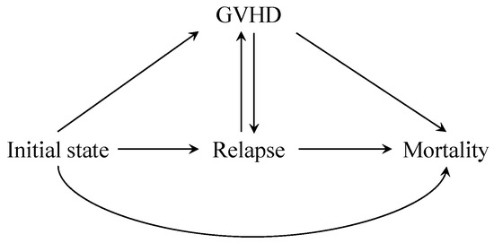
Figure 3.
A multi-state model illustration for the leukemia data. Relapse is the intermediate event (), mortality is the terminal event () and GVHD status is a time-varying covariate taking values 0 or 1 (). To ease estimation, we regard GVHD as a state. GVHD can transit to relapse and relapse can transit to GVHD. Within the separable effects framework, the treatment component has an effect on the hazard of mortality (), whereas the treatment component has effects on the hazard of GVHD () and relapse ().
We impose a semiparametric proportional hazards model for the transition rates with Markovness:
where , and are unknown baseline hazards. The baseline hazards can be different across treatment groups. Specially, the hazards of mortality and GVHD can rely on the status of relapse. The statuses of the intermediate event and confounding serve as time-varying covariates in the extended Cox model [36,37]. The censoring probability is also estimated by the semiparametric proportional hazards model. The unknown parameters in the above models are estimated by nonparametric maximum likelihood estimation (NPMLE), where the estimated baseline hazards are step functions with jumps only at observed event times [38]. The estimated parameters are updated by the Newton–Raphson algorithm and are considered to be converged if the update leads to changes in values smaller than 0.0001. The estimation procedure is implemented using R (version 4.4.0) [39].
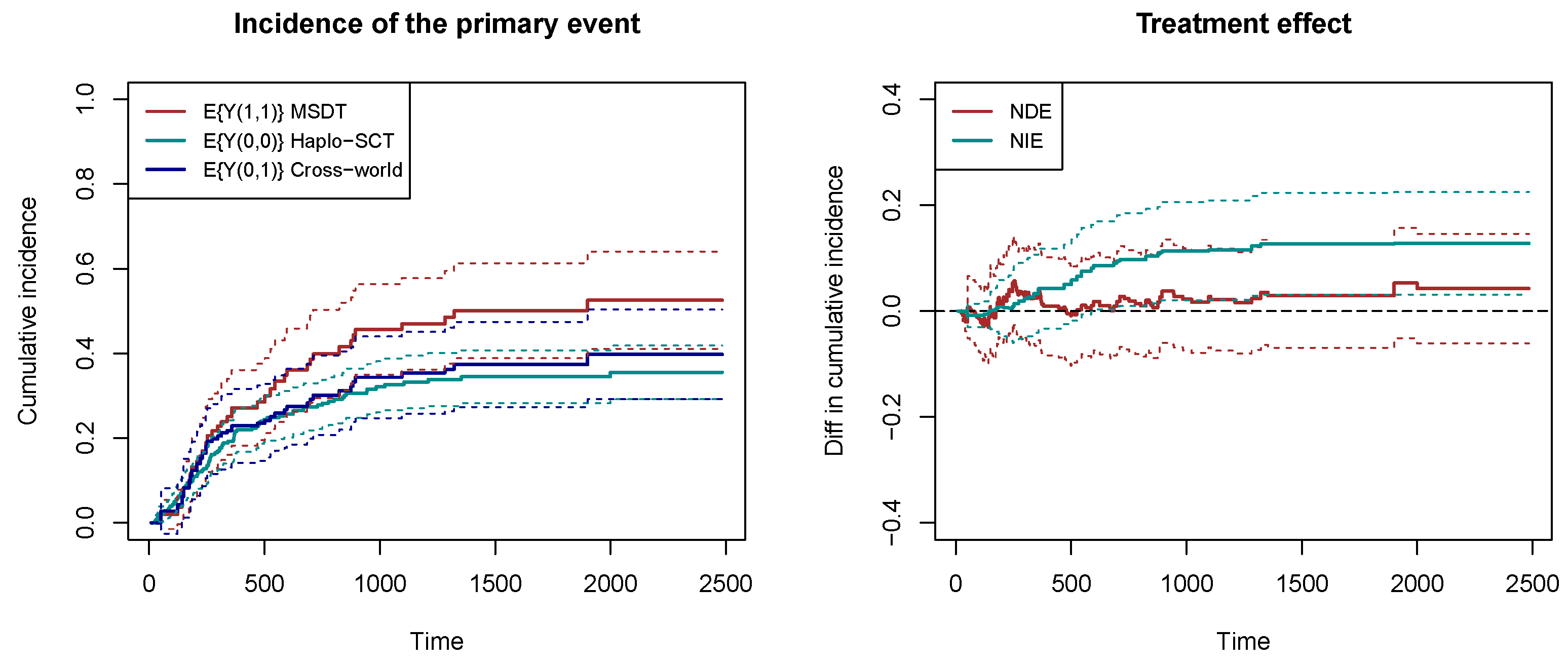
Figure 4 shows the estimated counterfactual cumulative incidences of overall mortality in the left panel. The 95% confidence intervals are obtained by bootstrap with 200 resamplings. The red line represents the cumulative incidence of mortality when receiving MSDT, and the cyan line represents the cumulative incidence of mortality when receiving Haplo-SCT. We can see that the mortality rate is higher for MSDT in MRD-positive patients, indicating a stronger graft-versus-leukemia effect for Haplo-SCT. In a hypothetical world, suppose that the delayed immune reconstitution is set at the level for Haplo-SCT , and the GVHD/GVL is set at the level for MSDT . Then, the blue line represents the cumulative incidence of mortality in this hypothetical world. The right panel of Figure 4 shows the natural direct effect (NDE) and natural indirect effect (NIE). The natural indirect effect is significantly positive, indicating that Haplo-SCT reduces the risk of overall mortality through reducing the risk of relapse. The natural direct effect is insignificant, which means that the usage of ATG to delay immune reconstitution does not have a high impact on mortality.
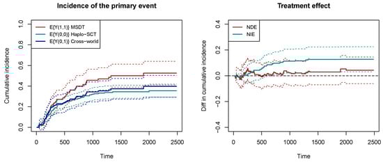
Figure 4.
The counterfactual cumulative incidence functions and the natural direct/indirect effects. The dashed lines represent the 95% bootstrap confidence intervals.
A sensitivity analysis can be conducted by assuming that chronic GVHD is a terminal event-inducing confounding, or assuming that both acute GVHD and chronic GVHD are terminal event-inducing confoundings. Fortunately, the estimated cumulative incidences and treatment effects are similar to those in Figure 4. This strengthens our conclusion. The empirical findings provide guidance on allogeneic stem cell transplantation. Since Haplo-SCT is more accessible than MSDT, we argue the Haplo-SCT is a reasonable alternative to MSDT. Although Haplo-SCT may lead to slightly higher non-relapse mortality, it is promising that practitioners pay special attention to patients receiving Haplo-SCT in order to reduce relapse-related mortality. The overall mortality can be significantly reduced due to the strong graft-versus-leukemia effect of Haplo-SCT.
5. Conclusions
The estimand in mediation analysis involves cross-world quantities. In this article, we studied two assumptions for mediation analysis, namely, sequential ignorability and dismissible treatment components. The former is conventional in mediation analysis and can be understood from the view of sequential randomization. The latter comes from the separable effects framework. The dismissible treatment components condition is weaker than sequential ignorability because the former allows some types of unmeasured confounding. The dismissible treatment components can be tested in future experiments if the treatment components are known. It is easier to interpret the dismissible treatment components assumption than sequential ignorability. Even if the dismissible treatment components assumption is violated, the estimands of natural direct and indirect effects are still meaningful, although not identifiable. Nowadays, in medical studies, the separable effects framework is becoming more and more popular. For time-to-event outcomes, the advantage of the separable effects framework is significant due to its notational simplicity and interpretability.
Through the application of real data on allogeneic stem cell transplantation, we show the usefulness of the separable effects framework. A post-treatment time-varying covariate, GVHD, is considered to modify the treatment effect. We find that Haplo-SCT reduces the risk of overall mortality through reducing the risk of relapse. Haplo-SCT has the potential to serve as an alternative to MSDT. In this real-data example, we have explicit interpretation for the separable effects. Conclusions drawn from the separable effects framework can inform new clinical knowledge, and also inspire biological research on the micro-foundation of treatment components.
6. Discussion
The separable effects framework has some limitations. The dismissible treatment components assumption is not testable in real-world trials. In the presence of time-varying confounding, it is essential to discuss with subject experts to determine whether the time-varying confounding is intermediate event-inducing or terminal event-inducing. If the classification of time-varying confounding is ambiguous, sensitivity analysis is encouraged. The sequential ignorability framework can be more useful in this case. We can find a certain type of natural direct effect or path-specific effect that is identifiable, and this partial effect may be of scientific interest [15,16].
Although the identifiability of the natural direct and indirect effects is proven, estimation remains challenging. The regression estimator using g-formula is not only complicated but also subject to model mis-specification. It is still worth studying how to derive more efficient estimators relying on weaker model assumptions. Since the estimation of cumulative incidence is recursive, slight model mis-specification may lead to a huge estimation bias at large time points. Modeling multiple and multi-valued time-varying covariates can be extremely difficult, so existing studies only focused on simple time-varying covariates [28]. In the application, the time-varying covariate is binary, so we take advantage of multi-state models to derive the cumulative incidence. It is questionable whether desirable statistical properties can be maintained in the presence of complex time-varying covariates.
There are a few future research directions. First, the asymptotic property of the estimators is complicated in longitudinal studies by applying the g-formula. Theoretically, the asymptotic property can be established based on the influence function. However, the influence function is too tedious to derive and there is no efficient algorithms to implement the g-formula in longitudinal studies with too many periods. Second, mediation analysis requires that the treatment lasts from the beginning to end without noncompliance. In longitudinal studies and time-to-event studies, patients may switch to other treatments at some time [19,40]. A new problem is how to define the estimand and formalize identification assumptions. Third, in the separable effects framework, it is possible to decompose the initial treatment into more components. Maybe there is a separable treatment component that influences time-varying covariates. Third, the direct outcome event following the treatment and the indirect outcome event following the intermediate event may be contributed by different treatment components. Therefore, the total effect should be decomposed into more than two natural effects [29]. Furthermore, there can be multiple mediators or intermediate events. It is worth studying the decomposition, identification and estimation with more complex treatment–mediator–outcome structures [41,42,43].
Another type of mediation estimand is the randomized interventional effects [40,44,45]. In general cases, the randomized interventional effects are distinct from the natural effects (or separable effects). The randomized interventional effects randomly draw post-treatment mediators and confoundings from the observed distribution associated with a given treatment policy. Weaker assumptions are required to identify the treatment effects. The identification assumptions can be understood from the view of nonparametric structural equation models for the data generating process of the time-varying treatments, confoundings, mediators and outcomes. It is not necessary to separate the post-treatment confounding into several components associated with treatment components for identification. Sequential doubly robust estimation can be used to estimate the treatment effects [46,47]. The idea of randomized interventional effects has the potential to be generalized to time-to-event outcomes [48].
Author Contributions
Conceptualization, Y.D.; methodology, Y.D. and H.W.; investigation, Y.D., H.W. and X.X.; writing—original draft, Y.D.; writing—review and editing, Y.Z. and Y.H. All authors have read and agreed to the published version of the manuscript.
Funding
This work is supported by the Science and Technology Project of Guangxi (Guike AD21220114); the National Key Research and Development Program of China, Grant No. 2021YFF0901400; and the National Natural Science Foundation of China, Grant No. 12026606, 12226005, 12361055.
Data Availability Statement
The data and R (version 4.4.0) codes that support our findings are available on GitHub https://github.com/naiiife/multistate (accessed on 22 July 2024).
Acknowledgments
We thank the Guest Editor for the invitation. We thank Yuewen Wang at Peking University People’s Hospital for introducing the background of allogeneic stem cell transplantation.
Conflicts of Interest
Author Xia Xiao was employed by the Geely Automobile Holdings Limited. The remaining authors declare that the research was conducted in the absence of any commercial or financial relationships that could be construed as a potential conflict of interest. The Geely Automobile Holdings Limited had no role in the design of the study; in the collection, analyses, or interpretation of data; in the writing of the manuscript, or in the decision to publish the results.
Appendix A. Proof of Theorem 1
We only prove for . In the following proof, we use the caption A1 (Assumption 1), A2 (Assumption 2), … in each line to illustrate which assumption is used to derive the equation. Other proofs are similar.
Positivity (A5) ensures that the conditional probability is well defined. Finally, by the g-formula, we obtain the identification expression for :
References
- Baron, R.M.; Kenny, D.A. The moderator–mediator variable distinction in social psychological research: Conceptual, strategic, and statistical considerations. J. Personal. Soc. Psychol. 1986, 51, 1173–1182. [Google Scholar] [CrossRef] [PubMed]
- Robins, J.M.; Greenland, S. Identifiability and exchangeability for direct and indirect effects. Epidemiology 1992, 3, 143–155. [Google Scholar] [CrossRef] [PubMed]
- Tchetgen, E.J.T.; Shpitser, I. Semiparametric theory for causal mediation analysis: Efficiency bounds, multiple robustness, and sensitivity analysis. Ann. Stat. 2012, 40, 1816–1845. [Google Scholar] [CrossRef] [PubMed]
- Pearl, J. Interpretation and identification of causal mediation. Psychol. Methods 2014, 19, 459–481. [Google Scholar] [CrossRef] [PubMed]
- Imai, K.; Keele, L.; Tingley, D. A general approach to causal mediation analysis. Psychol. Methods 2010, 15, 309. [Google Scholar] [CrossRef] [PubMed]
- Imai, K.; Keele, L.; Yamamoto, T. Identification, inference and sensitivity analysis for causal mediation effects. Stat. Sci. 2010, 25, 51–71. [Google Scholar] [CrossRef]
- Fiedler, K.; Schott, M.; Meiser, T. What mediation analysis can (not) do. J. Exp. Soc. Psychol. 2011, 47, 1231–1236. [Google Scholar] [CrossRef]
- Lok, J.J. Defining and estimating causal direct and indirect effects when setting the mediator to specific values is not feasible. Stat. Med. 2016, 35, 4008–4020. [Google Scholar] [CrossRef] [PubMed]
- Moreno-Betancur, M.; Carlin, J.B. Understanding interventional effects: A more natural approach to mediation analysis? Epidemiology 2018, 29, 614–617. [Google Scholar] [CrossRef] [PubMed]
- Lok, J.J.; Bosch, R.J. Causal organic indirect and direct effects: Closer to the original approach to mediation analysis, with a product method for binary mediators. Epidemiology 2021, 32, 412–420. [Google Scholar] [CrossRef] [PubMed]
- Robins, J.M.; Richardson, T.S. Alternative graphical causal models and the identification of direct effects. In Causality and Psychopathology: Finding the Determinants of Disorders and Their Cures; Oxford University Press: Oxford, UK, 2010; Volume 84, pp. 103–158. [Google Scholar]
- Robins, J.M.; Richardson, T.S.; Shpitser, I. An interventionist approach to mediation analysis. In Probabilistic and Causal Inference: The Works of Judea Pearl; ACM: New York, NY, USA, 2022; pp. 713–764. [Google Scholar]
- Stensrud, M.J.; Young, J.G.; Didelez, V.; Robins, J.M.; Hernán, M.A. Separable effects for causal inference in the presence of competing events. J. Am. Stat. Assoc. 2022, 117, 175–183. [Google Scholar] [CrossRef]
- Wodtke, G.T.; Zhou, X. Effect decomposition in the presence of treatment-induced confounding: A regression-with-residuals approach. Epidemiology 2020, 31, 369–375. [Google Scholar] [CrossRef] [PubMed]
- Miles, C.H.; Shpitser, I.; Kanki, P.; Meloni, S.; Tchetgen Tchetgen, E.J. On semiparametric estimation of a path-specific effect in the presence of mediator-outcome confounding. Biometrika 2020, 107, 159–172. [Google Scholar] [CrossRef] [PubMed]
- Xia, F.; Chan, K.C.G. Identification, semiparametric efficiency, and quadruply robust estimation in mediation analysis with treatment-induced confounding. J. Am. Stat. Assoc. 2023, 118, 1272–1281. [Google Scholar] [CrossRef]
- Bind, M.A.; Vanderweele, T.; Coull, B.; Schwartz, J. Causal mediation analysis for longitudinal data with exogenous exposure. Biostatistics 2016, 17, 122–134. [Google Scholar] [CrossRef] [PubMed]
- Jose, P.E. The merits of using longitudinal mediation. Educ. Psychol. 2016, 51, 331–341. [Google Scholar] [CrossRef]
- Zheng, W.; van der Laan, M. Longitudinal mediation analysis with time-varying mediators and exposures, with application to survival outcomes. J. Causal Inference 2017, 5, 20160006. [Google Scholar] [CrossRef] [PubMed]
- Ten Have, T.R.; Joffe, M.M. A review of causal estimation of effects in mediation analyses. Stat. Methods Med Res. 2012, 21, 77–107. [Google Scholar] [CrossRef] [PubMed]
- Stensrud, M.J.; Hernán, M.A.; Tchetgen Tchetgen, E.J.; Robins, J.M.; Didelez, V.; Young, J.G. A generalized theory of separable effects in competing event settings. Lifetime Data Anal. 2021, 27, 588–631. [Google Scholar] [CrossRef] [PubMed]
- Deng, Y.; Wang, Y.; Zhou, X.H. Direct and indirect treatment effects in the presence of semicompeting risks. Biometrics 2024, 80, ujae032. [Google Scholar] [CrossRef] [PubMed]
- Robins, J. A new approach to causal inference in mortality studies with a sustained exposure period—Application to control of the healthy worker survivor effect. Math. Model. 1986, 7, 1393–1512. [Google Scholar] [CrossRef]
- Young, J.G.; Stensrud, M.J.; Tchetgen Tchetgen, E.J.; Hernán, M.A. A causal framework for classical statistical estimands in failure-time settings with competing events. Stat. Med. 2020, 39, 1199–1236. [Google Scholar] [CrossRef] [PubMed]
- Wang, Z.; van der Laan, L.; Petersen, M.; Gerds, T.; Kvist, K.; van der Laan, M. Targeted maximum likelihood based estimation for longitudinal mediation analysis. arXiv 2023, arXiv:2304.04904. [Google Scholar]
- Fine, J.P.; Jiang, H.; Chappell, R. On semi-competing risks data. Biometrika 2001, 88, 907–919. [Google Scholar] [CrossRef]
- Huang, Y.T. Causal mediation of semicompeting risks. Biometrics 2021, 77, 1143–1154. [Google Scholar] [CrossRef]
- Rytgaard, H.C.; Gerds, T.A.; van der Laan, M.J. Continuous-time targeted minimum loss-based estimation of intervention-specific mean outcomes. Ann. Stat. 2022, 50, 2469–2491. [Google Scholar] [CrossRef]
- Deng, Y.; Wang, Y.; Zhan, X.; Zhou, X.H. Separable pathway effects of semi-competing risks via multi-state models. arXiv 2023, arXiv:2306.15947. [Google Scholar]
- Asgharian, M.; M’Lan, C.E.; Wolfson, D.B. Length-biased sampling with right censoring: An unconditional approach. J. Am. Stat. Assoc. 2002, 97, 201–209. [Google Scholar] [CrossRef]
- Breum, M.S.; Munch, A.; Gerds, T.A.; Martinussen, T. Estimation of separable direct and indirect effects in a continuous-time illness-death model. Lifetime Data Anal. 2024, 30, 143–180. [Google Scholar] [CrossRef] [PubMed]
- Kanakry, C.G.; Fuchs, E.J.; Luznik, L. Modern approaches to HLA-haploidentical blood or marrow transplantation. Nat. Rev. Clin. Oncol. 2016, 13, 10–24. [Google Scholar] [CrossRef] [PubMed]
- Chang, Y.J.; Wang, Y.; Xu, L.P.; Zhang, X.H.; Chen, H.; Chen, Y.H.; Wang, F.R.; Sun, Y.Q.; Yan, C.H.; Tang, F.F.; et al. Haploidentical donor is preferred over matched sibling donor for pre-transplantation MRD positive ALL: A phase 3 genetically randomized study. J. Hematol. Oncol. 2020, 13, 27. [Google Scholar] [CrossRef] [PubMed]
- Ma, R.; Xu, L.P.; Zhang, X.H.; Wang, Y.; Chen, H.; Chen, Y.H.; Wang, F.R.; Han, W.; Sun, Y.Q.; Yan, C.H.; et al. An Integrative Scoring System Mainly Based on Quantitative Dynamics of Minimal/Measurable Residual Disease for Relapse Prediction in Patients with Acute Lymphoblastic Leukemia. 2021. Available online: https://library.ehaweb.org/eha/2021/eha2021-virtual-congress/324642 (accessed on 12 June 2021).
- Walker, I.; Panzarella, T.; Couban, S.; Couture, F.; Devins, G.; Elemary, M.; Gallagher, G.; Kerr, H.; Kuruvilla, J.; Lee, S.J.; et al. Pretreatment with anti-thymocyte globulin versus no anti-thymocyte globulin in patients with haematological malignancies undergoing haemopoietic cell transplantation from unrelated donors: A randomised, controlled, open-label, phase 3, multicentre trial. Lancet Oncol. 2016, 17, 164–173. [Google Scholar] [CrossRef]
- Crowley, J.; Hu, M. Covariance analysis of heart transplant survival data. J. Am. Stat. Assoc. 1977, 72, 27–36. [Google Scholar] [CrossRef]
- Thackham, M.; Ma, J. On maximum likelihood estimation of the semi-parametric Cox model with time-varying covariates. J. Appl. Stat. 2020, 47, 1511–1528. [Google Scholar] [CrossRef] [PubMed]
- Zeng, D.; Lin, D. Maximum likelihood estimation in semiparametric regression models with censored data. J. R. Stat. Soc. Ser. B Stat. Methodol. 2007, 69, 507–564. [Google Scholar] [CrossRef]
- R Core Team. R: A Language and Environment for Statistical Computing; Version 4.4.0 [Computer Software]; R Foundation for Statistical Computing: Vienna, Austria, 2024. [Google Scholar]
- VanderWeele, T.J.; Tchetgen Tchetgen, E.J. Mediation analysis with time varying exposures and mediators. J. R. Stat. Soc. Ser. B Stat. Methodol. 2017, 79, 917–938. [Google Scholar] [CrossRef] [PubMed]
- Xia, F.; Chan, K.C.G. Decomposition, identification and multiply robust estimation of natural mediation effects with multiple mediators. Biometrika 2022, 109, 1085–1100. [Google Scholar] [CrossRef]
- Zhou, X. Semiparametric estimation for causal mediation analysis with multiple causally ordered mediators. J. R. Stat. Soc. Ser. B Stat. Methodol. 2022, 84, 794–821. [Google Scholar] [CrossRef]
- Wei, H.; Cai, H.; Shi, C.; Song, R. On efficient inference of causal effects with multiple mediators. arXiv 2024, arXiv:2401.05517. [Google Scholar]
- VanderWeele, T.J.; Vansteelandt, S.; Robins, J.M. Effect decomposition in the presence of an exposure-induced mediator-outcome confounder. Epidemiology 2014, 25, 300–306. [Google Scholar] [CrossRef] [PubMed]
- Rudolph, K.E.; Williams, N.T.; Diaz, I. Practical causal mediation analysis: Extending nonparametric estimators to accommodate multiple mediators and multiple intermediate confounders. Biostatistics 2024, kxae012. [Google Scholar] [CrossRef] [PubMed]
- Díaz, I.; Williams, N.; Rudolph, K.E. Efficient and flexible mediation analysis with time-varying mediators, treatments, and confounders. J. Causal Inference 2023, 11, 20220077. [Google Scholar] [CrossRef]
- Gilbert, B.; Hoffman, K.L.; Williams, N.; Rudolph, K.E.; Schenck, E.J.; Díaz, I. Identification and estimation of mediational effects of longitudinal modified treatment policies. arXiv 2024, arXiv:2403.09928. [Google Scholar]
- Díaz, I.; Hoffman, K.L.; Hejazi, N.S. Causal survival analysis under competing risks using longitudinal modified treatment policies. Lifetime Data Anal. 2024, 30, 213–236. [Google Scholar] [CrossRef] [PubMed]

Disclaimer/Publisher’s Note: The statements, opinions and data contained in all publications are solely those of the individual author(s) and contributor(s) and not of MDPI and/or the editor(s). MDPI and/or the editor(s) disclaim responsibility for any injury to people or property resulting from any ideas, methods, instructions or products referred to in the content. |
© 2024 by the authors. Licensee MDPI, Basel, Switzerland. This article is an open access article distributed under the terms and conditions of the Creative Commons Attribution (CC BY) license (https://creativecommons.org/licenses/by/4.0/).