

Modeling and Control of the High-Voltage Terminal of a Tandem Van de Graaff Accelerator
 ,
, 
Abstract
:1. Introduction
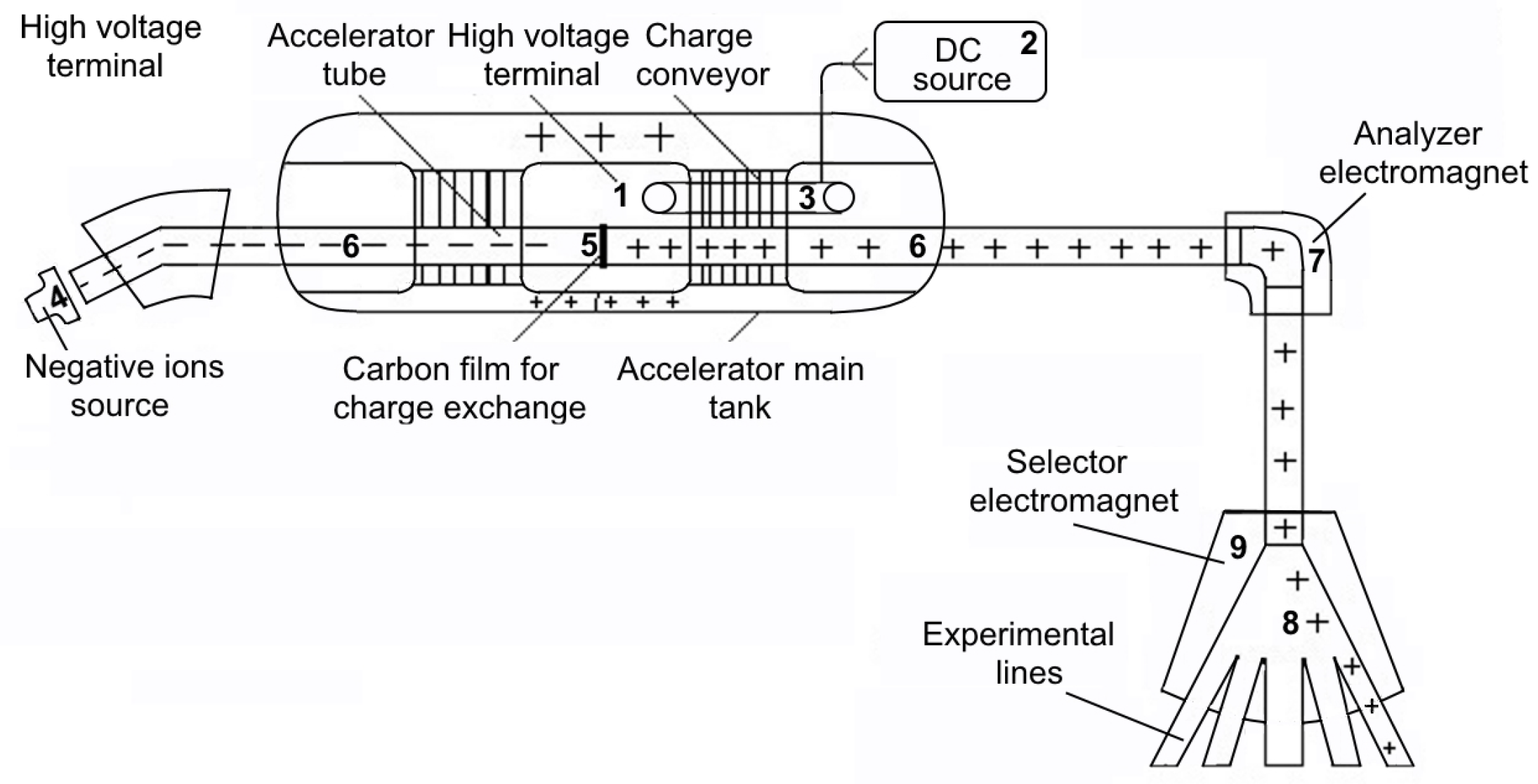
2. Tandem Van de Graaff Accelerator: General Overview
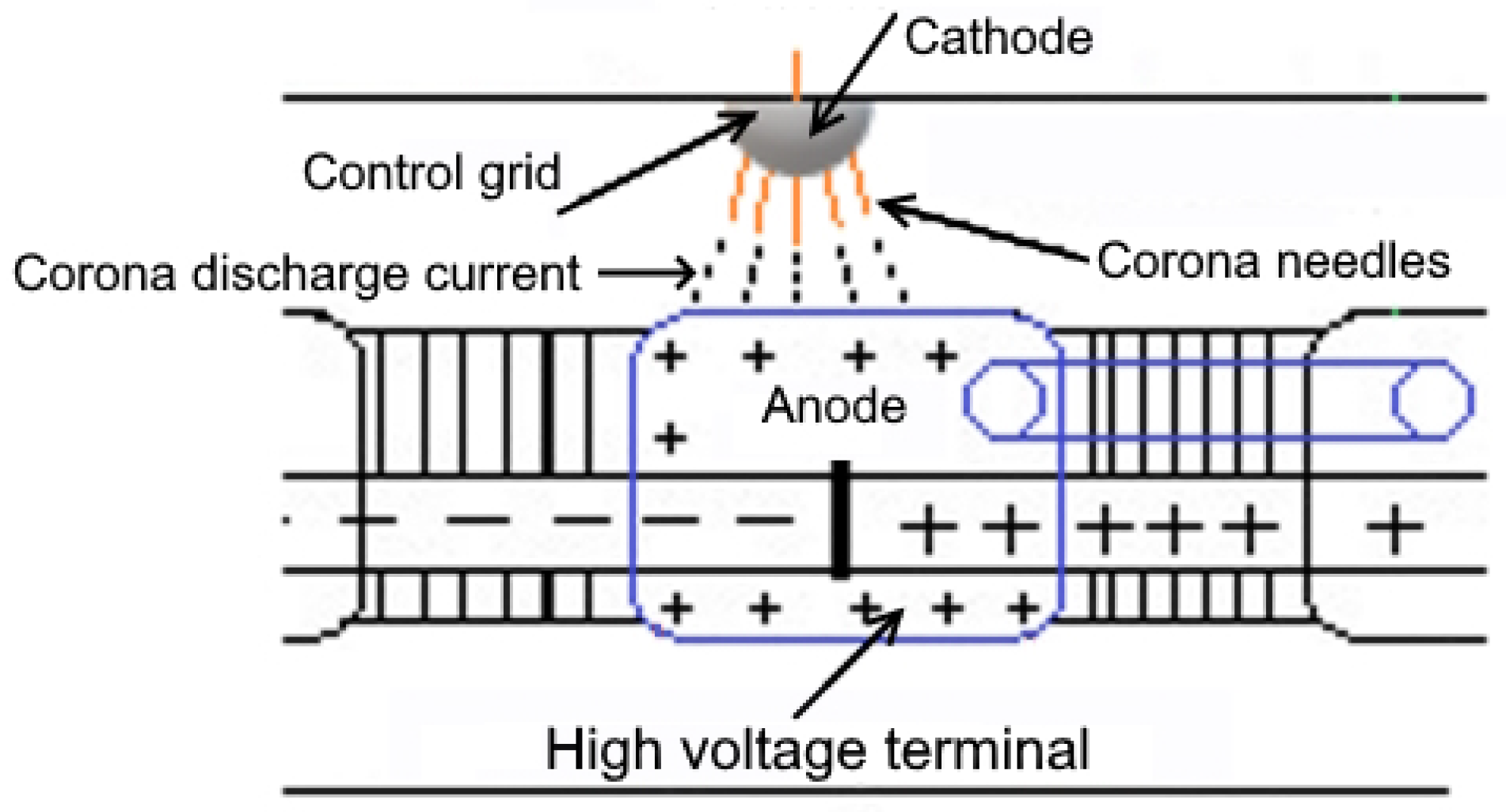
- Corona needles drain current from the terminal potential and, thus, vary its voltage.
- The generating voltmeter measures the terminal voltage in direct current (DC).
- The Pick-Off Capacitor (POC) measures voltage variations in Alternating Current (AC).
- SLITs monitor the position of the beam downstream of the analyzer electromagnet.
- The high-voltage terminal produces a high voltage that allows the acceleration of the particles (in the remainder of the document, the term “terminal” refers to the high-voltage terminal).
- The direct current source performs the transfer of the charge to the the terminal.
- The analyzer electromagnet behaves as a filter, which selects particles of a given energy.
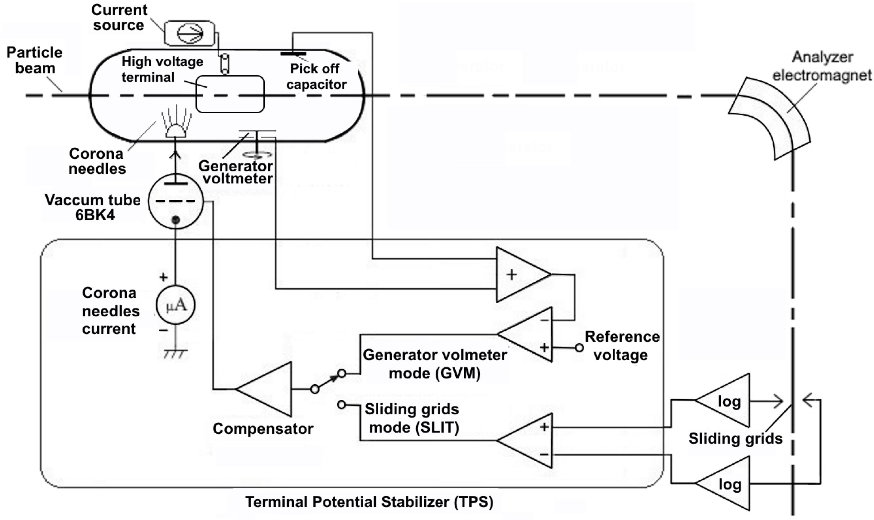
- Generating voltmeter mode (GVM): This mode is used when it is desired to set the terminal voltage to a specific value given by a reference signal associated with the energy of the particles to be accelerated. In this mode, a fast feedback signal from the POC is used to reduce the short-term ripple in combination with a slow feedback signal from the voltage measured by the generating voltmeter. A compensator provides a signal to control the current drained through the corona needles using a 6BK4 vacuum tube control grid (Radio Corporation of America (RCA), Harrison, NJ, USA.). The current drained through the corona needles provides the voltage control at the accelerator terminal.
- SLIT mode: This mode is put into operation when the particle beam is present after the analyzer electromagnet, which generates a current whose value is proportional to the beam position upon colliding with the SLITs. Once this position is monitored, it can be controlled by increasing or decreasing the terminal voltage by draining current from the terminal through the corona needles.
- Automatic mode: This mode allows an automatic switching between the GVM and the SLIT mode, depending mainly on the current in the SLITs. If the value of a current is greater than a previously set value on the SLITs, the system remains in SLIT mode. Otherwise, if the value of the current is less than that of the SLITs, the system switches to GVM mode, where the user can manually vary the terminal voltage until the beam current required to switch to SLIT mode is obtained.
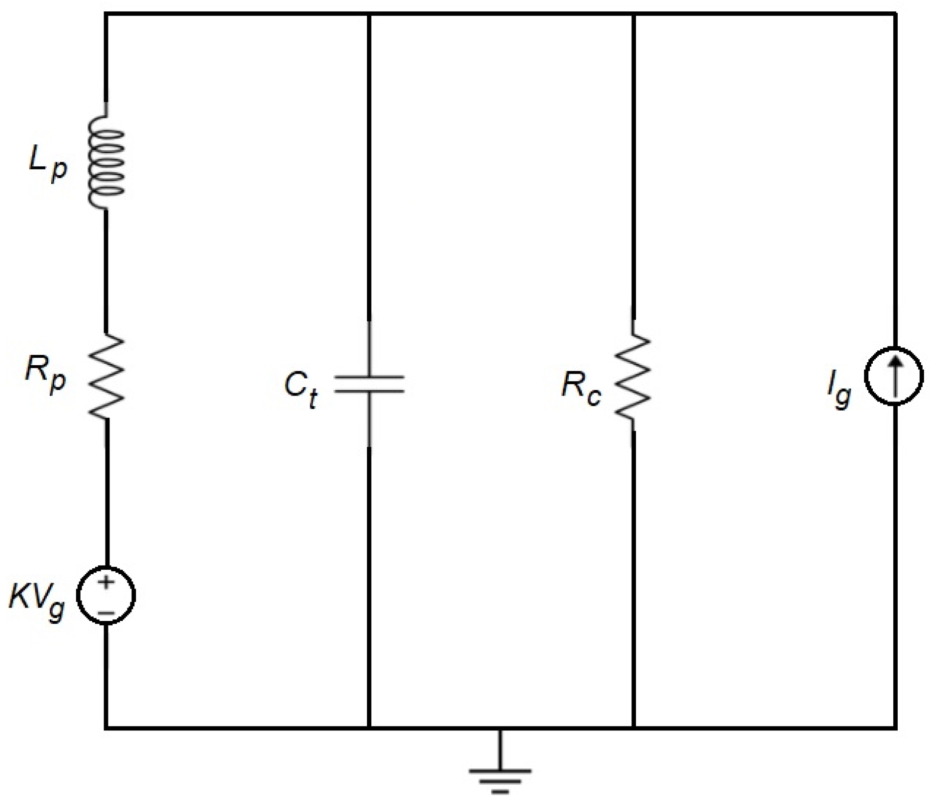
3. Mathematical Modeling
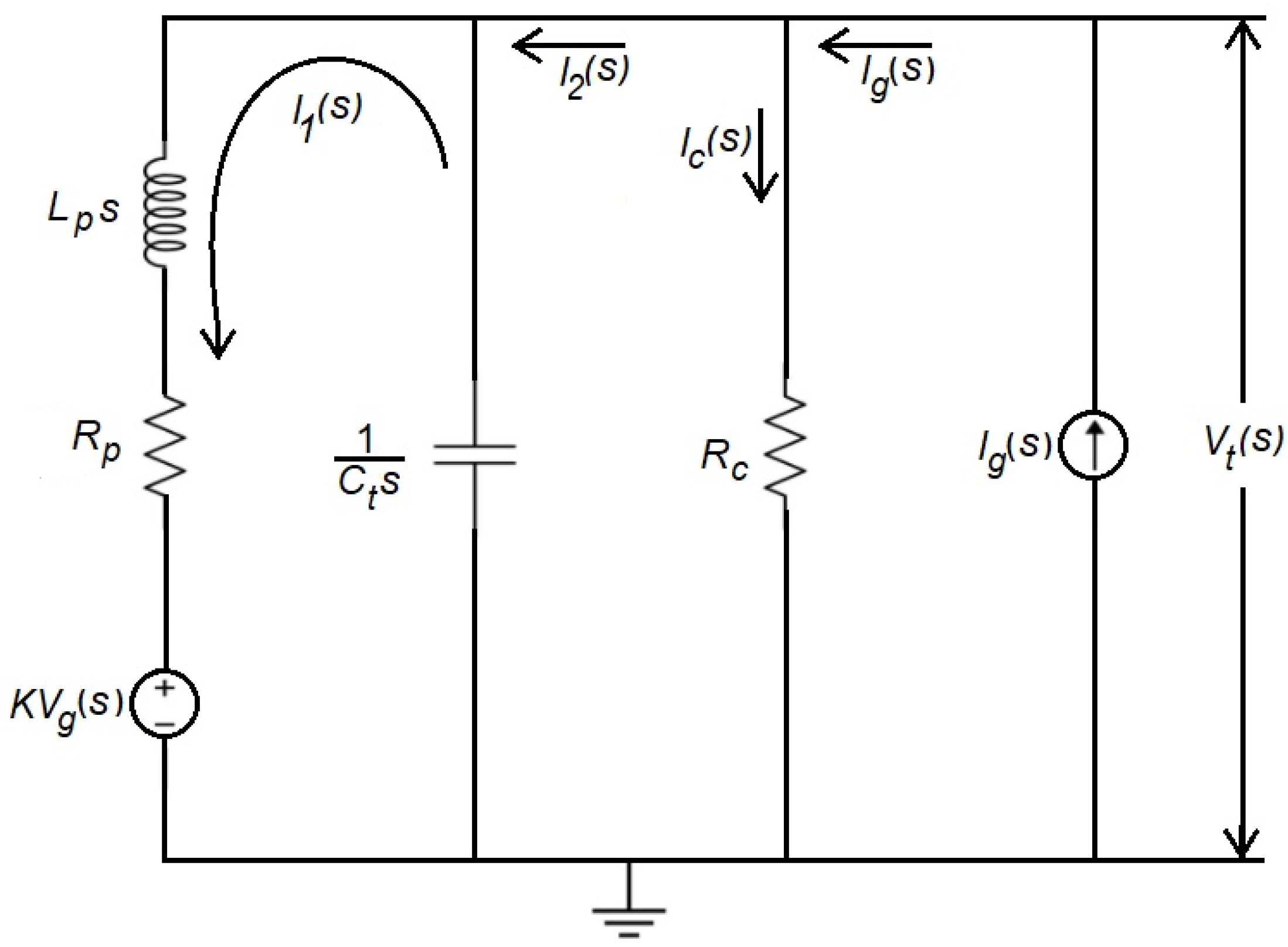
3.1. Model Considering an Equivalent Self-Inductance of the Corona Triode
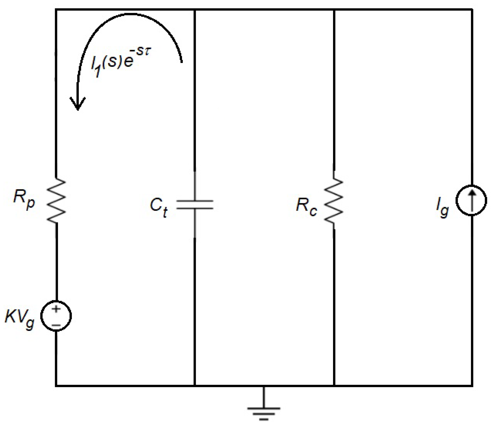
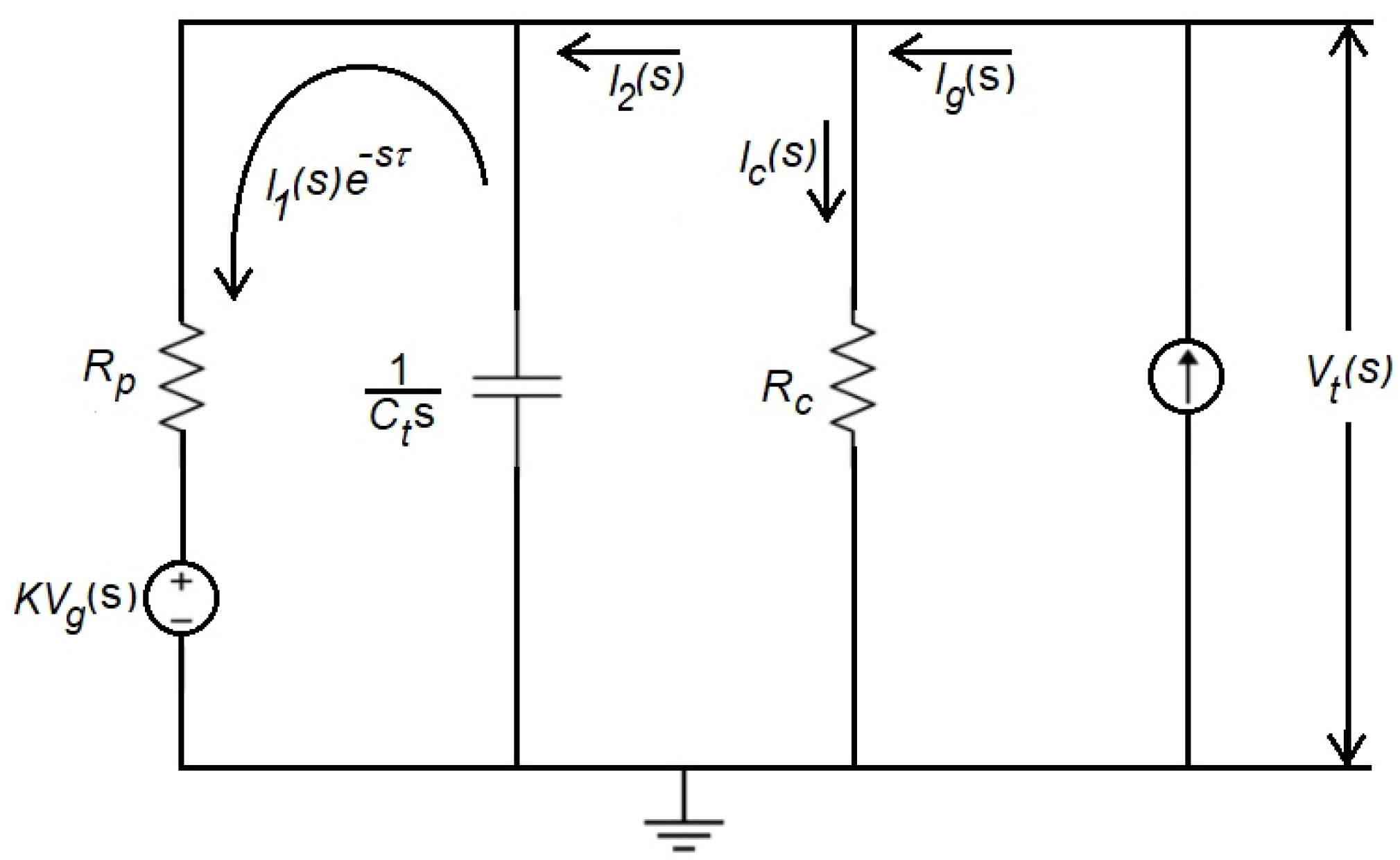
3.2. Model Considering a Delay to Represent the Transit of the Current through the Corona Triode
4. Terminal Voltage Regulation Problem
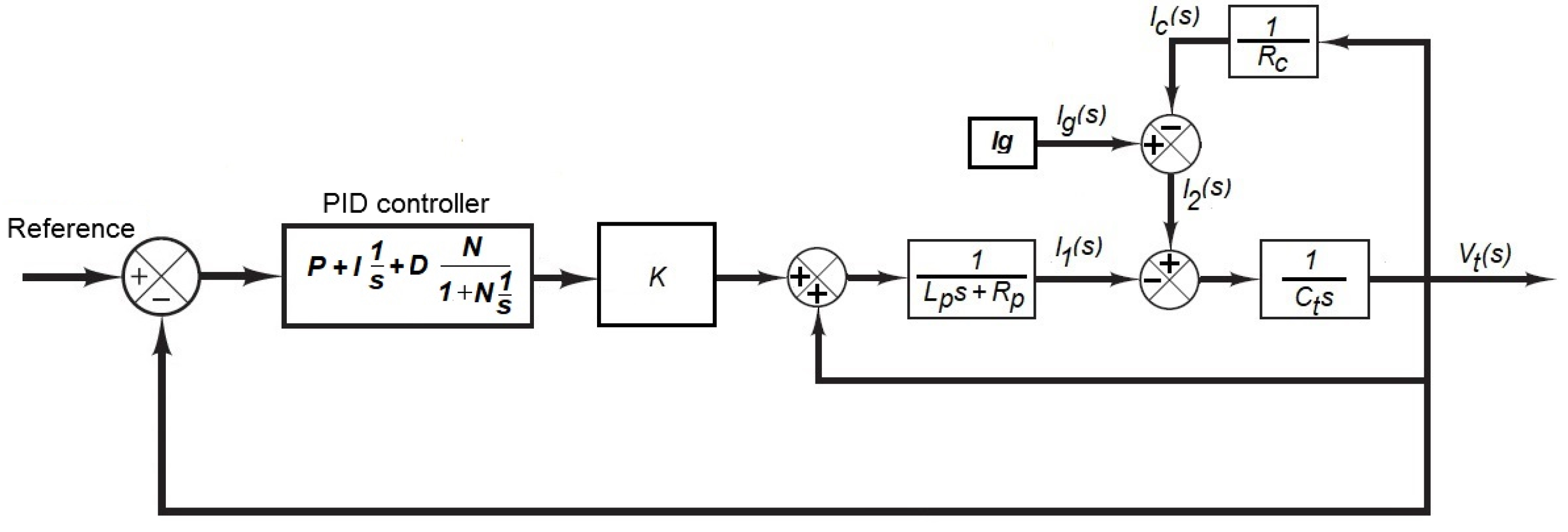
4.1. PID Controller
4.2. Sliding Mode Control
4.2.1. Time Domain Model of the Tandem Van de Graaff Accelerator Terminal
4.2.2. Sliding Mode Control Design
5. Conclusions
Author Contributions
Funding
Data Availability Statement
Conflicts of Interest
References
- Martínez Medina, M.A.; López Monroy, J.; Díaz Godoy, R.V.; Moreno Alcántara, J. Estudio espacial del carbono elemental presente en la fracción respirable de las PM2.5 mediante espectometría de retrodispersión de Rutherford en la zona metropolitana del Valler de Toluca. Rev. Int. Contam. Ambient. 2020, 36, 893–905. [Google Scholar]
- Gere, E.A. An Improved Control System for Van De Graaff Accelerators. IEEE Trans. Nucl. Sci. 1967, 14, 161–165. [Google Scholar] [CrossRef]
- Takacs, J. Corona Stabilizer for Van De Graaff Accelerators. Nucl. Instrum. Methods 1972, 103, 587–600. [Google Scholar] [CrossRef]
- Luthjens, L. Design and performance of control and long-term stabilization system for the IRI 3 MeV-Van de Graaff electron accelerator. Nucl. Instrum. Methods Phys. Res. A 2000, 455, 495–498. [Google Scholar] [CrossRef]
- Kansara, M.J.; Sapna, P.; Subrahmanyam, N.B.V.; Bhatt, J.P.; Singh, P. Development of a terminal voltage stabilization system for the FOTIA at BARC. PRAMANA—J. Phys. 2002, 59, 761–764. [Google Scholar] [CrossRef]
- Moşu, D.V.; Ghiţă, D.G.; Dobrescu, S.; Sava, T.; Mitu, I.O.; Călinescu, I.C.; Naghel, G.; Dumitru, G.; Căta-Danil, G. A new slit stabilization system for the beam energy at the Bucharest tandem Van de Graaff accelerator. Nucl. Instrum. Methods Phys. Res. A 2012, 963, 143–147. [Google Scholar] [CrossRef]
- Lobanov, N. Terminal Voltage Stabilization of Pelletron Tandem. In Proceedings of the HIAT, Chicago, IL, USA, 18–21 June 2012; pp. 125–128. [Google Scholar]
- Lobanov, N.R.; Linardakis, P.; Tsifakis, D. Development of a fast voltage control method for electrostatic accelerators. Nucl. Instrum. Methods Phys. Res. A 2014, 767, 433–438. [Google Scholar] [CrossRef]
- Bürger, W.; Lange, H.; Petr, V. A new method of improving the acceleration voltage stability of Van de Graaff accelerators. Nucl. Instrum. Methods Phys. Res. A 2008, 586, 160–168. [Google Scholar] [CrossRef]
- Mosu, D. Development of a GVM-based ion beam energy stabilization system at the Bucharest Van de Graaff FN tandem accelerator. Nucl. Instrum. Methods Phys. Res. A 2013, 707, 40–44. [Google Scholar] [CrossRef]
- Gonzalez, R. Van de Graaff Voltage Regulation via PID Control. In Proceedings of the 5th Joint Meeting of the APS Division of Nuclear Physics and the Physical Society of Japan, Waikoloa, HI, USA, 23–27 October 2018; Volume 63, pp. 75–89. [Google Scholar]
- Valerio-Lizarraga, C.A.; Duarte-Galvan, C.; Leon-Monzon, I.; Villasenor, P.; Aspiazu, J. A study on the negative ion beam production in the ININ sputtering ion source. Rev. Mex. FíSica 2019, 65, 278–283. [Google Scholar] [CrossRef]
- Mosu, D.; Ghita, D.; Sava, T.; Dobrescu, S.; Mitu, I.O.; Calinescu, I.C.; Savu, B.; Cata-Danil, G. Sensitivity of the ion beam focal position with respect to the terminal high voltage ripple in an FN-Tandem particle accelerator. Univ. Politeh. Buchar. Sci.-Bull.-Ser.-Appl. Math. Phys. 2013, 75, 207–214. [Google Scholar]
- Hinterberger, F. Electrostatic Accelerators. In CAS—CERN Accelerator School and KVI: Specialised CAS Course on Small Accelerators; Springer: Berlin/Heidelberg, Germany, 2006; pp. 95–112. [Google Scholar]
- Hellborg, R. Electrostatic Accelerators; Springer: Berlin/Heidelberg, Germany, 2005. [Google Scholar]
- Vermeer, A.; Strasters, B.A. The Corona Stabilization System of a Van De Graaff Generator. Nucl. Instrum. Methods 1978, 157, 427–440. [Google Scholar] [CrossRef]
- Willmott, C.J.; Matsuura, K. On the use of dimensioned measures of error to evaluate the performance of spatial interpolators. Int. J. Geogr. Inf. Sci. 2006, 20, 89–102. [Google Scholar] [CrossRef]
- Ugarte, R.; Álvarez, D.E. Simulación y Control de un Acelerador de Partículas. In Proceedings of the RPIC 2007—XII Reunión de Trabajo de Procesamiento de la Información y Control, Río Gallegos, Argentina, 16–18 October 2007; pp. 587–600. [Google Scholar]
- Sajnekar, D. Design of PID controller for automatic voltage regulator and validation using hardware in the loop technique. Int. J. Smart Grid Clean Energy 2018, 7, 75–89. [Google Scholar] [CrossRef]
- Herrera, M.; Camacho, O.; Leiva, H.; Smith, C. An approach of dynamic sliding mode control for chemical processes. J. Process Control 2020, 85, 112–120. [Google Scholar] [CrossRef]
- Saldivar, B. Sliding Mode Control for a Class of Control-Affine Nonlinear Systems. CEAI 2018, 20, 3–11. [Google Scholar]
- Shtessel, Y.; Edwards, C.; Fridman, L.; Levant, A. Sliding Mode Control and Observation; Springer: New York, NY, USA, 2014. [Google Scholar]
- Ding, Y.; Yan, X.G.; Mao, Z.; Jiang, B.; Spurgeon, S.K. Decentralized Sliding Mode Control for Output Tracking of Large-Scale Interconnected Systems. In Proceedings of the 60th IEEE Conference on Decision and Control (CDC), Austin, TX, USA, 13–17 December 2021; pp. 7094–7099. [Google Scholar]


| Distance | 20% | 30% | 40% | 50% | 60% | 70% | 80% | |
|---|---|---|---|---|---|---|---|---|
| Elements | ||||||||
| (H) | 8.5 × 10⁷ | 1.2 × 10⁸ | 1.4 × 10⁸ | 2.0 × 10⁸ | 2.6 × 10⁸ | 3.4 × 10⁸ | 4.6 × 10⁸ | |
| () | × | × | × | × | 3 × | × | × | |
| K | 4 × | × | × | × | × | × | × | |
| RMSE (Volts) | ||||||||
|---|---|---|---|---|---|---|---|---|
| Distance | 20% | 30% | 40% | 50% | 60% | 70% | 80% | |
| Model | ||||||||
| SICT | ||||||||
| Delayed | ||||||||
| Distance (%) | P (Proportional) | I (Integral) | D (Derivative) | N |
|---|---|---|---|---|
| 10 | 76 | 301 | 0.59 | 15 |
| 20 | 78 | 306 | 1.00 | 15 |
| 30 | 72 | 243 | 1.20 | 10 |
| 40 | 75 | 207 | 2.36 | 7 |
| 50 | 61 | 138 | 2.12 | 5 |
| 60 | 85 | 212 | 3.94 | 8 |
| 70 | 85 | 199 | 4.13 | 9 |
| 80 | 83 | 209 | 4.20 | 9 |
| 90 | 84 | 227 | 4.30 | 11 |
| RMSE (Volts) | ||||||||||
|---|---|---|---|---|---|---|---|---|---|---|
| Distance | 10% | 20% | 30% | 40% | 50% | 60% | 70% | 80% | 90% | |
| Controller | ||||||||||
| SMC | 652 | 660 | 1078 | 664 | 534 | 494 | 650 | 870 | 1014 | |
| PID | 171 | 151 | 167 | 200 | 205 | 314 | 438 | 541 | 580 | |
| Maximum Overshoot (Volts) | ||||||||||
|---|---|---|---|---|---|---|---|---|---|---|
| Distance | 10% | 20% | 30% | 40% | 50% | 60% | 70% | 80% | 90% | |
| Controller | ||||||||||
| SMC | none | none | none | none | none | none | none | none | none | |
| PID | 15 | 15 | 4400 | |||||||
| Settling Time (s) | ||||||||||
|---|---|---|---|---|---|---|---|---|---|---|
| Distance | 10% | 20% | 30% | 40% | 50% | 60% | 70% | 80% | 90% | |
| Controller | ||||||||||
| SMC | ||||||||||
| PID | ||||||||||
Disclaimer/Publisher’s Note: The statements, opinions and data contained in all publications are solely those of the individual author(s) and contributor(s) and not of MDPI and/or the editor(s). MDPI and/or the editor(s) disclaim responsibility for any injury to people or property resulting from any ideas, methods, instructions or products referred to in the content. |
© 2024 by the authors. Licensee MDPI, Basel, Switzerland. This article is an open access article distributed under the terms and conditions of the Creative Commons Attribution (CC BY) license (https://creativecommons.org/licenses/by/4.0/).
Share and Cite
Gutiérrez Ocampo, E.; Saldivar, B.; Ávila Vilchis, J.C.; Portillo-Rodríguez, O. Modeling and Control of the High-Voltage Terminal of a Tandem Van de Graaff Accelerator. Mathematics 2024, 12, 2335. https://doi.org/10.3390/math12152335
Gutiérrez Ocampo E, Saldivar B, Ávila Vilchis JC, Portillo-Rodríguez O. Modeling and Control of the High-Voltage Terminal of a Tandem Van de Graaff Accelerator. Mathematics. 2024; 12(15):2335. https://doi.org/10.3390/math12152335
Chicago/Turabian StyleGutiérrez Ocampo, Efrén, Belem Saldivar, Juan Carlos Ávila Vilchis, and Otniel Portillo-Rodríguez. 2024. "Modeling and Control of the High-Voltage Terminal of a Tandem Van de Graaff Accelerator" Mathematics 12, no. 15: 2335. https://doi.org/10.3390/math12152335
APA StyleGutiérrez Ocampo, E., Saldivar, B., Ávila Vilchis, J. C., & Portillo-Rodríguez, O. (2024). Modeling and Control of the High-Voltage Terminal of a Tandem Van de Graaff Accelerator. Mathematics, 12(15), 2335. https://doi.org/10.3390/math12152335