
Application of Extended Normal Distribution in Option Price Sensitivities


Abstract
:1. Introduction
2. Computation of Option Price under Extended Normal Distribution
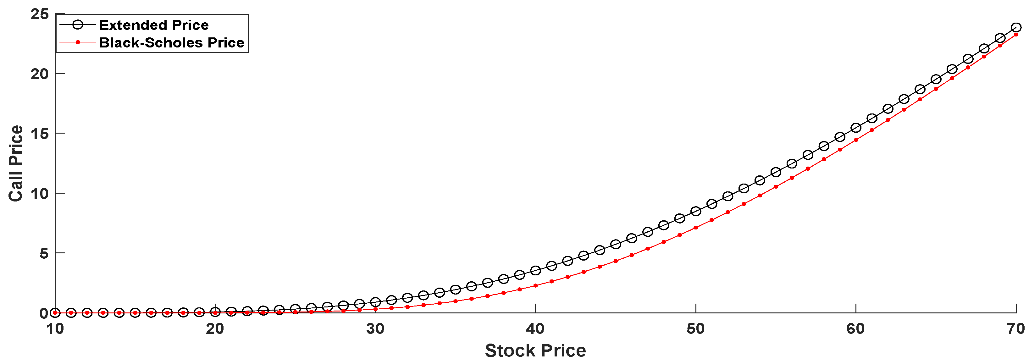
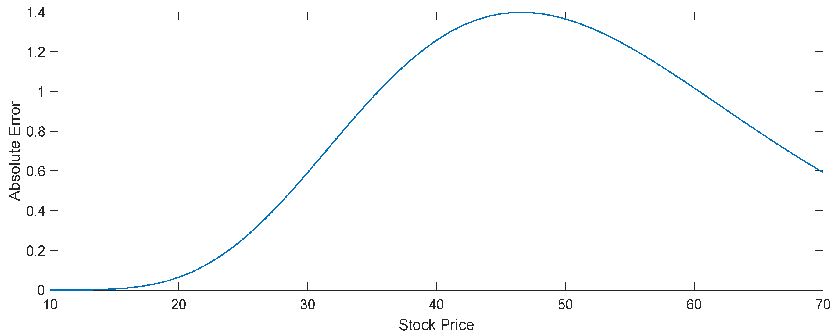
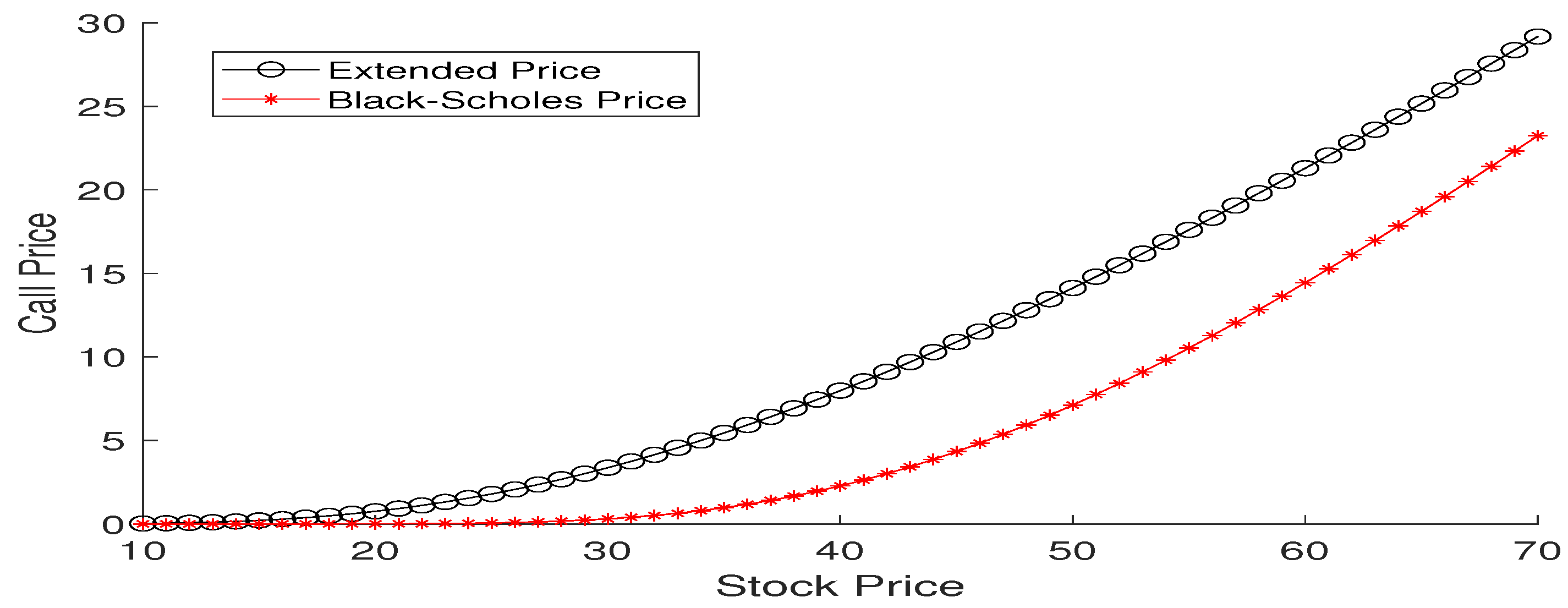
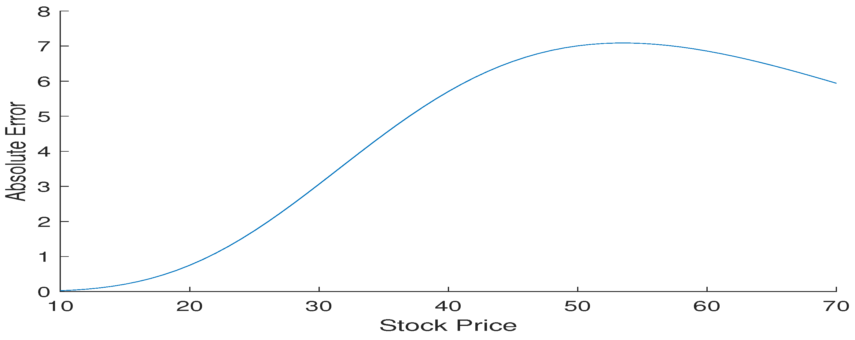
3. Graphical Interpretation
4. Computation of Option Greeks
- (i)
- Delta
- (ii)
- Gamma
- (iii)
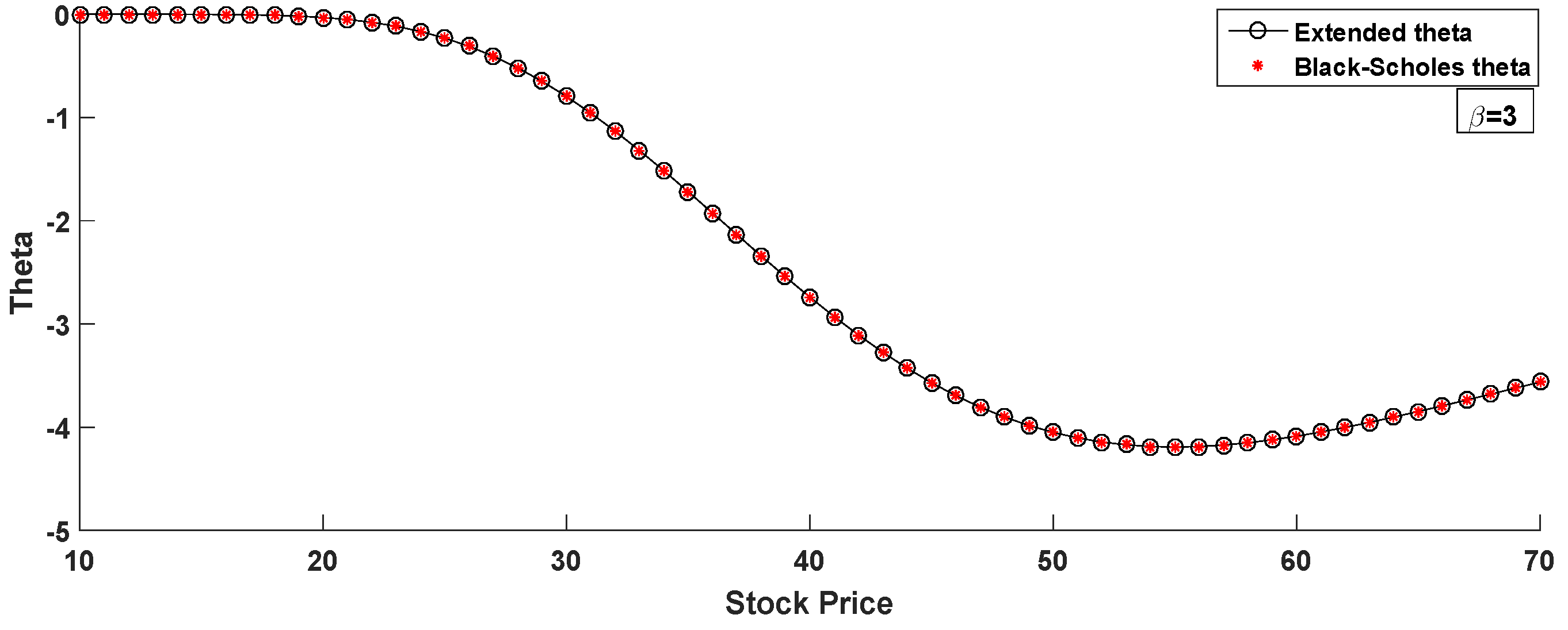
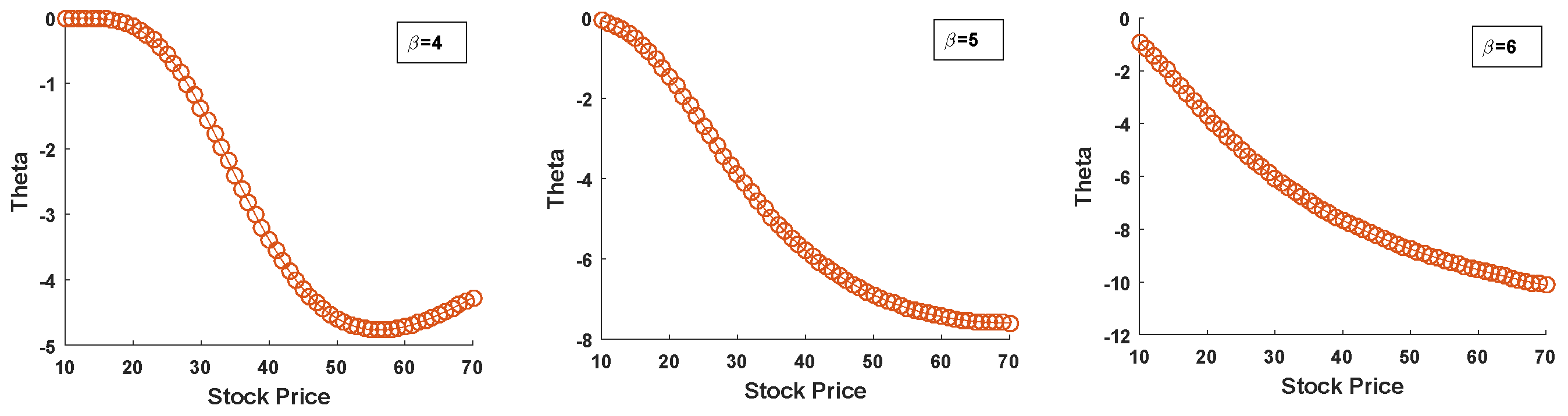
- Theta
- (iv)
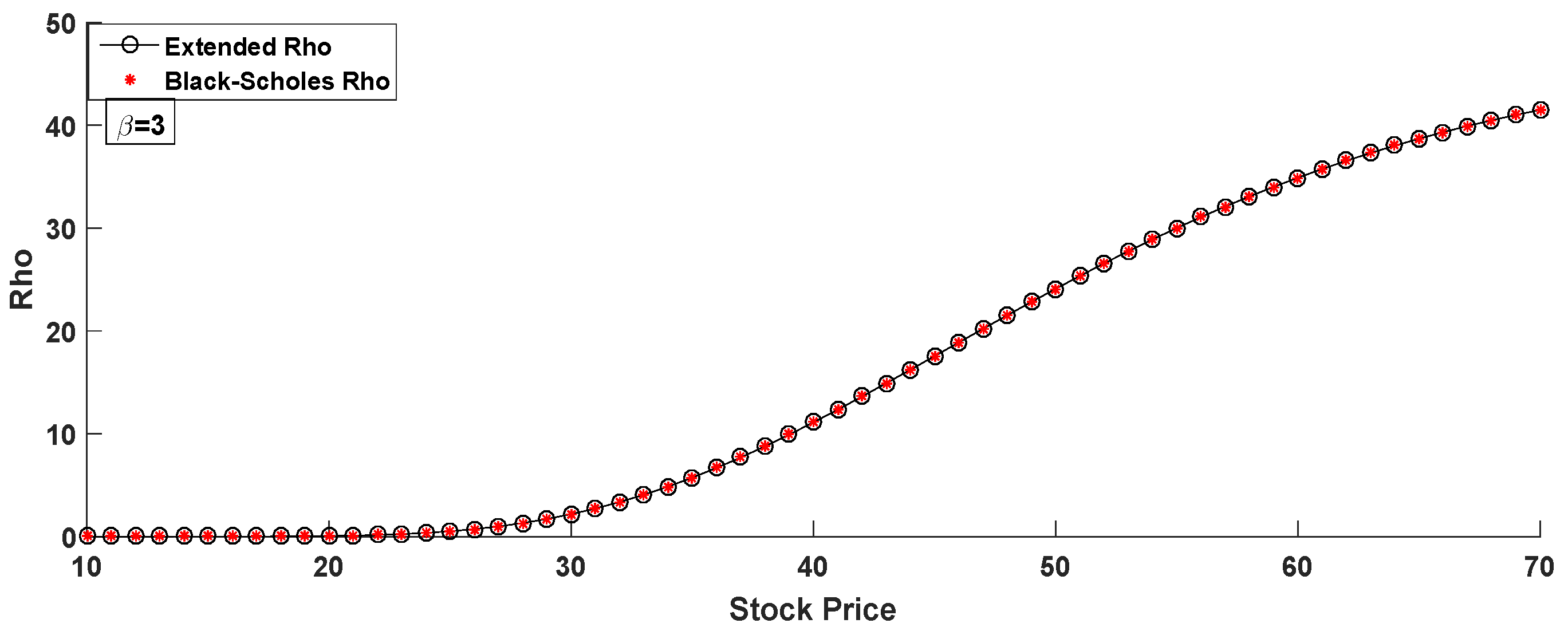
- Rho
- (v)
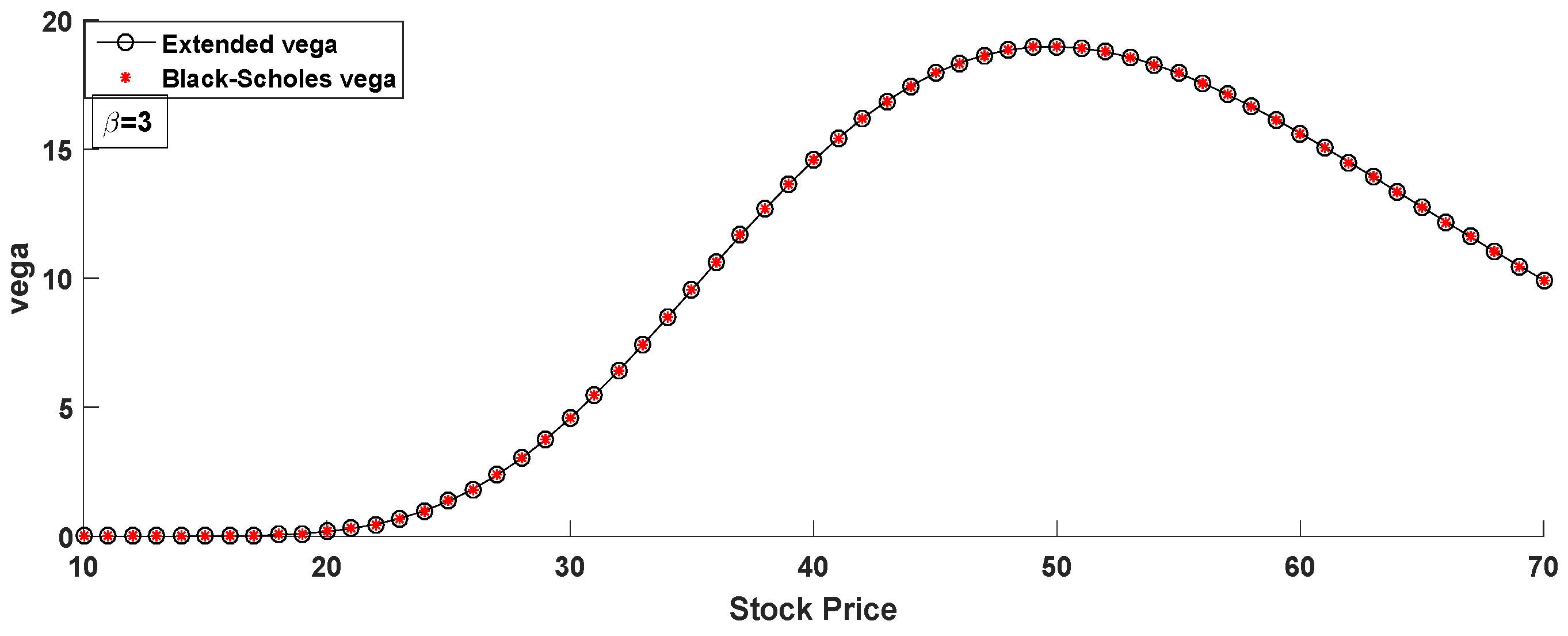
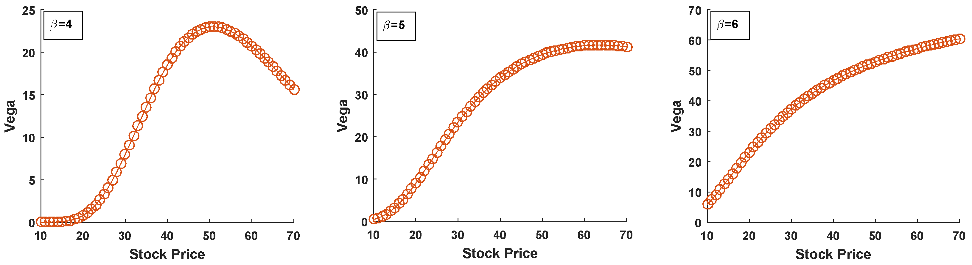
- Vega
- (vi)
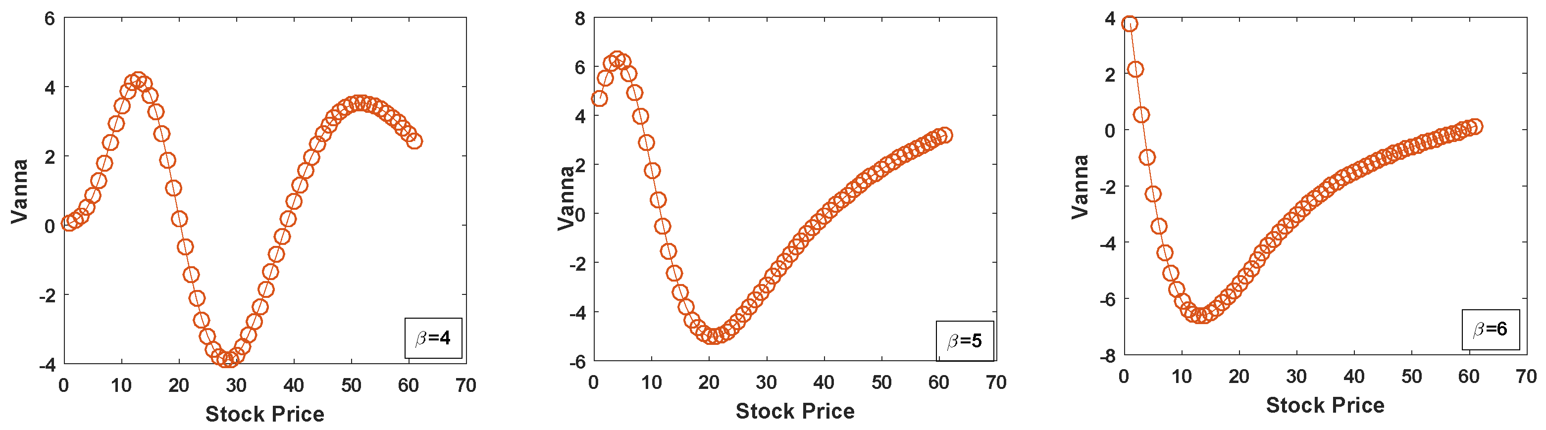
- Vanna
- (vii)
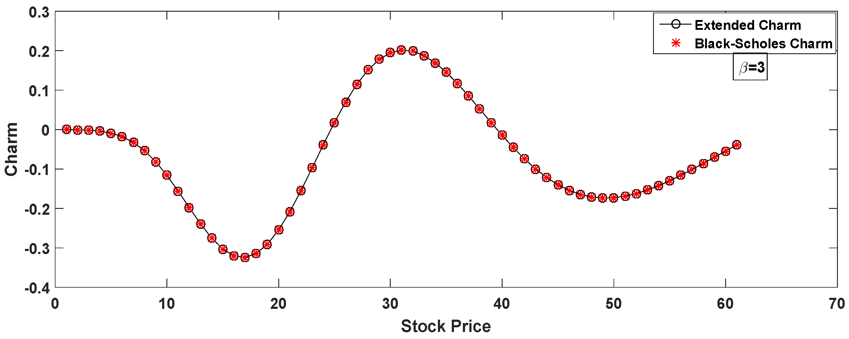
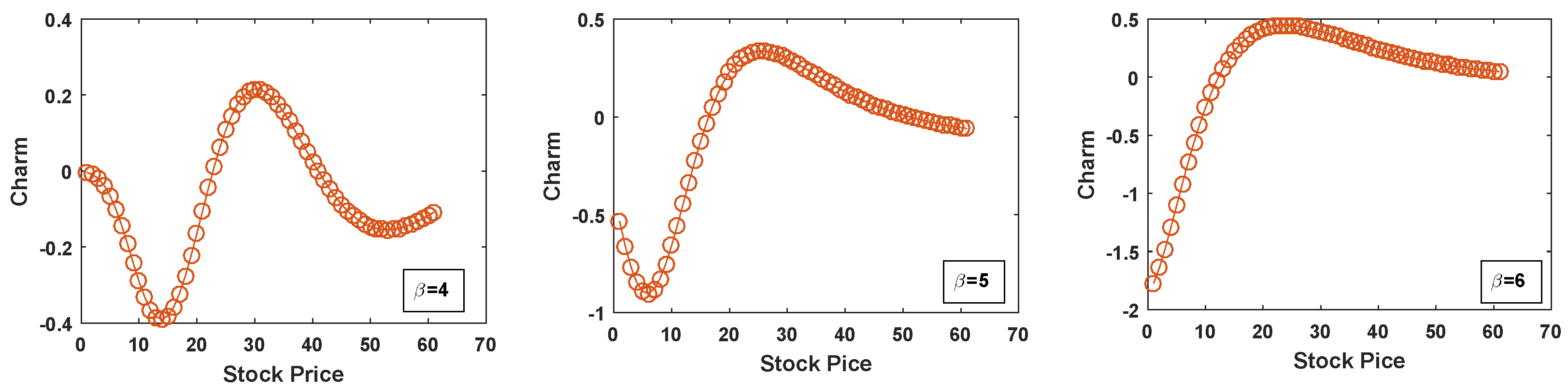
- Charm
- (viii)
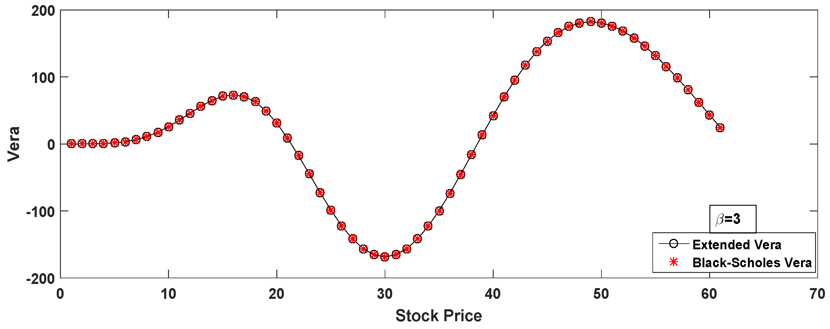
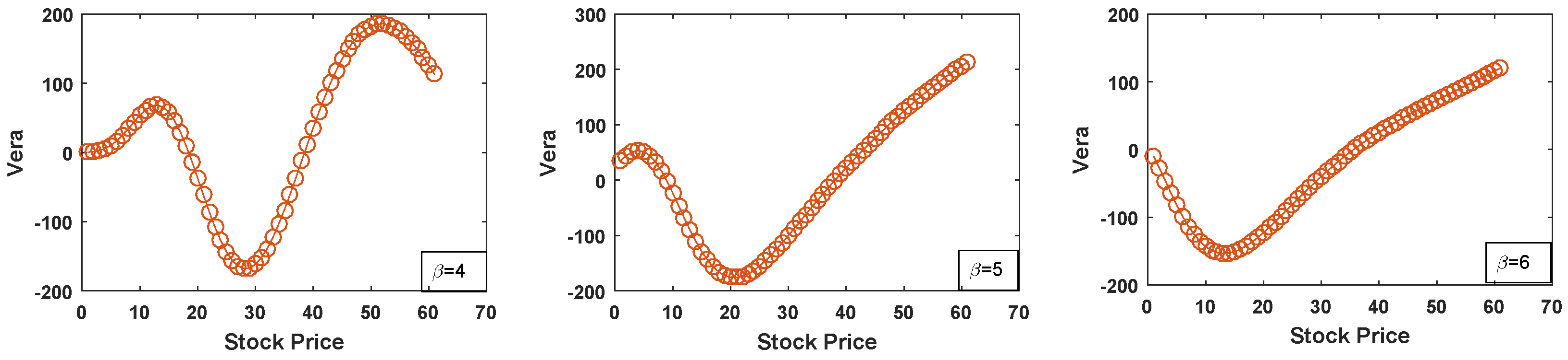
- Vera
5. Conclusions
Author Contributions
Funding
Data Availability Statement
Conflicts of Interest
References
- Black, F.; Scholes, M. The pricing of options and corporate liabilities. J. Political Econ. 1973, 81, 637–654. [Google Scholar] [CrossRef]
- Black, F. Fact and fantasy in the use of options. Financ. Anal. J. 1975, 31, 36–41. [Google Scholar] [CrossRef]
- MacBeth, J.D.; Merville, L.J. Tests of the Black-Scholes and Cox call option valuation models. J. Financ. 1980, 35, 285–301. [Google Scholar]
- Ki, H.; Choi, B.; Chang, K.H.; Lee, M. Option pricing under extended normal distribution. J. Futur. Mark. Futur. Options Other Deriv. Prod. 2005, 25, 845–871. [Google Scholar] [CrossRef]
- Karagiorgis, A.; Drakos, K. The Skewness-Kurtosis plane for non-Gaussian systems: The case of hedge fund returns. J. Int. Financ. Mark. Inst. Money 2022, 80, 101639. [Google Scholar] [CrossRef]
- Harris, R.D.; Coskun Küçüközmen, C. The empirical distribution of stock returns: Evidence from an emerging European market. Appl. Econ. Lett. 2001, 8, 367–371. [Google Scholar] [CrossRef]
- Fueki, T.; Hürtgen, P.; Walker, T.B. Zero-risk weights and capital misallocation. J. Financ. Stab. 2024, 72, 101264. [Google Scholar] [CrossRef]
- Pal, D. The distribution of commodity futures: A test of the generalized hyperbolic process. Appl. Econ. 2024, 56, 1763–1783. [Google Scholar] [CrossRef]
- Ahadzie, R.M.; Jeyasreedharan, N. Higher-order moments and asset pricing in the Australian stock market. Acc. Financ. 2024, 64, 75–128. [Google Scholar] [CrossRef]
- Bianchi, M.L.; Tassinari, G.L.; Fabozzi, F.J. Fat and Heavy Tails in Asset Management. J. Portf. Manag. 2023, 49, 236. [Google Scholar] [CrossRef]
- Necula, C.; Drimus, G.; Farkas, W. A general closed form option pricing formula. Rev. Deriv. Res. 2019, 22, 1–40. [Google Scholar] [CrossRef]
- Rubinstein, M. Edgeworth binomial trees. J. Deriv. 1998, 5, 20–27. [Google Scholar] [CrossRef]
- Heston, S.L. A closed-form solution for options with stochastic volatility with applications to bond and currency options. Rev. Financ. Stud. 1993, 6, 327–343. [Google Scholar] [CrossRef]
- Bakshi, G.; Cao, C.; Chen, Z. Empirical performance of alternative option pricing models. J. Financ. 1997, 52, 2003–2049. [Google Scholar] [CrossRef]
- Bibby, B.M.; Sørensen, M. A hyperbolic diffusion model for stock prices. Financ. Stochast. 1996, 1, 25–41. [Google Scholar] [CrossRef]
- Corrado, C.J.; Su, T. Skewness and kurtosis in S&P 500 index returns implied by option prices. J. Financ. Res. 1996, 19, 175–192. [Google Scholar]
- Li, F. Option pricing: How flexible should the SPD be? J. Deriv. 2000, 7, 49–65. [Google Scholar] [CrossRef]
- Jarrow, R.; Rudd, A. Approximate option valuation for arbitrary stochastic processes. J. Financ. Econ. 1982, 10, 347–369. [Google Scholar] [CrossRef]
- Cont, R. Empirical properties of asset returns: Stylized facts and statistical issues. Quant. Financ. 2001, 1, 223. [Google Scholar] [CrossRef]
- Ahn, K.; Choi, M.Y.; Dai, B.; Sohn, S.; Yang, B. Modeling stock return distributions with a quantum harmonic oscillator. EPL (Europhys. Lett.) 2018, 120, 38003. [Google Scholar] [CrossRef]
- Mwaniki, I.J. Modeling heteroscedastic, skewed and leptokurtic returns in discrete time. J. Appl. Financ. Bank. 2019, 9, 1–14. [Google Scholar]
- Wang, C.; Brunner, I.; Wang, J.; Guo, W.; Geng, Z.; Yang, X.; Chen, Z.; Han, S.; Li, M.H. The right-skewed distribution of fine-root size in three temperate forests in northeastern China. Front. Plant Sci. 2022, 12, 772463. [Google Scholar] [CrossRef] [PubMed]
- Bakshi, G.; Cao, C.; Zhong, Z. Assessing models of individual equity option prices. Rev. Quant. Financ. Acc. 2021, 57, 1–28. [Google Scholar] [CrossRef]
- Jurczenko, E.; Maillet, B.; Negrea, B. Skewness and Kurtosis Implied by Option Prices: A Second Comment; Financial Markets Group, The London School of Economics and Political Science: London, UK, 2002. [Google Scholar]
- Hull, J.C.; Basu, S. Options, Futures, and Other Derivatives; Pearson Education India: Bengaluru, India, 2016. [Google Scholar]
- Neftci, S.N. Principles of Financial Engineering; Academic Press: Cambridge, MA, USA, 2008. [Google Scholar]
- Leoni, P. The Greeks and Hedging Explained; Springer: Berlin/Heidelberg, Germany, 2014. [Google Scholar]
- Agrrawal, P. An automation algorithm for harvesting capital market information from the web. Manag. Financ. 2009, 35, 427–438. [Google Scholar]


| Delta | Gamma | Theta | |||||||
|---|---|---|---|---|---|---|---|---|---|
| Stock Price | |||||||||
| 51 | 0.6460 | 0.6836 | 0.7615 | 0.0199 | 0.0096 | 0.0054 | −4.6460 | −6.9710 | −8.8440 |
| 52 | 0.6655 | 0.6931 | 0.7699 | 0.0191 | 0.0092 | 0.0052 | −4.6900 | −7.0410 | −8.9300 |
| 53 | 0.6843 | 0.7021 | 0.7720 | 0.0183 | 0.0089 | 0.0050 | −4.7240 | −7.1070 | −9.0140 |
| 54 | 0.7022 | 0.7109 | 0.7770 | 0.0175 | 0.0085 | 0.0048 | −4.7480 | −7.1670 | −9.0960 |
| 55 | 0.7194 | 0.7193 | 0.7817 | 0.0167 | 0.0082 | 0.0046 | −4.7620 | −7.2230 | −9.1750 |
| 56 | 0.7358 | 0.7275 | 0.7863 | 0.0152 | 0.0077 | 0.0044 | −4.7680 | −7.2740 | −9.2520 |
| 57 | 0.7514 | 0.7353 | 0.7907 | 0.0144 | 0.0074 | 0.0041 | −4.7660 | −7.3210 | −9.3260 |
| 58 | 0.7662 | 0.7429 | 0.7949 | 0.0137 | 0.0072 | 0.0040 | −4.7560 | −7.3640 | −9.3980 |
| 59 | 0.7803 | 0.7502 | 0.7990 | 0.0130 | 0.0069 | 0.0038 | −4.7400 | −7.4020 | −9.4690 |
| 60 | 0.7937 | 0.7573 | 0.8030 | 0.0123 | 0.0067 | 0.0037 | −4.7170 | −7.4370 | −9.5370 |
| 61 | 0.8064 | 0.7642 | 0.8067 | 0.0098 | 0.0051 | 0.0032 | −4.6890 | −7.4680 | −9.6030 |
| Rho | Vega | Vanna | |||||||
|---|---|---|---|---|---|---|---|---|---|
| Stock Price | |||||||||
| 51 | 23.99 | 20.16 | 16.81 | 22.98 | 39.75 | 53.35 | 3.518 | 1.965 | −0.541 |
| 52 | 24.99 | 20.64 | 17.09 | 22.94 | 40.06 | 53.84 | 3.525 | 2.114 | −0.470 |
| 53 | 25.98 | 21.12 | 17.36 | 22.83 | 40.34 | 54.31 | 3.498 | 2.257 | −0.401 |
| 54 | 26.94 | 21.59 | 17.62 | 22.67 | 40.59 | 54.77 | 3.441 | 2.394 | −0.334 |
| 55 | 22.46 | 40.80 | 55.21 | 22.46 | 40.80 | 55.21 | 3.355 | 2.526 | −2.267 |
| 56 | 28.78 | 22.50 | 18.14 | 22.19 | 41.00 | 55.63 | 3.245 | 2.652 | −0.201 |
| 57 | 29.66 | 22.94 | 18.39 | 21.88 | 41.16 | 56.05 | 3.115 | 2.772 | −0.135 |
| 58 | 30.52 | 23.38 | 18.63 | 21.54 | 41.30 | 56.46 | 2.962 | 2.885 | −0.070 |
| 59 | 31.34 | 23.81 | 18.87 | 21.15 | 41.44 | 56.83 | 2.797 | 2.993 | −0.005 |
| 60 | 32.14 | 24.23 | 19.10 | 20.73 | 41.50 | 57.21 | 2.618 | 3.095 | −0.058 |
| 61 | 32.90 | 24.64 | 19.33 | 20.29 | 41.57 | 57.58 | 2.43 | 3.190 | −0.122 |
| Charm | Vera | |||||
|---|---|---|---|---|---|---|
| Stock Price | ||||||
| 51 | −0.151 | 0.001 | 0.113 | 185.4 | 134.1 | 77.11 |
| 52 | −0.154 | −0.006 | 0.105 | 185.9 | 143.1 | 81.36 |
| 53 | −0.154 | −0.013 | 0.097 | 184.2 | 151.9 | 85.60 |
| 54 | −0.153 | −0.020 | 0.089 | 180.6 | 160.5 | 89.84 |
| 55 | −0.150 | −0.027 | 0.082 | 175.2 | 168.8 | 94.09 |
| 56 | −0.146 | −0.033 | 0.075 | 168.0 | 176.9 | 98.35 |
| 57 | −0.140 | −0.039 | 0.069 | 159.4 | 184.8 | 102.6 |
| 58 | −0.133 | −0.045 | 0.063 | 149.4 | 192.6 | 107.0 |
| 59 | −0.126 | −0.050 | 0.057 | 138.2 | 199.6 | 111.3 |
| 60 | −0.117 | −0.055 | 0.052 | 126.0 | 206.6 | 115.7 |
| 61 | −0.108 | −0.059 | 0.047 | 112.9 | 213.2 | 120.2 |
Disclaimer/Publisher’s Note: The statements, opinions and data contained in all publications are solely those of the individual author(s) and contributor(s) and not of MDPI and/or the editor(s). MDPI and/or the editor(s) disclaim responsibility for any injury to people or property resulting from any ideas, methods, instructions or products referred to in the content. |
© 2024 by the authors. Licensee MDPI, Basel, Switzerland. This article is an open access article distributed under the terms and conditions of the Creative Commons Attribution (CC BY) license (https://creativecommons.org/licenses/by/4.0/).
Share and Cite
Nayak, G.; Tripathy, S.S.; Imoize, A.L.; Li, C.-T. Application of Extended Normal Distribution in Option Price Sensitivities. Mathematics 2024, 12, 2346. https://doi.org/10.3390/math12152346
Nayak G, Tripathy SS, Imoize AL, Li C-T. Application of Extended Normal Distribution in Option Price Sensitivities. Mathematics. 2024; 12(15):2346. https://doi.org/10.3390/math12152346
Chicago/Turabian StyleNayak, Gangadhar, Subhranshu Sekhar Tripathy, Agbotiname Lucky Imoize, and Chun-Ta Li. 2024. "Application of Extended Normal Distribution in Option Price Sensitivities" Mathematics 12, no. 15: 2346. https://doi.org/10.3390/math12152346