A Predator–Prey System with a Modified Leslie–Gower and Prey Stage Structure Scheme in Deterministic and Stochastic Environments

Abstract

The evolution of the population ecosystem is closely related to resources and the environment. Assuming that the environmental capacity of a predator population is positively correlated with the number of prey, and that the prey population has a sheltered effect, we investigated a predator–prey model with a juvenile–adult two-stage structure. The dynamical behaviour of the model was examined from two distinct environmental perspectives, deterministic and stochastic, respectively. For the deterministic model, the conditions for the existence of equilibrium points were obtained by comprehensive use of analytical and geometric methods, and the local and global asymptotic stability of each equilibrium point was discussed. For the stochastic system, the effect of noise intensity on the long-term dynamic behavior of the population was investigated. By constructing appropriate Lyapunov functions, the criteria that determined the extinction of the system and the ergodic stationary distribution were given. Finally, through concrete examples and numerical simulations, the understanding of the dynamic properties of the model was deepened. The results show that an improvement in the predator living environment would lead to the decrease in the prey population, while more prey shelters could lead to the decline or even extinction of predator populations.

1. Introduction

“Survival of the fittest” is the basic law of species evolution in nature. In order to adapt to the living environment, each species has evolved its own internal population growth mode and generation replacement mechanism. The logistic model regards environmental capacity as a constant; however, the environmental capacity of many species is related to the amount of food they depend on in their habitat, rather than being constant. In 1948, Leslie et al. [1,2] assumed that the environmental capacity of a predator is proportional to the abundance of surrounding food, and constructed the following model—the classic Leslie–Gower predator–prey model

$$\left\{\begin{array}{c}{\displaystyle \frac{\mathrm{d}x\left(t\right)}{\mathrm{d}t}=(r_1-b_{1}x\left(t\right))x\left(t\right)-p\left(x\left(t\right)\right)y\left(t\right),}\hfill \\ {\displaystyle \frac{\mathrm{d}y\left(t\right)}{\mathrm{d}t}=\left(r_2-a_2\frac{y\left(t\right)}{x\left(t\right)}\right)y\left(t\right),}\hfill \end{array}\right.$$

(1)

where $x\left(t\right)$, $y\left(t\right)$ denote the densities of the prey and predator populations in the environment at time t, respectively. $r_1$, $r_2$ are the intrinsic growth rate of the prey and predator populations, respectively; ${\displaystyle \frac{a_{2}y\left(t\right)}{x\left(t\right)}}$ is the Leslie–Gower term; and $p\left(x\right)$ is the functional response function. From the first equation of model (1), it is easy to see that, in the absence of predators, the prey population grows logistically. From the second equation of model (1), the environmental carrying capacity of the predator is ${\displaystyle \frac{r_{2}x\left(t\right)}{a_2}}$. The Leslie predation model has been widely used in the study of various ecosystems [3,4,5,6]. In 1988, David J. Wollkind et al. [3] put forward a mite predation model with the Leslie term and Holling-II functional response when they were studying the control of fruit tree pests using Typhlodromus occidentalis, a natural enemy of mites, and discussed the dependence of ecosystem stability on environmental temperature. Li et al. [7] constructed a mite predation model using a simplified Holling-IV functional response function and investigated the bifurcation dynamic behavior of the system. When the living environment of a biological population changes dramatically, such as the change of autumn and winter seasons and climate drought, the food preferred by predators may decrease sharply during a certain period of time. In the case of severe food shortage, predators may have to turn to other substitute prey in order to survive. In this case, Aziz-Alaoui and Nindjin et al. [8,9] revised the Leslie term to ${\displaystyle \frac{ay\left(t\right)}{h+x\left(t\right)}}$, where h is the substitutable quantity of predator’s favorite food, which reflects the protective effect of the environment on predators. By coupling the modified Leslie–Gower term into the model (1), Aziz-Alaoui et al. [9] studied the boundedness and global stability of the following model.

$$\left\{\begin{array}{c}{\displaystyle \frac{\mathrm{d}x\left(t\right)}{\mathrm{d}t}=(r_1-b_{1}x\left(t\right)-\frac{a_{1}y\left(t\right)}{x\left(t\right)+k_1})x\left(t\right),}\hfill \\ {\displaystyle \frac{\mathrm{d}y\left(t\right)}{\mathrm{d}t}=\left(r_2-\frac{a_{2}y\left(t\right)}{x\left(t\right)+k_2}\right)y\left(t\right),}\hfill \end{array}\right.$$

(2)

here, $k_1$ and $k_2$ are used to measure the degree of environmental protection for the prey and predator, respectively. Many ecosystems in nature, such as the insect(pest)–spider food chain, can support model (2), see [10,11]. Puchuri et al. [12] replaced the Holling-II functional response function ${\displaystyle \frac{a_{1}x}{x+k_1}}$ in system (2) with the Holling-IV functional response function $p\left(x\right)={\displaystyle \frac{ax}{r+x^2}}$, which established a kind of mite predation model, and discussed the multi-stability of the system.

As is known to all, species have different life characteristics at different stages of their life cycle. Cubs in the initial stage of life are generally infertile, weak in predation and defense, and mainly rely on their parents to feed and shelter them. Adult individuals at the peak stage of their life cycle are mature and have strong predation ability, and bear the heavy responsibility of reproducing while maintaining their own survival. In order to describe the population characteristics in different life stages in detail, the biological population model with stage structure is widely used in various ecosystem studies [13,14,15,16,17,18,19]. Zhang et al. [14] constructed a predation model of a prey population with a two-stage structure of juvenile–adult, and studied the dynamic properties of the system and the optimal harvesting strategy. In this model, the predator is supposed only to prey on juvenile prey and the predation rate is the Holling-I functional response. A predator–prey model with both the stage structure of prey and the Crowley–Martin functional response is considered by Maiti et al. [15]. Here, the authors assume that the predator only preys on adult prey. Based on [14,15], Zhang et al. constructed the following food chain model with a two-stage structure of prey in [16].

$$\left\{\begin{array}{c}{\displaystyle \frac{\mathrm{d}x}{\mathrm{d}t}=ry-mx-\alpha xz-d_{1}x,}\hfill \\ {\displaystyle \frac{\mathrm{d}y}{\mathrm{d}t}=mx-s{y}^2-\frac{\beta yz}{(1+ay)(1+bz)}-d_{2}y,}\hfill \\ {\displaystyle \frac{\mathrm{d}z}{\mathrm{d}t}=p\alpha xz+\frac{q\beta yz}{(1+ay)(1+bz)}-\delta z^2-d_{3}z,}\hfill \end{array}\right.$$

(3)

where the predator z feeds on both juvenile x and adult y prey, with predation rates of $\alpha x$ (Holling-I) and ${\displaystyle \frac{\beta y}{(1+ay)(1+bz)}}$ (Crowley–Martin-type), respectively. The conclusion suggests that system (3) may not only have multiple positive equilibrium points, but also exhibit rich dynamical properties such as bistability and complex branching.

In order to adapt to the harsh natural environment, many animals have evolved special survival skills. For example, chameleons conceal themselves by blending into their surroundings, groundhogs dig holes in the ground to serve as shelters, and swarms of bees increase the efficiency of their defences by dividing up their work. Animals can effectively reduce the predation efficiency of predators by using shelters and group defense, so that they can gain greater chances of survival in front of predators, and then gain advantages in the process of evolution. It is generally believed that prey refuge has two important functions: preventing the extinction of prey populations and inhibiting the oscillation of the predator–prey system [20,21]. Jamil et al. [22] constructed a modified Leslie–Gower model with prey refuge and fear effects, and investigated the rich dynamical behaviors of the system including bi-stability. There are many ways to couple the prey refuge into the predator–prey model [23,24,25]. Xiang et al. [23] set the refuge effect as a constant (denoted as $\mu$). If the prey population is lower than the amount $\mu$, the predator cannot catch the prey, but if the prey population is higher than $\mu$, the predator can catch the prey. The author found that constant prey refuge can prevent the extinction of prey and lead to global coexistence. Zhang et al. [24] assumed the probability of the prey population obtaining shelter is $\nu (0<\nu <1)$, thus reducing the predation rate of predators per unit time. Referring to the method of introducing shelter in [24], this paper constructs the following food chain model with the modified Leslie–Gower term and prey stage structure.

$$\left\{\begin{array}{c}{\displaystyle \frac{\mathrm{d}x\left(t\right)}{\mathrm{d}t}=r_{1}y-gx-b{x}^2-d_{1}x,}\hfill \\ {\displaystyle \frac{\mathrm{d}y\left(t\right)}{\mathrm{d}t}=gx-f{y}^2-d_{2}y-\frac{\beta (1-\nu )yz}{1+k(1-\nu )y},}\hfill \\ {\displaystyle \frac{\mathrm{d}z\left(t\right)}{\mathrm{d}t}=z\left(\frac{c\beta (1-\nu )y}{1+k(1-\nu )y}-\frac{r_{2}z}{h+y}\right)-d_{3}z,}\hfill \end{array}\right.$$

(4)

with initial value:

$$x\left(0\right)=x_0>0,y\left(0\right)=y_0>0,z\left(0\right)=z_0>0,$$

(5)

where $x\left(t\right)$, $y\left(t\right)$, and $z\left(t\right)$ represent the densities of juvenile prey, adult prey, and predator, respectively, at time t. The model supposes that the predator only preys on adult prey, where $\nu (0<\nu <1)$ is the probability of obtaining shelter for adult prey, and other parameters are positive constants and their biological significances are shown in Table 1.

Table 1. Biological interpretations of parameters.

Parameter	Biological Interpretation
$r_1$	The birth rate of juvenile prey
$r_2$	The maximum value of per capita reduction rate of adult prey
b	Intra-specific competition coefficient of juvenile prey
g	Conversion rate of prey from juvenile to adult
$d_1$	Natural mortality rate of juvenile prey
$d_2$	Natural mortality rate of adult prey
$d_3$	Natural mortality rate of predator
f	Intra-specific competition coefficient of adult prey
$\beta$	Capture rate
$\nu$	Strength of prey refuge
k	Half-saturation parameter
c	Conversion efficiency of predator
h	Degree of environmental improvement

In addition, environmental disturbance is very important for the development and evolution of population ecosystems [26,27,28,29]. Considering random interference factors, white noise is coupled into model (4), and the following stochastic system is obtained

$$\left\{\begin{array}{c}{\displaystyle \mathrm{d}x=(r_{1}y-b{x}^2-gx-d_{1}x)dt+{\sigma }_{1}x\mathrm{d}{B}_1\left(t\right),}\hfill \\ {\displaystyle \mathrm{d}y=\left(gx-f{y}^2-d_{2}y-\frac{\beta (1-\nu )yz}{1+k(1-\nu )y}\right)dt+{\sigma }_{2}y\mathrm{d}{B}_2\left(t\right),}\hfill \\ {\displaystyle \mathrm{d}z=\left(z\left(\frac{c\beta (1-\nu )y}{1+k(1-\nu )y}-\frac{r_{2}z}{h+y}\right)-d_{3}z\right)dt+{\sigma }_{3}z\mathrm{d}{B}_3\left(t\right),}\hfill \end{array}\right.$$

(6)

where ${\sigma }_i^2(i=1,2,3)$ represent the intensity of white noise and $B_i\left(t\right)$ are the independent standard Brownian motion.

In this paper, we focus on the dynamic behavior of a predator–prey model in two different environments. For the deterministic model (4), Part 2 discusses the model’s well-posedness, the existence of equilibrium points, and the local and global asymptotic stability. For the stochastic model (6) under the disturbance of environmental noise, the adequacy criterion for determining the extinction and existence of ergodic stationary distribution is given in Part 3. In the fourth part, the theoretical results are numerically simulated, while in the fifth part, the relevant conclusions of this paper are presented.

2. Dynamics of Deterministic System (4)

Firstly, the well-posedness of the solution of system (4) is discussed.

Theorem 1. 

For any given initial condition (5), there exists a unique solution to the system (4), and the solution is non-negative and uniformly bounded.

Proof. 

Let $X\left(t\right)={\left(x\right(t),y(t),z(t\left)\right)}^{\mathrm{T}}$ be any solution of the system (4). We rewrite the right side of system (4) as follows:

$$\begin{array}{c}\hfill F\left(X\right)=\left[\begin{array}{c}{\displaystyle F_1\left(X\right)}\\ {\displaystyle F_2\left(X\right)}\\ {\displaystyle F_3\left(X\right)}\end{array}\right]=\left[\begin{array}{c}{\displaystyle r_{1}y-gx-b{x}^2-d_{1}x}\\ {\displaystyle gx-f{y}^2-d_{2}y-\frac{\beta (1-\nu )yz}{1+k(1-\nu )y}}\\ {\displaystyle z\left(\frac{c\beta (1-\nu )y}{1+k(1-\nu )y}-\frac{r_{2}z}{h+y}\right)-d_{3}z}\end{array}\right].\end{array}$$

Define

$$V\left(t\right)=x\left(t\right)+cy\left(t\right)+z\left(t\right),$$

then

$$\begin{array}{cc}\hfill {\displaystyle \frac{\mathrm{d}V}{\mathrm{d}t}}=& -b{x}^2+(c-1)gx-cf{y}^2+r_{1}y-{\displaystyle \frac{r_2{z}^2}{h+y}}-d_{1}x-c{d}_{2}y-d_{3}z\hfill \\ \hfill & \le \overline{H}-dV\left(t\right),\hfill \end{array}$$

where

$$\overline{H}:=max\left\{-b{x}^2+(c-1)gx-cf{y}^2+r_{1}y\right\}={\displaystyle \frac{{(c-1)}^2{g}^2}{4b}}+{\displaystyle \frac{r_1^2}{4cf}},d=min\left\{d_1,d_2,d_3\right\}.$$

Based on the above analysis, we have

$$\underset{t\to \infty }{\lim \sup } V\left(t\right)\le {\displaystyle \frac{\overline{H}}{d}}={\displaystyle \frac{{(c-1)}^2{g}^2}{4bd}}+{\displaystyle \frac{r_1^2}{4cfd}},$$

therefore, any solution to (4) with an initial value of (5) will eventually approach or remain in the area

$$\Omega =\left\{(x,y,z)\in {\mathbb{R}}_{+}^3:0\le x\left(t\right)+cy\left(t\right)+z\left(t\right)\le {\displaystyle \frac{\overline{H}}{d}}\right\}.$$

On account of ${\displaystyle \frac{dX}{dt}}{|}_{X=0}\ge 0$, therefore, any solution to the system (4) is non-negative.

Next, we prove that $F:{\mathbb{R}}^3\to {\mathbb{R}}^3$, satisfying the local Lipschitz condition [30].

Let $X={(x\left(t\right),y\left(t\right),z\left(t\right))}^T$ and $\overline{X}={(\overline{x}\left(t\right),\overline{y}\left(t\right),\overline{z}\left(t\right))}^T$ be two arbitrary solutions of system (4), then, we have

$$\begin{array}{cc}\hfill \parallel & F\left(X\right)-F\left(\overline{X}\right)\parallel \hfill \\ \hfill =& |F_1\left(X\right)-F_1\left(\overline{X}\right)|+|F_2\left(X\right)-F_2\left(\overline{X}\right)|+|F_3\left(X\right)-F_3\left(\overline{X}\right)|\hfill \\ \hfill =& |r_1(y-\overline{y})-(g+d_1)(x-\overline{x})-b(x+\overline{x})(x-\overline{x})|\hfill \\ & +\left|g(x-\overline{x})-f(y+\overline{y})(y-\overline{y})-d_2(y-\overline{y})-\beta (1-\nu ){\displaystyle \frac{yz+k(1-\nu )y\overline{y}z-\overline{y}\overline{z}-k(1-\nu )y\overline{y}\overline{z}}{(1+k(1-\nu )y)(1+k(1-\nu )\overline{y})}}\right|\hfill \\ & +\left|c\beta (1-\nu )\left({\displaystyle \frac{yz}{1+k(1-\nu )y}}-{\displaystyle \frac{\overline{y}\overline{z}}{1+k(1-\nu )\overline{y}}}\right)-r_2\left({\displaystyle \frac{z^2}{h+y}}-{\displaystyle \frac{{\overline{z}}^2}{h+\overline{y}}}\right)-d_3(z-\overline{z})\right|.\hfill \end{array}$$

Using the boundedness of system (4), it is obtained

$$\begin{array}{cc}\hfill \parallel & F\left(X\right)-F\left(\overline{X}\right)\parallel \hfill \\ \hfill \le & r_1|y-\overline{y}|+\left(g+d_1+{\displaystyle \frac{2b\overline{H}}{d}}\right)|x-\overline{x}|+g|x-\overline{x}|+\left({\displaystyle \frac{2f\overline{H}}{cd}}+d_2+{\displaystyle \frac{\overline{H}\beta (1-\nu )}{d}}\right)|y-\overline{y}|\hfill \\ & +{\displaystyle \frac{\overline{H}\beta (1-\nu )}{cd}}|z-\overline{z}|+\left({\displaystyle \frac{c\beta (1-\nu )\overline{H}}{d}}+{\displaystyle \frac{r_2{\overline{H}}^2}{h^2{d}^2}}\right)|y-\overline{y}|+\left({\displaystyle \frac{\beta (1-\nu )\overline{H}}{d}}+{\displaystyle \frac{2r_2\overline{H}}{hd}}+d_3\right)|z-\overline{z}|\hfill \\ \hfill =& \left(2g+d_1+{\displaystyle \frac{2b\overline{H}}{d}}\right)|x-\overline{x}|+\left(r_1+d_2+{\displaystyle \frac{2f\overline{H}}{cd}}+{\displaystyle \frac{\overline{H}\beta (1+c)(1-\nu )}{d}}+{\displaystyle \frac{r_2{\overline{H}}^2}{h^2{d}^2}}\right)|y-\overline{y}|\hfill \\ & +\left(d_3+{\displaystyle \frac{\beta (1+c)(1-\nu )\overline{H}}{cd}}+{\displaystyle \frac{2r_2\overline{H}}{hd}}\right)|z-\overline{z}|\hfill \\ \hfill \le & L\parallel X-\overline{X}\parallel .\hfill \end{array}$$

where

$$\begin{array}{c}\hfill L=max\left\{2g+d_1+{\displaystyle \frac{2b\overline{H}}{d}},r_1+d_2+{\displaystyle \frac{2f\overline{H}}{cd}}+{\displaystyle \frac{\overline{H}\beta (1+c)(1-\nu )}{d}}+{\displaystyle \frac{r_2{\overline{H}}^2}{h^2{d}^2}},\right.\\ \hfill \phantom{=}\left.d_3+{\displaystyle \frac{\beta (1+c)(1-\nu )\overline{H}}{cd}}+{\displaystyle \frac{2r_2\overline{H}}{hd}}\right\}.\end{array}$$

Consequently, the mapping $F\left(X\right)$ satisfies the local Lipschitz condition. Thus, for any given initial condition (5), there exists a unique solution to the system (4).    □

Subsequently, the existence and stability of the equilibrium point of the system (4) are investigated. Making the right side of (4) equal to zero provides the following equations:

$$r_{1}y-gx-b{x}^2-d_{1}x=0,$$

(7)

$$gx-f{y}^2-d_{2}y-{\displaystyle \frac{\beta (1-\nu )yz}{1+k(1-\nu )y}}=0,$$

(8)

$$z\left({\displaystyle \frac{c\beta (1-\nu )y}{1+k(1-\nu )y}}-{\displaystyle \frac{r_{2}z}{h+y}}\right)-d_{3}z=0.$$

(9)

Clearly, there exists a trivial equilibrium point $E_0:(0,0,0)$ for the system (4). Transforming (7), we obtain

$$y={\displaystyle \frac{x}{r_1}}(bx+g+d_1).$$

(10)

Define

$$R_0={\displaystyle \frac{r_{1}g}{d_2(g+d_1)}}.$$

(11)

The existence of nontrivial equilibrium of the model is discussed below in two cases.

Case I.

$z=0$.

In this case, by substituting (10) into (8), we have

$$f{b}^2{x}^3+2fb(g+d_1)x^2+(f{(g+d_1)}^2+r_{1}b{d}_2)x+r_1{d}_2(g+d_1)-r_1^{2}g=0.$$

(12)

Using the Cartesian symbol criterion [31], when $R_0>1$, Equation (12) has a unique positive root $\check{x}$. Therefore, $\check{y}={\displaystyle \frac{\check{x}}{r_1}}(b\check{x}+g+d_1)$, subsequently, there exists a unique boundary equilibrium $\check{E}:(\check{x},\check{y},0)$ for the system (4).

Case II.

$z\ne 0$.

It is vital to solve Equations (7)–(9) in order to find the positive equilibrium point of system (4). Substitute (10) into (8) and (9), we have

$$G_1(x,z)=0,G_2(x,z)=0,$$

where

$$G_1(x,z)=g-{\displaystyle \frac{d_2}{r_1}}(bx+g+d_1)-{\displaystyle \frac{\beta (1-\nu )(bx+g+d_1)z}{r_1+k(1-\nu )x(bx+g+d_1)}}-{\displaystyle \frac{fx{(bx+g+d_1)}^2}{r_1^2}},$$

$$G_2(x,z)=-{\displaystyle \frac{r_1{r}_{2}z}{r_{1}h+x(bx+g+d_1)}}+{\displaystyle \frac{c\beta (1-\nu )(bx+g+d_1)x}{r_1+k(1-\nu )x(bx+g+d_1)}}-d_3.$$

As shown in Figure 1, the intersection of curve $G_1(x,z)=0$ with the coordinate axis of $(0,z_1)$, $(\check{x},0)$, here $z_1={\displaystyle \frac{r_{1}g-d_2(g+d_1)}{\beta (1-\nu )(g+d_1)}}$, $\check{x}$, is the root of Equation (12). Obviously, if $R_0>1$, then $z_1>0$ holds.

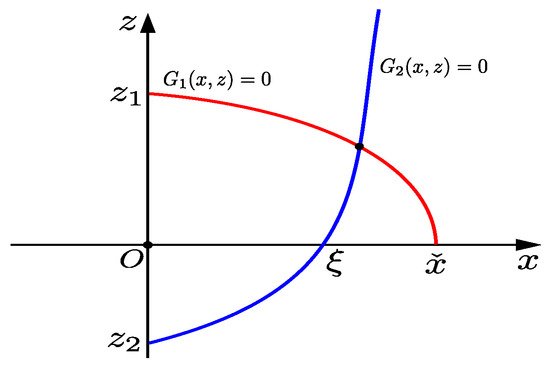
Figure 1. Schematic representation of curves $G_1(x,z)=0,G_2(x,z)=0$.

Suppose that the implicit function determined by equation $G_2(x,z)=0$ is $z=H\left(x\right)$, it is known that ${\displaystyle \frac{dz}{dx}}=-{\displaystyle \frac{\frac{\partial G_2}{\partial x}}{\frac{\partial G_2}{\partial z}}}>0$, thus, $z=H\left(x\right)$ is monotonically increasing. From $G_2(0,z)=0$, we know the intersection of curve $G_2(x,z)=0$ with the z-axis is $(0,z_2)$; here, $z_2=-{\displaystyle \frac{h{d}_3}{r_2}}$. From $G_2(x,0)=0$, we know when $c\beta >k{d}_3$, the intersection of curve $G_2(x,z)=0$ with the x-axis is $(\xi ,0)$, where $\xi ={\displaystyle \frac{-(g+d_1)+\sqrt{{(g+d_1)}^2+\frac{4b{d}_3{r}_1}{(c\beta -d_{3}k)(1-\nu )}}}{2b}}$. If $\xi <\check{x}$, curves $G_1(x,z)=0$ and $G_2(x,z)=0$ have at least one intersection point $(x^{*},z^{*})$ in the first quadrant. So, if $R_0>1$, $c\beta >k{d}_3$, and $\xi <\check{x}$, we can say that there is at least one positive equilibrium $E^{*}:(x^{*},y^{*},z^{*})$ in system (4); here, $y^{*}={\displaystyle \frac{x^{*}}{r_1}}(b{x}^{*}+g+d_1)$.

Based on the above discussion, the equilibrium points of model (4) can be obtained as follows

Theorem 2. 

(1) There always exists a trivial equilibrium point $E_0:(0,0,0)$.

(2) If $R_0>1$ holds, then there exists a unique boundary equilibrium point $\check{E}:(\check{x},\check{y},0)$.

(3) If $R_0>1$, $c\beta >k{d}_3$, and $\xi <\check{x}$ hold simultaneously, then there exists at least one positive equilibrium point $E^{*}:(x^{*},y^{*},z^{*})$, where $\xi ={\displaystyle \frac{-(g+d_1)+\sqrt{{(g+d_1)}^2+\frac{4b{d}_3{r}_1}{(1-\nu )(c\beta -k{d}_3)}}}{2b}}$.

The stability of each equilibrium point is discussed below. The Jacobian matrix corresponding to system (4) is

$$\begin{array}{c}\hfill J=\left(\begin{array}{cccc}{\displaystyle -2bx-g-d_1}& {\displaystyle r_1}& {\displaystyle 0}& {\displaystyle }\\ g& {\displaystyle -d_2-2fy-\frac{\beta (1-\nu )z}{{(1+k(1-\nu )y)}^2}}& {\displaystyle -\frac{\beta (1-\nu )y}{1+k(1-\nu )y}}& \\ {\displaystyle 0}& {\displaystyle \frac{r_2{z}^2}{{(h+y)}^2}+\frac{c\beta (1-\nu )z}{{(1+k(1-\nu )y)}^2}}& -{\displaystyle \frac{2r_{2}z}{h+y}}+{\displaystyle \frac{c\beta (1-\nu )y}{1+k(1-\nu )y}}-d_3& \end{array}\right).\end{array}$$

By substituting each equilibrium point into the above matrix and using the Routh–Hurwitz criterion [32], we can obtain

Theorem 3. 

(1) If $R_0<1$ holds, $E_0:(0,0,0)$ of system (4) is locally asymptotically stable.

(2) If $R_0>1$, $r_{1}g<(2b\check{x}+g+d_1)(d_2+2f\check{y})$ and $d_3>{\displaystyle \frac{c\beta (1-\nu )\check{y}}{1+k(1-\nu )\check{y}}}$ hold, $\check{E}:(\check{x},\check{y},0)$ is locally asymptotically stable.

(3) If $R_0>1$, $0<\xi <\check{x}$ and $\left[Q_1\right],\left[Q_2\right]\left[Q_3\right]$ hold, then $E^{*}:(x^{*},y^{*},z^{*})$ is locally asymptotically stable, where $\left[Q_i\right](i=1,2,3)$ are defined by (15)–(17).

Proof. 

(1) The Jacobian matrix corresponding to $E_0:(0,0,0)$ is

$$\begin{array}{c}\hfill {\left.J\right|}_{E_0}=\left(\begin{array}{cccc}{\displaystyle -g-d_1}& {\displaystyle r_1}& {\displaystyle 0}& {\displaystyle }\\ g& {\displaystyle -d_2}& {\displaystyle 0}& \\ {\displaystyle 0}& {\displaystyle 0}& -d_3& \end{array}\right),\end{array}$$

and its characteristic equation is expressed as follows

$$(\lambda +d_3)({\lambda }^2+(d_2+d_1+g)\lambda +d_2(g+d_1)-r_{1}g)=0.$$

From the above equation, we have

$${\lambda }_1=-d_3<0,{\lambda }_{2,3}={\displaystyle \frac{-(d_2+g+d_1)\pm \sqrt{{(d_2+g+d_1)}^2-4(d_{2}g+d_2{d}_1-r_{1}g)}}{2}}.$$

If $R_0<1$ holds, we can easily obtain ${\lambda }_1,{\lambda }_2,{\lambda }_3<0$, which means $E_0$ is locally asymptotically stable. Conversely, if $R_0>1$, $E_0$ is unstable.

(2) Similarly, substituting the coordinates of the equilibrium point $\check{E}:(\check{x},\check{y},0)$ into J, we can obtain

$$\begin{array}{c}\hfill {\left.J\right|}_{\check{E}}=\left(\begin{array}{cccc}{\displaystyle -2b\check{x}-g-d_1}& {\displaystyle r_1}& {\displaystyle 0}& {\displaystyle }\\ g& {\displaystyle -d_2-2f\check{y}}& {\displaystyle -\frac{\beta (1-\nu )\check{y}}{1+k(1-\nu )\check{y}}}& \\ {\displaystyle 0}& {\displaystyle 0}& {\displaystyle \frac{c\beta (1-\nu )\check{y}}{1+k(1-\nu )\check{y}}}-d_3& \end{array}\right).\end{array}$$

The corresponding characteristic equation is

$$\begin{array}{cc}\hfill & \left(\lambda +d_3-{\displaystyle \frac{c\beta (1-\nu )\check{y}}{1+k(1-\nu )\check{y}}}\right)\begin{array}{c}\hfill ({\lambda }^2+(2b\check{x}+g+d_1+d_2+2f\check{y})\lambda \end{array}\hfill \\ & +(2b\check{x}+g+d_1)(d_2+2f\check{y})-r_{1}g)=0,\hfill \end{array}$$

and the eigenvalues are solved as

$${\lambda }_1={\displaystyle \frac{c\beta (1-\nu )\check{y}}{1+k(1-\nu )\check{y}}}-d_3,{\lambda }_{2,3}={\displaystyle \frac{-l_1\pm \sqrt{l_1^2-4l_2}}{2}},$$

where $l_1=2b\check{x}+g+d_1+d_2+2f\check{y}$, $l_2=(2b\check{x}+g+d_1)(d_2+2f\check{y})-r_{1}g$. So, when $\check{E}$ exists, and the conditions

$$d_3>{\displaystyle \frac{c\beta (1-\nu )\check{y}}{1+k(1-\nu )\check{y}}}$$

and

$$r_{1}g<(2b\check{x}+g+d_1)(d_2+2f\check{y})$$

are met, we can easily obtain ${\lambda }_{1,2,3}<0$; to clarify, $\check{E}:(\check{x},\check{y},0)$ is locally asymptotically stable.

(3) At the equilibrium point $E^{*}:(x^{*},y^{*},z^{*})$, the Jacobian matrix may be found as

$${\left.J\right|}_{E^{*}}=\left(\begin{array}{cccc}{\displaystyle -2b{x}^{*}-g-d_1}& {\displaystyle r_1}& {\displaystyle 0}& {\displaystyle }\\ g& {\displaystyle -d_2-2f{y}^{*}-\frac{\beta (1-\nu )z^{*}}{{(1+k(1-\nu )y^{*})}^2}}& {\displaystyle -\frac{\beta (1-\nu )y^{*}}{1+k(1-\nu )y^{*}}}& \\ {\displaystyle 0}& {\displaystyle \frac{r_2{z^{*}}^2}{{(h+y^{*})}^2}+\frac{c\beta (1-\nu )z^{*}}{{(1+k(1-\nu )y^{*})}^2}}& -{\displaystyle \frac{2r_2{z}^{*}}{h+y^{*}}}+{\displaystyle \frac{c\beta (1-\nu )y^{*}}{1+k(1-\nu )y^{*}}}-d_3& \end{array}\right),$$

and its characteristic equation is

$${\lambda }^3+(A_1+A_2+A_3){\lambda }^2+(A_1{A}_2+A_1{A}_3+A_2{A}_3+B-r_{1}g)\lambda +A_1{A}_2{A}_3+A_{1}B-A_3{r}_{1}g=0,$$

where

$$A_1=2b{x}^{*}+g+d_1,A_2=d_2+2f{y}^{*}+{\displaystyle \frac{\beta (1-\nu )z^{*}}{{(1+k(1-\nu )y^{*})}^2}},A_3={\displaystyle \frac{2r_2{z}^{*}}{h+y^{*}}}-{\displaystyle \frac{c\beta (1-\nu )y^{*}}{1+k(1-\nu )y^{*}}}+d_3,$$

(13)

$$B=\left({\displaystyle \frac{r_2{z^{*}}^2}{{(h+y^{*})}^2}}+{\displaystyle \frac{c\beta (1-\nu )z^{*}}{{(1+k(1-\nu )y^{*})}^2}}\right){\displaystyle \frac{\beta (1-\nu )y^{*}}{1+k(1-\nu )y^{*}}}.$$

(14)

From Routh–Hurwitz criteria, when

$$\left[Q_1\right]:A_1+A_2+A_3>0,$$

(15)

$$\left[Q_2\right]:A_1{A}_2{A}_3+A_{1}B-A_3{r}_{1}g>0,$$

(16)

$$\left[Q_3\right]:(A_1{A}_2-r_{1}g)(A_1+A_2)+A_1{A}_3(A_1+A_3)+(A_2{A}_3+B)(A_2+A_3)+2A_1{A}_2{A}_3>0,$$

(17)

$E^{*}:(x^{*},y^{*}$, $z^{*})$ is locally asymptotically stable.    □

Lemma 1 

([33] Lyapunov’s stability theorem). For an autonomous system

$$\left\{\begin{array}{c}{\displaystyle \frac{dX\left(t\right)}{dt}=f\left(X\right),}\hfill \\ f\left(0\right)=0,\hfill \end{array}\right.$$

if there is a function $V:R^n\to R$ satisfies:

(1) 

$V\left(X\right)$ is continuous together with its first partial derivatives;

(2) 

$V\left(X\right)$ is positive definite, that is $V\left(X\right)\ge 0$, $V\left(0\right)=0$, if and only if, $X=0$;

(3) 

$V\left(X\right)$ is radially unbounded, namely, if $\parallel X\parallel \to \infty$, then $V\left(x\right)\to \infty$;

(4) 

${\displaystyle \frac{dV\left(X\right(t\left)\right)}{dt}}$ is negative definite, that is, for $\forall X\in R^n\setminus \left\{0\right\}$, there is ${\displaystyle \frac{dV}{dt}}={\displaystyle \frac{\partial V}{\partial X}}·{\displaystyle \frac{dX}{dt}}<0$,

then the equilibrium point $X=0$ is globally asymptotically stable.

Theorem 4. 

Assume $\check{E}:(\check{x},\check{y},0)$ is locally asymptotically stable and satisfies $c\beta <k{d}_3$, then $\check{E}:(\check{x},\check{y},0)$ is globally asymptotically stable.

Proof. 

Obviously, the boundary equilibrium $\check{E}:(\check{x},\check{y},0)$ satisfies

$$\left\{\begin{array}{c}{\displaystyle \frac{r_1\check{y}}{\check{x}}-b\check{x}-g-d_1=0,}\hfill \\ {\displaystyle \frac{g\check{x}}{\check{y}}-f\check{y}-d_2=0.}\hfill \end{array}\right.$$

We define the Lyapunov function

$$V(x,y,z)=\check{k_1}(x-\check{x}-\check{x}\ln {\displaystyle \frac{x}{\check{x}}})+\check{k_2}(y-\check{y}-\check{y}\ln {\displaystyle \frac{y}{\check{y}}})+\check{k_3}z,$$

where $\check{k_1},\check{k_2},\check{k_3}$ are positive constants. Following this, we compute that

$$\begin{array}{cc}\hfill {\displaystyle \frac{\mathrm{d}V}{\mathrm{d}t}}=& \check{k_1}(1-{\displaystyle \frac{\check{x}}{x}})(r_{1}y-b{x}^2-gx-d_{1}x)\hfill \\ \hfill & +\check{k_2}(1-{\displaystyle \frac{\check{y}}{y}})\left(gx-d_{2}y-{\displaystyle \frac{\beta (1-\nu )yz}{1+k(1-\nu )y}}-f{y}^2\right)\hfill \\ \hfill & +\check{k_3}\left(-{\displaystyle \frac{r_2{z}^2}{h+y}}+{\displaystyle \frac{c\beta (1-\nu )yz}{1+k(1-\nu )y}}-d_{3}z\right)\hfill \\ \hfill =& \check{k_1}(x-\check{x})\left({\displaystyle \frac{r_{1}y}{x}}-{\displaystyle \frac{r_1\check{y}}{\check{x}}}+b(\check{x}-x)\right)\hfill \\ \hfill & +k_2(y-\check{y})\left({\displaystyle \frac{gx}{y}}-{\displaystyle \frac{g\check{x}}{\check{y}}}-{\displaystyle \frac{\beta (1-\nu )z}{1+k(1-\nu )y}}+f(\check{y}-y)\right)\hfill \\ \hfill & +\check{k_3}z\left(-{\displaystyle \frac{r_{2}z}{h+y}}+{\displaystyle \frac{c\beta (1-\nu )y}{1+k(1-\nu )y}}-d_3\right)\hfill \\ \hfill =& -b\check{k_1}{(x-\check{x})}^2-{\displaystyle \frac{\check{k_1}{r}_1{(x-\check{x})}^{2}y}{x\check{x}}}+{\displaystyle \frac{\check{k_1}{r}_1(x-\check{x})(y-\check{y})}{\check{x}}}\hfill \\ \hfill & -{\displaystyle \frac{k_{2}g{(y-\check{y})}^{2}x}{y\check{y}}}+{\displaystyle \frac{\check{k_2}g(y-\check{y})(x-\check{x})}{\check{y}}}-{\displaystyle \frac{\check{k_2}\beta (1-\nu )yz}{1+k(1-\nu )y}}\hfill \\ \hfill & +{\displaystyle \frac{\beta (1-\nu )(\check{k_2}\check{y}z+\check{k_3}cyz)}{1+k(1-\nu )y}}-{\displaystyle \frac{r_2\check{k_3}{z}^2}{h+y}}-d_3\check{k_3}z-f\check{k_2}{(y-\check{y})}^2.\hfill \end{array}$$

Let $\check{k_1}={\displaystyle \frac{\check{x}}{r_1}},\check{k_2}={\displaystyle \frac{\check{y}}{g}}$, we have

$$\begin{array}{cc}\hfill & -{\displaystyle \frac{\check{k_1}{r}_1{(x-\check{x})}^{2}y}{x\check{x}}}+{\displaystyle \frac{\check{k_1}{r}_1(x-\check{x})(y-\check{y})}{\check{x}}}-{\displaystyle \frac{\check{k_2}g{(y-\check{y})}^{2}x}{y\check{y}}}+{\displaystyle \frac{\check{k_2}g(y-\check{y})(x-\check{x})}{\check{y}}}\hfill \\ \hfill =& -{\left(\sqrt{{\displaystyle \frac{y}{x}}}(x-\check{x})-\sqrt{{\displaystyle \frac{x}{y}}}(y-\check{y}))\right)}^2\hfill \\ \hfill \le & 0,\hfill \end{array}$$

then

$${\displaystyle \frac{\mathrm{d}V}{\mathrm{d}t}}\le -{\displaystyle \frac{b\check{x}}{r_1}}{(x-\check{x})}^2-{\displaystyle \frac{f\check{y}}{g}}{(y-\check{y})}^2+\left(\check{k_2}\beta (1-\nu )\check{y}+{\displaystyle \frac{\check{k_3}c\beta }{k}}-\check{k_3}{d}_3\right)z.$$

When $c\beta -d_{3}k<0$, choose $\check{k_3}>{\displaystyle \frac{k\beta (1-\nu ){\check{y}}^2}{g(d_{3}k-c\beta )}}$, and we obtain ${\displaystyle \frac{\mathrm{d}V}{\mathrm{d}t}}\le 0.$ Therefore, if $\check{E}:(\check{x},\check{y},0)$ is locally asymptotically stable and the condition

$$c\beta -d_{3}k<0$$

is met, then $\check{E}:(\check{x},\check{y},0)$ is globally asymptotically stable.    □

With the aim of discussing the global stability of the positive equilibrium point $E^{*}:(x^{*},y^{*},z^{*})$ of model (4), the assumption is given that

$$\left[H_1\right]:f>{\displaystyle \frac{k\beta {(1-\nu )}^2{z}^{*}}{1+k(1-\nu )y^{*}}}+{\displaystyle \frac{r_2(1+k(1-\nu )y^{*}){z^{*}}^2}{4ch{(h+y^{*})}^2}}.$$

Theorem 5. 

Assume $E^{*}:(x^{*},y^{*},z^{*})$ is local asymptotically stable and $\left[H_1\right]$ holds, then $E^{*}:(x^{*},y^{*},z^{*})$ is globally asymptotically stable.

Proof. 

At the interior equilibrium $E^{*}:(x^{*},y^{*},z^{*})$, we have

$$\left\{\begin{array}{c}{\displaystyle \frac{r_1{y}^{*}}{x^{*}}-b{x}^{*}-g-d_1=0,}\hfill \\ {\displaystyle \frac{g{x}^{*}}{y^{*}}-\frac{\beta (1-\nu )z^{*}}{1+k(1-\nu )y^{*}}-f{y}^{*}-d_2=0,}\hfill \\ {\displaystyle -\frac{r_2{z}^{*}}{h+y^{*}}+\frac{c\beta (1-\nu )y^{*}}{1+k(1-\nu )y^{*}}-d_3=0.}\hfill \end{array}\right.$$

Define the Lyapunov function

$$V(x,y,z)=k_1^{*}(x-x^{*}-x^{*}\ln {\displaystyle \frac{x}{x^{*}}})+k_2^{*}(y-y^{*}-y^{*}\ln {\displaystyle \frac{y}{y^{*}}})+k_3^{*}(z-z^{*}-z^{*}\ln {\displaystyle \frac{z}{z^{*}}}).$$

Then, there is

$$\begin{array}{cc}\hfill {\displaystyle \frac{\mathrm{d}V}{\mathrm{d}t}}=& k_1^{*}(1-{\displaystyle \frac{x^{*}}{x}})(r_{1}y-b{x}^2-gx-d_{1}x)\hfill \\ & +k_2^{*}(1-{\displaystyle \frac{y^{*}}{y}})\left(gx-d_{2}y-{\displaystyle \frac{\beta (1-\nu )yz}{1+k(1-\nu )y}}-f{y}^2\right)\hfill \\ & +k_3^{*}(1-{\displaystyle \frac{z^{*}}{z}})\left(-{\displaystyle \frac{r_2{z}^2}{h+y}}+{\displaystyle \frac{c\beta (1-\nu )yz}{1+k(1-\nu )y}}-d_{3}z\right)\hfill \\ \hfill =& k_1^{*}(x-x^{*})\left(r_1\left({\displaystyle \frac{y}{x}}-{\displaystyle \frac{y^{*}}{x^{*}}}\right)+b(x^{*}-x)\right)\hfill \\ & \left.+k_2^{*}(y-y^{*})\left(g\left({\displaystyle \frac{x}{y}}-{\displaystyle \frac{x^{*}}{y^{*}}}\right)+f(y^{*}-y)\right.+\beta (1-\nu )\left({\displaystyle \frac{z^{*}}{1+k(1-\nu )y^{*}}}-{\displaystyle \frac{z}{1+k(1-\nu )y}}\right)\right)\hfill \\ & +k_3^{*}(z-z^{*})\left(r_2\left({\displaystyle \frac{z^{*}}{h+y^{*}}}-{\displaystyle \frac{z}{h+y}}\right)+c\beta (1-\nu )\left({\displaystyle \frac{y}{1+k(1-\nu )y}}-{\displaystyle \frac{y^{*}}{1+k(1-\nu )y^{*}}}\right)\right)\hfill \\ \hfill =& -b{k}_1^{*}{(x-x^{*})}^2-{\displaystyle \frac{k_1^{*}{r}_1{(x-x^{*})}^{2}y}{x{x}^{*}}}+{\displaystyle \frac{k_1^{*}{r}_1(x-x^{*})(y-y^{*})}{x^{*}}}-{\displaystyle \frac{k_2^{*}g{(y-y^{*})}^{2}x}{y{y}^{*}}}\hfill \\ & +{\displaystyle \frac{k_2^{*}g(y-y^{*})(x-x^{*})}{y^{*}}}+{\displaystyle \frac{(k_3^{*}c-k_2^{*}-k_2^{*}k(1-\nu )y^{*})\beta (1-\nu )(y-y^{*})(z-z^{*})}{(1+k(1-\nu )y)(1+k(1-\nu )y^{*})}}\hfill \\ & -f{k}_2^{*}{(y-y^{*})}^2+{\displaystyle \frac{r_2{k}_3^{*}(z-z^{*})(y-y^{*})z^{*}}{(h+y^{*})(h+y)}}+{\displaystyle \frac{k{k}_2^{*}\beta {(1-\nu )}^2{z}^{*}{(y-y^{*})}^2}{(1+k(1-\nu )y)(1+k(1-\nu )y^{*})}}\hfill \\ & -{\displaystyle \frac{r_2{k}_3^{*}{(z-z^{*})}^2}{h+y}}.\hfill \end{array}$$

Taking $k_1^{*}={\displaystyle \frac{x^{*}}{r_1}},k_2^{*}={\displaystyle \frac{y^{*}}{g}},k_3^{*}={\displaystyle \frac{k_2^{*}(1+k(1-\nu )y^{*})}{c}}$, then, there is

$$\begin{array}{cc}\hfill & -{\displaystyle \frac{k_1^{*}{r}_1{(x-x^{*})}^{2}y}{x{x}^{*}}}+{\displaystyle \frac{k_1^{*}{r}_1(x-x^{*})(y-y^{*})}{x^{*}}}-{\displaystyle \frac{k_2^{*}g{(y-y^{*})}^{2}x}{y{y}^{*}}}+{\displaystyle \frac{k_2^{*}g(y-y^{*})(x-x^{*})}{y^{*}}}\hfill \\ \hfill =& -{\left(\sqrt{{\displaystyle \frac{y}{x}}}(x-x^{*})-\sqrt{{\displaystyle \frac{x}{y}}}(y-y^{*})\right)}^2\hfill \\ \hfill \le & 0,\hfill \end{array}$$

$$k_3^{*}c-k_2^{*}-k_2^{*}k(1-\nu )y^{*}=0.$$

So, we can obtain that

$$\begin{array}{cc}\hfill {\displaystyle \frac{\mathrm{d}V}{\mathrm{d}t}}\le & -b{k}_1^{*}{(x-x^{*})}^2-k_2^{*}\left(f-{\displaystyle \frac{k\beta {(1-\nu )}^2{z}^{*}}{1+k(1-\nu )y^{*}}}\right){(y-y^{*})}^2+{\displaystyle \frac{r_2{k}_3^{*}{z}^{*}(y-y^{*})(z-z^{*})}{(h+y^{*})(h+y)}}\hfill \\ \hfill & -{\displaystyle \frac{r_2{k}_3^{*}{(z-z^{*})}^2}{h+y}}\hfill \\ \hfill \le & -b{k}_1^{*}{(x-x^{*})}^2-A_{11}{(y-y^{*})}^2+A_{12}(y-y^{*})(z-z^{*})-A_{22}{(z-z^{*})}^2,\hfill \end{array}$$

where

$$A_{11}=k_2^{*}\left(f-{\displaystyle \frac{k\beta {(1-\nu )}^2{z}^{*}}{1+k(1-\nu )y^{*}}}\right),A_{22}={\displaystyle \frac{r_2{k}_3^{*}}{h+y}},A_{12}={\displaystyle \frac{r_2{k}_3^{*}{z}^{*}}{(h+y^{*})(h+y)}}.$$

Obviously, if condition $\left[H_1\right]$ is satisfied, then $-A_{11}{(y-y^{*})}^2+A_{12}(y-y^{*})(z-z^{*})-A_{22}{(z-z^{*})}^2<0$. Thus, we obtain ${\displaystyle \frac{\mathrm{d}V}{\mathrm{d}t}}\le 0$. Consequently, assuming that condition $\left[H_1\right]$ is met, we infer that the positive equilibrium point $E^{*}:(x^{*},y^{*},z^{*})$ is globally asymptotically stable.    □

3. Dynamics of Stochastic System (6)

Compared with the deterministic model (4), how will the dynamic properties of the model (6) change under random environment? This is the topic discussed in this section.

Theorem 6. 

For any given initial value (5), the system (6) has a unique global positive solution; moreover, the solution will remain in Ω with probability one.

Proof. 

First, let ${ħ}_e$ be the explosion time. We state that a unique local solution $\left(x\right(t),y(t),z(t\left)\right)\in \Omega$ on $t\in [0,{ħ}_e)$ exists for any initial value $\left(x\right(0),y(0),z(0\left)\right)\in \Omega$. In fact, it is easy to obtain from the local Lipschitz property of the coefficients of system (6).

Second, we prove ${ħ}_e=\infty$ a.s. Assume that ${\varsigma }_0\ge 1$ is big enough that $x\left(0\right),y\left(0\right),z\left(0\right)$ are all contained within $\left[{\displaystyle \frac{1}{{\varsigma }_0}},{\varsigma }_0\right]$. For each integer $\varsigma \ge {\varsigma }_0,$ determine the stopping time

$${ħ}_{\varsigma }=inf\left\{t\in [0,{ħ}_e):x\left(t\right)\notin \left({\displaystyle \frac{1}{\varsigma }},\varsigma \right)ory\left(t\right)\notin \left({\displaystyle \frac{1}{\varsigma }},\varsigma \right)orz\left(t\right)\notin \left({\displaystyle \frac{1}{\varsigma }},\varsigma \right)\right\}.$$

Obviously, ${ħ}_{\varsigma }$ is increasing as $\varsigma \to \infty$. Let ${ħ}_{\infty }=\underset{\varsigma \to \infty }{\lim }{ħ}_{\varsigma }$, whence ${ħ}_{\infty }\le {ħ}_e$ a.s. What remains to be proven is that ${ħ}_{\infty }=\infty$ a.s. There are two constants, $\mathsf{Ϝ}>0$ and $ϵ\in \left(0,1\right)$, such that

$$\mathbb{P}\left\{{ħ}_{\infty }\le \mathsf{Ϝ}\right\}>ϵ$$

if this statement is false. Hence, there is a positive integer ${\varsigma }_1\ge {\varsigma }_0$, which yields

$$\mathbb{P}\left\{{ħ}_{\varsigma }\le \mathsf{Ϝ}\right\}>ϵ,\forall \varsigma \ge {\varsigma }_1.$$

(18)

Construct a Lyapunov function

$$V(x,y,z)=(x-1-\ln x)+(y-1-\ln y)+(z-1-\ln z).$$

Using Itô’s formula [34], we arrive at

$$\begin{array}{cc}\hfill \mathrm{d}V(x,y,z)=& \mathcal{L}V(x,y,z)\mathrm{d}t+{\sigma }_1(x-1)\mathrm{d}{B}_1\left(t\right)+{\sigma }_2(y-1)\mathrm{d}{B}_2\left(t\right)+{\sigma }_3(z-1)\mathrm{d}{B}_3\left(t\right),\hfill \end{array}$$

where

$$\begin{array}{cc}\hfill \mathcal{L}V(x,y,z)=& \left(1-{\displaystyle \frac{1}{x}}\right)(r_{1}y-b{x}^2-gx-d_{1}x)\hfill \\ \hfill & +\left(1-{\displaystyle \frac{1}{y}}\right)\left(gx-d_{2}y-{\displaystyle \frac{\beta (1-\nu )yz}{1+k(1-\nu )y}}-f{y}^2\right)\hfill \\ \hfill & +\left(1-{\displaystyle \frac{1}{z}}\right)\left(-{\displaystyle \frac{r_2{z}^2}{h+y}}+{\displaystyle \frac{c\beta (1-\nu )yz}{1+k(1-\nu )y}}-d_{3}z\right)+{\displaystyle \frac{1}{2}}({\sigma }_1^2+{\sigma }_2^2+{\sigma }_3^2)\hfill \\ \hfill \le & -b{x}^2+(b-d_1)x-f{y}^2+(r_1-d_2+f)y+g+d_1+d_2+d_3\hfill \\ \hfill & +{\displaystyle \frac{1}{2}}({\sigma }_1^2+{\sigma }_2^2+{\sigma }_3^2)+\left(\beta (1-\nu )+{\displaystyle \frac{c\beta }{k}}+{\displaystyle \frac{r_2}{h}}\right)z.\hfill \end{array}$$

Using the inequality $z-z_0-z_0\ln {\displaystyle \frac{z}{z_0}}\ge 0$, we know $z\le 2(z-1-\ln z)+2\ln 2\le 2V(x,y,z)+2\ln 2$. Thus,

$$LV\le N_2+N_{1}V(x,y,z),$$

where

$$N_1=2\left(\beta (1-\nu )+{\displaystyle \frac{c\beta }{k}}+{\displaystyle \frac{r_2}{h}}\right),$$

$$\begin{array}{c}\hfill N_2=max\left\{-b{x}^2+(b-d_1)x-f{y}^2+(r_1-d_2+f)y+g\right.\\ \hfill \phantom{=}\left.+d_1+d_2+d_3+{\displaystyle \frac{1}{2}}({\sigma }_1^2+{\sigma }_2^2+{\sigma }_3^2)+N_1\ln 2\right\}.\end{array}$$

Then, we obtain

$$\mathrm{d}V(x,y,z)\le (N_2+N_{1}V(x,y,z))\mathrm{d}t+{\sigma }_1(x-1)\mathrm{d}{B}_1\left(t\right)+{\sigma }_2(y-1)\mathrm{d}{B}_2\left(t\right)+{\sigma }_3(z-1)\mathrm{d}{B}_3\left(t\right).$$

(19)

The result of simultaneously integrating both sides of (19) from 0 to ${ħ}_{\varsigma }\wedge \mathsf{Ϝ}$ is

$$\begin{array}{cc}\hfill & V(x({ħ}_{\varsigma }\wedge \mathsf{Ϝ}),y({ħ}_{\varsigma }\wedge \mathsf{Ϝ}),z({ħ}_{\varsigma }\wedge \mathsf{Ϝ}))\hfill \\ \hfill \le & V(x\left(0\right),y\left(0\right),z\left(0\right))+{\int }_0^{{ħ}_{\varsigma }\wedge \mathsf{Ϝ}}(N_2+N_{1}V(x\left(t\right),y\left(t\right),z\left(t\right)))\mathrm{d}t+{\int }_0^{{ħ}_{\varsigma }\wedge \mathsf{Ϝ}}{\sigma }_1(x-1)\mathrm{d}{B}_1\left(t\right)\hfill \\ \hfill & +{\int }_0^{{ħ}_{\varsigma }\wedge \mathsf{Ϝ}}{\sigma }_2(y-1)\mathrm{d}{B}_2\left(t\right)+{\int }_0^{{ħ}_{\varsigma }\wedge \mathsf{Ϝ}}{\sigma }_3(z-1)\mathrm{d}{B}_3\left(t\right).\hfill \end{array}$$

Taking expectations at the same time, we have

$$\begin{array}{cc}\hfill & EV(x({ħ}_{\varsigma }\wedge \mathsf{Ϝ}),y({ħ}_{\varsigma }\wedge \mathsf{Ϝ}),z({ħ}_{\varsigma }\wedge \mathsf{Ϝ}))\hfill \\ \hfill \le & V(x\left(0\right),y\left(0\right),z\left(0\right))+N_2\mathsf{Ϝ}+N_1{\int }_0^{{ħ}_{\varsigma }\wedge \mathsf{Ϝ}}EV(x\left(t\right),y\left(t\right),z\left(t\right))\mathrm{d}t.\hfill \end{array}$$

According to Gronwall inequality [34], there is

$$EV(x({ħ}_{\varsigma }\wedge \mathsf{Ϝ}),y({ħ}_{\varsigma }\wedge \mathsf{Ϝ}),z({ħ}_{\varsigma }\wedge \mathsf{Ϝ}))\le (V(x\left(0\right),y\left(0\right),z\left(0\right))+N_2\mathsf{Ϝ})e^{N_1\mathsf{Ϝ}}.$$

(20)

Let ${\Omega }_{\varsigma }=\left\{{ħ}_{\varsigma }\le \mathsf{Ϝ}\right\}$, where $\varsigma \ge {\varsigma }_1$, so $\mathbb{P}\left({\Omega }_{\varsigma }\right)\ge ϵ$. For $\forall \omega \in {\Omega }_{\varsigma }$, $x({ħ}_{\varsigma },\omega )$ or $y({ħ}_{\varsigma },\omega )$ or $z({ħ}_{\varsigma },\omega )$ be equal to $\varsigma$ or ${\displaystyle \frac{1}{\varsigma }}$, so

$$V(x\left({ħ}_{\varsigma }\right),y\left({ħ}_{\varsigma }\right),z\left({ħ}_{\varsigma }\right))\ge (\varsigma -1-\ln \varsigma )\wedge \left({\displaystyle \frac{1}{\varsigma }}-1-\ln {\displaystyle \frac{1}{\varsigma }}\right).$$

(21)

Combining (20) and (21), one can obtain that

$$\begin{array}{cc}\hfill \infty >& (V(x\left(0\right),y\left(0\right),z\left(0\right))+N_2\mathsf{Ϝ})e^{N_1\mathsf{Ϝ}}\hfill \\ \hfill \ge & E\left(I_{\begin{array}{c}\hfill {\Omega }_{\varsigma }\end{array}}\left(\omega \right)V(x\left({ħ}_{\varsigma }\right),y\left({ħ}_{\varsigma }\right),z\left({ħ}_{\varsigma }\right))\right)\hfill \\ \hfill \ge & ϵ(\varsigma -1-\ln \varsigma )\wedge ϵ\left({\displaystyle \frac{1}{\varsigma }}-1-\ln {\displaystyle \frac{1}{\varsigma }}\right),\hfill \end{array}$$

where the indicator function of ${\Omega }_{\varsigma }$ is denoted by $I_{{\Omega }_{\varsigma }}$. Considering $\varsigma \to \infty$, there is

$$\infty >(V(x\left(0\right),y\left(0\right),z\left(0\right))+N_2\mathsf{Ϝ})e^{N_1\mathsf{Ϝ}}=\infty .$$

A conflict has arisen. So, ${ħ}_{\infty }=\infty$ hold.   □

Theorem 7. 

For the given initial value (5), system (6) is stochastically ultimately bounded. Namely, there exists positive constants λ, and sufficiently small $ϵ\in (0,1)$ satisfy

$$\mathbb{P}\left\{x\left(t\right)+cy\left(t\right)+z\left(t\right)\le \lambda \right\}>1-ϵ.$$

Proof. 

Consider $X\left(t\right)=\left(x\right(t),y(t),z(t\left)\right)$ represents the solution of the system (6) satisfying the initial condition (5). Let $Y\left(t\right)=x\left(t\right)+cy\left(t\right)+z\left(t\right)$. Making use of Itô’s formula, there is

$$\begin{array}{cc}\hfill LY\left(t\right)=& -b{x}^2+(c-1)gx-cf{y}^2+r_{1}y-{\displaystyle \frac{r_2{z}^2}{h+y}}-d_{1}x-c{d}_{2}y-d_{3}z\hfill \\ \hfill \le & {\displaystyle \frac{{(c-1)}^2{g}^2}{4b}}+{\displaystyle \frac{{r_1}^2}{4cf}}-dY\left(t\right)\hfill \\ \hfill =& \overline{H}-dY\left(t\right),\hfill \end{array}$$

where $d=min\left\{d_1,d_2,d_3\right\}$. Thus,

$$\begin{array}{cc}\hfill \mathrm{d}Y\left(t\right)=& LY\left(t\right)\mathrm{d}t+{\sigma }_{1}x\mathrm{d}{B}_1\left(t\right)+c{\sigma }_{2}y\mathrm{d}{B}_2\left(t\right)+{\sigma }_{3}z\mathrm{d}{B}_3\left(t\right)\hfill \\ \hfill \le & (\overline{H}-dY\left(t\right))\mathrm{d}t+{\sigma }_{1}x\mathrm{d}{B}_1\left(t\right)+c{\sigma }_{2}y\mathrm{d}{B}_2\left(t\right)+{\sigma }_{3}z\mathrm{d}{B}_3\left(t\right).\hfill \end{array}$$

Construct a aided system [16]

$$\left\{\begin{array}{c}{\displaystyle \mathrm{d}U\left(t\right)=(\overline{H}-dU\left(t\right))\mathrm{d}t+{\sigma }_{1}x\mathrm{d}{B}_1\left(t\right)+c{\sigma }_{2}y\mathrm{d}{B}_2\left(t\right)+{\sigma }_{3}z\mathrm{d}{B}_3\left(t\right),}\hfill \\ {\displaystyle U\left(0\right)=Y\left(0\right)=x\left(0\right)+cy\left(0\right)+z\left(0\right).}\hfill \end{array}\right.$$

Then, the solution of aided system is

$$U\left(t\right)={\displaystyle \frac{\overline{H}}{d}}+e^{-dt}(U\left(0\right)-{\displaystyle \frac{\overline{H}}{d}})+M\left(t\right),$$

where

$$M\left(t\right)={\sigma }_1{\int }_0^t{e}^{-d(t-s)}x\left(s\right)\mathrm{d}{B}_1\left(s\right)+c{\sigma }_2{\int }_0^t{e}^{-d(t-s)}y\left(s\right)\mathrm{d}{B}_2\left(s\right)+{\sigma }_3{\int }_0^t{e}^{-d(t-s)}z\left(s\right)\mathrm{d}{B}_3\left(s\right).$$

Hence

$$U\left(t\right)=U\left(0\right)+{\displaystyle \frac{\overline{H}}{d}}(1-e^{-dt})-U\left(0\right)(1-e^{-dt})+M\left(t\right).$$

Introduce $A\left(t\right)={\displaystyle \frac{\overline{H}}{d}}(1-e^{-dt})$, $V\left(t\right)=U\left(0\right)(1-e^{-dt})$, then, $A\left(t\right)$ and $V\left(t\right)$ are continuous adapted increasing processes satisfying $A\left(0\right)=V\left(0\right)=0$. According to Th3.9 in [34], we can easily obtain $\underset{t\to \infty }{\lim }U\left(t\right)<\infty$ a.s. Using the stochastic differential equation comparison theorem, $\underset{t\to \infty }{\lim }Y\left(t\right)<\infty$ a.s.

Further, let $Z\left(t\right)=e^{dt}Y\left(t\right)$, then

$$\mathrm{d}Z\left(t\right)=d{e}^{dt}Y\left(t\right)\mathrm{d}t+e^{dt}LY\left(t\right)\mathrm{d}t+e^{dt}({\sigma }_{1}x\mathrm{d}{B}_1\left(t\right)+c{\sigma }_{2}y\mathrm{d}{B}_2\left(t\right)+{\sigma }_{3}z\mathrm{d}{B}_3\left(t\right)).$$

Integrating both sides simultaneously and take the mathematical expectation yields

$$E\left(Z\left(t\right)\right)-E\left(Z\left(0\right)\right)\le E{\int }_0^t\overline{H}{e}^{d\tau }\mathrm{d}\tau ={\displaystyle \frac{\overline{H}}{d}}(e^{dt}-1),$$

namely,

$$E\left(e^{dt}Y\left(t\right)\right)\le E\left(Y\left(0\right)\right)+{\displaystyle \frac{\overline{H}}{d}}(e^{dt}-1),$$

thus

$$E\left(Y\left(t\right)\right)\le e^{-dt}E\left(Y\left(0\right)\right)+{\displaystyle \frac{\overline{H}}{d}}(1-e^{-dt})\le E\left(Y\left(0\right)\right)+{\displaystyle \frac{\overline{H}}{d}}\triangleq K.$$

Indicate a sufficiently large constant with $\lambda$, so that $0\le {\displaystyle \frac{K}{\lambda }}\le ϵ$, and making use of Chebyshev’s inequality

$$\mathbb{P}\left\{Y\left(t\right)\ge \lambda \right\}\le {\displaystyle \frac{E\left(Y\right(t\left)\right)}{\lambda }}\le {\displaystyle \frac{K}{\lambda }}<ϵ,$$

we obtain

$$\mathbb{P}\left\{Y\left(t\right)<\lambda \right\}=\mathbb{P}\left\{x\left(t\right)+cy\left(t\right)+z\left(t\right)<\lambda \right\}>1-ϵ.$$

   □

Define ${\lambda }_0={\displaystyle \frac{c\beta }{k}}-d_3-{\displaystyle \frac{{\sigma }_3^2}{2}}$, $R^{*}={\displaystyle \frac{r_{1}g}{(g+d_1+\frac{{\sigma }_1^2}{2})(d_2+\frac{{\sigma }_2^2}{2})}}$, then there is

Theorem 8. 

The solution of system (6) satisfies

$$\underset{t\to +\infty }{lim\; sup}{\displaystyle \frac{\ln z\left(t\right)}{t}}\le {\lambda }_{0}a.s.$$

If ${\lambda }_0<0$ and $R^{*}>1$, then

$$\underset{t\to +\infty }{\lim }z\left(t\right)=0a.s.$$

$$\underset{t\to +\infty }{lim\; inf}⟨x\left(t\right)+y\left(t\right)⟩>0a.s.$$

Proof. 

The following result is obtained from the third equation of system (6),

$$\begin{array}{cc}\hfill \mathrm{d}\ln z\left(t\right)& =\left(-{\displaystyle \frac{r_{2}z}{h+y}}+{\displaystyle \frac{c\beta (1-\nu )y}{1+k(1-\nu )y}}-d_3-{\displaystyle \frac{{\sigma }_3^2}{2}}\right)\mathrm{d}t+{\sigma }_3\mathrm{d}{B}_3\left(t\right)\hfill \\ \hfill & \le \left({\displaystyle \frac{c\beta }{k}}-d_3-{\displaystyle \frac{{\sigma }_3^2}{2}}\right)\mathrm{d}t+{\sigma }_3\mathrm{d}{B}_3\left(t\right).\hfill \end{array}$$

(22)

Integrating both sides of (22) from 0 to t and dividing by t subsequently, we obtain

$$\underset{t\to +\infty }{lim\; sup}{\displaystyle \frac{1}{t}}\ln {\displaystyle \frac{z\left(t\right)}{\begin{array}{c}\hfill z\left(0\right)\end{array}}}\le {\displaystyle \frac{c\beta }{k}}-d_3-{\displaystyle \frac{{\sigma }_3^2}{2}}+\underset{t\to \infty }{lim\; sup}{\displaystyle \frac{{\sigma }_3}{t}}{\int }_0^t\mathrm{d}{B}_3\left(t\right).$$

So

$$\underset{t\to +\infty }{lim\; sup}{\displaystyle \frac{\ln z\left(t\right)}{t}}\le {\lambda }_{0}a.s.$$

and

$$\underset{t\to +\infty }{\lim }z\left(t\right)=0a.s.$$

if ${\lambda }_0={\displaystyle \frac{c\beta }{k}}-d_3-{\displaystyle \frac{{\sigma }_3^2}{2}}<0$ is satisfied.

Let $V(x,y)=\overline{c}\ln x\left(t\right)+\ln y\left(t\right)$, $\overline{c}$ be a constant, then

$$\begin{array}{cc}\hfill \mathrm{d}V\left(t\right)=& \left({\displaystyle \frac{\overline{c}{r}_{1}y}{x}}-\overline{c}bx-\overline{c}(g+d_1)+{\displaystyle \frac{gx}{y}}-d_2-{\displaystyle \frac{\beta (1-\nu )z}{1+k(1-\nu )y}}-fy-{\displaystyle \frac{\overline{c}{\sigma }_1^2}{2}}-{\displaystyle \frac{{\sigma }_2^2}{2}}\right)\mathrm{d}t\hfill \\ \hfill & +\overline{c}{\sigma }_1\mathrm{d}{B}_1\left(t\right)+{\sigma }_2\mathrm{d}{B}_2\left(t\right)\hfill \\ \hfill \ge & \left(2\sqrt{\overline{c}{r}_{1}g}-\overline{c}(g+d_1+{\displaystyle \frac{{\sigma }_1^2}{2}})-(d_2+{\displaystyle \frac{{\sigma }_2^2}{2}})-(\overline{c}bx+fy+\beta z)\right)\mathrm{d}t\hfill \\ \hfill & +\overline{c}{\sigma }_1\mathrm{d}{B}_1\left(t\right)+{\sigma }_2\mathrm{d}{B}_2\left(t\right).\hfill \end{array}$$

Choose $\overline{c}={\displaystyle \frac{r_{1}g}{{(g+d_1+\frac{{\sigma }_1^2}{2})}^2}}$, $\gamma =max\left\{\overline{c}b,f,\beta \right\}$, then

$$\begin{array}{c}\hfill \mathrm{d}V\left(t\right)\ge (d_2+{\displaystyle \frac{{\sigma }_2^2}{2}})(R^{*}-1)\mathrm{d}t-\gamma (x+y+z)\mathrm{d}t+\overline{c}{\sigma }_1\mathrm{d}{B}_1\left(t\right)+{\sigma }_2\mathrm{d}{B}_2\left(t\right).\end{array}$$

Integrate from 0 to t, divide by t, and enable $t\to +\infty$ on both sides, we can derive that

$$\underset{t\to +\infty }{lim\; inf}⟨x\left(t\right)+y\left(t\right)⟩\ge {\displaystyle \frac{1}{\gamma }}(d_2+{\displaystyle \frac{{\sigma }_2^2}{2}})(R^{*}-1).$$

So, when $R^{*}>1$ is satisfied,

$$\underset{t\to +\infty }{\lim \inf }⟨x\left(t\right)+y\left(t\right)⟩>0a.s.$$

That is, prey populations are persistent in the mean.    □

Theorem 9. 

Let $\left(x\right(t),y(t),z(t\left)\right)$ be the solution of system (6) with an intial value (5). If

$$\begin{array}{cc}\hfill \rho =& min\left\{g+d_1,d_2\right\}(\sqrt{R_0}-1)I_{\left\{R_0<1\right\}}+max\left\{g+d_1,d_2\right\}(\sqrt{R_0}-1)I_{\left\{R_0\ge 1\right\}}\hfill \\ \hfill & -{\displaystyle \frac{1}{2\left({\sigma }_1^{-2}+{\sigma }_2^{-2}\right)}}\hfill \\ \hfill <& 0\hfill \end{array}$$

holds, where $R_0={\displaystyle \frac{r_{1}g}{(g+d_1)d_2}}$ is defined in (11); then, prey $x,y$ and predator z go extinct, in other words,

$$\underset{t\to \infty }{\lim }x\left(t\right)=0a.s.,\underset{t\to \infty }{\lim }y\left(t\right)=0a.s.,\underset{t\to \infty }{\lim }z\left(t\right)=0a.s.$$

Proof. 

Let $V(x,y)={\theta }_{1}x+{\theta }_{2}y$, where ${\theta }_1={\displaystyle \frac{{\omega }_1}{g+d_1}},{\theta }_2={\displaystyle \frac{{\omega }_2}{d_2}}$, ${\omega }_1={\displaystyle \frac{g}{d_2}},{\omega }_2=\sqrt{R_0}$. Using Itô’s formula to $\ln V(x,y)$, we have

$$\mathrm{d}\left(\ln V\right)=L\left(\ln V\right)\mathrm{d}t+{\displaystyle \frac{{\theta }_1{\sigma }_{1}x\mathrm{d}{B}_1\left(t\right)+{\theta }_2{\sigma }_{2}y\mathrm{d}{B}_2\left(t\right)}{V}},$$

where

$$\begin{array}{cc}\hfill L\left(\ln V\right)=& {\displaystyle \frac{1}{V}}\left({\theta }_1(r_{1}y-b{x}^2-gx-d_{1}x)+{\theta }_2\left(gx-d_{2}y-{\displaystyle \frac{\beta (1-\nu )yz}{1+k(1-\nu )y}}-f{y}^2\right)\right)\hfill \\ \hfill & -\begin{array}{c}\hfill {\displaystyle \frac{{\theta }_1^2{\sigma }_1^2{x}^2+{\theta }_2^2{\sigma }_2^2{y}^2}{2V^2}}.\end{array}\hfill \end{array}$$

(23)

Besides,

$$\begin{array}{c}\hfill V^2={({\theta }_{1}x+{\theta }_{2}y)}^2={({\theta }_{1}x{\sigma }_1{\displaystyle \frac{1}{{\sigma }_1}}+{\theta }_{2}y{\sigma }_2{\displaystyle \frac{1}{{\sigma }_2}})}^2\le \left(\begin{array}{c}\hfill {\theta }_1^2{\sigma }_1^2{x}^2+{\theta }_2^2{\sigma }_2^2{y}^2\end{array}\right)\left({\displaystyle \frac{1}{{\sigma }_1^2}}+{\displaystyle \frac{1}{{\sigma }_2^2}}\right),\end{array}$$

(24)

and

$$\begin{array}{cc}\hfill & {\displaystyle \frac{1}{V}}\left({\theta }_1(r_{1}y-b{x}^2-gx-d_{1}x)+{\theta }_2\left(gx-d_{2}y-{\displaystyle \frac{\beta (1-\nu )yz}{1+k(1-\nu )y}}-f{y}^2\right)\right)\hfill \\ \hfill \le & {\displaystyle \frac{1}{V}}(({\theta }_1{r}_1-{\theta }_2{d}_2)y+({\theta }_{2}g-{\theta }_{1}g-{\theta }_1{d}_1)x)\hfill \\ \hfill =& {\displaystyle \frac{1}{V}}\left({\displaystyle \frac{{\omega }_1{r}_{1}y}{g+d_1}}+{\displaystyle \frac{{\omega }_{2}gx}{d_2}}-({\omega }_{1}x+{\omega }_{2}y)\right)\hfill \\ \hfill =& {\displaystyle \frac{\sqrt{R_0}-1}{V}}({\omega }_{1}x+{\omega }_{2}y)\hfill \\ \hfill =& {\displaystyle \frac{\sqrt{R_0}-1}{V}}({\theta }_1(g+d_1)x+{\theta }_2{d}_{2}y)\hfill \\ \hfill \le & (\sqrt{R_0}-1)\left(min\left\{g+d_1,d_2\right\}{I}_{\left\{R_0<1\right\}}+max\left\{g+d_1,d_2\right\}{I}_{\left\{R_0\ge 1\right\}}\right),\hfill \end{array}$$

(25)

where $I_{\left\{R_0<1\right\}}$, $I_{\left\{R_0\ge 1\right\}}$ are the indicator functions of $R_0$. Considering (23)–(25), we obtain

$$\begin{array}{cc}\hfill L\left(\ln V\right)& \le (\sqrt{R_0}-1)\left(min\left\{g+d_1,d_2\right\}{I}_{\left\{R_0<1\right\}}+max\left\{g+d_1,d_2\right\}{I}_{\left\{R_0\ge 1\right\}}\right)-{\displaystyle \frac{1}{2\left({\sigma }_1^{-2}+{\sigma }_2^{-2}\right)}}\hfill \\ & :=\rho .\hfill \end{array}$$

Therefore,

$$\begin{array}{cc}\hfill \mathrm{d}\left(\ln V\right)& \le \rho \mathrm{d}t+{\displaystyle \frac{{\theta }_1{\sigma }_{1}x\mathrm{d}{B}_1\left(t\right)+{\theta }_2{\sigma }_{2}y\mathrm{d}{B}_2\left(t\right)}{V}}.\hfill \end{array}$$

By integrating from 0 to t, dividing by t, and letting $t\to +\infty$ on both sides of the inequality above, we arrive at

$$\begin{array}{cc}\hfill \underset{t\to +\infty }{lim\; sup}{\displaystyle \frac{\ln V\left(t\right)}{t}}\le & \rho +\underset{t\to +\infty }{lim\; sup}{\displaystyle \frac{\ln V\left(0\right)}{t}}+\underset{t\to +\infty }{lim\; sup}{\displaystyle \frac{{\theta }_1{\sigma }_1}{t}}{\int }_0^t{\displaystyle \frac{x\left(\tau \right)}{V\left(\tau \right)}}\mathrm{d}{B}_1\left(\tau \right)\hfill \\ \hfill & +\underset{t\to +\infty }{lim\; sup}{\displaystyle \frac{{\theta }_2{\sigma }_2}{t}}{\int }_0^t{\displaystyle \frac{y\left(\tau \right)}{V\left(\tau \right)}}\mathrm{d}{B}_2\left(\tau \right).\hfill \end{array}$$

According to the strong law of large numbers, we can see that

$$\underset{t\to +\infty }{lim\; sup}{\displaystyle \frac{\ln V\left(t\right)}{t}}=\underset{t\to +\infty }{lim\; sup}{\displaystyle \frac{\ln ({\theta }_{1}x\left(t\right)+{\theta }_{2}y\left(t\right))}{t}}\le \rho a.s.$$

When $\rho <0$, it is readily apparent that $\underset{t\to +\infty }{lim\; sup}{\displaystyle \frac{\ln x\left(t\right)}{t}}<0a.s.,\underset{t\to +\infty }{lim\; sup}{\displaystyle \frac{\ln y\left(t\right)}{t}}<0a.s.$, which means

$$\begin{array}{c}\hfill \underset{t\to +\infty }{\lim }x\left(t\right)=0a.s.,\underset{t\to +\infty }{\lim }y\left(t\right)=0a.s.\end{array}$$

(26)

Thus, using the limit system of (6), it is obvious that $\underset{t\to +\infty }{\lim }z\left(t\right)=0$.    □

Define $R_0^s={\displaystyle \frac{r_{1}g}{(g+d_1+\frac{{\sigma }_1^2}{2})(d_2+\frac{{\sigma }_2^2}{2}+d_3+\frac{{\sigma }_3^2}{2}+Q)}}$, where $Q={\displaystyle \frac{g{\left(f(g+d_1){(g+d_1+\frac{{\sigma }_1^2}{2})}^2+bg{r}_1^2\right)}^2}{4r_1{b}^2{d}_2^2(g+d_1){(g+d_1+\frac{{\sigma }_1^2}{2})}^2}}$, then the ergodic stationary distribution of the system (6) is obtained as follows.

Theorem 10. 

If $min\left\{d_1,d_2,d_3\right\}>{\displaystyle \frac{1}{2}}max\left\{{\sigma }_1^2,{\sigma }_2^2,{\sigma }_3^2\right\}$ and $R_0^s>1$ holds, there exists a unique stationary distribution for system (6), and it has an ergodic property.

Proof. 

Examining that the criteria $\left[P_1\right]$ and $\left[P_2\right]$ of Lemma 3.1 in [35] are met is sufficient to verify the existence of an ergodic stationary distribution for the system (6). The diffusion matrix of the stochastic system (6) is obtained by calculation, as follows

$$\begin{array}{c}\hfill A=\left(\begin{array}{cccc}{\displaystyle {\sigma }_1^2{x}^2}& {\displaystyle 0}& {\displaystyle 0}& {\displaystyle }\\ 0& {\displaystyle {\sigma }_2^2{y}^2}& {\displaystyle 0}& \\ {\displaystyle 0}& {\displaystyle 0}& {\sigma }_3^2{z}^2& \end{array}\right).\end{array}$$

Obviously, matrix A is a positive definite. Thus, the conditions $\left[{\mathit{P}}_1\right]$ in Lemma 3.1 in [35] is satisfied.

Next, prove the criteria $\left[P_2\right]$ of Lemma 3.1 in [35] is true. Define the function

$$V_1=-c_1\ln x-\ln y-\ln z+c_{2}x+c_{3}y+c_{4}z,$$

where $c_i,i=1,2,3,4$ are positive constants to be determined later. Applying Itô’s formula, there is

$$\begin{array}{cc}\hfill \mathcal{L}{V}_1=& -{\displaystyle \frac{c_1}{x}}(r_{1}y-b{x}^2-gx-d_{1}x)+{\displaystyle \frac{c_1{\sigma }_1^2}{2}}-{\displaystyle \frac{1}{y}}\left(gx-d_{2}y-{\displaystyle \frac{\beta (1-\nu )yz}{1+k(1-\nu )y}}-f{y}^2\right)+{\displaystyle \frac{{\sigma }_2^2}{2}}\hfill \\ \hfill & -\left(-{\displaystyle \frac{r_{2}z}{h+y}}+{\displaystyle \frac{c\beta (1-\nu )y}{1+k(1-\nu )y}}-d_3\right)+{\displaystyle \frac{{\sigma }_3^2}{2}}+c_2(r_{1}y-b{x}^2-gx-d_{1}x)\hfill \\ \hfill & +c_3\left(gx-d_{2}y-{\displaystyle \frac{\beta (1-\nu )yz}{1+k(1-\nu )y}}-f{y}^2\right)+c_4\left(-{\displaystyle \frac{r_2{z}^2}{h+y}}+{\displaystyle \frac{c\beta (1-\nu )yz}{1+k(1-\nu )y}}-d_{3}z\right)\hfill \\ \hfill \le & -c_{2}b{x}^2+c_{3}gx+(c_{1}b-c_{2}g-c_2{d}_1)x-c_{3}f{y}^2+(f+c_2{r}_1-c_3{d}_2)y\hfill \\ \hfill & +\left({\displaystyle \frac{r_2}{h}}+\beta (1-\nu )-c_4{d}_3\right)z-2\sqrt{c_1{r}_{1}g}+c_1(g+d_1+{\displaystyle \frac{{\sigma }_1^2}{2}})+d_2+{\displaystyle \frac{{\sigma }_2^2}{2}}+d_3+{\displaystyle \frac{{\sigma }_3^2}{2}}\hfill \\ \hfill & +{\displaystyle \frac{c_{4}c\beta (1-\nu )yz}{1+k(1-\nu )y}}.\hfill \end{array}$$

Choose $c_1={\displaystyle \frac{r_{1}g}{{(g+d_1+\frac{{\sigma }_1^2}{2})}^2}}$, $c_2={\displaystyle \frac{c_{1}b}{g+d_1}}$, $c_3={\displaystyle \frac{1}{d_2}}\left(f+{\displaystyle \frac{c_1{r}_{1}b}{g+d_1}}\right)$, $c_4={\displaystyle \frac{1}{d_3}}\left({\displaystyle \frac{r_2}{h}}+\beta (1-\nu )\right)$, thus

$$\begin{array}{cc}\hfill \mathcal{L}{V}_1& \le -\left(d_2+{\displaystyle \frac{{\sigma }_2^2}{2}}+d_3+{\displaystyle \frac{{\sigma }_3^2}{2}}+Q\right)(R_0^s-1)+\psi yz\hfill \\ \hfill & :=-\lambda +\psi yz,\hfill \end{array}$$

(27)

where $\lambda =\left(d_2+{\displaystyle \frac{{\sigma }_2^2}{2}}+d_3+{\displaystyle \frac{{\sigma }_3^2}{2}}+Q\right)(R_0^s-1)>0$, $Q=max\left\{-c_{2}b{x}^2+c_{3}gx\right\}$,

$\psi =c_{4}c\beta (1-\nu )$.

Further, construct functions

$$V_2=\ln x,V_3={\displaystyle \frac{1}{\theta +2}}{(c(x+y)+z)}^{\theta +2},$$

here, $\theta$ is sufficiently small and satisfies $\eta :=d-{\displaystyle \frac{1}{2}}(\theta +1){\sigma }^2>0$, where $d=min\left\{d_1,d_2,d_3\right\}$, ${\sigma }^2=max\left\{{\sigma }_1^2,{\sigma }_2^2,{\sigma }_3^2\right\}.$ Applying the Itô’s formula,

$$\begin{array}{c}\hfill \mathcal{L}{V}_2={\displaystyle \frac{r_{1}y}{x}}-bx-g-d_1+{\displaystyle \frac{{\sigma }_1^2}{2}},\end{array}$$

(28)

$$\begin{array}{cc}\hfill \mathcal{L}{V}_3=& {(c(x+y)+z)}^{\theta +1}\left(c(-b{x}^2-d_{1}x-f{y}^2+r_{1}y-d_{2}y)-{\displaystyle \frac{r_2{z}^2}{h+y}}-d_{3}z\right)\hfill \\ \hfill & +{\displaystyle \frac{\theta +1}{2}}{(c(x+y)+z)}^{\theta }(c^2{\sigma }_1^2{x}^2+c^2{\sigma }_2^2{y}^2+{\sigma }_3^2{z}^2)\hfill \\ \hfill \le & {(c(x+y)+z)}^{\theta +1}\left({\displaystyle \frac{c{r}_1^2}{4f}}-d(c(x+y)+z)\right)+{\displaystyle \frac{(\theta +1){\sigma }^2}{2}}{(c(x+y)+z)}^{\theta +2}\hfill \\ \hfill =& {\displaystyle \frac{c{r}_1^2}{4f}}{(c(x+y)+z)}^{\theta +1}-\left(d-{\displaystyle \frac{(\theta +1){\sigma }^2}{2}}\right){(c(x+y)+z)}^{\theta +2}\hfill \\ \hfill \le & -{\displaystyle \frac{1}{2}}\left(d-{\displaystyle \frac{(\theta +1){\sigma }^2}{2}}\right)(c^{\theta +2}{x}^{\theta +2}+c^{\theta +2}{y}^{\theta +2}+z^{\theta +2})+{\displaystyle \frac{c{r}_1^2}{4f}}{(c(x+y)+z)}^{\theta +1}\hfill \\ \hfill & -{\displaystyle \frac{1}{2}}\left(d-{\displaystyle \frac{(\theta +1){\sigma }^2}{2}}\right)(c^{\theta +2}{x}^{\theta +2}+c^{\theta +2}{y}^{\theta +2}+z^{\theta +2})\hfill \\ \hfill \le & \Psi -{\displaystyle \frac{\eta }{2}}(c^{\theta +2}{x}^{\theta +2}+c^{\theta +2}{y}^{\theta +2}+z^{\theta +2}).\hfill \end{array}$$

(29)

where

$$\begin{array}{cc}\hfill \Psi =& \underset{(x,y,z)\in {\mathbb{R}}_{+}^3}{sup}\left\{-{\displaystyle \frac{1}{2}}\left(d-{\displaystyle \frac{(\theta +1){\sigma }^2}{2}}\right)(c^{\theta +2}{x}^{\theta +2}+c^{\theta +2}{y}^{\theta +2}+z^{\theta +2})+{\displaystyle \frac{c{r}_1^2}{4f}}{(c(x+y)+z)}^{\theta +1}\right\}\hfill \\ & <+\infty .\hfill \end{array}$$

Next, construct another function

$$\begin{array}{cc}\hfill \overline{V}(x,y,z)=& M(-c_1\ln x-\ln y-\ln z+c_{2}x+c_{3}y+c_{4}z)-\ln x+{\displaystyle \frac{1}{\theta +2}}{(c(x+y)+z)}^{\theta +2}\hfill \\ \hfill =& M{V}_1-V_2+V_3,\hfill \end{array}$$

where M is a sufficiently large positive number and satisfies $M={\displaystyle \frac{2}{\lambda }}max\left\{2,\Theta \right\}$,

$$\Theta =\underset{(x,y,z)\in {\mathbb{R}}_{+}^3}{sup}\left\{-{\displaystyle \frac{\eta }{2}}(c^{\theta +2}{x}^{\theta +2}+c^{\theta +2}{y}^{\theta +2}+z^{\theta +2})+\Psi +\psi (y^2+z^2)+bx+g+d_1+{\displaystyle \frac{{\sigma }_1^2}{2}}\right\}\begin{array}{c}.\end{array}$$

It is evident that $\overline{V}(x,y,z)$ is continuous, and as the norm of $(x,y,z)$ approaches infinity, $\overline{V}(x,y,z)$ approaches infinity. Thus, $\overline{V}(x,y,z)$ has a minimum value $\overline{V}(x_0,y_0,z_0)$ at a point $(x_0,y_0,z_0)$ in the interior of ${\mathbb{R}}_{+}^3$. Moreover, we establish a $C^2$-function via

$$V(x,y,z)=M{V}_1(x,y,z)-V_2\left(x\right)+V_3(x,y,z)-\overline{V}(x_0,y_0,z_0).$$

According to (27)–(29), there is

$$\begin{array}{cc}\hfill \mathcal{L}V(x,y,z)\le & -M\lambda +M\psi yz-{\displaystyle \frac{r_{1}y}{x}}-{\displaystyle \frac{\eta }{2}}(c^{\theta +2}{x}^{\theta +2}+c^{\theta +2}{y}^{\theta +2}+z^{\theta +2})\hfill \\ \hfill & +\Psi +bx+g+d_1+{\displaystyle \frac{{\sigma }_1^2}{2}}.\hfill \end{array}$$

(30)

A sufficiently small $0<ϵ<1$ satisfies

$$\begin{array}{c}\hfill 0<ϵ<{\displaystyle \frac{\lambda }{4\psi }},\end{array}$$

(31)

$$\begin{array}{c}\hfill 0<ϵ<{\displaystyle \frac{1}{M}},\end{array}$$

(32)

$$\begin{array}{c}\hfill max\left\{-{\displaystyle \frac{\eta c^{\theta +2}}{4{ϵ}^{\theta +2}}},-{\displaystyle \frac{\eta c^{2\theta +4}}{4{ϵ}^{2\theta +4}}},-{\displaystyle \frac{r_1}{ϵ}}\right\}+{\Lambda }_1<-1.\end{array}$$

(33)

Consider a bounded open set

$$U_{ϵ}=\left\{(x,y,z)\in {\mathbb{R}}^3:{ϵ}^2<x<{\displaystyle \frac{1}{{ϵ}^2}},ϵ<y<{\displaystyle \frac{1}{ϵ}},ϵ<z<{\displaystyle \frac{1}{ϵ}}\right\}.$$

In order to prove $\mathcal{L}V(x,y,z)\le -1$ on ${\mathbb{R}}_{+}^3\setminus U_{ϵ}$, we divide ${\mathbb{R}}_{+}^3\setminus U_{ϵ}$ into six parts, that is ${\mathbb{R}}_{+}^3\setminus U_{ϵ}={\cup }_{i=1}^6{U}_{ϵ}^i$, where

$$U_{ϵ}^1=\left\{(x,y,z)\in {\mathbb{R}}_{+}^3:0<y<ϵ\right\},U_{ϵ}^2=\left\{(x,y,z)\in {\mathbb{R}}_{+}^3:y>{\displaystyle \frac{1}{ϵ}}\right\},$$

$$U_{ϵ}^3=\left\{(x,y,z)\in {\mathbb{R}}_{+}^3:0<x<{ϵ}^2,y>ϵ\right\},U_{ϵ}^4=\left\{(x,y,z)\in {\mathbb{R}}_{+}^3:x>{\displaystyle \frac{1}{{ϵ}^2}}\right\},$$

$$U_{ϵ}^5=\left\{(x,y,z)\in {\mathbb{R}}_{+}^3:0<z<ϵ\right\},U_{ϵ}^6=\left\{(x,y,z)\in {\mathbb{R}}_{+}^3:z>{\displaystyle \frac{1}{ϵ}}\right\}.$$

In what follows, we will prove $\mathcal{L}V(x,y,z)\le -1$ in each $U_{ϵ}^i(i=1,...,6)$.

Case I.

In domain $U_{ϵ}^1$, due to $yz<ϵz<ϵ(1+z^2)$ and combining (30), we have  

$$\begin{array}{cc}\hfill \mathcal{L}V\le & -M\lambda +M\psi ϵ(1+z^2)-{\displaystyle \frac{\eta }{2}}(c^{\theta +2}{x}^{\theta +2}+c^{\theta +2}{y}^{\theta +2}+z^{\theta +2})+\Psi +bx+g+d_1+{\displaystyle \frac{{\sigma }_1^2}{2}}\hfill \\ \hfill \le & -{\displaystyle \frac{M\lambda }{4}}-M\left({\displaystyle \frac{\lambda }{4}}-\psi ϵ\right)-\psi z^2(1-Mϵ)-{\displaystyle \frac{M\lambda }{2}}+\psi z^2-{\displaystyle \frac{\eta }{2}}(c^{\theta +2}{x}^{\theta +2}+c^{\theta +2}{y}^{\theta +2}+z^{\theta +2})\hfill \\ & +\Psi +bx+g+d_1+{\displaystyle \frac{{\sigma }_1^2}{2}}.\hfill \end{array}$$

On account of $M={\displaystyle \frac{2}{\lambda }}max\left\{2,\Theta \right\}$, we can obtain that

$$\mathcal{L}V(x,y,z)\le -{\displaystyle \frac{M\lambda }{4}}\le -1.$$

Case II.

In domain $U_{ϵ}^2$, we define

$${\Lambda }_1=\underset{(x,y,z)\in {\mathbb{R}}_{+}^3}{sup}\left\{-{\displaystyle \frac{\eta }{4}}(c^{\theta +2}{x}^{\theta +2}+c^{\theta +2}{y}^{\theta +2}+z^{\theta +2})+M\psi yz+\Psi +bx+g+d_1+{\displaystyle \frac{{\sigma }_1^2}{2}}\right\},$$

(34)

then

$$\begin{array}{cc}\hfill \mathcal{L}V(x,y,z)& \le -{\displaystyle \frac{\eta }{4}}(c^{\theta +2}{x}^{\theta +2}+c^{\theta +2}{y}^{\theta +2}+z^{\theta +2})+{\Lambda }_1\hfill \\ \hfill & \le -{\displaystyle \frac{\eta c^{\theta +2}}{4{ϵ}^{\theta +2}}}+{\Lambda }_1\le -1.\hfill \end{array}$$

Case III.

In domain $U_{ϵ}^3$, we can infer that

$$\begin{array}{cc}\hfill \mathcal{L}V(x,y,z)& \le -{\displaystyle \frac{r_1}{ϵ}}-{\displaystyle \frac{\eta }{2}}(c^{\theta +2}{x}^{\theta +2}+c^{\theta +2}{y}^{\theta +2}+z^{\theta +2})+M\psi yz+\Psi +bx+g+d_1+{\displaystyle \frac{{\sigma }_1^2}{2}}\hfill \\ \hfill & \le -{\displaystyle \frac{r_1}{ϵ}}-{\displaystyle \frac{\eta }{4}}(c^{\theta +2}{x}^{\theta +2}+c^{\theta +2}{y}^{\theta +2}+z^{\theta +2})+{\Lambda }_1\hfill \\ \hfill & \le -{\displaystyle \frac{r_1}{ϵ}}+{\Lambda }_1\le -1.\hfill \end{array}$$

Case IV.

In domain $U_{ϵ}^4$, same as Case II,

$$\begin{array}{cc}\hfill \mathcal{L}V(x,y,z)& \le -{\displaystyle \frac{\eta }{2}}(c^{\theta +2}{x}^{\theta +2}+c^{\theta +2}{y}^{\theta +2}+z^{\theta +2})+M\psi yz+\Psi +bx+g+d_1+{\displaystyle \frac{{\sigma }_1^2}{2}}\hfill \\ \hfill & \le -{\displaystyle \frac{\eta c^{2\theta +4}}{4{ϵ}^{2\theta +4}}}+{\Lambda }_1\le -1.\hfill \end{array}$$

Case V.

In domain $U_{ϵ}^5$, similar to Case I, it is obtained that  

$$\begin{array}{c}\hfill \mathcal{L}V(x,y,z)\le -1.\end{array}$$

Case VI.

In domain $U_{ϵ}^6$, similar to Case II, we can conclude that

$$\begin{array}{cc}\hfill \mathcal{L}V(x,y,z)& \le -1.\hfill \end{array}$$

Combining Case I–VI yields $\mathcal{L}V(x,y,z)\le -1$ for all $(x,y,z)\in U_{ϵ}^c={\mathbb{R}}_{+}^3\setminus U_{ϵ}$. The criterion $\left[P_2\right]$ of Lemma 3.1 in [35] holds. Thus, system (6) is a unique stationary distribution $\pi (·)$ and it has ergodic property.    □

4. Numerical Simulations

We will carry out numerical simulations in this section to confirm the accuracy of the theoretical results. Here, as indicated in Table 2, we select a range of biologically appropriate parameters of system (4).

Table 2. The reference values used in numerical simulations.

Case	${\mathit{r}}_1$	b	g	${\mathit{d}}_1$	${\mathit{d}}_2$	${\mathit{d}}_3$	c	$\beta$	$v$	k	f	${\mathit{r}}_2$	h
I	$0.5$	$0.02$	$0.8$	$0.01$	$0.5$	$0.01$	$0.01$	$0.01$	$0.1$	$0.3$	$0.01$	$0.6$	1
II	$0.83$	$0.02$	$0.8$	$0.01$	$0.01$	$0.1$	$0.03$	$0.3$	$0.3$	$0.3$	$0.01$	$0.6$	1
III	$0.98$	$0.4$	$0.45$	$0.01$	$0.75$	$0.01$	$0.03$	$0.3$	$0.3$	$0.3$	$0.01$	$0.3$	1

4.1. Numerical Simulations of Deterministic System (4)

(1)

When Case I is satisfied, deterministic system (4) takes the following form

$$\left\{\begin{array}{c}{\displaystyle \frac{\mathrm{d}x\left(t\right)}{\mathrm{d}t}=0.5y-0.8x-0.02x^2-0.01x,}\hfill \\ {\displaystyle \frac{\mathrm{d}y\left(t\right)}{\mathrm{d}t}=0.8x-0.01y^2-0.01y-\frac{0.009yz}{1+0.27y},}\hfill \\ {\displaystyle \frac{\mathrm{d}z\left(t\right)}{\mathrm{d}t}=z\left(\frac{0.0009y}{1+0.27y}-\frac{0.6z}{1+y}\right)-0.01z.}\hfill \end{array}\right.$$

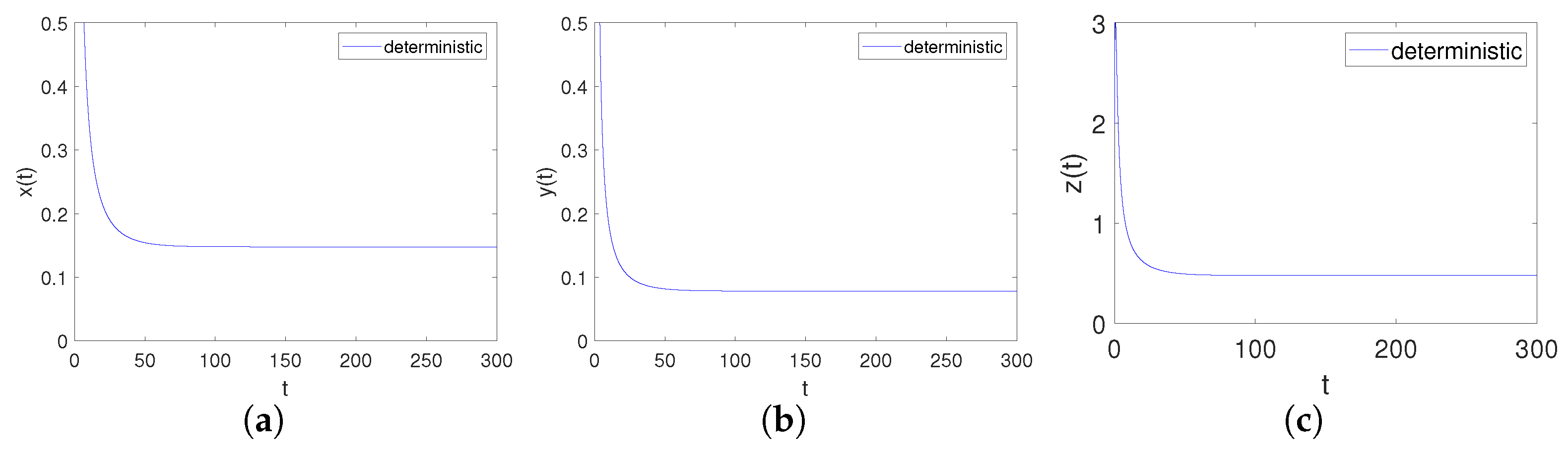
Obviously, the trivial equilibrium point of the system is $E_0:(0,0,0)$. It can be obtained by Matlab version $\mathtt{R}\mathtt{2023}\mathtt{b}$ that the eigenvalues of its corresponding Jacobian matrix are ${\lambda }_1=-0.01$, ${\lambda }_2=-0.0367$, ${\lambda }_3=-1.3633$, $R_0=0.8889$. Apparently, ${\lambda }_1,{\lambda }_2,{\lambda }_3<0$, $R_0<1$, namely $E_0:(0,0,0)$ is locally asymptotical. This is consistent with point 1 of Theorem 3, as shown in Figure 2.

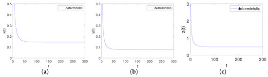
Figure 2. Time-series diagrams of each population for deterministic system (4) satisfying Case I. (a) Time-series diagram of $x\left(t\right)$; (b) Time-series diagram of $y\left(t\right)$; (c) Time-series diagram of $z\left(t\right)$.

(2)

When Case II is satisfied, deterministic system (4) takes the following form

$$\left\{\begin{array}{c}{\displaystyle \frac{\mathrm{d}x\left(t\right)}{\mathrm{d}t}=0.83y-0.8x-0.02x^2-0.01x,}\hfill \\ {\displaystyle \frac{\mathrm{d}y\left(t\right)}{\mathrm{d}t}=0.8x-0.01y^2-0.01y-\frac{0.21yz}{1+0.21y},}\hfill \\ {\displaystyle \frac{\mathrm{d}z\left(t\right)}{\mathrm{d}t}=z\left(\frac{0.063y}{1+0.21y}-\frac{0.6z}{1+y}\right)-0.1z.}\hfill \end{array}\right.$$

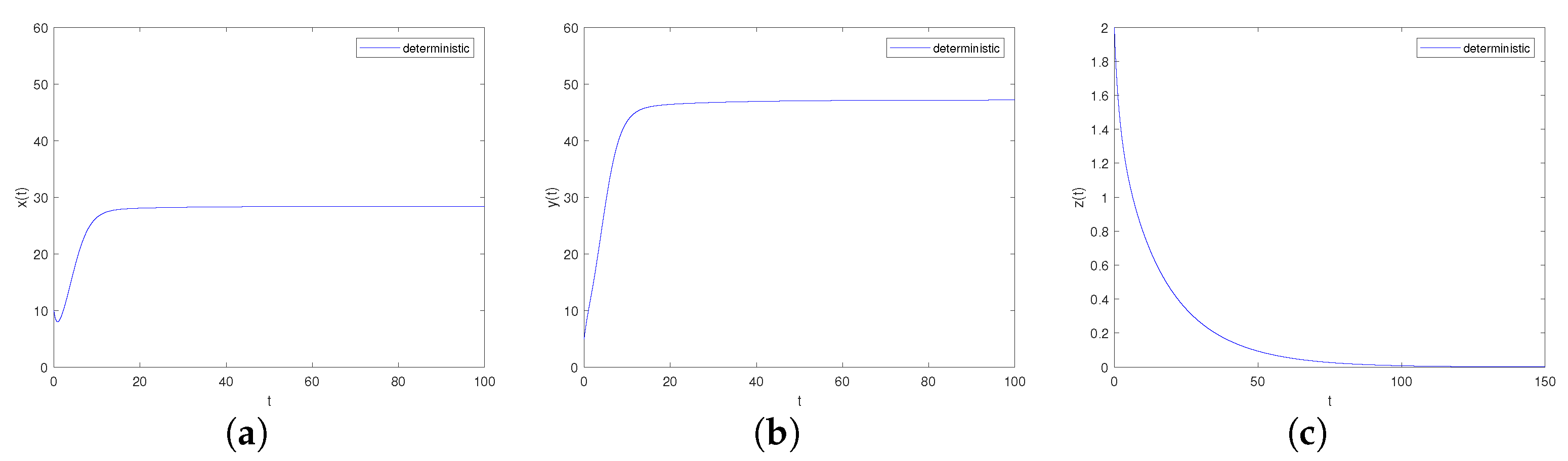
It can be obtained by Matlab version R2023b that the boundary equilibrium point of the system is $\check{E}:(28.41,47.18,0)$ and the eigenvalues of its corresponding Jacobian matrix are ${\lambda }_1=-0.007,$${\lambda }_2=-0.5634,{\lambda }_3=-2.4266$. Obviously, ${\lambda }_1,{\lambda }_2,{\lambda }_3<0$ hold. Further, we can calculate that $R_0=8.1975$, $r_{1}g=0.664$, $(2b\check{x}+g+d_1)(d_2+2f\check{y})=1.6574$, ${\displaystyle \frac{c\beta (1-v)\check{y}}{1+k(1-\nu )\check{y}}}=0.003$, there is, $R_0>1$, $r_{1}g<(2b\check{x}+g+d_1)(d_2+2f\check{y})$, $d_3>{\displaystyle \frac{c\beta (1-v)\check{y}}{1+k(1-\nu )\check{y}}}$, namely the conditons of Theorem 3 point 2 are satisfied. The boundary equilibrium point is asymptotically stable, as shown in Figure 3.

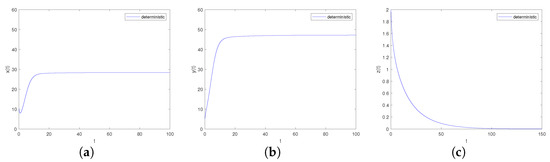
Figure 3. Time-series diagrams of each population for deterministic system (4) satisfying Case II. (a) Time-series diagram of $x\left(t\right)$; (b) Time-series diagram of $y\left(t\right)$; (c) Time-series diagram of $z\left(t\right)$.

(3)

When Case III is satisfied, deterministic system (4) takes the following form

$$\left\{\begin{array}{c}{\displaystyle \frac{\mathrm{d}x\left(t\right)}{\mathrm{d}t}=0.98y-0.45x-0.4x^2-0.01x,}\hfill \\ {\displaystyle \frac{\mathrm{d}y\left(t\right)}{\mathrm{d}t}=0.45x-0.01y^2-0.75y-\frac{0.21yz}{1+0.21y},}\hfill \\ {\displaystyle \frac{\mathrm{d}z\left(t\right)}{\mathrm{d}t}=z\left(\frac{0.063y}{1+0.21y}-\frac{0.3z}{1+y}\right)-0.01z.}\hfill \end{array}\right.$$

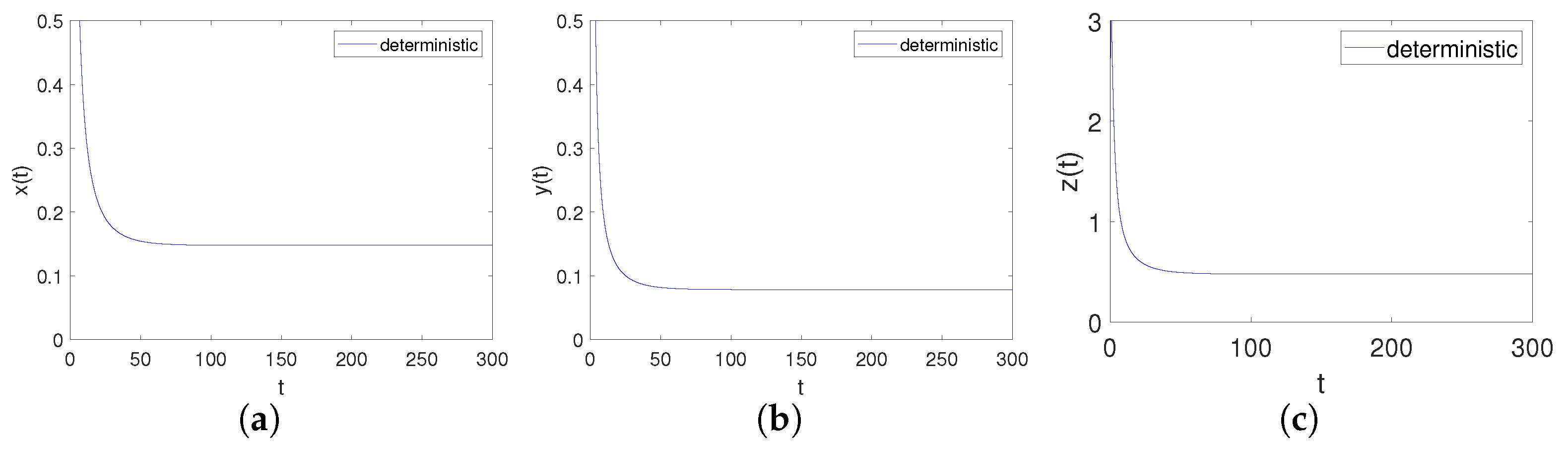
It can be obtained by Matlab version R2023b that the positive equilibrium point of the system is $E^{*}:(0.15,0.08,0.48)$ and the eigenvalues of its corresponding Jacobian matrix are ${\lambda }_1=-0.0374,{\lambda }_2=-0.2743,{\lambda }_3=-1.3906$. Obviously, ${\lambda }_1,{\lambda }_2,{\lambda }_3<0$ hold. Further, we can calculate that $R_0=1.2783$, $\xi =0.1427$, $\check{x}=0.5018$, $A_1+A_2+A_3=1.2599$, $A_1{A}_2{A}_3+A_{1}B-A_3{r}_{1}g=0.021$, $(A_1{A}_2-r_{1}g)(A_1+A_2)+A_1{A}_3(A_1+A_3)+(A_2{A}_3+B)(A_2+A_3)+2A_1{A}_2{A}_3=1.062$. Apparently, $R_0>1$, $0<\xi <\check{x}$ and $\left[Q_1\right]$, $\left[Q_2\right]$, $\left[Q_3\right]$ hold, namely $E^{*}:(x^{*},y^{*},z^{*})$ is locally asymptotical. This corresponds to point 3 of Theorem 3, as shown in Figure 4.

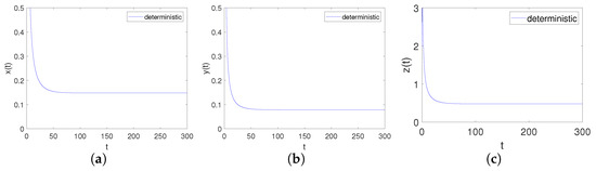
Figure 4. Time-series diagrams of each population for deterministic system (4) satisfying Case III. (a) Time-series diagram of $x\left(t\right)$; (b) Time-series diagram of $y\left(t\right)$; (c) Time-series diagram of $z\left(t\right)$.

4.2. Numerical Simulations of Stochastic System (6)

Next, the numerical simulation of stochastic system (6) is shown. From Milstein’s Higher-Order method [36], the following discrete system corresponding to system (6) is obtained

$$\left\{\begin{array}{c}{\displaystyle x_{n+1}=x_n+(r_1{y}_n-b{x}_n^2-g{x}_n-d_1{x}_n)\Delta t+{\sigma }_1{x}_n{\zeta }_{1,n}\sqrt{\Delta t}+\frac{{\sigma }_1^2}{2}{x}_n({\zeta }_{1,n}^2-1)\Delta t,}\hfill \\ {\displaystyle y_{n+1}=y_n+\left(g{x}_n-d_2{y}_n-\frac{\beta (1-\nu )y_n{z}_n}{1+k(1-\nu )y_n}-f{y}_n^2\right)\Delta t+{\sigma }_2{y}_n{\zeta }_{2,n}\sqrt{\Delta t}+\frac{{\sigma }_2^2}{2}{y}_n({\zeta }_{2,n}^2-1)\Delta t,}\hfill \\ {\displaystyle z_{n+1}=z_n+\left(-\frac{r_2{z}_n^2}{h+y_n}+\frac{c\beta (1-\nu )y_n{z}_n}{1+k(1-\nu )y_n}-d_3{z}_n\right)\Delta t+{\sigma }_3{z}_n{\zeta }_{3,n}\sqrt{\Delta t}+\frac{{\sigma }_3^2}{2}{z}_n({\zeta }_{3,n}^2-1)\Delta t,}\hfill \end{array}\right.$$

(35)

where $\Delta t=0.01$, ${\zeta }_{i,n},i=1,2,3$ are the Gaussian random variables, which obey the Gaussian distribution $N(0,1)$.

(1)

Let ${\sigma }_1=1.3$, ${\sigma }_2=1.3$, ${\sigma }_3=1.5$; if the other parameters are the same as in Case I, we can derive $\rho =-0.075<0$. From Theorem 9, we know that both the prey and predator become extinct (see Figure 5a–c). Comparing Figure 5 and Figure 6, with the increase in environmental noise intensity, the prey population will go from persistent to extinct.

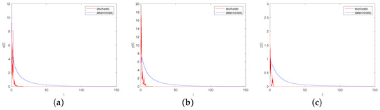Figure 5. Time-series diagrams of each population for stochastic system (6) with ${\sigma }_1={\sigma }_2=1.3$, ${\sigma }_3=1.5$. (a) Time-series diagram of $x\left(t\right)$; (b) Time-series diagram of $y\left(t\right)$; (c) Time-series diagram of $z\left(t\right)$.

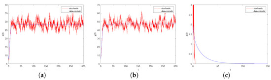Figure 6. Time-series diagrams of each population for stochastic system (6) with ${\sigma }_1={\sigma }_2=0.1$, ${\sigma }_3=1.5$. (a) Time-series diagram of $x\left(t\right)$; (b) Time-series diagram of $y\left(t\right)$; (c) Time-series diagram of $z\left(t\right)$.

(2)

Let ${\sigma }_1=0.1$, ${\sigma }_2=0.1$, ${\sigma }_3=1.5$; if the other parameters are the same as in Case II, it is verified that ${\lambda }_0={\displaystyle \frac{c\beta }{k}}-d_3-{\displaystyle \frac{{\sigma }_3^2}{2}}=-1.095<0$ and $R^{*}=1.01>1$, which meet the criteria of Theorem 8, i.e., the scenario depicted in Figure 6a–c: the predator population $z\left(t\right)$ will die out while the prey populations $x\left(t\right)$ and $y\left(t\right)$ will persist.

(3)

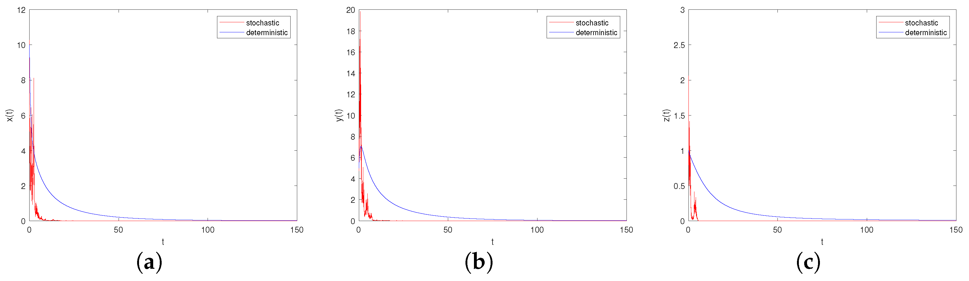
Let ${\sigma }_1=0.1$, ${\sigma }_2=0.1$, ${\sigma }_3=0.1$; if the other parameters are the same as in Case III, we can easily check that $R_0^s=1.0001>1$, $d=min\left\{d_1,d_2,d_3\right\}=0.01>0.005={\displaystyle \frac{1}{2}}max\left\{{\sigma }_1^2,{\sigma }_2^2,{\sigma }_3^2\right\}$. Through Theorem 10, we can conclude that system (6) provides a unique ergodic stationary distribution. As shown in Figure 7a–c, when the environmental noises are sufficiently small, it will not have a significant impact on the persistence of system (6).

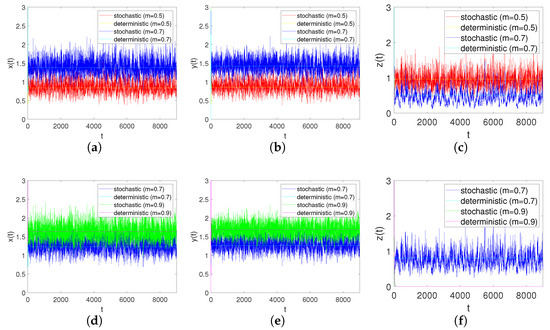
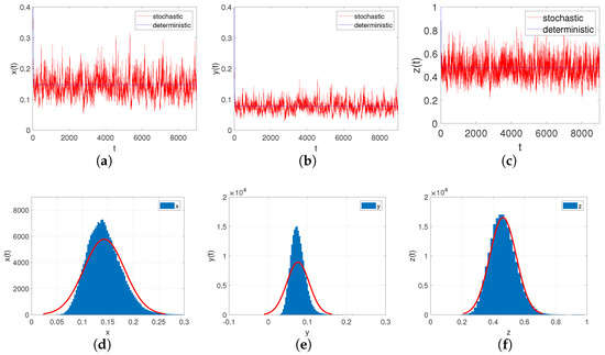Figure 7. (a–c): Time-series diagrams of each population for stochastic system (6) with ${\sigma }_1={\sigma }_2={\sigma }_3=0.1$; (d–f): The histograms and marginal density functions of solution.

In order to adequately demonstrate the effects of the modified Leslie–Gower for system responses, we consider the two cases $h=1$ and $h=10$ while keeping all of the other coefficients unchanged. From Figure 8a–c, we can analyse that when h increases, i.e., the predator’s survival environment is improved, it causes the number of prey populations to decrese and, at the same time, it makes the number of predator populations increase.

Figure 8. Time-series diagrams of the stochastic system (6) and its corresponding deterministic system (4) with $h=1$ and $h=10$. (a) Time-series diagram of $x\left(t\right)$; (b) Time-series diagram of $y\left(t\right)$; (c) Time-series diagram of $z\left(t\right)$.

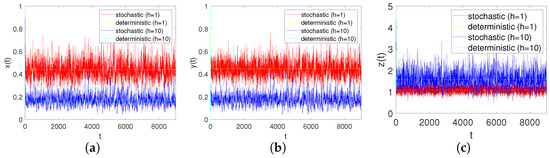
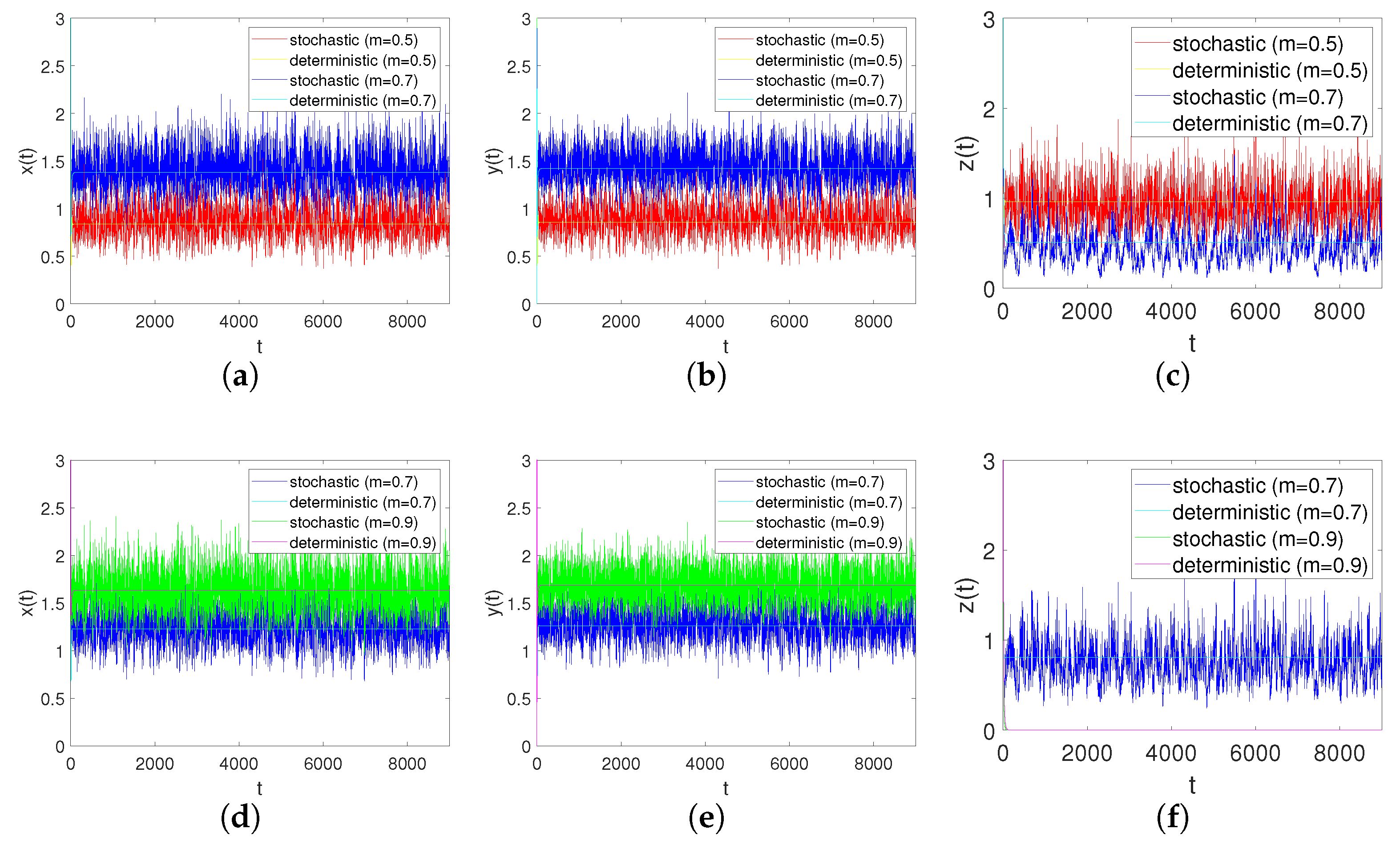
In order to verify the effect of the refuge on the system, we consider the cases $\nu =0.5$, $\nu =0.7$ and $\nu =0.9$, while keeping the other coefficients unchanged. From Figure 9a–c, we can conclude that when $\nu =0.5$ is changed to $\nu =0.7$; that is, when more shelters are provided for prey, the number of prey will increase and the number of predator will decrease. According to Figure 9d–f, when $\nu =0.7$ becomes $\nu =0.9$, that is, when the prey refuge is large enough, the number of prey population will further increase, but it will lead to the extinction of predators.

Figure 9. (a–c): Time series diagrams of stochastic system (6) and its corresponding deterministic system (4) with $\nu =0.5$, $\nu =0.7$; (d–f): Time series diagrams of stochastic system (6) and its corresponding deterministic system (4) with $\nu =0.7$, $\nu =0.9$.

5. Conclusions

In this paper, a predator–prey model with a two-stage structure of a prey population is constructed, in which the environmental capacity of predator is described by the Leslie–Gower modification term, while the prey population has a shelter effect.

For the deterministic model (4), the existence, uniqueness, non-negativity, and uniform boundedness for the solution of the system are discussed first. Then, the threshold condition $R_0={\displaystyle \frac{r_{1}g}{d_2(g+d_1)}}$ for the existence of the equilibrium point is obtained. If $R_0<1$, then $E:(0,0,0)$ exists and is locally asymptotically stable; if $R_0>1$, then, there is a unique boundary equilibrium point $\check{E}:(\check{x},\check{y},0)$; when $R_0>1$, $c\beta <k{d}_3$, and $\xi <\check{x}$ hold, a positive equilibrium point $E^{*}:(x^{*},y^{*},z^{*})$ exist. Further, when $R_0>1$, whether the inequality $c\beta >k{d}_3$ is established becomes another key condition to determine the stability of the equilibrium point $\check{E}$ and $E^{*}$.

For the stochastic model (6), the existence of global positive solutions and stochastic boundedness are discussed at first. Then, the long-term dynamic properties of the system are discussed. If the degree of the white noise ${\sigma }_i^2(i=1,2,3)$ is large enough such that $\rho <0$, the system goes extinct. Conversely, if ${\sigma }_i^2(i=1,2,3)$ are small enough, such that $R_0^s>1$, then there is an ergodic stationary distribution and the system is persistent.

Finally, the deterministic model and the stochastic model are simulated by Matlab version R2023b, and the effects of the predator environment improvement and prey shelter effect on the population dynamics are discussed.

References

- Leslie, P.H. Some further notes on the use of matrices in population mathematics. Biometrika 1948, 35, 213–245. [Google Scholar] [CrossRef]
- Leslie, P.H.; Gower, J.C. The properties of a stochastic model for the predator-prey type of interaction between two species. Biometrika 1960, 47, 219–234. [Google Scholar] [CrossRef]
- Wollkind, D.J.; Collings, J.B.; Logan, J.A. Metastability in a temperature-dependent model system for predator-prey mite outbreak interactions on fruit trees. Bull. Math. Biol. 1988, 50, 379–409. [Google Scholar] [CrossRef]
- Mi, Y.Y.; Song, C.; Wang, Z.C. Global boundedness and dynamics of a diffusive predator-prey model with modified Leslie-Gower functional response and density-dependent motion. Commun. Nonlinear Sci. Numer. Simul. 2023, 119, 107115. [Google Scholar] [CrossRef]
- Chen, M.; Takeuchi, Y.; Zhang, J.F. Dynamic complexity of a modified Leslie-Gower predator-prey system with fear effect. Commun. Nonlinear Sci. Numer. Simul. 2023, 119, 107109. [Google Scholar] [CrossRef]
- Qiu, H.; Guo, S. Bifurcation structures of a Leslie-Gower model with diffusion and advection. Appl. Math. Lett. 2023, 135, 108391. [Google Scholar] [CrossRef]
- Li, Y.; Xiao, D. Bifurcations of a predator-prey system of Holling and Leslie types. Chaos Solitons Fract. 2007, 34, 606–620. [Google Scholar] [CrossRef]
- Nindjin, A.F.; Aziz-Alaoui, M.A.; Cadivel, M. Analysis of a predator-prey model with modified Leslie-Gower and Holling-type II schemes with time delay. Nonlinear Anal. Real World Appl. 2006, 7, 1104–1118. [Google Scholar] [CrossRef]
- Aziz-Alaoui, M.A.; Okiye, M.D. Boundedness and global stability for a predator-prey model with modified Leslie-Gower and Holling-type II schemes. Appl. Math. Lett. 2003, 16, 1069–1075. [Google Scholar] [CrossRef]
- Hanski, I.; Hansson, L.; Henttonen, H. Specialist predators, generalist predators, and the microtine rodent cycle. J. Anim. Ecol. 1991, 60, 353–367. [Google Scholar] [CrossRef]
- Upadhyay, R.K.; Rai, V. Why chaos is rarely observed in natural populations. Chaos Solitons Fract. 1997, 8, 1933–1939. [Google Scholar] [CrossRef]
- Puchuri, L.; González-Olivares, E.; Rojas-Palma, A. Multistability in a Leslie-Gower-type predation model with a rational nonmonotonic functional response and generalist predators. Comput. Math. Method M 2020, 2, e1070. [Google Scholar] [CrossRef]
- Wang, W.; Zhou, M.; Fan, X.; Zhang, T. Global dynamics of a nonlocal PDE model for Lassa haemorrhagic fever transmission with periodic delays. Comput. Appl. Math. 2024, 43, 140. [Google Scholar] [CrossRef]
- Zhang, X.; Chen, L.; Neumann, A.U. The stage-structured predator-prey model and optimal harvesting policy. Math. Biosci. 2000, 168, 201–210. [Google Scholar] [CrossRef] [PubMed]
- Maiti, A.P.; Dubey, B.; Chakraborty, A. Global analysis of a delayed stage structure prey-predator model with Crowley-Martin type functional response. Math. Comput. 2019, 162, 58–84. [Google Scholar] [CrossRef]
- Zhang, S.; Yuan, S.; Zhang, T. A predator-prey model with different response functions to juvenile and adult prey in deterministic and stochastic environments. Appl. Math. Comput. 2022, 413, 126598. [Google Scholar] [CrossRef]
- Wang, R.; Zhao, W. Extinction and stationary distribution of a stochastic predator-prey model with Holling II functional response and stage structure of prey. J. Appl. Anal. Comput. 2022, 12, 50–68. [Google Scholar]
- Xiao, Z.; Li, Z.; Zhu, Z.; Chen, F. Hopf bifurcation and stability in a Beddington-DeAngelis predator-prey model with stage structure for predator and time delay incorporating prey refuge. Open Math. 2019, 17, 141–159. [Google Scholar] [CrossRef]
- Wang, W.; Wang, X.; Fan, X. Threshold dynamics of a reaction-advection-diffusion waterborne disease model with seasonality and human behavior change. Int. J. Biomath. 2024, 2350106. [Google Scholar] [CrossRef]
- McNair, J.N. The effects of refuges on predator-prey interactions: A reconsideration. Theor. Popul. Biol. 1986, 29, 38–63. [Google Scholar] [CrossRef]
- McNair, J.N. Stability effects of prey refuges with entry-exit dynamics. J. Theor. Biol. 1987, 125, 449–464. [Google Scholar] [CrossRef]
- Jamil, A.R.M.; Naji, R.K. Modeling and analysis of the influence of fear on the harvested modified Leslie–Gower model involving nonlinear prey refuge. Mathematics 2022, 10, 2857. [Google Scholar] [CrossRef]
- Xiang, C.; Huang, J.; Wang, H. Bifurcations in Holling-Tanner model with generalist predator and prey refuge. J. Differ. Equ. 2023, 343, 495–529. [Google Scholar] [CrossRef]
- Zhang, H.; Cai, Y.; Fu, S.; Wang, W. Impact of the fear effect in a prey-predator model incorporating a prey refuge. Appl. Math. Comput. 2019, 356, 328–337. [Google Scholar] [CrossRef]
- Verma, M.; Misra, A.K. Modeling the effect of prey refuge on a ratio-dependent predator-prey system with the Allee effect. Bull. Math. Biol. 2018, 80, 626–656. [Google Scholar] [CrossRef] [PubMed]
- Liu, Q.; Jiang, D. Stationary distribution and probability density for a stochastic SEIR-type model of coronavirus (COVID-19) with asymptomatic carriers. Chaos Solitons Fract. 2023, 169, 113256. [Google Scholar] [CrossRef] [PubMed]
- Feng, T.; Zhou, H.; Qiu, Z.; Kang, Y. Impacts of demographic and environmental stochasticity on population dynamics with cooperative effects. Math. Biosci. 2022, 353, 108910. [Google Scholar] [CrossRef] [PubMed]
- Feng, T.; Milne, R.; Wang, H. Variation in environmental stochasticity dramatically affects viability and extinction time in a predator-prey system with high prey group cohesion. Math. Biosci. 2023, 365, 109075. [Google Scholar] [CrossRef] [PubMed]
- Yang, A.; Wang, H.; Yuan, S. Tipping time in a stochastic Leslie predator-prey model. Chaos Solitons Fract. 2023, 171, 113439. [Google Scholar] [CrossRef]
- Venkataiah, K.; Ramesh, K. On the stability of a Caputo fractional order predator-prey framework including Holling type-II functional response along with nonlinear harvesting in predator. Partial Differ. Equ. Appl. Math. 2024, 11, 100777. [Google Scholar]
- Wang, X.A. Simple proof of Descartes’s rule of signs. Am. Math. Mon. 2004, 111, 525–526. [Google Scholar] [CrossRef]
- Al-Azzawi, S.F. Stability and bifurcation of pan chaotic system by using Routh-Hurwitz and Gardan methods. Appl. Math. Comput. 2012, 219, 1144–1152. [Google Scholar] [CrossRef]
- LaSalle, J.P.; Lefschetz, S. Stability by Lyapunov’s Direct Method with Applications; Academic Press: New York, NY, USA, 1961. [Google Scholar]
- Mao, X. Stochastic Differential Equations and Applications; Elsevier: Amsterdam, The Netherlands, 2007. [Google Scholar]
- Li, J.; Liu, X.; Wei, C. The impact of role reversal on the dynamics of predator-prey model with stage structure. Appl. Math. Modell. 2022, 104, 339–357. [Google Scholar] [CrossRef]
- Higham, D.J. An algorithmic introduction to numerical simulation of stochastic differential equations. SIAM Rev. 2001, 43, 525–546. [Google Scholar] [CrossRef]
Disclaimer/Publisher’s Note: The statements, opinions and data contained in all publications are solely those of the individual author(s) and contributor(s) and not of MDPI and/or the editor(s). MDPI and/or the editor(s) disclaim responsibility for any injury to people or property resulting from any ideas, methods, instructions or products referred to in the content. |
© 2024 by the authors. Licensee MDPI, Basel, Switzerland. This article is an open access article distributed under the terms and conditions of the Creative Commons Attribution (CC BY) license (https://creativecommons.org/licenses/by/4.0/).