Fractional Dynamics of Cassava Mosaic Disease Model with Recovery Rate Using New Proposed Numerical Scheme

Abstract

Food security is a basic human right that guarantees humans an adequate amount of nutritious food. However, plant viruses and agricultural pests cause real damage to food sources, leading to negative impacts on meeting the human right of obtaining a sufficient amount of food. Understanding infectious disease dynamics can help us to design appropriate control and prevention strategies. Although cassava is among the most produced and consumed crops and greatly contributes to food security, cassava mosaic disease causes a decrease in photosynthesis and reduces cassava yield, resulting in a lack of crops. This paper developed a fractional model for cassava mosaic disease (CMD) dynamics based on the Caputo–Fabrizio (CF) fractional derivative to decrease cassava plant infection. We used fixed-point theory to study the existence of a unique solution in the form of the CMD model. A stability analysis of the model was conducted by using fixed-point theory and the Picard technique. A new numerical scheme was proposed for solving the nonlinear system of a fractional model in the sense of the CF-derivative and applied to obtain numerical simulations for a fractional model of the dynamics of CMD. The obtained results are described using figures that show the dynamics and behaviors of the compartments of CMD, and it is concluded that decreasing the population of whitefly vectors can prevent cassava plants from becoming infected better than increasing the recovery rate of the infected cassava plants.

1. Introduction

Cassava (Manioc) is an important food crop for most countries that grows in tropical and subtropical regions. It originated in South America and was then brought from Brazil into some countries in West Africa by Portuguese mariners at the beginning of the sixteenth century. Then, its planting area expanded in the eighteenth century into some countries in East Africa and other regions in India, Indonesia, and the Philippines [1]. It can be planted in various environmental conditions and withstand long periods of dryness. Another advantage of its tuberous roots is that they can be kept in the ground for several months until needed for feeding or consumption. Additionally, the cassava plant has the adaptability to grow and yield under poor soil fertility conditions, and its crop has a unique capability to produce harvestable yield fruits even under hostile environmental conditions, where other crops fail [2]. According to the Food and Agricultural Organization of the United Nations (FAOUN), cassava is one of the most essential food sources in developing countries after maize, rice, and wheat. In 2018, its global production reached 278 million metric tons, which is an increase of 240 million metric tons from 2010 [3,4].

Different plant diseases are caused by viruses or insects that infect plants, which decrease crop production and lead to food insecurity problems. Mosaic disease is one of the diseases that cause enormous damage to various global agricultural goods, including tuberous roots, tomatoes, peppers, and aubergines with an estimated loss of between 40 and 70 percent of annual production. Cassava is one of the largest food harvest crops worldwide, and its related manufacturing plays an essential role in the agricultural economy and production safety. However, cassava mosaic disease (CMD) eliminates cassava and Jatropha plants in tropical areas, such as Africa, Asia, and South America. The virus that causes CMD is begomovirus, which is transmitted by Bemisia tabaci whiteflies over short distances in the field in a particular circulation mode and can be transmitted over long distances with the assistance of infected stems [5]. Several optimal control and prevention strategies have been employed for CMD, such as re-plantation (removing sick plants and replacing them with healthy ones) and roguing (removing infected cassava plants). Other strategies applied to disease vectors include treatment with biological techniques and pesticides and creating a new plant with vector-resistant plant properties. However, CMD still causes serious damage in production every year.

Mathematical modeling is a branch of mathematics that is extremely important in representing real-world scenarios in mathematical terms. It helps to make good predictions or provide scientific insights for specific phenomena and simplify them for decision-makers for improvement or further prevention and control purposes. It has recently been used for managing activities that are related to agricultural production, specifically in controlling plant infections and insect pests and establishing prevention and control strategies to prevent or reduce the spread of disease. In [6], the researchers introduced a mathematical model for utilizing plant biomass, pests, and population awareness to explore how people’s awareness impacts crop pest management. The application of integrated pesticides was used to analyze a mathematical model of Jatropha curcas plantation to manage its natural pests [7]. A coffee berry disease spread dynamics model was discussed in [8]. It considers the interaction of fungal pathogens with coffee berry and vector populations. Many studies have used mathematical models to investigate or discuss mosaic disease’s spread dynamics in different kinds of crops. The authors of [9] developed a mathematical model for spore dispersal in order to better understand and predict rice blast disease spreading. In [10], the researchers proposed and analyzed a mathematical model for controlling mosaic disease infections using natural prevention strategies through an RNA interference mechanism to protect the plant from infection and improve plant growth. In [11], the authors introduced a numerical investigation of heavy metal transfer from soil to plants, and they assessed its application to honey contamination. Their study reconstructs proton flow in soil during rainfall and water availability to plant roots over time, aiding in understanding ecosystem vulnerability to metal pollutants, assessing contaminant transfer risks in the food chain, and determining if pollution levels have reached critical ecological thresholds.

Numerous studies have also used mathematical models to study mosaic disease’s transmission effects in plant populations. For example, saturated response functions are used for introducing a mathematical model for studying the dynamics of mosaic disease with farming awareness based on roguing and insect repellent spraying [12]. A delay mathematical model of mosaic disease is introduced to study the dynamics in Jatropha curcas planting with roguing [13]. An epidemiological model is introduced for mosaic disease considering plant compartments and vector populations [14]. In [15], the authors proposed a mathematical model for studying the dynamics of CMD that includes immature and mature vectors, considering the time delay, demonstrating vector maturation time. A Markov chain model with continuous time was used for formulating and analyzing a stochastic epidemic model of the propagation of CMD [16]. In [17], the researchers developed a mathematical model for CMD considering planting using infected cuttings and whitefly transmission.

Currently, fractional calculus techniques provide a better understanding and interpretation of dynamics of the systems and phenomena used to investigate fractal, anomalous, or memory-like behavior. It defines a mathematical framework for describing systems with long-range dependency and non-locality with fractional order dynamics. For example, in [18], the authors used the Caputo fractional derivative for analyzing a diphtheria epidemic model. They concluded that reducing the contact, transmission, and birth rates would be essential strategies for reducing diphtheria transmission. Suganya et al. [19] used a fuzzy fractional Caputo derivative for studying the dynamics of an SIR childhood disease model, indicating that their proposed fractional model is more efficient than the model with an integer order. Fractional calculus has also been used to investigate the dynamics of many complex ecological and biological systems in several fields, including physics and soliton phenomena [20,21], mathematical physics [22], engineering [23], biology [24,25,26], and infectious disease transmission and vaccination [27,28,29,30,31]. For more studies related to the application of fractional calculus in agricultural and food systems, the reader can see [32]. In the case of plant diseases, FDEs have been used to model the spread and dynamics of infections. For example, in [33], the researchers used the Atangana–Baleanu fractional derivative to investigate the dynamics of the plant disease fractional model in preventive and curative stages. The results showed that increasing the roguing rate of the infected plant area or decreasing the planting rate in the infected ones will reduce plant disease transmissions. The viscoelastic behavior of potato tubers was investigated by applying the fractional calculus for their proposed relaxation model [34]. They compared the parameters’ correlation based on the FDEs with a generalized Maxwell model, and they concluded that the fractional model can replace the generalized Maxwell model to achieve the same accuracy with fewer parameters. In [35], the researchers used FDEs to study the transmission dynamics of pests in tea plants. They investigated some control strategies to reduce the effects of biological enemies in the frame.

Regarding the application of fractional calculus in mosaic disease infections, ref. [36] introduced a fractional-order model to study the dynamics of jatropha curcas under mosaic virus infection. It focused on bifurcation control under awareness of farming and implementation delay. They found that the Hopf bifurcation progressively occurs in advance, as the fractional order has a bigger value with extreme points’ existence for the response gain and the extended response delay that can reduce the bifurcation value. In [37], they analyzed two different nonlinear mosaic disease models of plants using the Atangana–Baleanu derivative and Caputo fractional derivative. A fractional model based on the Caputo derivative proposed to investigate the dynamics of CMD [38]. They discussed the existence and stability conditions of the equilibrium points of the model, which concluded that the parameter of the disease transmission rate could result in Hopf bifurcation around the endemic equilibrium. Another study also used the Caputo derivative to study the dynamics of CMD that included the predators population and the impact of seasonality competitions [39]. They observed that the infection almost becomes zero in the case of an integral value, but it always persists as the fractional order is introduced, which is more realistic. To the best of our knowledge, no study investigated the effects of recovery rate on cassava plants with mosaic disease using fractional derivatives.

While these studies introduced better prediction than the classic integer models, adequate results also could not be achieved because of the singularity appearance in the classical fractional derivatives, which made those derivatives insufficient to describe the system dynamics [40]. To move beyond this problem, the Caputo–Fabrizio fractional derivative (CF) [41] with a non-singular kernel was proposed. It is a non-local fractional operator that is able to describe the material heterogeinity and structures with dissimilar scales, which cannot be well discussed by classical local fractional derivatives. To our knowledge, there is no previous study that discussed the dynamics of CMD with a recovery rate based on the CF-fractional derivative and motivated by the above-mentioned discussions. This study aims to use the CF-derivative to study the dynamics of the proposed CMD model with a recovery rate of the infected cassava plant.

In this study, we consider the CMD fractional model with a recovery rate under treatment. Our findings contribute to understanding the CMD dynamics with recovery rate under CF-fractional derivative. Our study also investigated the effects of increasing the treatment rate and decreasing the whitefly population rate in the cassava plant environment. We also proposed a new numerical scheme that can be applied to obtain numerical solutions of fractional nonlinear systems with a CF-derivative, which can enhance the efficiency and accuracy of future research in this field.

The structure of the paper is organized as follows: The model is introduced in Section 2 using a system of nonlinear equations of the CF-fractional derivative. In Section 3, we give some definitions, theories, and lemmas as preliminary concepts that will be needed during the theoretical and numerical analysis of the study. The existence, uniqueness, and stability of the CMD model solution is studied in Section 4. In Section 5, we introduced a new corrector–predictor scheme and used the proposed scheme to provide a numerical simulation of the CMD fractional model.

2. Basic Model Structure

Enhancing the discussions mentioned above, we introduce a fractional model to study the dynamics of CMD in the sense of CF-fractional derivatives. Let $X_C$ be denoted for the healthy cassava plant density (m⁻²), $I_C$ be the infected cassava population (m⁻²), let $X_W$ be the susceptible population of whitefly vectors (m⁻²), and let $I_W$ be the density of the infected whitefly vectors (m⁻²). The maximum plant population is denoted by k (m⁻²), healthy cassava plants are logistically replanting at rate a that is constrained by the maximum plant density (day⁻¹) and can be infected with CMD through the infected whitefly at the rate r (day⁻¹). The model assumes that the harvested rates of the healthy and infected cassava plants are equal and noted by $\psi$ (day⁻¹). The infected cassava can be cured or roguing with the rates $\beta$ and g (day⁻¹), respectively. The whiteflies are logistically growing at the rate b that is assumed to be constrained by the maximum vector abundance (day⁻¹). The rate in which whiteflies vector can get infected from the infected cassava plants is denoted by m (vector⁻¹ day⁻¹). The mortality rate of the infective and non-infective whiteflies both equal and denoted by $\mu$ (day⁻¹).

The following assumptions are constructed according to the dynamics of CMD and were introduced to formulate the CMD model.

• Only healthy cuttings are selected for propagation.
• Diseased cassava plants may be substantially less vigorous than healthy ones, as evidenced by a consistent loss rate due to disease. Any roguing procedures are also considered to increase the loss rate of unhealthy plants.
• The replanting rate for the cassava plant is higher than that for the harvest and roguing rates.
• The propagation rate of whiteflies is higher than the death rate.
• Once a cassava plant gets infected, it remains infectious until recovered or harvested.
• The rate at which the whiteflies vector gets infected from the infected cassava plants and the rate at which the virus acquisition by non-infective vectors is equal.
• Once whiteflies get infected, they remain infectious for life, but their offspring are not infective.

Considering the above-mentioned assumptions, CMD transmission dynamics can be described by the following system of ordinary differential equations

$$\begin{array}{cc}\hfill {\dot{X}}_C\left(t\right)& =a{X}_C\left(t\right)\left(1-{\displaystyle \frac{X_C\left(t\right)+I_C\left(t\right)}{k}}\right)+\beta I_C\left(t\right)-r{I}_W\left(t\right)X_C\left(t\right)-\psi X_C\left(t\right),\hfill \\ \hfill {\dot{I}}_C\left(t\right)& =r{I}_W\left(t\right)X_C\left(t\right)-(\beta +g+\psi )I_C\left(t\right),\hfill \\ \hfill {\dot{X}}_W\left(t\right)& =b\left[X_W\left(t\right)+I_W\left(t\right)\right]\left[1-{\displaystyle \frac{X_W\left(t\right)+I_W\left(t\right)}{\rho +\vartheta \left(X_C\left(t\right)+I_C\left(t\right)\right)}}\right]-m{I}_C\left(t\right)X_W\left(t\right)-\mu X_W\left(t\right),\hfill \\ \hfill {\dot{I}}_W\left(t\right)& =m{I}_C\left(t\right)X_W\left(t\right)-\mu I_W\left(t\right),\hfill \end{array}$$

(1)

subject to the initial conditions

$$X_{C\left(0\right)}\left(t\right)=X_C\left(0\right),I_{C\left(0\right)}\left(t\right)=X_C\left(0\right),X_{W\left(0\right)}\left(t\right)=X_W\left(0\right),I_{W\left(0\right)}\left(t\right)=X_W\left(0\right).$$

(2)

In this study, we analyze alternative representations of the CMD model based on CF-fractional derivatives.

Using System (1), the CMD model with a CF-derivative is given by

$$\begin{array}{cc}\hfill { }_0^{CF}{D}_t^{\eta }{X}_C\left(t\right)& =a{X}_C\left(t\right)\left(1-{\displaystyle \frac{X_C\left(t\right)+I_C\left(t\right)}{k}}\right)+\beta I_C\left(t\right)-r{I}_W\left(t\right)X_C\left(t\right)-\psi X_C\left(t\right),\hfill \\ \hfill { }_0^{CF}{D}_t^{\eta }{I}_C\left(t\right)& =r{I}_W\left(t\right)X_C\left(t\right)-(\beta +g+\psi )I_C\left(t\right),\hfill \\ \hfill { }_0^{CF}{D}_t^{\eta }{X}_W\left(t\right)& =b\left[X_W\left(t\right)+I_W\left(t\right)\right]\left[1-{\displaystyle \frac{X_W\left(t\right)+I_W\left(t\right)}{\rho +\vartheta \left(X_C\left(t\right)+I_C\left(t\right)\right)}}\right]-m{I}_C\left(t\right)X_W\left(t\right)-\mu X_W\left(t\right),\hfill \\ \hfill { }_0^{CF}{D}_t^{\eta }{I}_W\left(t\right)& =m{I}_C\left(t\right)X_W\left(t\right)-\mu I_W\left(t\right),\hfill \end{array}$$

(3)

where ${ }_0^{CF}{D}_t^{\eta }$ represents the $CF$ fractional derivative in the sense of Caputo, and $0<\le 1$ is the fractional order. The model is subject to the initial conditions shown in (2).

3. Fractional Operators

In this section, we investigate some definitions and lemmas that we will use in this work.

Definition 1.

Let $b\ge 0,g\in H^1(0,b)$ and $0<\eta \le 1$; the Caputo fractional derivative of the function g is given by [42]

$${ }_0^C{D}_t^{\eta }\left\{g\left(t\right)\right\}={\displaystyle \frac{1}{\mathsf{\Gamma }(1-\eta )}}{\int }_0^t{(t-\xi )}^{-\eta }{g}^{\prime }\left(\xi \right)d\xi .$$

(4)

To overcome the singularity for $t=\xi$, Caputo and Fabrizio proposed a non-local fractional derivative [41] by replacing the kernel $exp\left[-{\displaystyle \frac{\eta }{1-\eta }}(t-\xi )\right]$ instead of ${(t-\xi )}^{-\eta }$ and ${\displaystyle \frac{\mathbb{T}\left(\eta \right)}{1-\eta }}$ instead of ${\displaystyle \frac{1}{\mathsf{\Gamma }(1-\eta )}}$, where $\mathbb{T}\left(\eta \right)$ is the normalization function that hold the condition $\mathbb{T}\left(0\right)=\mathbb{T}\left(1\right)=1$.

Definition 2.

The Caputo–Fabrizio (CF) fractional derivative in the sense of Liouville–Caputo is given by

$${ }_0^{CF}{D}_t^{\eta }\left\{g\left(t\right)\right\}={\displaystyle \frac{\mathbb{T}\left(\eta \right)}{1-\eta }}{\int }_0^t{g}^{\prime }\left(\xi \right)exp\left[-{\displaystyle \frac{\eta }{1-\eta }}(t-\xi )\right]d\xi ,0<\eta \le 1.$$

(5)

Losada and Nieto [43] studied the properties of CF-derivative and modified it by introducing an exact mathematical expression for the normalization function $\mathbb{T}\left(\eta \right)={\displaystyle \frac{2}{2-\eta }},0<\eta \le 1.$ They introduced the CF-derivative in the following form

$${ }_0^{CF}{D}_t^{\eta }\left\{g\left(t\right)\right\}={\displaystyle \frac{(2-\eta )\mathbb{T}\left(\eta \right)}{2(1-\eta )}}{\int }_0^t{g}^{\prime }\left(\xi \right)exp\left[-{\displaystyle \frac{\eta }{1-\eta }}(t-\xi )\right]d\xi ,0<\eta \le 1,$$

(6)

where

$$\mathbb{T}\left(\eta \right)={\displaystyle \frac{2}{2-\eta }},0<\eta \le 1.$$

Definition 3.

The CF fractional integral of order $\eta ,0<\eta \le 1$ of the function $g\left(t\right)$ is defined as [43]

$${ }_0^{CF}{I}_t^{\eta }\left\{g\left(t\right)\right\}={\displaystyle \frac{2(1-\eta )}{(2-\eta )\mathbb{T}\left(\eta \right)}}g\left(t\right)+{\displaystyle \frac{2\eta }{(2-\eta )\mathbb{T}\left(\eta \right)}}{\int }_0^{t}g\left(\xi \right)d\xi ,t\ge 0.$$

(7)

Definition 4.

The Sumudu transform ($\mathcal{ST}$) of the CF-derivative is given by

$$\mathcal{ST}{\{}_0^{CF}{D}_t^{\eta }g\left(t\right)\}\left(s\right)=\mathbb{T}\left(\eta \right){\displaystyle \frac{\mathcal{ST}\left[G\right(s\left)\right]-g\left(0\right)}{1+(s-1)}}.$$

(8)

Theorem 1.

Let $\mathcal{H}$ be a self-map of $\mathcal{B}$ where $(\mathcal{B},\parallel .\parallel )$ is a Banach space. Then, $\mathcal{H}$ is $\mathcal{H}$-stable if for all $d,e\in \mathcal{B}$, the following inequality holds [44,45]

$$\parallel {\mathcal{H}}_d-{\mathcal{H}}_e\parallel \le Q\parallel d-{\mathcal{H}}_d\parallel +q\parallel d-e\parallel ,$$

(9)

where $Q\ge 0$, and $0\le q\le 1$.

4. CMD Model with Caputo–Fabrizio Derivative

4.1. Existence and Uniqueness of CMD Model

Here, we use the fixed-point theorem to define the existence of the solution of System (3). First, we transform System (3) into an integral equation as following

$$\begin{array}{cc}\hfill X_C\left(t\right)-X_C\left(0\right)& {=}_0^{CF}{I}_t^{\eta }\left[a{X}_C\left(t\right)\left(1-{\displaystyle \frac{X_C\left(t\right)+I_C\left(t\right)}{k}}\right)+\beta I_C\left(t\right)-r{I}_W\left(t\right)X_C\left(t\right)-\psi X_C\left(t\right)\right],\hfill \\ \hfill I_C\left(t\right)-I_C\left(0\right)& {=}_0^{CF}{I}_t^{\eta }\left[r{I}_W\left(t\right)X_C\left(t\right)-(\beta +g+\psi )I_C\left(t\right)\right],\hfill \\ \hfill X_W\left(t\right)-X_W\left(0\right)& {=}_0^{CF}{I}_t^{\eta }[b\left[X_W\left(t\right)+I_W\left(t\right)\right]\left[1-{\displaystyle \frac{X_W\left(t\right)+I_W\left(t\right)}{\rho +\vartheta \left(X_C\left(t\right)+I_C\left(t\right)\right)}}\right]\hfill \\ & -m{I}_C\left(t\right)X_W\left(t\right)-\mu X_W\left(t\right)],\hfill \\ \hfill I_W\left(t\right)-I_W\left(0\right)& {=}_0^{CF}{I}_t^{\eta }\left[m{I}_C\left(t\right)X_W\left(t\right)-\mu I_W\left(t\right)\right].\hfill \end{array}$$

(10)

For computational simplifications, we define the following kernels

$$\begin{array}{cc}\hfill & {\mathsf{\Psi }}_1(t,X_C\left(t\right))=a{X}_C\left(t\right)\left(1-{\displaystyle \frac{X_C\left(t\right)+I_C\left(t\right)}{k}}\right)+\beta I_C\left(t\right)-r{I}_W\left(t\right)X_C\left(t\right)-\psi X_C\left(t\right),\hfill \\ \hfill & {\mathsf{\Psi }}_2(t,I_C\left(t\right))=r{I}_W\left(t\right)X_C\left(t\right)-(\beta +g+\psi )I_C\left(t\right),\hfill \\ \hfill & {\mathsf{\Psi }}_3(t,X_W\left(t\right))=b\left[X_W\left(t\right)+I_W\left(t\right)\right]\left[1-{\displaystyle \frac{X_W\left(t\right)+I_W\left(t\right)}{\rho +\vartheta \left(X_C\left(t\right)+I_C\left(t\right)\right)}}\right]-m{I}_C\left(t\right)X_W\left(t\right)-\mu X_W\left(t\right)\hfill \\ \hfill & {\mathsf{\Psi }}_4(t,I_W\left(t\right))=m{I}_C\left(t\right)X_W\left(t\right)-\mu I_W\left(t\right).\hfill \end{array}$$

(11)

Using the fractional integral of order η given by Equation (7), we obtain

$$\begin{array}{cc}\hfill X_C\left(t\right)=& X_C\left(0\right)+{\displaystyle \frac{2(1-\eta )}{(2-\eta )\mathbb{T}\left(\eta \right)}}{\mathsf{\Psi }}_1(t,X_C\left(t\right))+{\displaystyle \frac{2\eta }{(2-\eta )\mathbb{T}\left(\eta \right)}}{\int }_0^t{\mathsf{\Psi }}_1(\xi ,X_C\left(\xi \right))d\xi ,\hfill \\ \hfill I_C\left(t\right)=& I_C\left(0\right)+{\displaystyle \frac{2(1-\eta )}{(2-\eta )\mathbb{T}\left(\eta \right)}}{\mathsf{\Psi }}_2(t,I_C\left(t\right))+{\displaystyle \frac{2\eta }{(2-\eta )\mathbb{T}\left(\eta \right)}}{\int }_0^t{\mathsf{\Psi }}_2(\xi ,I_C\left(\xi \right))d\xi ,\hfill \\ \hfill X_W\left(t\right)=& X_W\left(0\right)+{\displaystyle \frac{2(1-\eta )}{(2-\eta )\mathbb{T}\left(\eta \right)}}{\mathsf{\Psi }}_3(t,X_W\left(t\right))+{\displaystyle \frac{2\eta }{(2-\eta )\mathbb{T}\left(\eta \right)}}{\int }_0^t{\mathsf{\Psi }}_3(\xi ,X_W\left(\xi \right))d\xi ,\hfill \\ \hfill I_W\left(t\right)=& I_W\left(0\right)+{\displaystyle \frac{2(1-\eta )}{(2-\eta )\mathbb{T}\left(\eta \right)}}{\mathsf{\Psi }}_4(t,I_W\left(t\right))+{\displaystyle \frac{2\eta }{(2-\eta )\mathbb{T}\left(\eta \right)}}{\int }_0^t{\mathsf{\Psi }}_4(\xi ,I_W\left(\xi \right))d\xi .\hfill \end{array}$$

(12)

Theorem 2.

The kernels ${\mathsf{\Psi }}_1,{\mathsf{\Psi }}_2,{\mathsf{\Psi }}_3,$ and ${\mathsf{\Psi }}_4$ satisfy the Lipschitz condition.

Proof. 

We prove that each proposed kernel satisfies the Lipschitz condition. Let $X_C$ and $X_C^{*}$ for the kernel ${\mathsf{\Psi }}_1$, $I_C$ and $I_C^{*}$ for the kernel ${\mathsf{\Psi }}_2$, $X_W$ and $X_W^{*}$ for the kernel ${\mathsf{\Psi }}_3$, and $I_W$ and $I_W^{*}$ for the kernel ${\mathsf{\Psi }}_4$; then, we obtain the following

$$\begin{array}{cc}\hfill \parallel {\mathsf{\Psi }}_1(t,X_C\left(t\right))-{\mathsf{\Psi }}_1(t,X_C^{*}\left(t\right))\parallel =& \parallel a{X}_C\left(t\right)\left(1-{\displaystyle \frac{X_C\left(t\right)+I_C\left(t\right)}{k}}\right)+\beta I_C\left(t\right)-r{I}_W\left(t\right)X_C\left(t\right)\hfill \\ & -\psi X_C\left(t\right)-a{X}_C^{*}\left(t\right)\left(1-{\displaystyle \frac{X_C^{*}\left(t\right)+I_C\left(t\right)}{k}}\right)-\beta I_C\left(t\right)\hfill \\ & +r{I}_W\left(t\right)X_C^{*}\left(t\right)+\psi X_C^{*}\left(t\right)\parallel ,\hfill \\ \hfill \parallel {\mathsf{\Psi }}_2(t,I_C\left(t\right))-{\mathsf{\Psi }}_2(t,I_C^{*}\left(t\right))\parallel =& \parallel r{I}_W\left(t\right)X_C\left(t\right)-(\beta +g+\psi )I_C\left(t\right)-r{I}_W\left(t\right)X_C\left(t\right)\hfill \\ & +(\beta +g+\psi )I_C^{*}\left(t\right)\parallel ,\hfill \\ \hfill \parallel {\mathsf{\Psi }}_3(t,X_W\left(t\right))-{\mathsf{\Psi }}_3(t,X_W^{*}\left(t\right))\parallel =& \parallel b\left[X_W\left(t\right)+I_W\left(t\right)\right]\left[1-{\displaystyle \frac{X_W\left(t\right)+I_W\left(t\right)}{\rho +\vartheta \left(X_C\left(t\right)+I_C\left(t\right)\right)}}\right]\hfill \\ & -m{I}_C\left(t\right)X_W\left(t\right)-\mu X_W\left(t\right)-b\left[X_W^{*}\left(t\right)+I_W\left(t\right)\right][1\hfill \\ & -{\displaystyle \frac{X_W^{*}\left(t\right)+I_W\left(t\right)}{\rho +\vartheta \left(X_C\left(t\right)+I_C\left(t\right)\right)}}]+m{I}_C\left(t\right)X_W^{*}\left(t\right)+\mu X_W^{*}\left(t\right)\parallel ,\hfill \\ \hfill \parallel {\mathsf{\Psi }}_4(t,I_W\left(t\right))-{\mathsf{\Psi }}_4(t,I_W^{*}\left(t\right))\parallel =& \parallel m{I}_C\left(t\right)X_W\left(t\right)-\mu I_W\left(t\right)-m{I}_C\left(t\right)X_W\left(t\right)+\mu I_W^{*}\left(t\right)\parallel .\hfill \end{array}$$

(13)

Using Cauchy’s inequality in Equation (13) and doing some mathematical calculations, we obtain

$$\begin{array}{cc}\hfill \parallel {\mathsf{\Psi }}_1(t,X_C\left(t\right))-{\mathsf{\Psi }}_1(t,X_C^{*}\left(t\right))\parallel \le & \left[a+{\displaystyle \frac{a\parallel X_C\left(t\right)\parallel }{k}}+{\displaystyle \frac{a\parallel X_C^{*}\left(t\right)\parallel }{k}}+{\displaystyle \frac{a\parallel I_C\left(t\right)\parallel }{k}}+r\parallel I_W\left(t\right)\parallel +\psi \right]\hfill \\ & \times \parallel X_C\left(t\right)-X_C^{*}\left(t\right)\parallel ,\hfill \\ \hfill \parallel {\mathsf{\Psi }}_2(t,I_C\left(t\right))-{\mathsf{\Psi }}_2(t,I_C^{*}\left(t\right))\parallel \le & (\beta +g+\psi )\parallel I_C\left(t\right)-I_C^{*}\left(t\right)\parallel ,\hfill \\ \hfill \parallel {\mathsf{\Psi }}_3(t,X_W\left(t\right))-{\mathsf{\Psi }}_3(t,X_W^{*}\left(t\right))\parallel \le & [b+\mu +m\parallel I_C\left(t\right)\parallel +{\displaystyle \frac{2b\parallel I_W\left(t\right)\parallel }{\rho +\vartheta \left(\parallel X_C\left(t\right)\parallel +\parallel I_C\left(t\right)\parallel \right)}}\hfill \\ & +{\displaystyle \frac{b\left(\parallel X_W\left(t\right)\parallel +\parallel X_W^{*}\left(t\right)\parallel \right)}{\rho +\vartheta \left(\parallel X_C\left(t\right)\parallel +\parallel I_C\left(t\right)\parallel \right)}}]\times \parallel X_W\left(t\right)-X_W^{*}\left(t\right)\parallel ,\hfill \end{array}$$

$$\parallel {\mathsf{\Psi }}_4(t,I_W\left(t\right))-{\mathsf{\Psi }}_4(t,I_W^{*}\left(t\right))\parallel \le \mu \parallel I_W\left(t\right))-\mu I_W^{*}\left(t\right)\parallel .$$

(14)

Let $l_1,l_2,l_3,l_4,l_5,$ and $l_6$ be upper bounds of the functions $X_C\left(t\right),X_C^{*}\left(t\right),I_C\left(t\right),X_W\left(t\right),$$X_W^{*}\left(t\right),$ and $I_W\left(t\right)$, respectively; i.e., $\parallel X_C\left(t\right)\parallel \le l_1$, $\parallel X_C^{*}\left(t\right)\parallel \le l_2$, $\parallel I_C\left(t\right)\parallel \le l_3$, $\parallel X_W\left(t\right)\parallel \le l_4$, $\parallel X_W^{*}\left(t\right)\parallel \le l_5$, and $\parallel I_W\left(t\right)\parallel \le l_6$, we obtain

$$\begin{array}{cc}\hfill \parallel {\mathsf{\Psi }}_1(t,X_C\left(t\right))-{\mathsf{\Psi }}_1(t,X_C^{*}\left(t\right))\parallel \le & {\alpha }_1\parallel X_C\left(t\right)-X_C^{*}\left(t\right)\parallel ,\hfill \\ \hfill \parallel {\mathsf{\Psi }}_2(t,I_C\left(t\right))-{\mathsf{\Psi }}_2(t,I_C^{*}\left(t\right))\parallel \le & {\alpha }_2\parallel I_C\left(t\right)-I_C^{*}\left(t\right)\parallel ,\hfill \\ \hfill \parallel {\mathsf{\Psi }}_3(t,X_W\left(t\right))-{\mathsf{\Psi }}_3(t,X_W^{*}\left(t\right))\parallel \le & {\alpha }_3\parallel X_W\left(t\right)-X_W^{*}\left(t\right)\parallel ,\hfill \\ \hfill \parallel {\mathsf{\Psi }}_4(t,I_W\left(t\right))-{\mathsf{\Psi }}_4(t,I_W^{*}\left(t\right))\parallel \le & {\alpha }_4\parallel I_W\left(t\right))-\mu I_W^{*}\left(t\right)\parallel ,\hfill \end{array}$$

(15)

where

$$\begin{array}{cc}\hfill {\alpha }_1=& a+a{\displaystyle \frac{l_1}{k}}+a{\displaystyle \frac{l_2}{k}}+a{\displaystyle \frac{l_3}{k}}+r{l}_6+\psi ,\hfill \\ \hfill {\alpha }_2=& \beta +g+\psi ,\hfill \\ \hfill {\alpha }_3=& b+\mu +m{l}_3+2b{\displaystyle \frac{l_6}{\rho +\vartheta \left(l_1+l_3\right)}}+b{\displaystyle \frac{l_4}{\rho +\vartheta \left(l_1+l_3\right)}}+b{\displaystyle \frac{l_5}{\rho +\vartheta \left(l_1+l_3\right)}},\hfill \\ \hfill {\alpha }_4=& \mu .\hfill \end{array}$$

(16)

Since all of ${\mathsf{\Psi }}_1,{\mathsf{\Psi }}_2,{\mathsf{\Psi }}_3,$ and ${\mathsf{\Psi }}_4$ have upper bounds, ${\mathsf{\Psi }}_1,{\mathsf{\Psi }}_2,{\mathsf{\Psi }}_3,$ and ${\mathsf{\Psi }}_4$ satisfy the Lipschitz condition where ${\alpha }_1,{\alpha }_2,{\alpha }_3,$ and ${\alpha }_4$ are the corresponding Lipschitz constants, which completes the proof. □

For proving the existence of the solution of System (3), we consider the following recursive formula

$$\begin{array}{cc}\hfill X_{C\left(n\right)}\left(t\right)=& {\displaystyle \frac{2(1-\eta )}{(2-\eta )\mathbb{T}\left(\eta \right)}}{\mathsf{\Psi }}_1(t,X_{C(n-1)}\left(t\right))+{\displaystyle \frac{2\eta }{(2-\eta )\mathbb{T}\left(\eta \right)}}{\int }_0^t{\mathsf{\Psi }}_1(\xi ,X_{C(n-1)}\left(\xi \right))d\xi ,\hfill \\ \hfill I_{C\left(n\right)}\left(t\right)=& {\displaystyle \frac{2(1-\eta )}{(2-\eta )\mathbb{T}\left(\eta \right)}}{\mathsf{\Psi }}_2(t,I_{C(n-1)}\left(t\right))+{\displaystyle \frac{2\eta }{(2-\eta )\mathbb{T}\left(\eta \right)}}{\int }_0^t{\mathsf{\Psi }}_2(\xi ,I_{C(n-1)}\left(\xi \right))d\xi ,\hfill \\ \hfill X_{W\left(n\right)}\left(t\right)=& {\displaystyle \frac{2(1-\eta )}{(2-\eta )\mathbb{T}\left(\eta \right)}}{\mathsf{\Psi }}_3(t,X_{W(n-1)}\left(t\right))+{\displaystyle \frac{2\eta }{(2-\eta )\mathbb{T}\left(\eta \right)}}{\int }_0^t{\mathsf{\Psi }}_3(\xi ,X_{W(n-1)}\left(\xi \right))d\xi ,\hfill \\ \hfill I_{W\left(n\right)}\left(t\right)=& {\displaystyle \frac{2(1-\eta )}{(2-\eta )\mathbb{T}\left(\eta \right)}}{\mathsf{\Psi }}_4(t,I_{W(n-1)}\left(t\right))+{\displaystyle \frac{2\eta }{(2-\eta )\mathbb{T}\left(\eta \right)}}{\int }_0^t{\mathsf{\Psi }}_4(\xi ,I_{W(n-1)}\left(\xi \right))d\xi .\hfill \end{array}$$

(17)

Then, we present the difference between the successive terms and apply norm and triangular inequality properties as following

$$\begin{array}{cc}\hfill {\mathsf{{\rm Y}}}_n\left(t\right)=& \parallel X_{C\left(n\right)}\left(t\right)-X_{C(n-1)}\left(t\right)\parallel \le {\displaystyle \frac{2(1-\eta )}{(2-\eta )\mathbb{T}\left(\eta \right)}}\parallel {\mathsf{\Psi }}_1(t,X_{C(n-1)}\left(t\right))-{\mathsf{\Psi }}_1(t,X_{C(n-2)}\left(t\right))\parallel \hfill \\ & +{\displaystyle \frac{2\eta }{(2-\eta )\mathbb{T}\left(\eta \right)}}\parallel {\int }_0^t\left[{\mathsf{\Psi }}_1(\xi ,X_{C(n-1)}\left(\xi \right))-{\mathsf{\Psi }}_1(\xi ,X_{C(n-2)}\left(\xi \right))\right]\parallel d\xi ,\hfill \\ \hfill {\mathsf{\Phi }}_n\left(t\right)=& \parallel I_{C\left(n\right)}\left(t\right)-I_{C(n-1)}\left(t\right)\parallel \le {\displaystyle \frac{2(1-\eta )}{(2-\eta )\mathbb{T}\left(\eta \right)}}\parallel {\mathsf{\Psi }}_2(t,I_{C(n-1)}\left(t\right))-{\mathsf{\Psi }}_2(t,I_{C(n-2)}\left(t\right))\parallel \hfill \\ & +{\displaystyle \frac{2\eta }{(2-\eta )\mathbb{T}\left(\eta \right)}}\parallel {\int }_0^t\left[{\mathsf{\Psi }}_2(\xi ,I_{C(n-1)}\left(\xi \right))-{\mathsf{\Psi }}_2(\xi ,I_{C(n-2)}\left(\xi \right))\right]\parallel d\xi ,\hfill \\ \hfill {\tau }_n\left(t\right)=& \parallel X_{W\left(n\right)}\left(t\right)-W_{C(n-1)}\left(t\right)\parallel \le {\displaystyle \frac{2(1-\eta )}{(2-\eta )\mathbb{T}\left(\eta \right)}}\parallel {\mathsf{\Psi }}_3(t,X_{W(n-1)}\left(t\right))-{\mathsf{\Psi }}_3(t,X_{W(n-2)}\left(t\right))\parallel \hfill \\ & +{\displaystyle \frac{2\eta }{(2-\eta )\mathbb{T}\left(\eta \right)}}\parallel {\int }_0^t\left[{\mathsf{\Psi }}_3(\xi ,X_{W(n-1)}\left(\xi \right))-{\mathsf{\Psi }}_3(\xi ,X_{W(n-2)}\left(\xi \right))\right]\parallel d\xi ,\hfill \end{array}$$

$$\begin{array}{cc}\hfill {\chi }_n\left(t\right)=& \parallel I_{W\left(n\right)}\left(t\right)-I_{W(n-1)}\left(t\right)\parallel \le {\displaystyle \frac{2(1-\eta )}{(2-\eta )\mathbb{T}\left(\eta \right)}}\parallel {\mathsf{\Psi }}_4(t,I_{W(n-1)}\left(t\right))-{\mathsf{\Psi }}_4(t,I_{W(n-2)}\left(t\right))\parallel \hfill \\ & +{\displaystyle \frac{2\eta }{(2-\eta )\mathbb{T}\left(\eta \right)}}\parallel {\int }_0^t\left[{\mathsf{\Psi }}_4(\xi ,I_{W(n-1)}\left(\xi \right))-{\mathsf{\Psi }}_4(\xi ,I_{W(n-2)}\left(\xi \right))\right]\parallel d\xi ,\hfill \end{array}$$

(18)

where

$$X_{C\left(n\right)}\left(t\right)=\sum _{s=0}^{\infty }{\mathsf{{\rm Y}}}_s\left(t\right);I_{C\left(n\right)}\left(t\right)=\sum _{s=0}^{\infty }{\mathsf{\Phi }}_s\left(t\right);X_{W\left(n\right)}\left(t\right)=\sum _{s=0}^{\infty }{\tau }_s\left(t\right);I_{W\left(n\right)}\left(t\right)=\sum _{s=0}^{\infty }{\chi }_s\left(t\right).$$

(19)

Since ${\mathsf{\Psi }}_1,{\mathsf{\Psi }}_2,{\mathsf{\Psi }}_3,$ and ${\mathsf{\Psi }}_4$ satisfy the Lipschitz condition, we have

$$\begin{array}{cc}\hfill {\mathsf{{\rm Y}}}_n\left(t\right)=\parallel X_{C\left(n\right)}\left(t\right)-X_{C(n-1)}\left(t\right)\parallel & \le {\displaystyle \frac{2(1-\eta )}{(2-\eta )\mathbb{T}\left(\eta \right)}}{\Delta }_1\parallel X_{C(n-1)}\left(t\right)-X_{C(n-2)}\left(t\right)\parallel \hfill \\ & +{\displaystyle \frac{2\eta }{(2-\eta )\mathbb{T}\left(\eta \right)}}{\Delta }_1{\int }_0^t\parallel X_{C(n-1)}\left(\xi \right)-X_{C(n-2)}\left(\xi \right)\parallel d\xi ,\hfill \\ \hfill {\mathsf{\Phi }}_n\left(t\right)=\parallel I_{C\left(n\right)}\left(t\right)-I_{C(n-1)}\left(t\right)\parallel & \le {\displaystyle \frac{2(1-\eta )}{(2-\eta )\mathbb{T}\left(\eta \right)}}{\Delta }_2\parallel I_{C(n-1)}\left(t\right)-I_{C(n-2)}\left(t\right)\parallel \hfill \\ & +{\displaystyle \frac{2\eta }{(2-\eta )\mathbb{T}\left(\eta \right)}}{\Delta }_2{\int }_0^t\parallel I_{C(n-1)}\left(\xi \right)-I_{C(n-2)}\left(\xi \right)\parallel d\xi ,\hfill \end{array}$$

$$\begin{array}{cc}\hfill {\tau }_n\left(t\right)=\parallel X_{W\left(n\right)}\left(t\right)-W_{C(n-1)}\left(t\right)\parallel & \le {\displaystyle \frac{2(1-\eta )}{(2-\eta )\mathbb{T}\left(\eta \right)}}{\Delta }_3\parallel X_{W(n-1)}\left(t\right)-X_{W(n-2)}\left(t\right)\parallel \hfill \\ & +{\displaystyle \frac{2\eta }{(2-\eta )\mathbb{T}\left(\eta \right)}}{\Delta }_3{\int }_0^t\parallel X_{W(n-1)}\left(\xi \right)-X_{W(n-2)}\left(\xi \right)\parallel d\xi ,\hfill \\ \hfill {\chi }_n\left(t\right)=\parallel I_{W\left(n\right)}\left(t\right)-I_{W(n-1)}\left(t\right)\parallel \\ \hfill & \le {\displaystyle \frac{2(1-\eta )}{(2-\eta )\mathbb{T}\left(\eta \right)}}{\Delta }_4\parallel I_{W(n-1)}\left(t\right)-I_{W(n-2)}\left(t\right)\parallel \hfill \\ & +{\displaystyle \frac{2\eta }{(2-\eta )\mathbb{T}\left(\eta \right)}}{\Delta }_4{\int }_0^t\parallel I_{W(n-1)}\left(\xi \right)-I_{W(n-2)}\left(\xi \right)\parallel d\xi .\hfill \end{array}$$

(20)

Thus, we obtain

$$\begin{array}{cc}\hfill \parallel {\mathsf{{\rm Y}}}_n\left(t\right)\parallel & \le {\displaystyle \frac{2(1-\eta )}{(2-\eta )\mathbb{T}\left(\eta \right)}}{\Delta }_1\parallel {\mathsf{{\rm Y}}}_{n-1}\left(t\right)\parallel +{\displaystyle \frac{2\eta }{(2-\eta )\mathbb{T}\left(\eta \right)}}{\Delta }_1{\int }_0^t\parallel {\mathsf{{\rm Y}}}_{n-1}\left(\xi \right)\parallel d\xi ,\hfill \\ \hfill \parallel {\mathsf{\Phi }}_n\left(t\right)\parallel & \le {\displaystyle \frac{2(1-\eta )}{(2-\eta )\mathbb{T}\left(\eta \right)}}{\Delta }_2\parallel {\mathsf{\Phi }}_{n-1}\left(t\right)\parallel +{\displaystyle \frac{2\eta }{(2-\eta )\mathbb{T}\left(\eta \right)}}{\Delta }_2{\int }_0^t\parallel {\mathsf{\Phi }}_n\left(\xi \right)\parallel d\xi ,\hfill \\ \hfill \parallel {\tau }_n\left(t\right)\parallel & \le {\displaystyle \frac{2(1-\eta )}{(2-\eta )\mathbb{T}\left(\eta \right)}}{\Delta }_3\parallel {\tau }_{n-1}\left(t\right)\parallel +{\displaystyle \frac{2\eta }{(2-\eta )\mathbb{T}\left(\eta \right)}}{\Delta }_3{\int }_0^t\parallel {\tau }_{n-1}\left(\xi \right)\parallel d\xi ,\hfill \\ \hfill \parallel {\chi }_n\left(t\right)\parallel & \le {\displaystyle \frac{2(1-\eta )}{(2-\eta )\mathbb{T}\left(\eta \right)}}{\Delta }_4\parallel {\chi }_{n-1}\left(t\right)\parallel +{\displaystyle \frac{2\eta }{(2-\eta )\mathbb{T}\left(\eta \right)}}{\Delta }_4{\int }_0^t\parallel {\chi }_{n-1}\left(\xi \right)\parallel d\xi .\hfill \end{array}$$

(21)

Theorem 3.

If there exists a time $t_0>0$ such that the following inequalities hold

$${\displaystyle \frac{2(1-\eta )}{(2-\eta )\mathbb{T}\left(\eta \right)}}{\Delta }_i+{\displaystyle \frac{2\eta }{(2-\eta )\mathbb{T}\left(\eta \right)}}{\Delta }_i{t}_0<1,i=1,2,3,4.$$

(22)

Then, the proposed fractional-order CMD model has at least one solution.

Proof. 

Suppose that $X_C\left(t\right),I_C\left(t\right),X_W\left(t\right)$, and $I_W\left(t\right)$ are bounded. Using the results given in Equation (21), and the recursive method, we obtain

$$\begin{array}{cc}\hfill \parallel {\mathsf{{\rm Y}}}_n\left(t\right)\parallel & \le \parallel X_C\left(0\right)\parallel {\left[{\displaystyle \frac{2(1-\eta )}{(2-\eta )\mathbb{T}\left(\eta \right)}}{\Delta }_1+{\displaystyle \frac{2\eta }{(2-\eta )\mathbb{T}\left(\eta \right)}}{\Delta }_{1}t\right]}^n,\hfill \\ \hfill \parallel {\mathsf{\Phi }}_n\left(t\right)\parallel & \le \parallel I_C\left(0\right)\parallel {\left[{\displaystyle \frac{2(1-\eta )}{(2-\eta )\mathbb{T}\left(\eta \right)}}{\Delta }_2+{\displaystyle \frac{2\eta }{(2-\eta )\mathbb{T}\left(\eta \right)}}{\Delta }_{2}t\right]}^n,\hfill \\ \hfill \parallel {\tau }_n\left(t\right)\parallel & \le \parallel X_W\left(0\right)\parallel {\left[{\displaystyle \frac{2(1-\eta )}{(2-\eta )\mathbb{T}\left(\eta \right)}}{\Delta }_3+{\displaystyle \frac{2\eta }{(2-\eta )\mathbb{T}\left(\eta \right)}}{\Delta }_{3}t\right]}^n,\hfill \\ \hfill \parallel {\chi }_n\left(t\right)\parallel & \le \parallel I_W\left(0\right)\parallel {\left[{\displaystyle \frac{2(1-\eta )}{(2-\eta )\mathbb{T}\left(\eta \right)}}{\Delta }_4+{\displaystyle \frac{2\eta }{(2-\eta )\mathbb{T}\left(\eta \right)}}{\Delta }_{4}t\right]}^n.\hfill \end{array}$$

(23)

Hence, the solutions exist and are continuous. To clarify that the functions in Equation (23) are the solutions of the model (3), we suppose that

$$\begin{array}{cc}\hfill & X_C\left(t\right)-X_C\left(0\right)=X_{C_n}\left(t\right)-{\mathcal{C}}_n\left(t\right),\hfill \\ \hfill & I_C\left(t\right)-I_C\left(0\right)=I_{C_n}\left(t\right)-{\mathcal{D}}_n\left(t\right),\hfill \\ \hfill & X_W\left(t\right)-X_W\left(0\right)=X_{W_n}\left(t\right)-{\mathcal{E}}_n\left(t\right),\hfill \\ \hfill & I_W\left(t\right)-I_W\left(0\right)=I_{W_n}\left(t\right)-{\mathcal{G}}_n\left(t\right).\hfill \end{array}$$

(24)

For $\parallel {\mathcal{C}}_n\left(t\right)\parallel$, we obtain

$$\begin{array}{cc}\hfill \parallel {\mathcal{C}}_n\left(t\right)\parallel & =\parallel {\displaystyle \frac{2(1-\eta )}{(2-\eta )\mathbb{T}\left(\eta \right)}}\left[{\mathsf{\Psi }}_1(t,X_C\left(t\right))-{\mathsf{\Psi }}_1(t,X_{C(n-1)}\left(t\right))\right]\hfill \\ & +{\displaystyle \frac{2\eta }{(2-\eta )\mathbb{T}\left(\eta \right)}}{\int }_0^t\left[{\mathsf{\Psi }}_1(\xi ,X_C\left(\xi \right))-{\mathsf{\Psi }}_1(\xi ,X_{C(n-1)}\left(\xi \right))\right]d\xi \parallel .\hfill \end{array}$$

(25)

It gives

$$\begin{array}{cc}\hfill \parallel {\mathcal{C}}_n\left(t\right)\parallel & \le {\displaystyle \frac{2(1-\eta )}{(2-\eta )\mathbb{T}\left(\eta \right)}}\parallel {\mathsf{\Psi }}_1(t,X_C\left(t\right))-{\mathsf{\Psi }}_1(t,X_{C(n-1)}\left(t\right))\parallel \hfill \\ & +{\displaystyle \frac{2\eta }{(2-\eta )\mathbb{T}\left(\eta \right)}}{\int }_0^t∥{\mathsf{\Psi }}_1(\xi ,X_C\left(\xi \right))-{\mathsf{\Psi }}_1(\xi ,X_{C(n-1)}\left(\xi \right))∥d\xi .\hfill \end{array}$$

(26)

Therefore, we have

$$\begin{array}{cc}\hfill \parallel {\mathcal{C}}_n\left(t\right)\parallel & \le {\displaystyle \frac{2(1-\eta )}{(2-\eta )\mathbb{T}\left(\eta \right)}}\Delta 1\parallel X_C-X_{C(n-1)}\parallel +{\displaystyle \frac{2\eta }{(2-\eta )\mathbb{T}\left(\eta \right)}}\Delta 1\parallel X_C-X_{C(n-1)}\parallel t.\hfill \end{array}$$

(27)

By repeating the same procedure for n time, we obtain

$$\begin{array}{cc}\hfill \parallel {\mathcal{C}}_n\left(t\right)\parallel & \le {\left[{\displaystyle \frac{2(1-\eta )}{(2-\eta )\mathbb{T}\left(\eta \right)}}{\Delta }_1+{\displaystyle \frac{2\eta }{(2-\eta )\mathbb{T}\left(\eta \right)}}{\Delta }_{1}t\right]}^{n+1}{\mathcal{B}}_1,\hfill \end{array}$$

(28)

and at $t=t_0$, we have

$$\begin{array}{cc}\hfill \parallel {\mathcal{C}}_n\left(t\right)\parallel & \le {\left[{\displaystyle \frac{2(1-\eta )}{(2-\eta )\mathbb{T}\left(\eta \right)}}{\Delta }_1+{\displaystyle \frac{2\eta }{(2-\eta )\mathbb{T}\left(\eta \right)}}{\Delta }_1{t}_0\right]}^{n+1}{\mathcal{B}}_1.\hfill \end{array}$$

(29)

Taking the limit of the inequality (29), as $n\to \infty$, then $\parallel {\mathcal{C}}_n\left(t\right)\parallel \to 0.$ In a similar way, we can prove that $\parallel {\mathcal{D}}_n\left(t\right)\parallel \to 0,\parallel {\mathcal{E}}_n\left(t\right)\parallel \to 0,$ and $\parallel {\mathcal{G}}_n\left(t\right)\parallel \to 0$. This shows that System (3) has a solution. □

Theorem 4.

The CMD model (3) has a unique solution if the following inequality holds

$$\left(1-{\displaystyle \frac{2(1-\eta )}{(2-\eta )\mathbb{T}\left(\eta \right)}}{\Delta }_i-{\displaystyle \frac{2\eta }{(2-\eta )\mathbb{T}\left(\eta \right)}}{\Delta }_{i}t\right)>0,i=1,2,3,4.$$

(30)

Proof. 

Consider that $X\ast =(X_C^{*}\left(t\right),I_C^{*}\left(t\right),X_W^{*}\left(t\right)$, $I_W^{*}\left(t\right))$ is an another solution of the CMD model (3). We start the proof with $X_C\left(t\right)$ by assuming that $X_C^{*}\left(t\right)$ is another solution of the proposed system; hence, we achieve

$$\begin{array}{cc}\hfill X_C\left(t\right)-X_C^{*}\left(t\right)& ={\displaystyle \frac{2(1-\eta )}{(2-\eta )\mathbb{T}\left(\eta \right)}}\left[{\mathsf{\Psi }}_1(t,X_C)-{\mathsf{\Psi }}_1(t,X_C^{*})\right]\hfill \\ & +{\displaystyle \frac{2\eta }{(2-\eta )\mathbb{T}\left(\eta \right)}}{\int }_0^t{\mathsf{\Psi }}_1(\xi ,X_C)-{\mathsf{\Psi }}_1(\xi ,X_C^{*})d\xi .\hfill \end{array}$$

(31)

Taking the norm of Equation (31), we obtain

$$\begin{array}{cc}\hfill \parallel X_C\left(t\right)-X_C^{*}\left(t\right)\parallel & \le {\displaystyle \frac{2(1-\eta )}{(2-\eta )\mathbb{T}\left(\eta \right)}}∥{\mathsf{\Psi }}_1(t,X_C)-{\mathsf{\Psi }}_1(t,X_C^{*})∥\hfill \\ & +{\displaystyle \frac{2\eta }{(2-\eta )\mathbb{T}\left(\eta \right)}}{\int }_0^t∥{\mathsf{\Psi }}_1(\xi ,X_C)-{\mathsf{\Psi }}_1(\xi ,X_C^{*})∥d\xi .\hfill \end{array}$$

(32)

Employing the Lipschitz condition for the kernel, we obtain

$$\parallel X_C\left(t\right)-X_C^{*}\left(t\right)\parallel \le {\displaystyle \frac{2(1-\eta )}{(2-\eta )\mathbb{T}\left(\eta \right)}}{\Delta }_1\parallel X_C\left(t\right)-X_C^{*}\left(t\right)\parallel +{\displaystyle \frac{2\eta }{(2-\eta )\mathbb{T}\left(\eta \right)}}{\Delta }_{1}t\parallel X_C\left(t\right)-X_C^{*}\left(t\right)\parallel .$$

(33)

Furthermore, we have

$$\parallel X_C\left(t\right)-X_C^{*}\left(t\right)\parallel \left(1-{\displaystyle \frac{2(1-\eta )}{(2-\eta )\mathbb{T}\left(\eta \right)}}{\Delta }_1-{\displaystyle \frac{2\eta }{(2-\eta )\mathbb{T}\left(\eta \right)}}{\Delta }_{1}t\right)\le 0.$$

(34)

Hence

$$\parallel X_C\left(t\right)-X_C^{*}\left(t\right)\parallel =0.$$

(35)

So, we conclude

$$X_C\left(t\right)=X_C^{*}\left(t\right).$$

(36)

The uniqueness of the solutions of $X_C\left(t\right)$ is proved. In a similar way, we can prove that $I_C\left(t\right)=I_C^{*}\left(t\right),$$X_W\left(t\right)=X_W^{*}\left(t\right),$ and $I_W\left(t\right)=I_W^{*}\left(t\right).$ □

4.2. Stability Analysis

To analyze the stability of the CMD model based on the CF-fractional derivative, we give an iterative formula through Sumudu transform. For this purpose, we obtain

$$\begin{array}{cc}\hfill \mathcal{ST}{[}_0^{CF}{D}_t^{\eta }{X}_C\left(t\right)]\left(s\right)& =\mathcal{ST}[a{X}_C\left(t\right)\left(1-{\displaystyle \frac{X_C\left(t\right)+I_C\left(t\right)}{k}}\right)+\beta I_C\left(t\right)-r{I}_W\left(t\right)X_C\left(t\right)\hfill \\ & -\psi X_C\left(t\right)]\left(s\right),\hfill \\ \hfill \mathcal{ST}{[}_0^{CF}{D}_t^{\eta }{I}_C\left(t\right)]\left(s\right)& =\mathcal{ST}\left[r{I}_W\left(t\right)X_C\left(t\right)-(\beta +g+\psi )I_C\left(t\right)\right]\left(s\right),\hfill \\ \hfill \mathcal{ST}{[}_0^{CF}{D}_t^{\eta }{X}_W\left(t\right)]\left(s\right)& =\mathcal{ST}[b\left[X_W\left(t\right)+I_W\left(t\right)\right]\left[1-{\displaystyle \frac{X_W\left(t\right)+I_W\left(t\right)}{\rho +\vartheta \left(X_C\left(t\right)+I_C\left(t\right)\right)}}\right]-m{I}_C\left(t\right)X_W\left(t\right)\hfill \\ & -\mu X_W\left(t\right)]\left(s\right),\hfill \end{array}$$

$$\begin{array}{cc}\hfill \mathcal{ST}{[}_0^{CF}{D}_t^{\eta }{I}_W\left(t\right)]\left(s\right)& =\mathcal{ST}\left[m{I}_C\left(t\right)X_W\left(t\right)-\mu I_W\left(t\right)\right]\left(s\right).\hfill \end{array}$$

(37)

By using Definition (4) of the Sumudu transform for CF fractional derivative, we obtain

$$\begin{array}{cc}\hfill {\displaystyle \frac{\mathbb{T}\left(\eta \right)}{1+\eta (s-1)}}\left(\mathcal{ST}\left[X_C\left(t\right)\right]\left(s\right)-X_C\left(0\right)\right)=& \mathcal{ST}[a{X}_C\left(t\right)\left(1-{\displaystyle \frac{X_C\left(t\right)+I_C\left(t\right)}{k}}\right)+\beta I_C\left(t\right)\hfill \\ & -r{I}_W\left(t\right)X_C\left(t\right)-\psi X_C\left(t\right)]\left(s\right),\hfill \\ \hfill {\displaystyle \frac{\mathbb{T}\left(\eta \right)}{1+\eta (s-1)}}\left(\mathcal{ST}\left[I_C\left(t\right)\right]\left(s\right)-I_C\left(0\right)\right)=& \mathcal{ST}\left[r{I}_W\left(t\right)X_C\left(t\right)-(\beta +g+\psi )I_C\left(t\right)\right]\left(s\right),\hfill \\ \hfill {\displaystyle \frac{\mathbb{T}\left(\eta \right)}{1+\eta (s-1)}}\left(\mathcal{ST}\left[X_W\left(t\right)\right]\left(s\right)-X_W\left(0\right)\right)=& \mathcal{ST}[b\left[X_W\left(t\right)+I_W\left(t\right)\right]\left[1-{\displaystyle \frac{X_W\left(t\right)+I_W\left(t\right)}{\rho +\vartheta \left(X_C\left(t\right)+I_C\left(t\right)\right)}}\right]\hfill \\ & -m{I}_C\left(t\right)X_W\left(t\right)-\mu X_W\left(t\right)]\left(s\right),\hfill \\ \hfill {\displaystyle \frac{\mathbb{T}\left(\eta \right)}{1+\eta (s-1)}}\left(\mathcal{ST}\left[I_W\left(t\right)\right]\left(s\right)-I_W\left(0\right)\right)=& \mathcal{ST}\left[m{I}_C\left(t\right)X_W\left(t\right)-\mu I_W\left(t\right)\right]\left(s\right).\hfill \end{array}$$

(38)

By rewriting the formulas in Equation (38), we obtain

$$\begin{array}{cc}\hfill \mathcal{ST}\left[X_C\left(t\right)\right]\left(s\right)=& X_C\left(0\right)+{\displaystyle \frac{1+\eta (s-1)}{\mathbb{T}\left(\eta \right)}}\mathcal{ST}[a{X}_C\left(t\right)\left(1-{\displaystyle \frac{X_C\left(t\right)+I_C\left(t\right)}{k}}\right)+\beta I_C\left(t\right)\hfill \\ & -r{I}_W\left(t\right)X_C\left(t\right)-\psi X_C\left(t\right)]\left(s\right),\hfill \\ \hfill \mathcal{ST}\left[I_C\left(t\right)\right]\left(s\right)=& I_C\left(0\right)+{\displaystyle \frac{1+\eta (s-1)}{\mathbb{T}\left(\eta \right)}}\mathcal{ST}\left[r{I}_W\left(t\right)X_C\left(t\right)-(\beta +g+\psi )I_C\left(t\right)\right]\left(s\right),\hfill \\ \hfill \mathcal{ST}\left[X_W\left(t\right)\right]\left(s\right)=& X_W\left(0\right)+{\displaystyle \frac{1+\eta (s-1)}{\mathbb{T}\left(\eta \right)}}\mathcal{ST}[b\left[X_W\left(t\right)+I_W\left(t\right)\right]\left[1-{\displaystyle \frac{X_W\left(t\right)+I_W\left(t\right)}{\rho +\vartheta \left(X_C\left(t\right)+I_C\left(t\right)\right)}}\right]\hfill \\ & -m{I}_C\left(t\right)X_W\left(t\right)-\mu X_W\left(t\right)]\left(s\right),\hfill \\ \hfill \mathcal{ST}\left[I_W\left(t\right)\right]\left(s\right)=& I_W\left(0\right)+{\displaystyle \frac{1+\eta (s-1)}{\mathbb{T}\left(\eta \right)}}\mathcal{ST}\left[m{I}_C\left(t\right)X_W\left(t\right)-\mu I_W\left(t\right)\right]\left(s\right).\hfill \end{array}$$

(39)

By taking the inverse of Sumudu transform on the equalities in system (39), we obtain the following recursive equations

$$\begin{array}{cc}\hfill X_{C_{i+1}}\left(t\right)=& X_{C_i}\left(0\right)+{\mathcal{ST}}^{-1}[{\displaystyle \frac{1-\eta (1-s)}{\mathbb{T}\left(\eta \right)}}\mathcal{ST}[a{X}_{C_i}\left(t\right)\left(1-{\displaystyle \frac{X_{C_i}\left(t\right)+I_{C_i}\left(t\right)}{k}}\right)+\beta I_{C_i}\left(t\right)\hfill \\ & -r{I}_{W_i}\left(t\right)X_{C_i}\left(t\right)-\psi X_{C_i}\left(t\right)\left]\right],\hfill \\ \hfill I_{C_{i+1}}\left(t\right)=& I_{C_i}\left(0\right)+{\mathcal{ST}}^{-1}\left[{\displaystyle \frac{1-\eta (1-s)}{\mathbb{T}\left(\eta \right)}}\mathcal{ST}\left[r{I}_{W_i}\left(t\right)X_{C_i}\left(t\right)-(\beta +g+\psi )I_{C_i}\left(t\right)\right]\right],\hfill \\ \hfill X_{W_{i+1}}\left(t\right)=& X_{W_i}\left(0\right)+{\mathcal{ST}}^{-1}[{\displaystyle \frac{1-\eta (1-s)}{\mathbb{T}\left(\eta \right)}}\mathcal{ST}[b\left[X_{W_i}\left(t\right)+I_{W_i}\left(t\right)\right]\left[1-{\displaystyle \frac{X_{W_i}\left(t\right)+I_{W_i}\left(t\right)}{\rho +\vartheta \left(X_{C_i}\left(t\right)+I_{C_i}\left(t\right)\right)}}\right]\hfill \\ & -m{I}_{C_i}\left(t\right)X_{W_i}\left(t\right)-\mu X_{W_i}\left(t\right)\left]\right],\hfill \\ \hfill I_{W_{i+1}}\left(t\right)=& I_{W_i}\left(0\right)+{\mathcal{ST}}^{-1}\left[{\displaystyle \frac{1-\eta (1-s)}{\mathbb{T}\left(\eta \right)}}\mathcal{ST}\left[m{I}_{C_i}\left(t\right)X_{W_i}\left(t\right)-\mu I_{W_i}\left(t\right)\right]\right].\hfill \end{array}$$

(40)

Therefore, the approximate solution of the above equations is given by

$$X_C\left(t\right)=\underset{i\to \infty }{lim}{X}_{C_i}\left(t\right),I_C\left(t\right)=\underset{i\to \infty }{lim}{I}_{C_i}\left(t\right),W_C\left(t\right)=\underset{i\to \infty }{lim}{X}_{W_i}\left(t\right),I_W\left(t\right)=\underset{i\to \infty }{lim}{I}_{W_i}\left(t\right).$$

(41)

Now, we can study the stability of System (3) by bearing in mind the above notions and relations.

Theorem 5.

If $\mathcal{H}$ is a self-map such that

$$\begin{array}{cc}\hfill \mathcal{H}\left(X_{C_i}\left(t\right)\right)=X_{C_{i+1}}\left(t\right)=& X_{C_i}\left(t\right)+{\mathcal{ST}}^{-1}[{\displaystyle \frac{1-\eta (1-s)}{\mathbb{T}\left(\eta \right)}}\mathcal{ST}[a{X}_{C_i}\left(t\right)\left(1-{\displaystyle \frac{X_{C_i}\left(t\right)+I_{C_i}\left(t\right)}{k}}\right)\hfill \\ & +\beta I_{C_i}\left(t\right)-r{I}_{W_i}\left(t\right)X_{C_i}\left(t\right)-\psi X_{C_i}\left(t\right)\left]\right],\hfill \\ \hfill \mathcal{H}\left(I_{C_i}\left(t\right)\right)=I_{C_{i+1}}\left(t\right)=& I_{C_i}\left(t\right)+{\mathcal{ST}}^{-1}\left[{\displaystyle \frac{1-\eta (1-s)}{\mathbb{T}\left(\eta \right)}}\mathcal{ST}\left[r{I}_{W_i}\left(t\right)X_{C_i}\left(t\right)-(\beta +g+\psi )I_{C_i}\left(t\right)\right]\right],\hfill \\ \hfill \mathcal{H}\left(X_{W_i}\left(t\right)\right)=X_{W_{i+1}}\left(t\right)=& X_{W_i}\left(t\right)+{\mathcal{ST}}^{-1}\left[{\displaystyle \frac{1-\eta (1-s)}{\mathbb{T}\left(\eta \right)}}\mathcal{ST}\right[b\left[X_{W_i}\left(t\right)+I_{W_i}\left(t\right)\right]\hfill \\ & \times \left[1-{\displaystyle \frac{X_{W_i}\left(t\right)+I_{W_i}\left(t\right)}{\rho +\vartheta \left(X_{C_i}\left(t\right)+I_{C_i}\left(t\right)\right)}}\right]-m{I}_{C_i}\left(t\right)X_{W_i}\left(t\right)-\mu X_{W_i}\left(t\right)\left]\right],\hfill \end{array}$$

$$\begin{array}{cc}\hfill \mathcal{H}\left(I_{W_i}\left(t\right)\right)=I_{W_{i+1}}\left(t\right)=& I_{W_i}\left(t\right)+{\mathcal{ST}}^{-1}\left[{\displaystyle \frac{1-\eta (1-s)}{\mathbb{T}\left(\eta \right)}}\mathcal{ST}\left[m{I}_{C_i}\left(t\right)X_{W_i}\left(t\right)-\mu I_{W_i}\left(t\right)\right]\right].\hfill \end{array}$$

(42)

then the iteration (42) is conditionally $\mathcal{H}$ stable provided that

$$\left\{\begin{array}{cc}\hfill & 1+(a+\beta -\psi ){\mathcal{E}}_1-{\displaystyle \frac{a(B_1+B_2)}{k}}{\mathcal{E}}_2-{\displaystyle \frac{a{B}_1}{k}}{\mathcal{E}}_3-{\displaystyle \frac{a{B}_4}{k}}{\mathcal{E}}_4-r{B}_1{\mathcal{E}}_5-r{B}_8{\mathcal{E}}_6\le 1,\hfill \\ \\ & 1+r{B}_7{\mathcal{E}}_7+r{B}_2{\mathcal{E}}_8-(\beta +g+\psi ){\mathcal{E}}_9\le 1,\hfill \\ \\ & 1+(2b-\mu ){\mathcal{E}}_{10}+m(B_4+B_5){\mathcal{E}}_{11}-{\mathcal{E}}_{12}{\displaystyle \frac{2b\rho (B_5+B_6+B_7+B_8)}{\mathcal{X}}}+{\mathcal{E}}_{13}{\displaystyle \frac{2b\vartheta {(B_5+B_7)}^2}{\mathcal{X}}}\hfill \\ & -2b{\mathcal{E}}_{14}{\displaystyle \frac{\vartheta (B_1+B_3)(B_5+B_6)}{\mathcal{X}}}\le 1,\hfill \\ & \mathit{where}\mathcal{X}=(\rho +\vartheta (B_1+B_3))(\rho +\vartheta (B_2+B_4)),\hfill \\ \\ \hfill & 1+m{B}_3{\mathcal{E}}_{15}+m{B}_6{\mathcal{E}}_{16}-\mu {\mathcal{E}}_{17}\le 1,\hfill \end{array}\right.$$

(43)

where $B_n,n\in 1,2,\dots ,8$ are integer numbers and ${\mathcal{E}}_l,l\in 1,2,\dots ,17$ are functions introduced in the sequel.

Proof. 

We start with proving that $\mathcal{H}$ has a fixed point. For this purpose, we compute $\mathcal{H}\left(X_{C_i}\left(t\right)\right)-H\left(X_{C_j}\left(t\right)\right)$, for each $i,j\in \mathbb{N}$ as following

$$\begin{array}{cc}\hfill & \parallel \mathcal{H}\left(X_{C_i}\left(t\right)\right)-\mathcal{H}\left(X_{C_j}\left(t\right)\right)\parallel =\parallel X_{C_{i+1}}\left(t\right)-X_{C_{j+1}}\left(t\right)\parallel \hfill \\ & =\parallel X_{C_i}\left(t\right)-X_{C_j}\left(t\right)+{\mathcal{ST}}^{-1}\left[{\displaystyle \frac{1-\eta (1-s)}{\mathbb{T}\left(\eta \right)}}\mathcal{ST}\right[a{X}_{C_i}\left(t\right)\left(1-{\displaystyle \frac{X_{C_i}\left(t\right)+I_{C_i}\left(t\right)}{k}}\right)\hfill \\ & +\beta I_{C_i}\left(t\right)-r{I}_{W_i}\left(t\right)X_{C_i}\left(t\right)-\psi X_{C_i}\left(t\right)\left]\right]-{\mathcal{ST}}^{-1}\left[{\displaystyle \frac{1-\eta (1-s)}{\mathbb{T}\left(\eta \right)}}\mathcal{ST}\right[a{X}_{C_j}\left(t\right)\hfill \\ & \times \left(1-{\displaystyle \frac{X_{C_j}\left(t\right)+I_{C_j}\left(t\right)}{k}}\right)+\beta I_{C_j}\left(t\right)-r{I}_{W_j}\left(t\right)X_{C_j}\left(t\right)-\psi X_{C_j}\left(t\right)\left]\right]\parallel \hfill \\ & \le \parallel X_{C_i}\left(t\right)-X_{C_j}\left(t\right)\parallel +\parallel {\mathcal{ST}}^{-1}[{\displaystyle \frac{1-\eta (1-s)}{\mathbb{T}\left(\eta \right)}}\mathcal{ST}[a{X}_{C_i}\left(t\right)\left(1-{\displaystyle \frac{X_{C_i}\left(t\right)+I_{C_i}\left(t\right)}{k}}\right)\hfill \\ & +\beta I_{C_i}\left(t\right)-r{I}_{W_i}\left(t\right)X_{C_i}\left(t\right)-\psi X_{C_i}\left(t\right)-a{X}_{C_i}\left(t\right)\times \left(1-{\displaystyle \frac{X_{C_i}\left(t\right)+I_{C_i}\left(t\right)}{k}}\right)\hfill \\ & -\beta I_{C_i}\left(t\right)+r{I}_{W_i}\left(t\right)X_{C_i}\left(t\right)+\psi X_{C_i}\left(t\right)\left]\right]\parallel \hfill \end{array}$$

$$\begin{array}{cc}\hfill \le & \parallel X_{C_i}\left(t\right)-X_{C_j}\left(t\right)\parallel +{\mathcal{ST}}^{-1}[{\displaystyle \frac{1-\eta (1-s)}{\mathbb{T}\left(\eta \right)}}\mathcal{ST}[a\parallel X_{C_i}\left(t\right)-X_{C_j}\left(t\right)\parallel \hfill \\ & -{\displaystyle \frac{a}{k}}\parallel X_{C_i}\left(t\right)-X_{C_j}\left(t\right)\parallel \parallel X_{C_i}\left(t\right)+X_{C_j}\left(t\right)\parallel -{\displaystyle \frac{a}{k}}\parallel X_{C_i}\left(t\right)\parallel \parallel I_{C_i}\left(t\right)-I_{C_j}\left(t\right)\parallel \hfill \\ & -{\displaystyle \frac{a}{k}}\parallel X_{C_i}\left(t\right)-X_{C_j}\left(t\right)\parallel \parallel I_{C_j}\left(t\right)\parallel +\beta \parallel I_{C_i}\left(t\right)-I_{C_j}\left(t\right)\parallel -r\parallel X_{C_i}\left(t\right)\parallel \parallel I_{W_i}\left(t\right)\hfill \\ & -I_{W_j}\left(t\right)\parallel -r\parallel X_{C_i}\left(t\right)-X_{C_j}\left(t\right)\parallel \parallel I_{W_j}\left(t\right)\parallel -\psi \parallel X_{C_i}\left(t\right)-X_{C_i}\left(t\right)\parallel \left]\right].\hfill \end{array}$$

(44)

Since both solutions have the same role, we consider

$$\parallel X_{C_i}\left(t\right)-X_{C_j}\left(t\right)\parallel \backsimeq \parallel I_{C_i}\left(t\right)-I_{C_j}\left(t\right)\parallel \backsimeq \parallel X_{W_i}\left(t\right)-X_{W_j}\left(t\right)\parallel \backsimeq \parallel I_{W_i}\left(t\right)-I_{W_j}\left(t\right)\parallel .$$

(45)

Then, from (44) and (45), we have

$$\begin{array}{cc}\hfill & \parallel \mathcal{H}\left(X_{C_i}\left(t\right)\right)-\mathcal{H}\left(X_{C_j}\left(t\right)\right)\parallel \le \parallel X_{C_i}\left(t\right)-X_{C_j}\left(t\right)\parallel +{\mathcal{ST}}^{-1}[{\displaystyle \frac{1-\eta (1-s)}{\mathbb{T}\left(\eta \right)}}\mathcal{ST}[a\parallel X_{C_i}\left(t\right)-X_{C_j}\left(t\right)\parallel \hfill \\ & -{\displaystyle \frac{a}{k}}\parallel X_{C_i}\left(t\right)-X_{C_j}\left(t\right)\parallel \parallel X_{C_i}\left(t\right)+X_{C_j}\left(t\right)\parallel -{\displaystyle \frac{a}{k}}\parallel X_{C_i}\left(t\right)\parallel \parallel X_{C_i}\left(t\right)-X_{C_j}\left(t\right)\parallel \hfill \\ & -{\displaystyle \frac{a}{k}}\parallel X_{C_i}\left(t\right)-X_{C_j}\left(t\right)\parallel \parallel I_{C_j}\left(t\right)\parallel +\beta \parallel X_{C_i}\left(t\right)-X_{C_j}\left(t\right)\parallel -r\parallel X_{C_i}\left(t\right)\parallel \hfill \\ & \times \parallel X_{C_i}\left(t\right)-X_{C_j}\left(t\right)\parallel -r\parallel X_{C_i}\left(t\right)-X_{C_j}\left(t\right)\parallel \parallel I_{W_j}\left(t\right)\parallel -\psi \parallel X_{C_i}\left(t\right)-X_{C_i}\left(t\right)\parallel \left]\right].\hfill \end{array}$$

(46)

Since $X_{C_i}\left(t\right),X_{C_j}\left(t\right),I_{C_i}\left(t\right),I_{C_j}\left(t\right),X_{W_i}\left(t\right),X_{W_j}\left(t\right),I_{W_i}\left(t\right),I_{W_j}\left(t\right)$ and $I_{W_j}\left(t\right)$ are convergent sequences, they are bounded. Hence, there are constants $B_1,B_2,B_3,B_4,B_5,B_6,B_7,$ and $B_8$ provided that for any t, and all $i,j\in \mathbb{N}$, we have

$$\begin{array}{cc}\hfill & \parallel X_{C_i}\left(t\right)\parallel \le B_1,\parallel X_{C_j}\left(t\right)\parallel \le B_2,\parallel I_{C_i}\left(t\right)\parallel \le B_3,\parallel I_{C_j}\left(t\right)\parallel \le B_4,\parallel X_{W_i}\left(t\right)\parallel \le B_5,\hfill \\ & \parallel X_{W_j}\left(t\right)\parallel \le B_6,\parallel I_{W_i}\left(t\right)\parallel \le B_7,\mathrm{and}\parallel I_{W_j}\left(t\right)\parallel \le B_8.\hfill \end{array}$$

Therefore, we obtain

$$\begin{array}{cc}\hfill \parallel \mathcal{H}\left(X_{C_i}\left(t\right)\right)-\mathcal{H}\left(X_{C_j}\left(t\right)\right)\parallel & \le (1+(a+\beta -\psi ){\mathcal{E}}_1-{\displaystyle \frac{a(B_1+B_2)}{k}}{\mathcal{E}}_2-{\displaystyle \frac{a{B}_1}{k}}{\mathcal{E}}_3-{\displaystyle \frac{a{B}_4}{k}}{\mathcal{E}}_4\hfill \\ & -r{B}_1{\mathcal{E}}_5-r{B}_8{\mathcal{E}}_6)\times \parallel X_{C_i}\left(t\right)-X_{C_j}\left(t\right)\parallel ,\hfill \end{array}$$

(47)

where ${\mathcal{E}}_l$, $l=1,2,\dots 17.$ are functions belonging to ${\mathcal{ST}}^{-1}\left[{\displaystyle \frac{1-\eta (1-s)}{\mathbb{T}\left(\eta \right)}}\mathcal{ST}\left[.\right]\right]$. Using a similar way, we obtain

$$\begin{array}{cc}\hfill \parallel \mathcal{H}\left(I_{C_i}\left(t\right)\right)-\mathcal{H}\left(I_{C_j}\left(t\right)\right)\parallel & \le \left(1+r{B}_7{\mathcal{E}}_7+r{B}_2{\mathcal{E}}_8-(\beta +g+\psi ){\mathcal{E}}_9\right)\parallel I_{C_i}\left(t\right)-I_{C_j}\left(t\right)\parallel ,\hfill \\ \hfill \parallel \mathcal{H}\left(X_{W_i}\left(t\right)\right)-\mathcal{H}\left(X_{W_j}\left(t\right)\right)\parallel & \le (1+(2b-\mu ){\mathcal{E}}_{10}+m(B_4+B_5){\mathcal{E}}_{11}\hfill \\ & -{\mathcal{E}}_{12}{\displaystyle \frac{2b\rho (B_5+B_6+B_7+B_8)}{\mathcal{X}}}+{\mathcal{E}}_{13}{\displaystyle \frac{2b\vartheta {(B_5+B_7)}^2}{\mathcal{X}}}\hfill \\ & -2b{\mathcal{E}}_{14}{\displaystyle \frac{\vartheta (B_1+B_3)(B_5+B_6)}{\mathcal{X}}})\parallel X_{W_i}\left(t\right)-X_{W_j}\left(t\right)\parallel ,\hfill \\ & \mathrm{where}\mathcal{X}=(\rho +\vartheta (B_1+B_3))(\rho +\vartheta (B_2+B_4)),\hfill \\ \hfill \parallel \mathcal{H}\left(I_{C_i}\left(t\right)\right)-\mathcal{H}\left(I_{C_j}\left(t\right)\right)\parallel & \le \left(1+m{B}_3{\mathcal{E}}_{15}+m{B}_6{\mathcal{E}}_{16}-\mu {\mathcal{E}}_{17}\right)\parallel X_{W_i}\left(t\right)-X_{W_j}\left(t\right)\parallel .\hfill \end{array}$$

(48)

Based on the hypotheses (43), the self-map $\mathcal{H}$ is a contraction, and so it has a fixed point. In the following, we show that $\mathcal{H}$ holds all the assumptions of Theorem 1. To prove these assumptions, we assume that $Q=(0,0,0,0)$ and

$$q=\left\{\begin{array}{cc}\hfill & 1+(a+\beta -\psi ){\mathcal{E}}_1-{\displaystyle \frac{a(B_1+B_2)}{k}}{\mathcal{E}}_2-{\displaystyle \frac{a{B}_1}{k}}{\mathcal{E}}_3-{\displaystyle \frac{a{B}_4}{k}}{\mathcal{E}}_4-r{B}_1{\mathcal{E}}_5-r{B}_8{\mathcal{E}}_6,\hfill \\ & 1+r{B}_7{\mathcal{E}}_7+r{B}_2{\mathcal{E}}_8-(\beta +g+\psi ){\mathcal{E}}_9,\hfill \\ & 1+(2b-\mu ){\mathcal{E}}_{10}+m(B_4+B_5){\mathcal{E}}_{11}-{\mathcal{E}}_{12}{\displaystyle \frac{2b\rho (B_5+B_6+B_7+B_8)}{\mathcal{X}}}+{\mathcal{E}}_{13}{\displaystyle \frac{2b\vartheta {(B_5+B_7)}^2}{\mathcal{X}}}\hfill \\ & -2b{\mathcal{E}}_{14}{\displaystyle \frac{\vartheta (B_1+B_3)(B_5+B_6)}{\mathcal{X}}},\hfill \\ \hfill & 1+m{B}_3{\mathcal{E}}_{15}+m{B}_6{\mathcal{E}}_{16}-\mu {\mathcal{E}}_{17}.\hfill \end{array}\right.$$

(49)

Then, all assumptions of Theorem 1 are satisfied, and so $\mathcal{H}$ is Picard $\mathcal{H}$-stable. □

5. Numerical Results

In this section, we present a numerical method for System (3) and apply it to give a numerical simulation for the CMD model.

5.1. Numerical Method

In this subsection, we introduce the numerical method that we have used in this study. In [46], the authors introduced a numerical method for the CF-fractional derivative based on the correcter–predictor method. In this study, we apply the same numerical method for the modified CF-fractional derivative. Before constructing our proposed scheme, we discuss an iterative technique given by Daftardar-Gejji and Jafari [47]. The researchers proposed a method for solving linear/nonlinear functional equations of the form

$$G\left(t\right)=A\left(t\right)+\mathsf{\Psi }\left(G\right(t\left)\right),$$

(50)

where $\mathsf{\Psi }:\mathsf{\Omega }\to \mathsf{\Omega }$ is a nonlinear operator from a Banach space $\mathsf{\Omega }$ to $\mathsf{\Omega }$ which satisfies Lipschitz conditions, $A\left(t\right)$ is a known function, and $G\left(t\right)$ is an unknown function.

Here, we are seeking a solution of Equation (50) in the series form

$$G\left(t\right)=\sum _{s=0}^{\infty }{G}_s\left(t\right).$$

(51)

The nonlinear operator can be written as

$$\mathsf{\Psi }\left\{\sum _{s=0}^{\infty }{G}_s\left(t\right)\right\}=\mathsf{\Psi }\left(G_0\right)+\sum _{s=0}^{\infty }\left\{\mathsf{\Psi }\left\{\sum _{l=0}^s{G}_l\left(t\right)\right\}-\mathsf{\Psi }\left\{\sum _{l=0}^{s-1}{G}_l\left(t\right)\right\}\right\}.$$

(52)

From Equation (52), we can rewrite Equation (50) as the following

$$\sum _{s=0}^{\infty }{G}_s\left(t\right)=A\left(t\right)+\mathsf{\Psi }\left(G_0\right)+\sum _{s=0}^{\infty }\left\{\mathsf{\Psi }\left\{\sum _{l=0}^s{G}_l\left(t\right)\right\}-\mathsf{\Psi }\left\{\sum _{l=0}^{s-1}{G}_l\left(t\right)\right\}\right\}.$$

(53)

We define the following recurrent relation

$$\begin{array}{cc}\hfill & G_0=A,\hfill \\ & G_1=\mathsf{\Psi }\left(G_0\right),\hfill \\ \hfill & \dots .\hfill \\ \hfill & G_s+1=\mathsf{\Psi }(G_0+G_1+\dots +G_s)-\mathsf{\Psi }(G_0+G_1+\dots +G_{s-1}),s=1,2,{\dots }_{.}\hfill \end{array}$$

(54)

Using the above recurrent equation, we have

$$G_1+G_2+\dots +G_s=\mathsf{\Psi }(G_1+G_2+\dots +G_s),s=1,2,{\dots }_{.}$$

(55)

Taking the norm of Equation (54), we obtain

$$\begin{array}{cc}\hfill & \parallel G_0\parallel =\parallel A\parallel ,\hfill \\ \hfill & \parallel G_1\parallel =\parallel \mathsf{\Psi }\left(G_0\right)\parallel \le d\parallel G_0\parallel ,\hfill \\ \hfill & \parallel G_2\parallel =\parallel \mathsf{\Psi }(G_0+G_1)-\mathsf{\Psi }\left(G_0\right)\parallel \le d\parallel G_1\parallel \le d^2\parallel G_0\parallel ,\hfill \\ \hfill & \dots .\hfill \\ \hfill & \parallel G_s+1\parallel =\parallel \mathsf{\Psi }(G_0+G_1+\dots +G_s)-\mathsf{\Psi }(G_0+G_1+\dots +G_{s-1})\parallel \le d\parallel G_n\parallel \le d^{n+1}\parallel G_0\parallel .\hfill \end{array}$$

(56)

Based on Banach space properties and fixed-point theorem, the series in Equation (51) is absolutely and uniformly converges to the solution of Equation (50).

Here, we consider the following CF-fractional differential equations in the modified form

$${ }_0^{CF}{D}_t^{\eta }G\left(t\right)=f(t,G\left(t\right)),t\in [0,T]\mathrm{with}\mathrm{the}\mathrm{initial}\mathrm{value}G\left(0\right)=G_0,$$

(57)

where $0<\eta <1,{ }_0^{CF}{D}_t^{\eta }$ is the modified CF fractional derivative.

Hence, Equation (57) can be rewritten based on the modified CF-fractional derivative (6) as the following

$${\displaystyle \frac{(2-\eta )\mathbb{M}\left(\eta \right)}{2(1-\eta )}}{\int }_0^t{G}^{\prime }\left(\xi \right)exp\left[-{\displaystyle \frac{\eta }{1-\eta }}(t-\xi )\right]d\xi =f(t,G\left(t\right)).$$

(58)

Using the fundamental theorem of calculus, Equation (58) can be rewritten as

$$G\left(t\right)-G\left(0\right)={\displaystyle \frac{2(1-\eta )}{(2-\eta )\mathbb{T}\left(\eta \right)}}f(t,G\left(t\right))+{\displaystyle \frac{2\eta }{(2-\eta )\mathbb{T}\left(\eta \right)}}{\int }_0^{t}f(\xi ,G\left(\xi \right))d\xi .$$

(59)

For solving Equation (59) on $[0,T]$, we divided the interval $[0,T]$ into n sub-intervals with equal length $0<h<1$. Assuming that $h_1,h_2,\dots ,h_n$ are $n\in N$ nodes with respect to partitions where $h={\displaystyle \frac{t_n}{n}},t_n=nh$. After discretization, assume that the solution $G\left(t\right)$ is known up to $t_n$, and we have to find solution at $t=t_{n+1}$. Replacing t with $t_{n+1}$ in Equation (59), we obtain

$$G\left(t_{n+1}\right)-G\left(0\right)={\displaystyle \frac{2(1-\eta )}{(2-\eta )\mathbb{T}\left(\eta \right)}}f(t_{n+1},G\left(t_{n+1}\right))+{\displaystyle \frac{2\eta }{(2-\eta )\mathbb{T}\left(\eta \right)}}{\int }_0^{t_{n+1}}f(\xi ,G\left(\xi \right))d\xi .$$

(60)

Also, replacing t by $t_n$ in Equation (59), we obtain

$$G\left(t_n\right)-G\left(0\right)={\displaystyle \frac{2(1-\eta )}{(2-\eta )\mathbb{T}\left(\eta \right)}}f(t_n,G\left(t_n\right))+{\displaystyle \frac{2\eta }{(2-\eta )\mathbb{T}\left(\eta \right)}}{\int }_0^{t_n}f(\xi ,G\left(\xi \right))d\xi .$$

(61)

Subtracting Equation (61) from (60), we obtain

$$\begin{array}{cc}\hfill G\left(t_{n+1}\right)-G\left(t_n\right)=& {\displaystyle \frac{2(1-\eta )}{(2-\eta )\mathbb{T}\left(\eta \right)}}\left[f(t_{n+1},G\left(t_{n+1}\right))-f(t_n,G\left(t_n\right))\right]\hfill \\ & +{\displaystyle \frac{2\eta }{(2-\eta )\mathbb{T}\left(\eta \right)}}{\int }_{t_n}^{t_{n+1}}f(\xi ,G\left(\xi \right))d\xi .\hfill \end{array}$$

(62)

Applying the trapezoidal implicit rule to Equation (62), we obtain

$$\begin{array}{cc}\hfill G\left(t_{n+1}\right)=& G\left(t_n\right)+{\displaystyle \frac{2(1-\eta )}{(2-\eta )\mathbb{T}\left(\eta \right)}}\left[f(t_{n+1},G\left(t_{n+1}\right))-f(t_n,G\left(t_n\right))\right]\hfill \\ & +{\displaystyle \frac{2\eta }{(2-\eta )\mathbb{T}\left(\eta \right)}}\left[f(t_{n+1},G\left(t_{n+1}\right))+f(t_n,G\left(t_n\right))\right]{\displaystyle \frac{(t_{n+1}+t_n)}{2}}\hfill \\ \hfill =& G\left(t_n\right)+\left[{\displaystyle \frac{h\eta }{(2-\eta )\mathbb{T}\left(\eta \right)}}-{\displaystyle \frac{2(1-\eta )}{(2-\eta )\mathbb{T}\left(\eta \right)}}\right]f(t_n,G\left(t_n\right))\hfill \\ & +\left[{\displaystyle \frac{h\eta }{(2-\eta )\mathbb{T}\left(\eta \right)}}+{\displaystyle \frac{2(1-\eta )}{(2-\eta )\mathbb{T}\left(\eta \right)}}\right]\times f(t_{n+1},G\left(t_{n+1}\right)).\hfill \end{array}$$

(63)

Equation (63) can be rewritten in the following form

$$G\left(t_{n+1}\right)=A\left(t\right)+Bf(t_{n+1},G\left(t_{n+1}\right)),$$

(64)

where $A\left(t\right)=G\left(t_n\right)+\left[{\displaystyle \frac{h\eta }{(2-\eta )\mathbb{T}\left(\eta \right)}}-{\displaystyle \frac{2(1-\eta )}{(2-\eta )\mathbb{T}\left(\eta \right)}}\right]f(t_n,G\left(t_n\right))$ is an known function, $B=\left[{\displaystyle \frac{h\eta }{(2-\eta )\mathbb{T}\left(\eta \right)}}+{\displaystyle \frac{2(1-\eta )}{(2-\eta )\mathbb{T}\left(\eta \right)}}\right]$ is a constant, $\mathcal{Z}=Bf(t_{n+1},G\left(t_{n+1}\right))$, and $G\left(t_{n+1}\right)$ is an unknown nonlinear function. Equation (64) can be solved using the iterative method for solving nonlinear functional equations [47].

According to [46], from Equation (62), the new predictor can be defined by

$$G^{P1}\left(t_{n+1}\right)=A=G\left(t_n\right)+\left[{\displaystyle \frac{h\eta }{(2-\eta )\mathbb{T}\left(\eta \right)}}-{\displaystyle \frac{2(1-\eta )}{(2-\eta )\mathbb{T}\left(\eta \right)}}\right]f(t_n,G\left(t_n\right)),$$

(65)

$$G^{P2}\left(t_{n+1}\right)=\left[{\displaystyle \frac{h\eta }{(2-\eta )\mathbb{T}\left(\eta \right)}}+{\displaystyle \frac{2(1-\eta )}{(2-\eta )\mathbb{T}\left(\eta \right)}}\right]f(t_{n+1},G^{P1}\left(t_{n+1}\right)).$$

(66)

Using the new predictor equations, we define the new corrector by

$$G\left(t_{n+1}\right)=G^{P1}\left(t_{n+1}\right)+\left[{\displaystyle \frac{h\eta }{(2-\eta )\mathbb{T}\left(\eta \right)}}+{\displaystyle \frac{2(1-\eta )}{(2-\eta )\mathbb{T}\left(\eta \right)}}\right]f(t_{n+1},G^{P1}\left(t_{n+1}\right)+G^{P2}\left(t_{n+1}\right)).$$

(67)

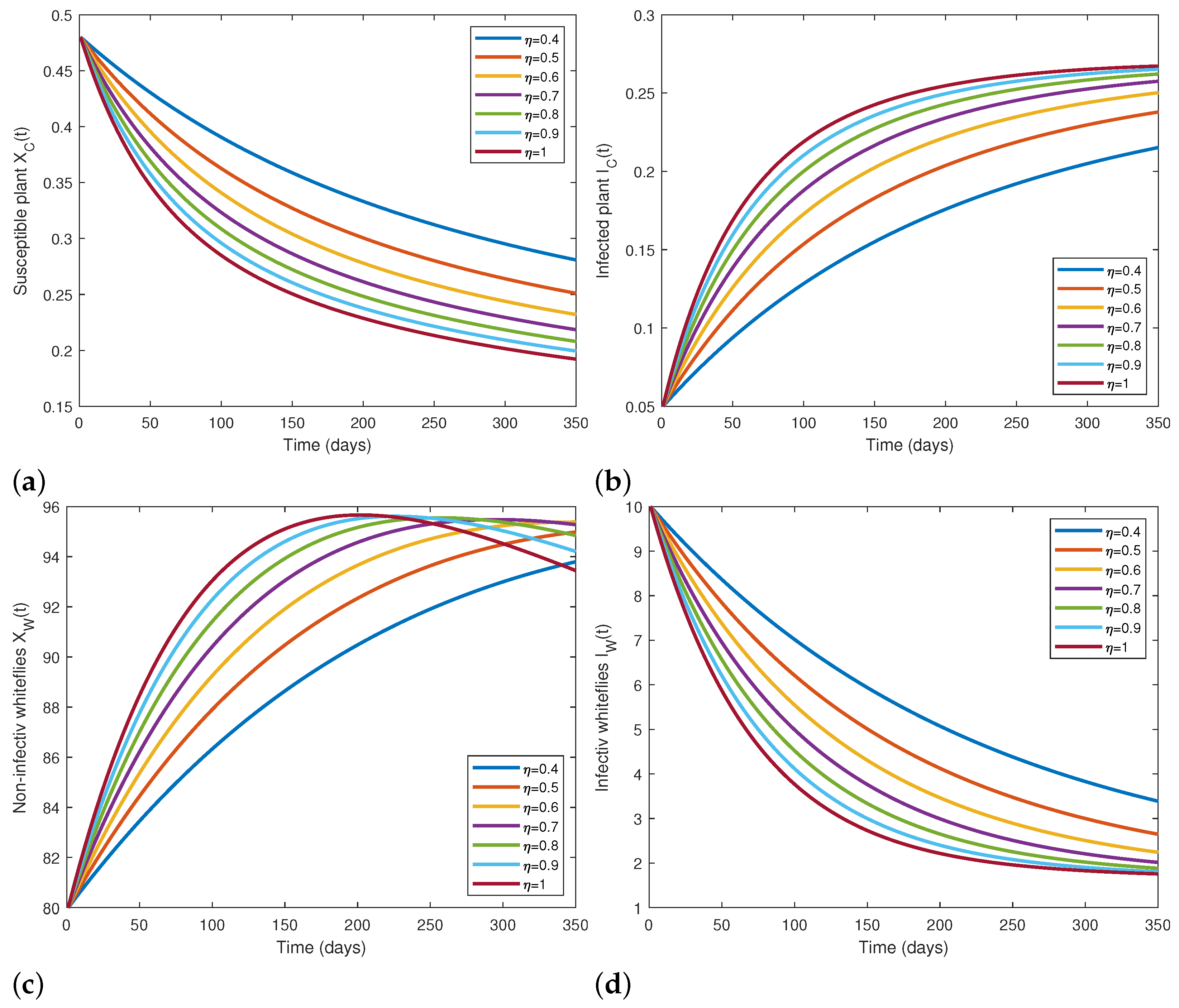
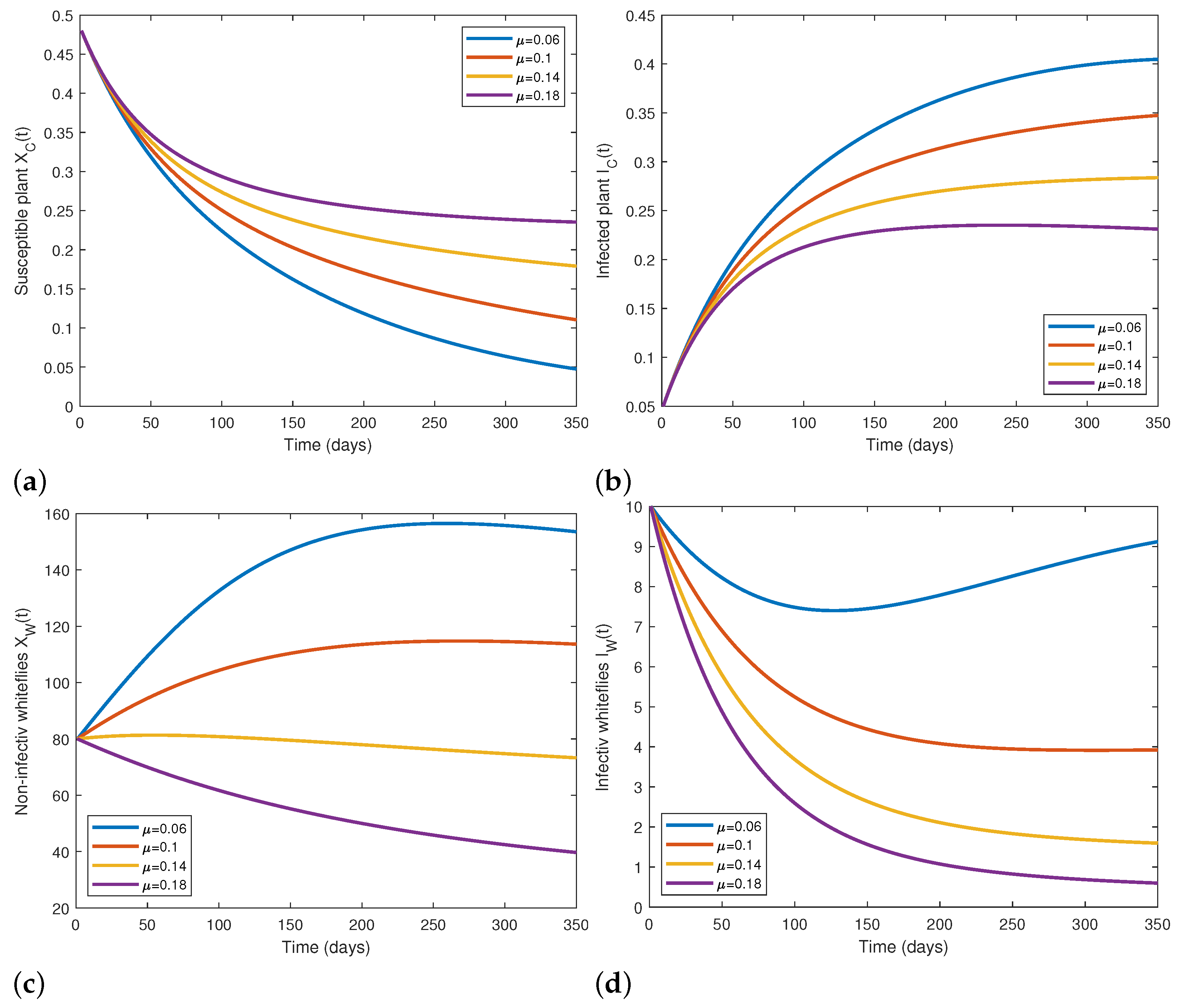
5.2. Numerical Simulations

In this part, we apply the numerical method that was shown in the previous Section 5.1 to provide numerical simulations for the CMD system (3). We obtain the predictor equations as the following

$$\begin{array}{cc}\hfill X_C^{P1}\left(t_{n+1}\right)=& X_C\left(t_n\right)+\left[{\displaystyle \frac{h\eta }{(2-\eta )\mathbb{T}\left(\eta \right)}}-{\displaystyle \frac{2(1-\eta )}{(2-\eta )\mathbb{T}\left(\eta \right)}}\right](a{X}_C\left(t_n\right)\left(1-{\displaystyle \frac{X_C\left(t_n\right)+I_C\left(t_n\right)}{k}}\right)\hfill \\ & +\beta I_C\left(t_n\right)-r{I}_W\left(t_n\right)X_C\left(t_n\right)-\psi X_C\left(t_n\right)),\hfill \\ \hfill X_C^{P2}\left(t_{n+1}\right)=& \left[{\displaystyle \frac{h\eta }{(2-\eta )\mathbb{T}\left(\eta \right)}}+{\displaystyle \frac{2(1-\eta )}{(2-\eta )\mathbb{T}\left(\eta \right)}}\right](a{X}_C\left(t_{n+1}\right)\left(1-{\displaystyle \frac{X_C\left(t_{n+1}\right)+I_C\left(t_{n+1}\right)}{k}}\right)\hfill \\ & +\beta I_C\left(t_{n+1}\right)-r{I}_W\left(t_{n+1}\right)X_C\left(t_{n+1}\right)-\psi X_C\left(t_{n+1}\right)),\hfill \end{array}$$

$$\begin{array}{cc}\hfill I_C^{P1}\left(t_{n+1}\right)=& I_C\left(t_n\right)+\left[{\displaystyle \frac{h\eta }{(2-\eta )\mathbb{T}\left(\eta \right)}}-{\displaystyle \frac{2(1-\eta )}{(2-\eta )\mathbb{T}\left(\eta \right)}}\right]\left(r{I}_W\left(t_n\right)X_C\left(t_n\right)-(\beta +g+\psi )I_C\left(t_n\right)\right),\hfill \\ \hfill I_C^{P2}\left(t_{n+1}\right)=& \left[{\displaystyle \frac{h\eta }{(2-\eta )\mathbb{T}\left(\eta \right)}}+{\displaystyle \frac{2(1-\eta )}{(2-\eta )\mathbb{T}\left(\eta \right)}}\right]\left(r{I}_W\left(t_{n+1}\right)X_C\left(t_{n+1}\right)-(\beta +g+\psi )I_C\left(t_{n+1}\right)\right),\hfill \\ \hfill X_W^{P1}\left(t_{n+1}\right)=& X_W\left(t_n\right)+\left[{\displaystyle \frac{h\eta }{(2-\eta )\mathbb{T}\left(\eta \right)}}-{\displaystyle \frac{2(1-\eta )}{(2-\eta )\mathbb{T}\left(\eta \right)}}\right](b\left[X_W\left(t_n\right)+I_W\left(t_n\right)\right]\hfill \\ & \times \left[1-{\displaystyle \frac{X_W\left(t_n\right)+I_W\left(t_n\right)}{\rho +\vartheta \left(X_C\left(t_n\right)+I_C\left(t_n\right)\right)}}\right]-m{I}_C\left(t_n\right)X_W\left(t_n\right)-\mu X_W\left(t_n\right)),\hfill \\ \hfill X_W^{P2}\left(t_{n+1}\right)=& \left[{\displaystyle \frac{h\eta }{(2-\eta )\mathbb{T}\left(\eta \right)}}+{\displaystyle \frac{2(1-\eta )}{(2-\eta )\mathbb{T}\left(\eta \right)}}\right](b\left[X_W\left(t_{n+1}\right)+I_W\left(t_{n+1}\right)\right]\hfill \\ & \times \left[1-{\displaystyle \frac{X_W\left(t_{n+1}\right)+I_W\left(t_{n+1}\right)}{\rho +\vartheta \left(X_C\left(t_{n+1}\right)+I_C\left(t_{n+1}\right)\right)}}\right]-m{I}_C\left(t_{n+1}\right)X_W\left(t_{n+1}\right)-\mu X_W\left(t_{n+1}\right)),\hfill \\ \hfill I_W^{P1}\left(t_{n+1}\right)=& I_W\left(t_n\right)+\left[{\displaystyle \frac{h\eta }{(2-\eta )\mathbb{T}\left(\eta \right)}}-{\displaystyle \frac{2(1-\eta )}{(2-\eta )\mathbb{T}\left(\eta \right)}}\right]\left(m{I}_C\left(t_n\right)X_W\left(t_n\right)-\mu I_W\left(t_n\right)\right),\hfill \\ \hfill I_W^{P2}\left(t_{n+1}\right)=& \left[{\displaystyle \frac{h\eta }{(2-\eta )\mathbb{T}\left(\eta \right)}}+{\displaystyle \frac{2(1-\eta )}{(2-\eta )\mathbb{T}\left(\eta \right)}}\right]\left(m{I}_C\left(t_{n+1}\right)X_W\left(t_{n+1}\right)-\mu I_W\left(t_{n+1}\right)\right).\hfill \end{array}$$

(68)

Therefore, the new corrector is given by

$$\begin{array}{cc}\hfill X_C\left(t_{n+1}\right)=& X_C^{P1}\left(t_{n+1}\right)+\left[{\displaystyle \frac{h\eta }{(2-\eta )\mathbb{T}\left(\eta \right)}}+{\displaystyle \frac{2(1-\eta )}{(2-\eta )\mathbb{T}\left(\eta \right)}}\right](a\left[X_C^{P1}\left(t_{n+1}\right)+X_C^{P2}\left(t_{n+1}\right)\right]\hfill \\ & \times \left(1-{\displaystyle \frac{\left[X_C^{P1}\left(t_{n+1}\right)+X_C^{P2}\left(t_{n+1}\right)\right]+\left[I_C^{P1}\left(t_{n+1}\right)+I_C^{P2}\left(t_{n+1}\right)\right]}{k}}\right)\hfill \\ & +\beta \left[I_C^{P1}\left(t_{n+1}\right)+I_C^{P2}\left(t_{n+1}\right)\right]-r\left[I_W^{P1}\left(t_{n+1}\right)+I_W^{P2}\left(t_{n+1}\right)\right]\left[X_C^{P1}\left(t_{n+1}\right)+X_C^{P2}\left(t_{n+1}\right)\right]\hfill \\ & -\psi \left[X_C^{P1}\left(t_{n+1}\right)+X_C^{P2}\left(t_{n+1}\right)\right]),\hfill \\ \hfill I_C\left(t_{n+1}\right)=& I_C^{P1}\left(t_{n+1}\right)+\left[{\displaystyle \frac{h\eta }{(2-\eta )\mathbb{T}\left(\eta \right)}}+{\displaystyle \frac{2(1-\eta )}{(2-\eta )\mathbb{T}\left(\eta \right)}}\right](r\left[I_W^{P1}\left(t_{n+1}\right)+I_W^{P2}\left(t_{n+1}\right)\right][X_C^{P1}\left(t_{n+1}\right)\hfill \\ & +X_C^{P2}\left(t_{n+1}\right)]-(\beta +g+\psi )\left[I_C^{P1}\left(t_{n+1}\right)+I_C^{P2}\left(t_{n+1}\right)\right]),\hfill \end{array}$$

$$\begin{array}{cc}\hfill X_W\left(t_{n+1}\right)=& X_W^{P1}\left(t_{n+1}\right)+\left[{\displaystyle \frac{h\eta }{(2-\eta )\mathbb{T}\left(\eta \right)}}-{\displaystyle \frac{2(1-\eta )}{(2-\eta )\mathbb{T}\left(\eta \right)}}\right][b[\left[X_W^{P1}\left(t_{n+1}\right)+X_W^{P2}\left(t_{n+1}\right)\right]\hfill \\ & +\left[I_W^{P1}\left(t_{n+1}\right)+I_W^{P2}\left(t_{n+1}\right)\right]]\hfill \\ & \times \left[1-{\displaystyle \frac{\left[X_W^{P1}\left(t_{n+1}\right)+X_W^{P2}\left(t_{n+1}\right)\right]+\left[I_W^{P1}\left(t_{n+1}\right)+I_W^{P2}\left(t_{n+1}\right)\right]}{\rho +\vartheta \left(\left[X_C^{P1}\left(t_{n+1}\right)+X_C^{P2}\left(t_{n+1}\right)\right]+\left[I_C^{P1}\left(t_{n+1}\right)+I_C^{P2}\left(t_{n+1}\right)\right]\right)}}\right]\hfill \\ & -m\left[I_C^{P1}\left(t_{n+1}\right)+I_C^{P2}\left(t_{n+1}\right)\right]\left[X_W^{P1}\left(t_{n+1}\right)+X_W^{P2}\left(t_{n+1}\right)\right]-\mu [X_W^{P1}\left(t_{n+1}\right)\hfill \\ & +X_W^{P2}\left(t_{n+1}\right)\left]\right],\hfill \end{array}$$

$$\begin{array}{cc}\hfill I_W\left(t_{n+1}\right)=& I_W^{P1}\left(t_{n+1}\right)+\left[{\displaystyle \frac{h\eta }{(2-\eta )\mathbb{T}\left(\eta \right)}}-{\displaystyle \frac{2(1-\eta )}{(2-\eta )\mathbb{T}\left(\eta \right)}}\right](m\left[I_C^{P1}\left(t_{n+1}\right)+I_C^{P2}\left(t_{n+1}\right)\right]\hfill \\ & \times \left[X_W^{P1}\left(t_{n+1}\right)+X_W^{P2}\left(t_{n+1}\right)\right]-\mu \left[I_W^{P1}\left(t_{n+1}\right)+I_W^{P2}\left(t_{n+1}\right)\right]).\hfill \end{array}$$

(69)

Here, we used the parameters shown in

Table 1. Parameters values cited from [48,49].

Parameter	Description	Value
a	The maximum replanting rate	0.05 day−1
k	The maximum abundance of cassava plant	0.5 m−2
$\beta$	The recovery rate of cassava plant	0.003 day−1
r	Infection rate	0.008 vector−1 day−1
$\psi$	The harvesting rate of cassava plant	0.003 day−1
g	Roguing/removed plant rate	0.003 day−1
b	The growth rate of whitefly vectors	0.2 day−1
$\alpha$	The external sources of infections	1 vector−1 day−1
$\vartheta$	The maximum abundance of vectors	500 plant−1
m	The rate of virus acquisition by non-infective vectors	0.008 plant−1 day−1
$\mu$	Death rate of whitefly vectors	0.12 day−1

to provide numerical simulations to illustrate the analytical findings of the proposed system (3). We used the proposed numerical method to perform the numerical simulation of CMD model dynamics using the parameters shown in Table 1 with time-step $h=0.1$ for a duration of 350 days that was appointed by setting the final time $t_{final}=35$. The initial condition values that were used in these simulations are $X_C\left(0\right)=0.48$, $I_C\left(0\right)=0.05$, $X_W\left(0\right)=80$, and $I_W\left(0\right)=10$. We used MATLAB R2021a programming to implement the numerical simulations of the proposed model.

Figure 1 shows the CMD model dynamics at various fractional orders $\eta =0.4,0.5,0.6,$$0.7,0.8,0.9$, and the integer order $\eta =1$ based on the actual parameters shown in Table 1. It also showed that the number of healthy cassava plants regularly decreases from 0.48 to 0.28 per m² at $\eta =0.4$ during 350 days. When the fractional order increases, the simulations show that the number of healthy cassava plants regularly decreases and ends up around 0.2 per m² at $\eta =1.$ The infected cassava plants regularly increase from 0.05 per m² to 0.23 per m² at $\eta =0.4$ during 350 days. When the fractional order increases, the simulations show that the number of infected cassava plants regularly increases and ends up around 0.27 per m² at $\eta =1$. The non-infected whitefly vectors had slowly increased from 80 to approximately 95 vectors per m² during the first 360 days for the fractional orders $\eta =0.4,0.5,0.6,$ and 0.7 with population increase with the increase in the fractional order. When the fractional order is near the value $\eta =1$, it is clear that the non-infected whitefly vectors had slowly increased from 80 to approximately 95 vectors per m² during the first 200 days and then started to decrease and became around 93 vectors per m². The infected whitefly vectors regularly decrease from 10 per m² to 3.5 per m² at $\eta =0.4$ during 350 days. When the fractional order increases, the simulations show that the number of infected whitefly vectors regularly decreases and ends up around 0.25 per m² at $\eta =1$.

Globally, the population of healthy cassava plants and infected whitefly vectors decreases when the fractional order decreases. In contrast, the infected cassava plant population and healthy whitefly vector population increases when the fractional order increases. For our numerical simulations, it is concluded that a small change in the fractional orders can cause an evident change in the dynamics of the CMD population. These differences allow for describing more accurately the behavior of the epidemic. Because the CMD model with ordinary derivatives cannot entirely investigate the spread of the virus and the total infected plants, the use of the fractional derivatives in the sense of a CF-operator allows for obtaining more accurate results to describe the dynamic behavior of the CMD model.

In Figure 2, we investigated CMD model dynamics at fractional order $\eta =0.9$, taking $\beta$ values between 0 and 0.02 with a step size of 0.005. When $\beta =0$, it indicates that there is no recovery rate among the infected cassava plant, whereas the value $\beta =0.02$ shows that the recovery rate of the infected cassava plant represents the maximum possible value of the recovery rate of the infected cassava plant [48]. The recovery rate made a clear positive impact of decreasing the density of infected cassava plants and prevented healthy cassava plants from getting infected. We concluded that when $\beta =0$, the density of healthy cassava plants decreases. In contrast, the density of infected cassava plants continuously increased. The non-infected whitefly vectors also increased, whereas the infected whitefly vectors slowly decreased. Although there is no recovery rate, the infected whitefly vectors are still decreasing; this decrease is due to the infection parameter ratio of the whitefly vectors being less than its mortality parameter value. In contrast, when $\beta =0.02$, we noticed that the density of healthy cassava plants slowly decreased, whereas the density of infected cassava plants slowly increased and became stable at 0.3 infected plants per m² after 150 days. The non-infected whitefly vectors increased, whereas the infected whitefly vectors quickly decreased. When the ratio of $\beta$ increases, CMD infections can be controlled, whereas when the ratio of $\beta$ decreases, CMD infections become difficult to be control.

In Figure 3, we investigated CMD model dynamics at fractional orders $\eta =0.9.$, taking $\mu$ values between 0.06 and 0.18 with a step size of 0.04. When $\mu =0.06$, it means that the mortality rate among the whitefly vectors is very small, whereas the value $\mu =0.18$ represents the maximum possible value of the mortality rate of whitefly vectors [48]. Whenever the mortality rate of whitefly vectors decreases, the number of infected and non-infected whitefly vectors decreases, causing more infection in healthy cassava plants. It also shows that when the mortality rate of whitefly vectors increases, the number of infected and non-infected whitefly vectors decreases, resulting in the stability of healthy cassava plants, making the control of CMD possible.

From the discussion above, it is concluded that the recovery rate, including treatment or roguing, or increasing the mortality rate of whitefly vectors, are both good strategies to control the spread of CMD in cassava fields. The figures also showed that increasing the mortality rate of whitefly vectors can control the infection better than increasing the recovery rate. This study suggests using some scientific strategies that were recommended in related studies and aimed to minimize the whitefly vector, which helps to control the CMD epidemic; for example, in [50], the researchers discussed the efficiency of cutting dipping in flupyradifurone for whitefly control and the influence of the mode of application on whitefly parasitism under farmer field conditions. They found that the insecticide treatment significantly reduced adult whiteflies by 41%, nymphs by 64%, and CMD incidence by 16%, and it increased root yield by 49%. Another study considered the seasonal land use changes that impacted whitefly Bemisia tabaci and its parasitoids in the agricultural landscape in Uganda [51]. They found that the dominant species of whitefly Bemisia tabaci on cassava was Sub-Saharan Africa 1 (SSA1), which was also found on some other neighboring crops and weeds. The highest abundance of whitefly Bemisia tabaci SSA1 nymphs in cassava fields occurred at times when landscapes had large areas of weeds, low to moderate areas of maize, and low areas of banana. Sarina et al. [52] provided management options to decrease whitefly abundance, including describing the features of landscapes with high parasitism. They found that the choice of cassava cultivar by the farmer is critical to reduce the whitefly epidemic risk at the landscape scale.

For improving the control strategies of CMD, future studies are recommended to add time delays into the model to capture the latency period between infection and the manifestation of symptoms in cassava plants or the time lag in response to control measures. Investigating the inclusion of seasonal variations can also reflect the periodic changes in environmental conditions, such as temperature and rainfall, which influence the growth rates of cassava plants and whitefly populations. Since real-world systems are subject to random fluctuations and uncertainties, incorporating stochastic terms into the model can help with studying the impact of environmental noise and random events on disease dynamics.

6. Conclusions

In this paper, we studied the dynamics of the fractional CMD model with the help of the corrector–predictor method in the sense of a Caputo–Fabrizio fractional derivative. With the help of fixed-point theory, we studied the existence of the unique solution of the CMD fractional model. Using the Picard iteration method, we performed stability analysis of the model. We proposed a corrector–predictor scheme for the CF-fractional derivative. This numerical scheme is strong and highly recommended in finding the solution to fractional models of physical, biological, and medical nonlinear fractional models in the sense of CF- derivatives. It is applied to obtain a numerical simulation of the CMD fractional model. Our results are helpful in figuring out the dynamics and behavior of the compartments of the model. For the epidemic model solution, we gave various graphical results at different values of fractional order and investigated the compartments’ behavior at different values of some important parameters. It concluded that the recovery rate, including treatment or roguing, or increasing the mortality rate of whitefly vectors, are both good strategies to control the spread of CMD in cassava fields. It also showed that increasing the mortality rate of whitefly vectors can control the infection better than increasing the recovery rate. Further study could explore how environmental factors and seasonal impacts might affect the prevalence and severity of CMD in order to develop more effective disease management strategies.

References

1. Rey, C.; Vanderschuren, H. Cassava mosaic and brown streak diseases: Current perspectives and beyond. Annu. Rev. Virol. 2017, 4, 429–452. [Google Scholar] [CrossRef]
2. Byju, G.; Suja, G. Mineral nutrition of cassava. Adv. Agron. 2020, 159, 169–235. [Google Scholar]
3. FAOSTAT FAO Statistics. Food and Agriculture Organization of the United Nations 2018. 2020. Available online: http://www.fao.org/faostat/en/ (accessed on 1 June 2018).
4. Tafesse, A.; Mena, B.; Belay, A.; Aynekulu, E.; Recha, J.W.; Osano, P.M.; Darr, D.; Demissie, T.D.; Endalamaw, T.B.; Solomon, D. Cassava production efficiency in southern Ethiopia: The parametric model analysis. Front. Sustain. Food Syst. 2021, 5, 758951. [Google Scholar] [CrossRef]
5. Legg, J.; Winter, S. Cassava mosaic viruses (Geminiviridae). In Reference Module in Life Sciences; Elsevier: Amsterdam, The Netherlands, 2020; Volume 2020, pp. 1–12. [Google Scholar]
6. Al-Basir, F.; Banerjee, A.; Ray, S. Role of farming awareness in crop pest management—A mathematical model. J. Theor. Biol. 2019, 461, 59–67. [Google Scholar] [CrossRef]
7. Chowdhury, J.; Al-Basir, F.; Takeuchi, Y.; Ghosh, M.; Roy, P.K. A mathematical model for pest management in Jatropha curcas with integrated pesticides-An optimal control approach. Ecol. Complex. 2019, 37, 24–31. [Google Scholar] [CrossRef]
8. Melese, A.S.; Makinde, O.D.; Obsu, L.L. Mathematical modelling and analysis of coffee berry disease dynamics on a coffee farm. Math. Biosci. Eng. 2022, 19, 7349–7373. [Google Scholar] [CrossRef]
9. Tabonglek, S.; Humphries, U.W.; Khan, A. Mathematical Model for Rice Blast Disease Caused by Spore Dispersion Affected from Climate Factors. Symmetry 2022, 14, 1131. [Google Scholar] [CrossRef]
10. Blyuss, K.B.; Al-Basir, F.; Tsygankova, V.A.; Biliavska, L.O.; Iutynska, G.O.; Kyrychko, S.N.; Dziuba, S.V.; Tsyliuryk, O.I.; Izhboldin, O. Control of mosaic disease using microbial biostimulants: Insights from mathematical modelling. Ric. Mat. 2020, 69, 437–455. [Google Scholar] [CrossRef]
11. Atanasov, A.; Georgiev, S.; Vulkov, L. Numerical Analysis of the Transfer Dynamics of Heavy Metals from Soil to Plant and Application to Contamination of Honey. Symmetry 2024, 16, 110. [Google Scholar] [CrossRef]
12. Al-Basir, F.; Ray, S. Impact of farming awareness based roguing, insecticide spraying and optimal control on the dynamics of mosaic disease. Ric. Mat. 2020, 69, 393–412. [Google Scholar] [CrossRef]
13. Al-Basir, F.; Roy, P.K. Dynamics of mosaic disease with roguing and delay in Jatropha curcas plantations. J. Appl. Math. Comput. 2018, 58, 1–31. [Google Scholar] [CrossRef]
14. Rakshit, N.; Al-Basir, F.; Banerjee, A.; Ray, S. Dynamics of plant mosaic disease propagation and the usefulness of roguing as an alternative biological control. Ecol. Complex. 2019, 38, 15–23. [Google Scholar] [CrossRef]
15. Al-Basir, F.; Kyrychko, Y.N.; Blyuss, K.B.; Ray, S. Effects of vector maturation time on the dynamics of cassava mosaic disease. Bull. Math. Biol. 2021, 83, 1–21. [Google Scholar] [CrossRef]
16. Maity, S.; Mandal, P.S. A comparison of deterministic and stochastic plant-vector-virus models based on probability of disease extinction and outbreak. Bull. Math. Biol. 2022, 84, 1–41. [Google Scholar] [CrossRef] [PubMed]
17. Jittamai, P.; Chanlawong, N.; Atisattapong, W.; Anlamlert, W.; Buensanteai, N. Reproduction number and sensitivity analysis of cassava mosaic disease spread for policy design. Math. Biosci. Eng. 2021, 18, 5069–5093. [Google Scholar] [CrossRef]
18. Ahmed, I.; Kiataramkul, C.; Muhammad, M.; Tariboon, J. Existence and Sensitivity Analysis of a Caputo Fractional-Order Diphtheria Epidemic Model. Mathematics 2024, 12, 2033. [Google Scholar] [CrossRef]
19. Subramanian, S.; Kumaran, A.; Ravichandran, S.; Venugopal, P.; Dhahri, S.; Ramasamy, K. Fuzzy Fractional Caputo Derivative of Susceptible-Infectious-Removed Epidemic Model for Childhood Diseases. Mathematics 2024, 12, 466. [Google Scholar] [CrossRef]
20. Atangana, A.; Baleanu, D.; Alsaedi, A. Analysis of time-fractional Hunter-Saxton equation: A model of neumatic liquid crystal. Open Phys. 2016, 14, 145–149. [Google Scholar] [CrossRef]
21. Fahad, A.; Boulaaras, S.M.; Rehman, H.U.R.; Iqbal, I.; Saleem, M.S.; Chou, D. Analysing soliton dynamics and a comparative study of fractional derivatives in the nonlinear fractional Kudryashov’s equation. Results Phys. 2023, 55, 107114. [Google Scholar] [CrossRef]
22. Li, J.F.; Ahmad, I.; Ahmad, G.; Shah, D.; Chu, U.M.; Thounthong, P.; Ayaz, M. Numerical solution of two-term time-fractional PDE models arising in mathematical physics using local meshless method. Open Phys. 2020, 18, 1063–1072. [Google Scholar] [CrossRef]
23. Atangana, A.; Baleanu, D. Caputo-Fabrizio derivative applied to groundwater flow within confined aquifer. J. Eng. Mech. 2017, 143, D4016005. [Google Scholar] [CrossRef]
24. Khan, A.; Abdeljawad, T.; Gomez-Aguilar, J.F.; Khan, H. Dynamical study of fractional order mutualism parasitism food web module. Chaos Solit. Fractals 2020, 134, 109685. [Google Scholar] [CrossRef]
25. Khan, A.; Gomez-Aguilar, J.F.; Abdeljawad, T.; Khan, H. Stability and numerical simulation of a fractional order plant-nectar-pollinator model. Alex. Eng. J. 2020, 59, 49–59. [Google Scholar] [CrossRef]
26. Hussain, S.; Madi, E.N.; Iqbal, N.; Botmart, T.; Karaca, Y.; Mohammed, W.W. Fractional dynamics of vector-borne infection with sexual transmission rate and vaccination. Mathematics 2021, 9, 3118. [Google Scholar] [CrossRef]
27. Cao, X.; Ghosh, S.; Rana, S.; Bose, H.; Roy, P.K. Application of an Optimal Control Therapeutic Approach for the Memory-Regulated Infection Mechanism of Leprosy through Caputo-Fabrizio Fractional Derivative. Mathematics 2023, 11, 3630. [Google Scholar] [CrossRef]
28. Thabet, S.T.M.; Abdo, M.S.; Shah, K.; Abdeljawad, T. Study of transmission dynamics of COVID-19 mathematical model under ABC fractional order derivative. Results Phys. 2020, 19, 103507. [Google Scholar] [CrossRef] [PubMed]
29. Begum, R.; Tunç, O.; Khan, H.; Gulzar, H.; Khan, A. A fractional order Zika virus model with Mittag-Leffler kernel. Chaos Solit. Fractals 2021, 146, 110898. [Google Scholar] [CrossRef]
30. Shah, N.; Nor, H.; Jan, R.; Ahmad, H.; Razak, N.N.A.; Ahmad, I.; Ahmad, H. Enhancing public health strategies for tungiasis: A mathematical approach with fractional derivative. AIMS Bioeng. 2023, 10, 384–405. [Google Scholar] [CrossRef]
31. Noeiaghdam, S.; Micula, S.; Nieto, J.J. A novel technique to control the accuracy of a nonlinear fractional order model of COVID-19: Application of the CESTAC method and the CADNA library. Mathematics 2021, 9, 1321. [Google Scholar] [CrossRef]
32. Tomasiello, S.; Macías-Díaz, J.E. A Mini-Review on Recent Fractional Models for Agri-Food Problems. Mathematics 2023, 11, 2316. [Google Scholar] [CrossRef]
33. Abdullah, T.Q.S.; Huang, G.; Al-Sadi, W. A curative and preventive treatment fractional model for plant disease in Atangana-Baleanu derivative through Lagrange interpolation. Int. J. Biomath. 2022, 15, 2250052. [Google Scholar] [CrossRef]
34. Guo, W.; Campanella, O.H. A relaxation model based on the application of fractional calculus for describing the viscoelastic behavior of potato tubers. Trans. ASABE 2017, 60, 259–264. [Google Scholar]
35. Achar, S.J.; Baishya, C.; Veeresha, P.; Akinyemi, L. Dynamics of fractional model of biological pest control in tea plants with Beddington–DeAngelis functional response. Fractal Fract. 2021, 6, 1. [Google Scholar] [CrossRef]
36. Liu, S.; Huang, M.; Wang, J. Bifurcation control of a delayed fractional Mosaic disease model for Jatropha curcas with farming awareness. J. Complex. 2020, 2020, 2380451. [Google Scholar] [CrossRef]
37. Kumar, P.; Erturk, V.S.; Almusawa, H. Mathematical structure of mosaic disease using microbial biostimulants via Caputo and Atangana-Baleanu derivatives. Results Phys. 2021, 24, 104186. [Google Scholar] [CrossRef]
38. Kumar, P.; Erturk, V.S.; Almusawa, H. Dynamic analysis and bifurcation control of a fractional-order cassava mosaic disease model. J. Appl. Math. Comput. 2023, 69, 1705–1730. [Google Scholar]
39. Achar, S.J.K.; Geetha, N. Dynamics of fractional plant virus propagation model with influence of seasonality and intraspecific competition. Math. Methods Appl. Sci. 2024, 47, 6415–6430. [Google Scholar] [CrossRef]
40. Ghalib, M.M.; Zafar, A.A.; Hammouch, Z.; Riaz, M.B.; Shabbir, K. Analytical results on the unsteady rotational flow of fractional-order non-newtonian fluids with shear stress on the boundary. Discret. Contin. Dyn. Syst.-S 2020, 13, 683. [Google Scholar]
41. Caputo, M.; Fabrizio, M. A new definition of fractional derivative without singular kernel. Prog. Fract. Differ. Appl. 2015, 1, 73–85. [Google Scholar]
42. Kilbas, A.A.; Srivastava, H.M.; Trujillo, J.J. Theory and Applications of Fractional Differential Equations; Elsevier: Amsterdam, The Netherlands, 2006; Volume 204. [Google Scholar]
43. Losada, J.; Nieto, J.J. Properties of a new fractional derivative without singular kernel. Prog. Fract. Differ. Appl. 2015, 1, 87–92. [Google Scholar]
44. Wang, J.; Zhou, Y.; Medved, M. Picard and weakly Picard operators technique for nonlinear differential equations in Banach spaces. J. Math. Anal. Appl. 2012, 389, 261–274. [Google Scholar] [CrossRef]
45. Baleanu, D.; Mohammadi, H.; Rezapour, S. A fractional differential equation model for the COVID-19 transmission by using the Caputo-Fabrizio derivative. Adv. Differ. Equ. 2020, 2020, 299. [Google Scholar] [CrossRef] [PubMed]
46. Mahatekar, Y.; Scindia, P.S.; Kumar, P. A new numerical method to solve fractional differential equations in terms of Caputo-Fabrizio derivatives. Phys. Scr. 2023, 98, 024001. [Google Scholar] [CrossRef]
47. Daftardar-Gejji, V.; Jafari, H. An iterative method for solving nonlinear functional equations. J. Math. Anal. Appl. 2006, 316, 753–763. [Google Scholar] [CrossRef]
48. Holt, J.; Jeger, M.J.; Thresh, J.M.; Otim-Nape, G.W. An epidemilogical model incorporating vector population dynamics applied to African cassava mosaic virus disease. J. Appl. Ecol. 1997, 34, 793–806. [Google Scholar] [CrossRef]
49. Santra, N.; Sahoo, D.; Mondal, S.; Samanta, G. An epidemiological multi-delay model on cassava mosaic disease with delay-dependent parameters. Filomat 2023, 37, 2887–2921. [Google Scholar] [CrossRef]
50. Caspary, R.; Wosula, E.N.; Issa, K.A.; Amour, M.; Legg, J.P. Cutting dipping application of Flupyradifurone against cassava whiteflies Bemisia tabaci and impact on its parasitism in cassava. Insects 2023, 14, 796. [Google Scholar] [CrossRef] [PubMed]
51. Kalyebi, A.; Macfadyen, S.; Hulthen, A.; Ocitti, P.; Jacomb, F.; Tay, W.T.; Colvin, J.; De Barro, P. Within-season changes in land-use impact pest abundance in smallholder African cassava production systems. Insects 2021, 12, 269. [Google Scholar] [CrossRef]
52. Macfadyen, S.; Tay, W.K.; Hulthen, A.D.; Paull, C.; Kalyebi, A.; Jacomb, F.; Parry, H.; Sseruwagi, P.; Seguni, Z.; Omongo, C.A.; et al. Landscape factors and how they influence whitefly pests in cassava fields across East Africa. J. Landsc. Ecol. 2021, 36, 45–67. [Google Scholar] [CrossRef]
Figure 1. Numerical simulation for the dynamics of CMD fractional model via the CF-derivative for η = 0.4 , 0.5 , 0.6 , 0.7 , 0.8 , 0.9 , 1 based on the parameters shown in Table 1. Here, (a) describes the dynamics of the susceptible cassava plant, (b) describes the dynamics of the infected cassava plant, (c) describes the dynamics of non-infective whiteflies, and (d) describes the dynamics of infective whiteflies.
Mathematics 12 02386 g001
Figure 2. Numerical simulation for the dynamics of the CMD model via the CF-fractional derivative for η = 0.9 , based on the parameters shown in Table 1 taking β values between 0 and 0.02 with a step-size of 0.005. Here, (a) describes the influence of recovery rate changes in the susceptible cassava plant population, (b) describes the influence of recovery rate changes in the infected cassava plant population, (c) describes the influence of recovery rate changes in the non-infective whiteflies population, and (d) describes the influence of recovery rate changes in the infective whiteflies population.
Mathematics 12 02386 g002
Figure 3. Numerical simulatio for the dynamics of CMD model via the CF-fractional derivative for = 0.9 based on the parameters shown in Table 1 with taking μ values between 0 and 0.25 with a step size of 0.05. Here, (a) describes the influence of whiteflies death rate changes in the susceptible cassava plant population, (b) describes the influence of whiteflies death rate changes in the infected cassava plant population, (c) describes the influence of whiteflies death rate changes in the non-infective whiteflies population, and (d) describes the influence of whiteflies death rate changes in the infective whiteflies population.
Mathematics 12 02386 g003