Article

A Discrete Resistance Network Based on a Multiresolution Grid for 3D Ground-Return Current Forward Modeling

1
School of Computer, Hubei University of Education, Wuhan 430205, China
2
School of Economics and Business Administration, Chongqing University, Chongqing 400044, China
3
Hubei Key Laboratory of Digital Finance Innovation, Hubei University of Economics, Wuhan 430205, China
4
School of Information Engineering, Hubei University of Economics, Wuhan 430205, China
5
State Key Laboratory of Power Transmission Equipment Technology, Chongqing University, Chongqing 400044, China
6
School of Resources and Safety Engineering, Chongqing University, Chongqing 400044, China
7
Hubei Internet Finance Information Engineering Technology Research Center, Hubei University of Economics, Wuhan 430205, China
*
Authors to whom correspondence should be addressed.
Mathematics 2024, 12(15), 2392; https://doi.org/10.3390/math12152392 (registering DOI)
Submission received: 7 July 2024 / Revised: 24 July 2024 / Accepted: 30 July 2024 / Published: 31 July 2024

Abstract

:
While the high-voltage direct current (HVDC) transmission system is in monopolar operation, it produces thousands of amperes of ground-return currents (GRCs). Accurate computation of the GRCs is essential for assessing safety implications for nearby industrial infrastructure. Current three-dimensional forward models of GRCs are typically constructed based on discrete differential equations, and their solving efficiency is constrained by the increased degrees of freedom resulting from the fine discretization grids in high-conductivity conductors and ground points. To address this issue, we present a new resistor network (RN) forward solver based on a multi-resolution grid approach. This solver utilizes an RN to avoid the massive degrees of freedom resulting from fine discretization of high-voltage conductors and enhances grid discretization efficiency near the surface grounding system through multi-resolution grids. We demonstrate, through multiple three-dimensional geoelectrical model cases, that the proposed method reduces the forward modeling misfit to 1% and possesses only 3‰ of the required discrete elements compared to traditional approaches. Furthermore, practical HVDC grid model analyses indicate the successful application of the proposed method for GRC analysis in complex geoelectric conditions.

1. Introduction

High-voltage direct current (HVDC) is suitable for projects involving the transmission of substantial power over extended distances. Due to the special erection and operation mode of HVDC transmission lines, when they are in a monopolar operation state, they inject high-power direct current (DC) into the ground, generating ground-return currents (GRCs) and earth surface potentials (ESPs) [1,2]. Unconsidered industrial stray current flowing into an alternating current (AC) power grid is harmful to power grid equipment, particularly if it leads to DC bias in transformer equipment. Therefore, accurate calculation of a substation’s neutral point current is crucial for the safe operation of AC/DC power grids [3,4].
Computing current and potential is a typical DC propagation problem [5] that is commonly solved via partial differential equation methods, represented by the moment method [6] and the finite element method (FEM) [7,8,9]. However, these differential methods struggle to discretize elongated, high-conductivity conductors, which can result in a massive system of differential equations with many degrees of freedom. Considering that these methods ignore the shunt effect of the overhead lines on the current and generate the solving misfit of the potential and neutral current, the resistance network (RN) method was developed [2,10]. Based on this, Kirchhoff’s resistance network was introduced, which constructs node current and voltage conservation equations for each differential unit [11]. This resistance-network-based differential discretization method avoids the problem of discretizing high-conductivity conductors encountered with traditional differential methods and is suitable for calculating problems involving long, straight conductors, steel casings, and ground electrical structures [11,12].
Building on Kirchhoff’s resistance network method, we utilized the node voltage (NV) principle [13] to construct a symmetric matrix system that includes both current conservation and voltage conservation equations. This system not only retains all unit information but also offers superior solving efficiency. However, the commonly used mesh for this system is relatively simple, primarily consisting of hexahedra. Using traditional structured grids to accurately represent rapid changes near the surface requires complex discretization, leading to increased computational costs due to the richness of the structured grid. The multiresolution (MR) grids presented in [14,15] strike a balance by employing primarily structured hexahedrons complemented by localized refinement based on nonconforming cells. This approach to grid construction enables adaptable resolution within a fundamentally structured grid, ensuring consistent mesh aspect ratios and enhancing the efficiency of grid discretization.
Following this introduction, Section 2 introduces the principles of the GRC. The proposed 3D RN based on MR grids is elaborated, including the processing of hanging nodes, boundary conditions, and grounding nodes, in Section 3. Section 4 contains numerical examples and analysis related to power grid applications, respectively. In Section 5, we draw our final conclusions regarding this work.

2. Related Works

2.1. Background

In this section, we introduce some basic concepts and principles of GRC and describe how the current during HVDC monopole operation propagates underground and leads to surface potential distribution. Additionally, we present the governing equations for this current propagation problem.
For initial cost considerations during the construction phase of the HVDC project, the system operated in a monopolar grounding configuration for several months until the activation of the second pole. Moreover, during HVDC monopole faults or maintenance periods, the system adopts asymmetric and monopolar operation modes in which the DC enters the earth through a circuit. Current enters the earth through one grounding electrode and exits from the grounding electrode at the opposite end. The generation of GRC occurs during HVDC monopolar operation, with DC ground currents (Figure 1) reaching up to thousands of amps [1].
When calculating a ground electrical model with an overhead power line above it (Figure 2), the shunting characteristics of the power line can alter the distribution of underground currents. This represents a typical field-circuit coupling problem. We calculate the resistance of the power line based on its length and cross-sectional area and integrate this resistance with the circuit representing the ground electrical structure to form a complete circuit for solving the field-circuit coupling problem. Since the computational model area is relatively small, this field-circuit coupling model can be discretized using the RN method. For larger research areas with significant longitudinal and transverse dimensions, this study employs a multi-resolution approach to establish a volumetric circuit model based on anisotropic meshes. This model allows for the flexible extension of the computational area, making it suitable for large-scale calculations over tens to hundreds of kilometers.
According to the law of conservation of charge, when the bulk charge density is 0, the differential form of the current continuity equation can be expressed as
j = 0 ,
where the current density j can be divided into the known current density j1 and the unknown current density j2.
Considering the interplay among the current density, electric field E, potential φ, and conductivity σ, i.e., j = σE and E =φ [16], we can obtain the following:
( σ φ ) = 0 ,

2.2. GRC Calculation

Computing current and potential is a typical DC propagation problem [5] that is commonly solved via partial differential equation methods, including the moment method, the finite element method (FEM), the finite difference method, and the finite volume method. The simulation of current and potential distribution in DC propagation problems is commonly addressed using methods based on partial differential equations. These include the moment method [6], the finite element method (FEM) [7,8,9,17,18], the finite difference method [19], and the finite volume method [20]. Considering that these methods ignore the shunt effect of the overhead lines on the current and generate the solving misfit of the potential and neutral current, the resistance network (RN) method was developed [2,10]. It views the ground as a horizontal layered and a vertical layered medium to construct the equivalent resistance [21,22,23] and realizes the forward simulation of GRCs.

2.3. Discrete Grid

To address the inadequacy of the RN method in accurately simulating the propagation of GRC in a 3D geoelectric structure, a structured hexahedral unit-based RN was developed [2]. This type of structured grid (SG) is commonly used in numerical simulation methods such as the finite difference method [24,25] and FEM [26,27,28]. The grids are relatively simple and mostly hexahedral. However, achieving accurate representation of swift variations near the surface using conventional regular grids necessitates intricate discretization, resulting in escalated computational expenses attributed to the abundance of structured grids [29,30].
Due to flexible dispersion performance, the unstructured grid can dissect the target area in a targeted manner and avoid the transitional dissection and dispersion of non-target areas such as the structured grid. Unstructured grids, encompassing hexahedrons and having garnered significant attention in the past decade, find application in the finite volume method [31,32] and FEM [33,34]. A tetrahedron can be used to fit complex underground electrical structures, but the calculation accuracy is closely related to the mesh quality. The quality of the tetrahedrons is uncontrollable and can generate narrow elements, resulting in poor mesh quality [35,36].
Unstructured grids relying on hexahedrons pose several challenges, including the complexity of mesh setup, the risk of matrix ill-conditioning arising from unfavorable aspect ratios, and necessity for additional postprocessing efforts [37].

2.4. Contributions

We introduce a multiresolution grid to the node voltage network for a more efficient discretization of underground structures. This method offers the following advantages:
(1)
The proposed resistance network system does not require the continuity of regular elements to establish an equipotential surface for circulating currents on a face, and it maintains good symmetry, resulting in higher solving efficiency.
(2)
The grid is refined at the source point and near the surface to enhance accuracy. This helps avoid redundant elements caused by lateral extension in regular grid refinement, reduces the degrees of freedom, and improves the solving efficiency of the resistance network system.
(3)
For hanging nodes in a multiresolution grid’s discretized resistance network, we compared three different interpolation methods and determined that the ghost fine interpolation resistance value method is suitable for MR resistance network discretization.

3. 3D RN Method

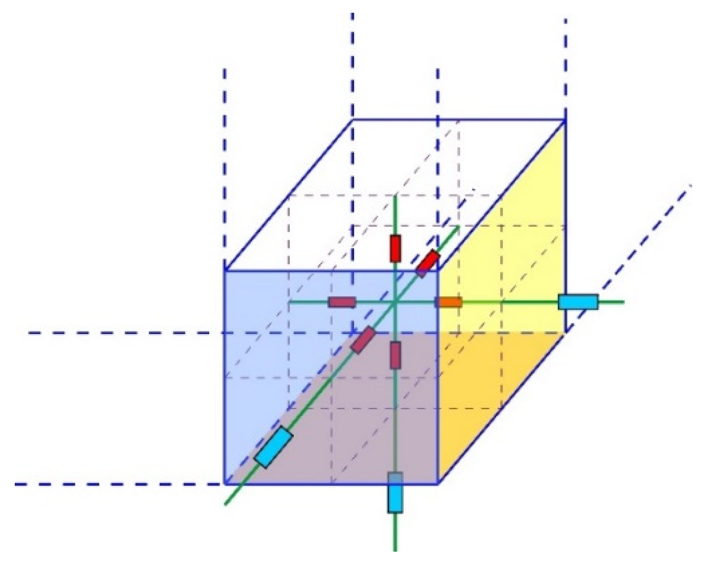
3.1. Stereo NV-RN on an SG

The integral form of Equation (2) can be expressed discretely as
( I 1 + I 2 ) = 0 ,
where I1 is a vector composed of currents on all current inflow nodes, and I2 is a vector composed of currents on all currents flowing out of nodes. This equation shows that the law of conservation of charge can fully derive Kirchhoff’s current law in electrical circuits under steady conditions. Considering that most HVDC grounding currents are DC or quasi-DC with very low frequency, when DC current propagates in the soil, it is usually affected only by the resistive effect of the soil. This resistance effect is equivalent to the blocking effect of the resistance element in the circuit on the current passing through it.
Taking node p as an example, it is specified that the current flows from node p into the other six subsidiary nodes, and the following can be obtained:
Y N × N U N × 1 = I N × 1 ,
Y N × N = [ Y p q ] U N × 1 = [ U p ] I N × 1 = [ i p ] N × 1 p = 1 , 2 , , N q = 1 , 2 , , N ,
here, p takes values from 1 to N, and q ranges from 1 to N, where N is the total number of cell nodes. In the node admittance matrix Y, the matrix elements are self-admittance when p = q, and the matrix elements are mutual admittance when pq. When the q-th node is not an adjacent subordinate node of the p-th node, the mutual admittance is 0. Therefore, the node admittance matrix exhibits sparsity and symmetry, with the width of the matrix remaining fixed based on a determined number of elements and the sorting method.
Obtaining the resistance between nodes is a necessary condition for using the node element method. Each regular hexahedral soil block is regarded as an independent unit, and the center of the unit is used as the potential sampling point. For a linear geoelectric case, the potential gradient of the grid boundary surface adopts the central difference format:
φ r + 1 / 2 = φ r + 1 φ r h r + 1 / 2 + O ( Δ h 2 ) r = i , j , k ,
where hr+1/2 = (hr + hr+1)/2 represents the average length of the grid edges of two adjacent cells in the axial direction.

3.2. MR Grid

MR grids offer an uncomplicated method for sparse data representation, utilizing fewer voxels for areas exhibiting minimal variability and a greater number of voxels for regions characterized by high variability. Unlike the structured SG grid, the MR grid has spatial recursive properties. The coarse grid is composed of multiple subgrids, as follows:
N g r i d = i = 1 N s N x C L ( i ) × N y C L ( i ) × N z C L ( i ) ,
where Ngrid denotes the total count of geoelectric cells. The coarseness level is represented by the coarseness parameter CL(i), i = 1, 2, …, Ns. Here, CL is positively related to the grid spacing and can be assigned values of 1, 2, 3, and the like, and the minimum coarseness level is 1, represented by CL(1) = 1. The subgrids are composed of structured grids with dimensions NxCL(i) × NyCL(i) × NzCL(i), and the multilevel recursion is formed after subdivision. The difference in the coarseness level between adjacent coarseness level grids is unique, so the MR grid can be established by using a basic refined grid and the variables [CL(i), Sp(i)], where Sp represents the subgrid spacing, and [CL, Sp] = [1, 5; 2, 10] provides a straightforward instance of an MR grid with a recursion depth of 2, as depicted in Figure 3.

3.3. MR Stereo NV-RN

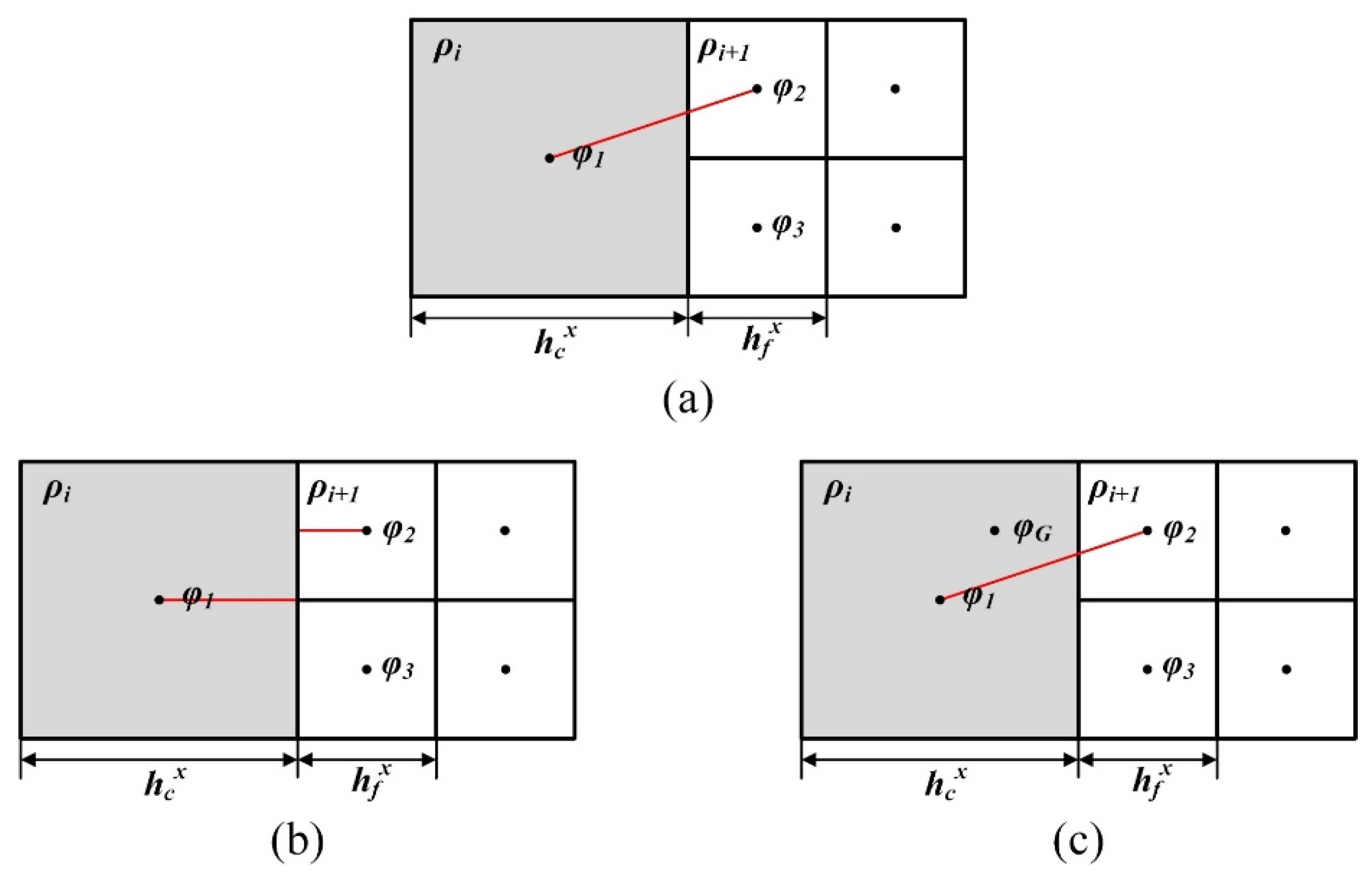
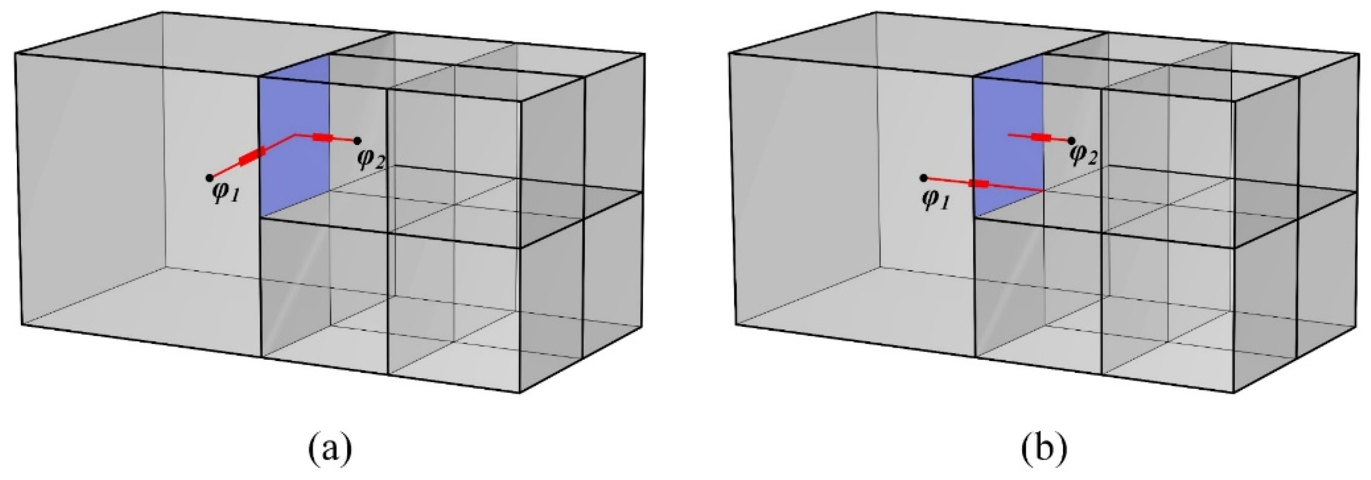
3.3.1. Hanging Nodes

The resistance value of the subgrids with the same CL is the same as that of the structured grid, and the mesh interface between adjacent CLs generates hanging nodes and hanging surfaces. Using Figure 4a as an example, the CL of cell 1 is larger than that of cells 2, 3, 4, and 5. Nodes nl, n2, n3, and n4 are so-called hanging nodes.
The hanging surface delineates the interface between coarse and fine meshes. In the process of electromagnetic flux numerical simulation based on MR grids, the fine grid surfels are obtained via the interpolation of coarse grid surfels, and fine mesh surfels are omitted from the system matrix. Using the same volumetric flux discretization as the structured grid, we obtain the following:
V i , j , k σ ( m ) φ n d S = S i , j , k ( σ ( m ) φ ) d S r = i , j , k Δ h = ± 1 2 σ ( m ) φ r + Δ h w r + Δ h S r + Δ h ,
where ω is the interpolation matrix.
When addressing the gradient operator at the junction of coarse and fine grids, using the x-direction refinement in Figure 4a as an example, the most natural method [38] is to approximate the gradient at the interface adjacent to the hierarchical grid as follows:
( φ ) x 2 φ 2 φ 1 h 2 - 1 ,
where h2-1 is the distance between nodes in the x-axis of the coarse and refined grids. We use the grid spacing hc of the coarse grid as the benchmark. Then, the finite difference of Equation (9) around the interface remains incomplete. Therefore, the formula may not even offer first-order accuracy.
Three types of grid spacing are defined in Figure 5: coarse spacing (CS), fine spacing (FS), and ghost fine (GF) spacing. The difference method is set to a coarse spacing (CS) grid (Figure 5a). We substitute Equation (9) into Equation (8), and the resistance coefficient between coarse and refined grids can be derived through surface interpolation.

3.3.2. Hanging Node Interpolation

We finally obtain the resistance relation between grids 1 and 2 as follows:
R i + 1 / 2 , j , k ( 1 ) = 3 4 ρ i + 1 / 2 , j , k h c x S i + 1 / 2 , j , k ,
where ρi+1/2,j,k = W1ρi,j,k + W2ρi+1,j,k and W is the volume-weighted average operator. The 3D equivalent resistance connection is shown in Figure 6a.
The grid spacing size can be reduced to improve the difference accuracy. The resistance between the two nodes can be determined by connecting the resistance of the coarse and refined grids on either side of the interface. The resistance of the coarse grid is determined by the spacing size hc, and for the refined grid, it is based on the spacing size hf, designated as the FS grid (Figure 6b). The setting method for setting the 3D equivalent resistance, followed by the equation, is illustrated in Figure 6.
R i , j , k = 1 2 ρ i , j , k h c x S i , j , k R i + 1 , j , k ( 1 ) = 1 2 ρ i + 1 , j , k h f x S i + 1 , j , k ,
After connecting two resistors in series, we obtain the following:
R i + 1 / 2 , j , k = R i , j , k + R i + 1 , j , k ( 1 ) ,
By referring to the difference method in [39], a higher-order precision approximation is used, and the Taylor series expansion directly at φ2 is not considered, but a ghost point is introduced, and the potential gradient is obtained through second-order precision interpolation. The interface gradient is approximated as follows:
( φ ) x 2 φ 1 + φ 2 2 φ 3 3 h f x ,
This seems to be the approximate value of the first-order accuracy O(h), but it was shown in [39] that the method actually offers second-order accuracy O(h2). We substituted Equation (13) into Equation (8) and obtained the resistance coefficient between coarse and refined grids through surface interpolation (Figure 5c), which is referred to as the GF. Finally, we obtained the relationship coefficients at the hanging nodes of adjacent coarse and fine grids in the Cartesian coordinate system to determine the resistance coefficient connected between grids 1 and 2 as follows:
R i + 1 / 2 , j , k ( 1 ) = 6 ρ i + 1 / 2 , j , k h f x S i + 1 / 2 , j , k

3.3.3. Boundary Conditions

Our network automatically truncates at the ground–air boundary to ensure that current does not flow from underground into the air (Figure 7). For the underground boundary, we did not use a complete uniform Dirichlet boundary. Instead, we added a resistance with a value lower than that of the boundary inside, simulating the effect of an infinite range on the current in the computation area.
To avoid difficulties in determining resistances on co-planar edge boundaries, our computational cells use the cell-centered method rather than the vertex-centered method. This approach limits our ability to compute surface voltages, providing only the voltage at a depth of half the cell’s vertical dimension underground. However, since the neutral point of the substation is buried underground, this cell-centered approach does not affect the calculation of the neutral point’s potential. Moreover, we believe that when the computational area is sufficiently large, the final results calculated via the cell-centered and vertex-centered methods are virtually identical. For smaller computational models, under laboratory conditions, truncated boundaries can be used to prevent current from flowing out of the model’s boundary area.

4. Numerical Examples

This section presents two synthetic model examples to evaluate the adaptability of the proposed model in addressing the two characteristics of traditional ground return: wide propagation range and complex propagation medium results. The homogeneous model case is used to illustrate the process of constructing the MR grid, comparing the applicability of the RN system under broad-area conditions. It also evaluates the improvements in accuracy and computational cost provided by the proposed RN method. The anomaly model case is used to demonstrate the adaptability of the proposed RN to complex electrical structures.
The grid discretization is performed using the multiresolution grid shown in Figure 3. For hanging nodes, we compared three methods of handling hanging nodes (Figure 5), with the corresponding resistances in the resistance network calculated using Equations (10), (12) and (14). The resistance network system, as shown in Equation (5), is preprocessed using the ILU method and solved iteratively with the Biconjugate gradient stabilized (BiCGStab) solver. The modeling and solving process is executed using MATLAB 2023a.

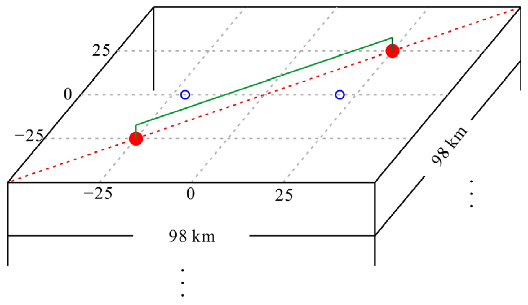
4.1. Homogenous Model

The size of the homogeneous half-space model is designed to be 98 km × 98 km × 98 km, with a resistivity of 100 Ω·m. Both the current entering and exiting the ground are 6250 A. The coordinates of the current exit and entry points, which are the positive and negative electrodes of the current source, are (0, −20, 0) km and (0, 20, 0) km, respectively. The coordinates of the grounding points at both ends of the conductor are (−25, 0, −25) km and (25, 0, 25) km. The positions of the current source and measurement points are shown in Figure 8.

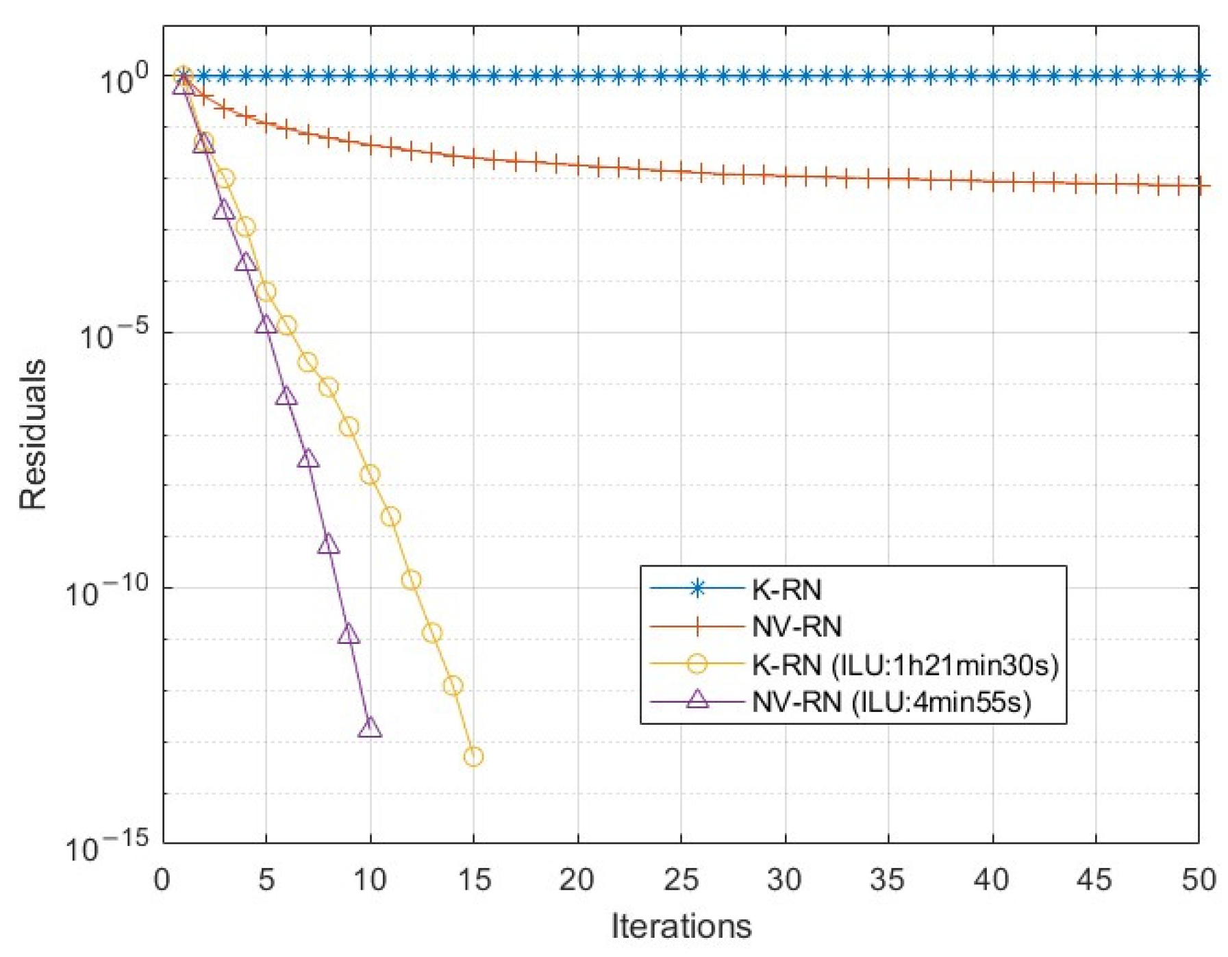
4.1.1. Comparison of Solving Efficiency

The system matrices generated via the two RN methods are shown in Figure 9. The system matrix generated via K-RN is mainly composed of two diagonal matrices combined, which correspond to the behavior of simulating the propagation process of current using the Kirchhoff current and voltage rules, respectively. The proposed NV-RN generates a symmetric diagonal system matrix without losing any unit information.
Using BiCGStab as the solver and ILU as the preconditioner [40,41], the solution processes of the two methods are compared, as shown in Figure 10. When the ILU preconditioner is not used, both K-RN and NV-RN are difficult to solve; the residuals of K-RN do not decrease, and the residuals of NV-RN decrease slowly with iterations. With the ILU preconditioner, the performance of the GMRES solver is significantly improved. Processing K-RN with ILU required 1 h, 21 min, and 30 s, while processing NV-RN required only 4 min and 55 s. This indicates that the diagonal system matrix generated via NV-RN is more favorable for solving.

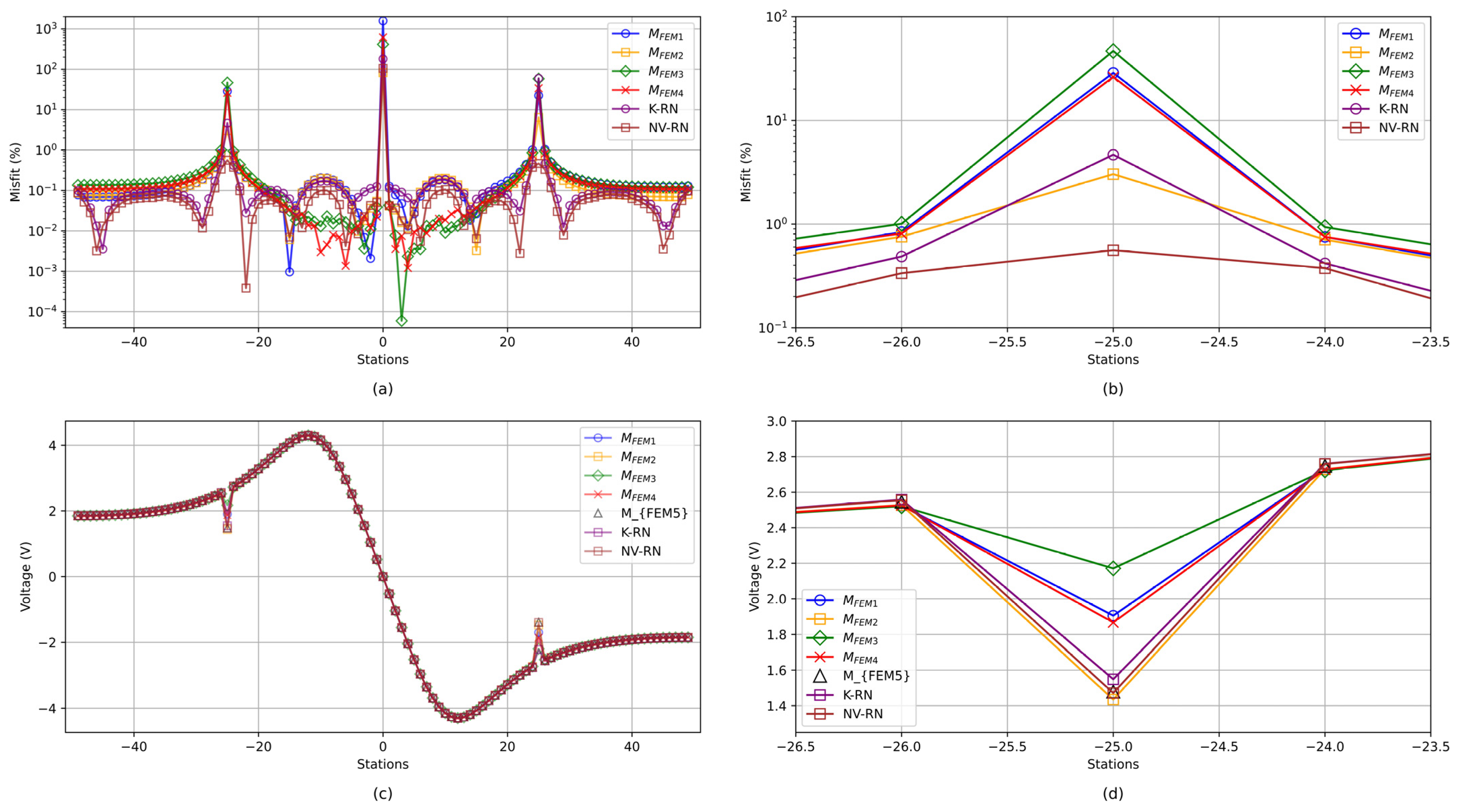
4.1.2. Mesh Discretization Efficiency

Two different mesh (Table 1) based finite element methods were used to compare the accuracy of the RN method. MFEM-1 and MFEM-2 use regular hexahedral grids, while MFEM-3, MFEM-4, and MFEM-5 use unstructured tetrahedral grids. Apart from the different grid types, these meshes also vary in density. Among them, MFEM-5 uses an adaptive algorithm based on a posteriori error estimates to generate the mesh used for calculating the standard response values [42].
MFEM-1 and MFEM-2 employ regular hexahedral grids to discretize the underground structure, with a lateral element length of 1 km. In both MFEM-1 and MFEM-2, the number of underground discretization elements is 0.97 × 10⁶. In MFEM-1, the number of mesh elements for discretizing the conductor is 10,598. In MFEM-2, the conductor is more densely discretized, resulting in 62,222 mesh elements. The total number of mesh elements in MFEM-1 and MFEM-2 are 0.98 × 10⁶ and 1.04 × 10⁶, respectively. MFEM-3 and MFEM-4 use unstructured tetrahedral grids with varying densities to discretize the underground structure. In MFEM-3, the total number of mesh elements is 0.06 × 10⁶, with 6996 elements for the conductor. In MFEM-4, the total number of mesh elements is 0.12 × 10⁶, with 61,191 elements for the conductor. MFEM-Bench represents the adaptive standard solution, where the underground structure is discretized using an unstructured tetrahedral grid and adaptive refinement at measurement points. The total number of mesh elements is 2.52 × 10⁶, with 117,481 elements for the conductor.
Comparing the solution results of K-RN and NV-RN, NV-RN achieved higher numerical accuracy with fewer elements (Figure 11). This is attributed to NV-RN’s strategy of constructing basic resistance network elements around the cell center. Unlike the K-RN method, NV-RN does not rely on the continuity of regular elements to establish an equipotential surface for a face’s circulating current. As a result, NV-RN can utilize MR grids or multi-level grids.

4.2. Abnormal Body Model

To verify the necessity of mesh refinement and the precision and effectiveness of MR mesh in 3D simulation, we consider the abnormal body model. We set the model symmetrically, as illustrated in the cross-sectional view of the main section at y = 0 m in Figure 12. The red cross denotes the point source with ±6250 A currents. The geological body has a surrounding resistivity of 100 Ω·m. The anomalous block area exhibits a distinct resistivity from the surrounding, measuring 1 Ω·m. The abnormal block’s dimensions are 11 km × 11 km × 5 km, with a burial depth of 1 km. SGs are regular hexahedral soil microelements of equal size, and the grid spacings are 90 m and 1000 m, denoted as SG1 and SG2, respectively. The MR grid is used to improve the grid resolution near the surface; the basic cell has an edge of 1000 m, and the fine grid spacing is 90 m, 200 m, and 330 m, labeled as MR1, MR2, and MR3, respectively.
The gray part in Figure 12 represents the grid refinement on the surface near the abnormal body. The number of grid elements of each CL is shown in Table 2. We take the FEM calculation results as the benchmark solution, calculate the relative error (%) distribution of the MR grid and SG forward results, and conduct logarithmic transformation.
As shown in Figure 13a, the forward error of SG2 above the anomalous body surface reaches 15% when the grid spacing is 1000 m, emphasizing the requirement for a finer grid in the target area. With the decrease in the grid spacing, the accuracy of the forward results above the anomalous body is improved by approximately 1.7%. However, the use of such a finely structured grid in the large area model increases the calculation time dramatically and places high demands on the CPU and memory.
The comparison of the forward results of MR3, MR2, and MR1 is represented in Figure 13a–d. With the decrease in the grid step size, the relative error of ESP gradually decreases. When the grid spacing of MR1 in the target area is reduced to 90 m, the forward accuracy above the anomalous body is less than 1.5%. Compared with SG1, MR1 ensures the accuracy of the target area and improves computational efficiency by 99.7%.

5. Conclusions

We propose a new MR grid-based RN forward calculation method. The purpose of this method is to improve the grid resolution of the RN method near the Earth’s surface to obtain higher computational efficiency and accuracy. In the implementation process, the MR grid is regarded as a space recursive grid. We addressed the equivalent resistance of three precisions at the hanging nodes and employed surfel interpolation to resolve the current exchange issue at the interface between the coarser and finer grids. The accuracy of the proposed algorithm was proven through comparisons with results from traditional structured grid-based computations in a typical layered-model scenario. On this basis, we used the MR grid to realize the efficient expansion of the electrical boundary. Compared with traditional proportional expansion, the computational efficiency of the MR grid was greatly improved under the premise of ensuring a calculation error of less than 1%. We showed through experiments that when there are abnormal bodies in the local superficial layer and the forward modeling accuracy is 1%, the calculation time of the proposed algorithm is reduced by 99.7% compared to that of the traditional RN. Given the practical necessity for higher accuracy in the surface potential at the substation junction, we employed the multi-resolution grid to improve the resolution in proximity to the substation and subsequently compared the results with FEM calculations. The experimental results show that compared with the traditional grid, the calculation results of the MR grid are closer to the real value.

Author Contributions

Conceptualization, R.L. and X.F.; methodology, L.D., R.L. and Y.D.; software, T.L.; validation, T.L. and T.H.; investigation, X.F.; data curation, R.L.; writing—original draft preparation, L.D., R.L. and Y.D.; visualization, X.F. and Y.D.; supervision, T.L.; project administration, R.L.; funding acquisition, T.H. All authors have read and agreed to the published version of the manuscript.

Funding

This research was funded by National Natural Science Foundation of China, grant numbers 42104072 and 52201363.

Data Availability Statement

Dataset available on request from the authors.

Conflicts of Interest

The authors declare no conflicts of interest.

References

  1. Li, R.; Yu, N.; Wang, E.; Sun, Z.; Wu, X.; Wang, X.; Ma, L. Airborne Transient Electromagnetic Simulation: Detecting Geoelectric Structures for HVdc Monopole Operation. IEEE Geosci. Remote Sens. Mag. 2022, 10, 274–288. [Google Scholar] [CrossRef]
  2. Yu, N.; Cai, Z.; Li, R.; Zhang, Q.; Gao, L.; Sun, Z. Calculation of Earth Surface Potential and Neutral Current Caused by HVDC Considering Three-Dimensional Complex Soil Structure. IEEE Trans. Electromagn. Compat. 2021, 63, 1480–1490. [Google Scholar] [CrossRef]
  3. Altaf, M.W.; Arif, M.T.; Islam, S.N.; Haque, M.E. Microgrid Protection Challenges and Mitigation Approaches–A Comprehensive Review. IEEE Access 2022, 10, 38895–38922. [Google Scholar] [CrossRef]
  4. Khalid, M.R.; Khan, I.A.; Hameed, S.; Asghar, M.S.J.; Ro, J.-S. A Comprehensive Review on Structural Topologies, Power Levels, Energy Storage Systems, and Standards for Electric Vehicle Charging Stations and Their Impacts on Grid. IEEE Access 2021, 9, 128069–128094. [Google Scholar] [CrossRef]
  5. Faúndez Urbina, C.A.; Alanís, D.C.; Ramírez, E.; Seguel, O.; Fustos, I.J.; Donoso, P.D.; de Miranda, J.H.; Rakonjac, N.; Palma, S.E.; Galleguillos, M. Estimating Soil Water Content in a Thorny Forest Ecosystem by Time-Lapse Electrical Resistivity Tomography (ERT) and HYDRUS 2D/3D Simulations. Hydrol. Process. 2023, 37, e15002. [Google Scholar] [CrossRef]
  6. Blechschmidt, J.; Ernst, O.G. Three Ways to Solve Partial Differential Equations with Neural Networks—A Review. GAMM-Mitteilungen 2021, 44, e202100006. [Google Scholar] [CrossRef]
  7. Bai, N.; Zhou, J.; Hu, X.; Han, B. 3D Edge-Based and Nodal Finite Element Modeling of Magnetotelluric in General Anisotropic Media. Comput. Geosci. 2022, 158, 104975. [Google Scholar] [CrossRef]
  8. Li, R.; Wang, J.; Kong, W.; Yu, N.; Li, T.; Wang, C. An Adaptive Hybrid Grids Finite-Element Approach for Plane Wave Three-Dimensional Electromagnetic Modeling. Comput. Geosci. 2023, 180, 105437. [Google Scholar] [CrossRef]
  9. Zhou, J.; Hu, X.; Xiao, T.; Cai, H.; Li, J.; Peng, R.; Long, Z. Three-Dimensional Edge-Based Finite Element Modeling of Magnetotelluric Data in Anisotropic Media with a Divergence Correction. J. Appl. Geophys. 2021, 189, 104324. [Google Scholar] [CrossRef]
  10. Pfeifer, N.; Kizilcay, M.; Malicki, P. Analytical and Numerical Study of an Iron-Core Shunt-Compensation Reactor on a Mixed Transmission Line. Electr. Power Syst. Res. 2023, 220, 109315. [Google Scholar] [CrossRef]
  11. Arshia, G. 3D Electrical Resistivity Forward Modeling Using the Kirchhoff’s Method for Solving an Equivalent Resistor Network. J. Appl. Geophys. 2018, 159, 135–145. [Google Scholar] [CrossRef]
  12. Yang, D.; Oldenburg, D.; Heagy, L. 3D DC Resistivity Modeling of Steel Casing for Reservoir Monitoring Using Equivalent Resistor Network. In Proceedings of the Seg Technical Program Expanded, Dallas, TX, USA, 16–21 October 2016. [Google Scholar]
  13. Zhang, D.; Li, J.; Hui, D. Coordinated Control for Voltage Regulation of Distribution Network Voltage Regulation by Distributed Energy Storage Systems. Prot. Control. Mod. Power Syst. 2018, 3, 3. [Google Scholar] [CrossRef]
  14. Asim, K.M.; Schorlemmer, D.; Hainzl, S.; Iturrieta, P.; Savran, W.H.; Bayona, J.A.; Werner, M.J. Multi-Resolution Grids in Earthquake Forecasting: The Quadtree Approach. Bull. Seismol. Soc. Am. 2023, 113, 333–347. [Google Scholar] [CrossRef]
  15. Müller, T.; Evans, A.; Schied, C.; Keller, A. Instant Neural Graphics Primitives with a Multiresolution Hash Encoding. ACM Trans. Graph. 2022, 41, 102:1–102:15. [Google Scholar] [CrossRef]
  16. Lowry, T.; Allen, M.; Shive, P. Singularity Removal—A Refinement of Resistivity Modeling Techniques. Geophysics 1989, 54, 766–774. [Google Scholar] [CrossRef]
  17. Zhang, Z.; Dan, Y.; Zou, J.; Liu, G.; Li, Y. Research on Discharging Current Distribution of Grounding Electrodes. IEEE Access 2019, 7, 59287–59298. [Google Scholar] [CrossRef]
  18. Zhu, L.; Jiang, H.; Yang, F.; Luo, H.; Li, W.; Han, J. FEM Analysis and Sensor-Based Measurement Scheme of Current Distribution for Grounding Electrode. Appl. Sci. 2020, 10, 8151. [Google Scholar] [CrossRef]
  19. Sun, J.; Zhang, D.; Sun, Z. A Finite Difference Method for Modeling the DC Electrical Potential Field Including Surface Topography. In SEG Technical Program Expanded Abstracts 2009; SEG Technical Program Expanded Abstracts; Society of Exploration Geophysicists: Houston, TX, USA, 2009; pp. 664–668. [Google Scholar]
  20. Pidlisecky, A.; Haber, E.; Knight, R. RESINVM3D: A 3D Resistivity Inversion Package. Geophysics 2007, 72, H1–H10. [Google Scholar] [CrossRef]
  21. Hetita, I.; Zalhaf, A.S.; Mansour, D.-E.A.; Han, Y.; Yang, P.; Wang, C. Modeling and Protection of Photovoltaic Systems during Lightning Strikes: A Review. Renew. Energy 2022, 184, 134–148. [Google Scholar] [CrossRef]
  22. Kim, Y.W.; Oh, I.H.; Choi, S.; Nam, I.; Chang, S.T. Vertical Integration of Multi-Electrodes inside a Single Sheet of Paper and the Control of the Equivalent Circuit for High-Density Flexible Supercapacitors. Chem. Eng. J. 2023, 454, 140117. [Google Scholar] [CrossRef]
  23. Molero, C.; Alex-Amor, A.; Mesa, F.; Palomares-Caballero, Á.; Padilla, P. Cross-Polarization Control in FSSs by Means of an Equivalent Circuit Approach. IEEE Access 2021, 9, 99513–99525. [Google Scholar] [CrossRef]
  24. Hussain, S.M.; Jamshed, W. A Comparative Entropy Based Analysis of Tangent Hyperbolic Hybrid Nanofluid Flow: Implementing Finite Difference Method. Int. Commun. Heat Mass Transf. 2021, 129, 105671. [Google Scholar] [CrossRef]
  25. Rasheed, M.; Ali, A.H.; Alabdali, O.; Shihab, S.; Rashid, A.; Rashid, T.; Hamad, S.H.A. The Effectiveness of the Finite Differences Method on Physical and Medical Images Based on a Heat Diffusion Equation. J. Phys. Conf. Ser. 2021, 1999, 012080. [Google Scholar] [CrossRef]
  26. Cai, H.; Liu, M.; Zhou, J.; Li, J.; Hu, X. Effective 3D-Transient Electromagnetic Inversion Using Finite-Element Method with a Parallel Direct Solver. Geophysics 2022, 87, E377–E392. [Google Scholar] [CrossRef]
  27. Long, Z.; Cai, H.; Hu, X.; Zhou, J.; Yang, X. Three-Dimensional Inversion of CSEM Data Using Finite Element Method in Data Space. IEEE Trans. Geosci. Remote Sens. 2024, 62, 2001711. [Google Scholar] [CrossRef]
  28. Yao, H.; Ren, Z.; Tang, J.; Lin, Y.; Yin, C.; Hu, X.; Huang, Q.; Zhang, K. 3D Finite-Element Modeling of Earth Induced Electromagnetic Field and Its Potential Applications for Geomagnetic Satellites. Sci. China Earth Sci. 2021, 64, 1798–1812. [Google Scholar] [CrossRef]
  29. Cai, H.; Kong, R.; He, Z.; Wang, X.; Liu, S.; Huang, S.; Kass, M.A.; Hu, X. Joint Inversion of Potential Field Data with Adaptive Unstructured Tetrahedral Mesh. Geophysics 2024, 89, G45–G63. [Google Scholar] [CrossRef]
  30. Han, X.; Yin, C.; Su, Y.; Zhang, B.; Liu, Y.; Ren, X.; Ni, J.; Farquharson, C.G. 3D Finite-Element Forward Modeling of Airborne EM Systems in Frequency-Domain Using Octree Meshes. IEEE Trans. Geosci. Remote Sens. 2022, 60, 5912813. [Google Scholar] [CrossRef]
  31. Liu, Y.; Yogeshwar, P.; Peng, R.; Hu, X.; Han, B.; Blanco-Arrué, B. Three-Dimensional Inversion of Time-Domain Electromagnetic Data Using Various Loop Source Configurations. IEEE Trans. Geosci. Remote Sens. 2024, 62, 5910515. [Google Scholar] [CrossRef]
  32. Peng, R.; Han, B.; Liu, Y.; Hu, X. EM3DANI: A Julia Package for Fully Anisotropic 3D Forward Modeling of Electromagnetic Data. Geophysics 2021, 86, F49–F60. [Google Scholar] [CrossRef]
  33. Yang, H.; Cai, H.; Liu, M.; Xiong, Y.; Long, Z.; Li, J.; Hu, X. Three-dimensional Inversion of Semi-airborne Transient Electromagnetic Data Based on Finite Element Method. Near Surf. Geophys. 2022, 20, 661–678. [Google Scholar] [CrossRef]
  34. Zhou, J.; Bai, N.; Hu, X.; Xiao, T. An Efficient Hybrid Direct-Iterative Solver for Three-Dimensional Higher-Order Edge-Based Finite Element Simulation for Magnetotelluric Data in Anisotropic Media. Phys. Earth Planet. Inter. 2023, 339, 107029. [Google Scholar] [CrossRef]
  35. Gillis, T.; van Rees, W.M. MURPHY---A Scalable Multiresolution Framework for Scientific Computing on 3D Block-Structured Collocated Grids. SIAM J. Sci. Comput. 2022, 44, C367–C398. [Google Scholar] [CrossRef]
  36. Xie, J.; Cai, H.; Hu, X.; Long, Z.; Xu, S.; Fu, C.; Wang, Z.; Di, Q. 3-D Magnetotelluric Inversion and Application Using the Edge-Based Finite Element with Hexahedral Mesh. IEEE Trans. Geosci. Remote Sens. 2022, 60, 4503011. [Google Scholar] [CrossRef]
  37. Tang, W.; Li, Y.; Liu, J.; Deng, J. Three-Dimensional Controlled-Source Electromagnetic Forward Modeling by Edge-Based Finite Element with a Divergence Correction. Geophysics 2021, 86, E367–E382. [Google Scholar] [CrossRef]
  38. Haber, E.; Heldmann, S.; Modersitzki, J. An Octree Method for Parametric Image Registration. SIAM J. Sci. Comput. 2007, 29, 2008–2023. [Google Scholar] [CrossRef]
  39. Horesh, L.; Haber, E. A Second Order Discretization of Maxwell’s Equations in the Quasi-Static Regime on Octree Grids. SIAM J. Sci. Comput. 2011, 33, 2805–2822. [Google Scholar] [CrossRef]
  40. Saad, Y.; Schultz, M.H. GMRES: A Generalized Minimal Residual Algorithm for Solving Nonsymmetric Linear Systems. SIAM J. Sci. Stat. Comput. 1986, 7, 856–869. [Google Scholar] [CrossRef]
  41. Calgaro, C.; Chehab, J.-P.; Saad, Y. Incremental Incomplete LU Factorizations with Applications. Numer. Linear Algebra Appl. 2010, 17, 811–837. [Google Scholar] [CrossRef]
  42. Ren, Z.; Qiu, L.; Tang, J.; Wu, X.; Xiao, X.; Zhou, Z. 3-D Direct Current Resistivity Anisotropic Modelling by Goal-Oriented Adaptive Finite Element Methods. Oxf. Acad. 2018, 212, 76–87. [Google Scholar] [CrossRef]
Figure 1. The flow direction of current in the ground DC return system during monopole operation.
Mathematics 12 02392 g001
Figure 2. Discrete schematic diagram of three-dimensional field-circuit coupling model.
Mathematics 12 02392 g002
Figure 3. MR grid structure. The left area represents unrefined units, while the right block is subdivided into eight parts. The refinement levels are denoted by coarseness level (CL), where the unrefined cell spacing is 10, and the refined cell spacing is 5. This grid can be described as [CL, Sp] = [1, 5; 2, 10]. The red part represents the interface where the hanging node is located.
Mathematics 12 02392 g003
Figure 4. Hanging nodes. Hanging surfaces and interpolation methods. (a) Hanging nodes. (b) Hanging surfaces and interpolation methods. The serial number represents the index of the hanging node.
Mathematics 12 02392 g004
Figure 5. Discretization of the gradient. (a) Case CS: calculation is based on hc. (b) Case FS: calculation is based on hf. (c) Case GF: second-order discretization of gradient.
Mathematics 12 02392 g005
Figure 6. Three-dimensional multi-resolution grid RN. (a) Case CS and GF. (b) Case FS.
Mathematics 12 02392 g006
Figure 7. The boundary resistance setting at the unit center calculation model.
Mathematics 12 02392 g007
Figure 8. Schematic diagram of a homogeneous half-space model. The blue circle represents the position of the current source. The green line represents a long-distance straight wire, and the red dot represents the grounding electrode of the wire. The red dashed line represents the measurement line for observing the response signal.
Mathematics 12 02392 g008
Figure 9. Distribution of main elements in the system matrix generated via K-RN and NV-RN. (a) Represents the distribution of the main elements in the system matrix of K-RN, and (b) represents the distribution of the main elements in the system matrix of NV-RN.
Mathematics 12 02392 g009
Figure 10. Reduction of residuals with number of iteration steps during the KRN and NV-RN solution.
Mathematics 12 02392 g010
Figure 11. Calculation results of RN and FEM for numerical simulation of terrestrial reflux. (a) Represents the voltage response result on the measuring line, (b) represents the voltage response error on the measuring line, (c) represents the voltage response result at the grounding electrode, and (d) represents the voltage response error at the grounding electrode.
Mathematics 12 02392 g011
Figure 12. 3-D anomaly body model main section (y = 0 m) and the discretization on a multi-resolution grid.
Mathematics 12 02392 g012
Figure 13. Comparison of ESP (z = 0 m) relative errors (%) of different meshing strategies for the 3D anomaly body model (log10 transformation) with the FEM results. (a) SG2. (b) MR3. (c) MR2. (d) MR1. (e) SG1 approach.
Mathematics 12 02392 g013
Table 1. Mesh generation of RN and FEM.
NV-RNKRNMFEM-1MFEM-2MFEM-3MFEM-4MFEM-Bench
Mesh TypeHexahedronTetrahedron
Ground NoE (1.0 × 10⁶)0.984.30.970.970.050.062.4
Line NoE 10,59862,222699661,191117,481
Total NoE (1.0 × 10⁶)0.984.30.981.040.060.122.52
Run time (s)23127666125364084633,744
Table 2. Grid subdivision strategies and solution efficiency for the 3D anomalous body model.
Grid TypeRange
(X, km)
Depth
(Z, m)
CLGrid Spacing
(km)
Grid NumberDoFsSolving
IterTime
MR1−20.5–20.50–710.0915661877158164854423 min 56 s
−27.5–27.57–5521154608
MR2−20.5–20.50–710.21470875162548335431 s
−27.5–27.57–5521154608
MR3−20.5–20.50–710.3331770947231726114 s
−27.5–27.57–5521154608
SG1−27.5–27.50–7 0.09221445125221445125165420 h 3 min 29 s
SG2−27.5–27.57–55111663751663751843.02 s
Disclaimer/Publisher’s Note: The statements, opinions and data contained in all publications are solely those of the individual author(s) and contributor(s) and not of MDPI and/or the editor(s). MDPI and/or the editor(s) disclaim responsibility for any injury to people or property resulting from any ideas, methods, instructions or products referred to in the content.

