
Stochastic Multi-Objective Multi-Trip AMR Routing Problem with Time Windows


Abstract
1. Introduction
- Formulate the SMMAMRRPTW and establish a stochastic programming model.;
- Develop a population-based tabu search algorithm (PTS);
- Demonstrate the effectiveness and robustness of the PTS algorithm through numerical experiments, compared with other algorithms, and provide relevant management insights.
2. Literature Review
3. Problem Description and Formulation
3.1. Problem Description
3.2. Model Formulation
4. Proposed Population-Based Tabu Search Algorithm
| Algorithm 1 Population-based tabu search (PTS) algorithm |
| Input: , , , . |
Output:
|
4.1. Evaluation of Solution
4.2. Initial Solution
| Algorithm 2 Gk algorithm |
| Input: , |
Output: solution
|
4.3. Tabu Search
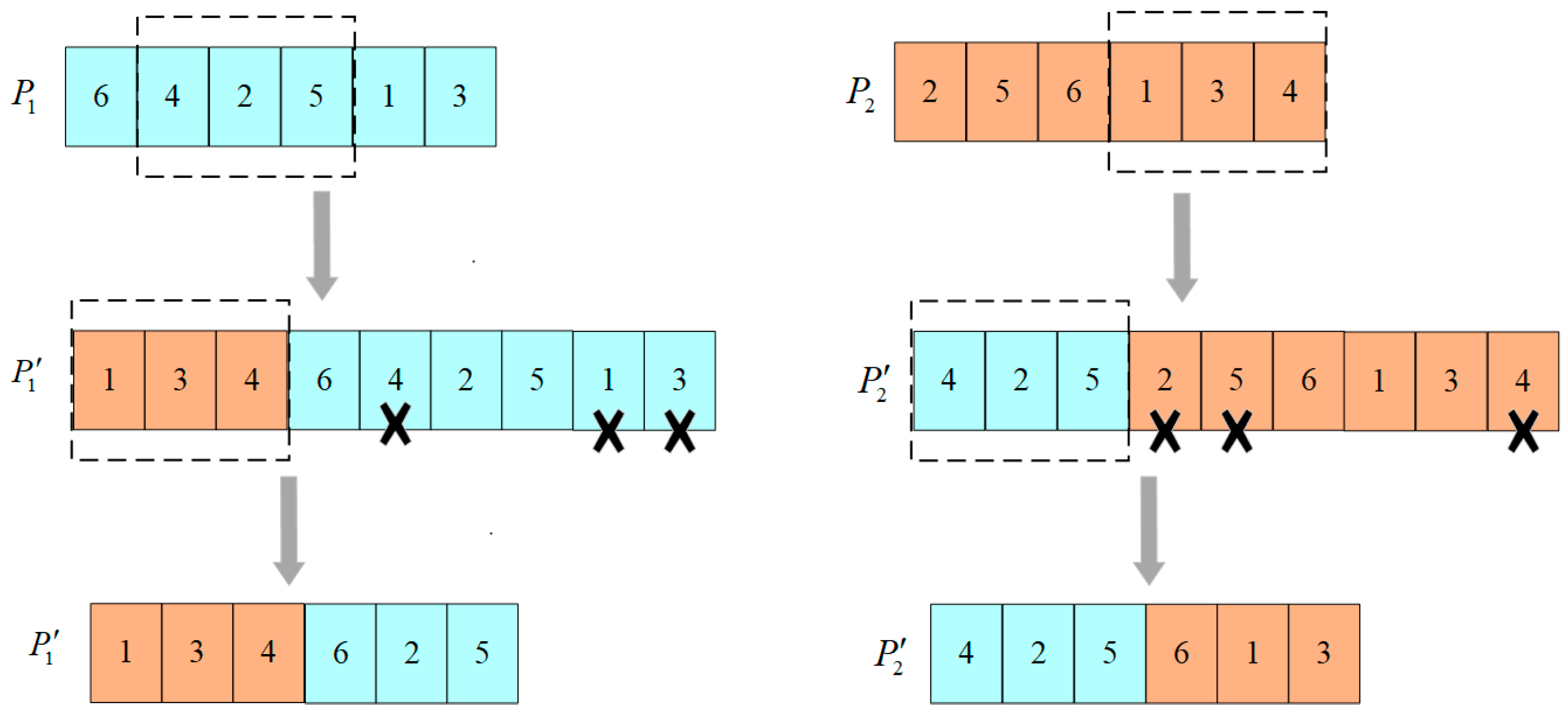
4.4. Crossover Operators
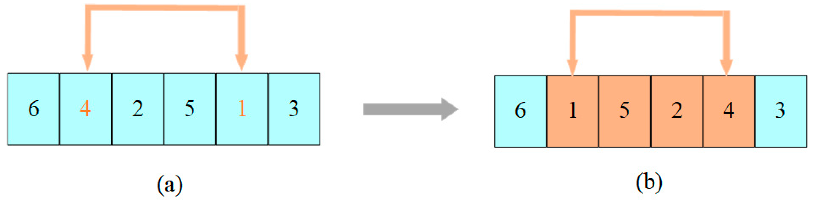
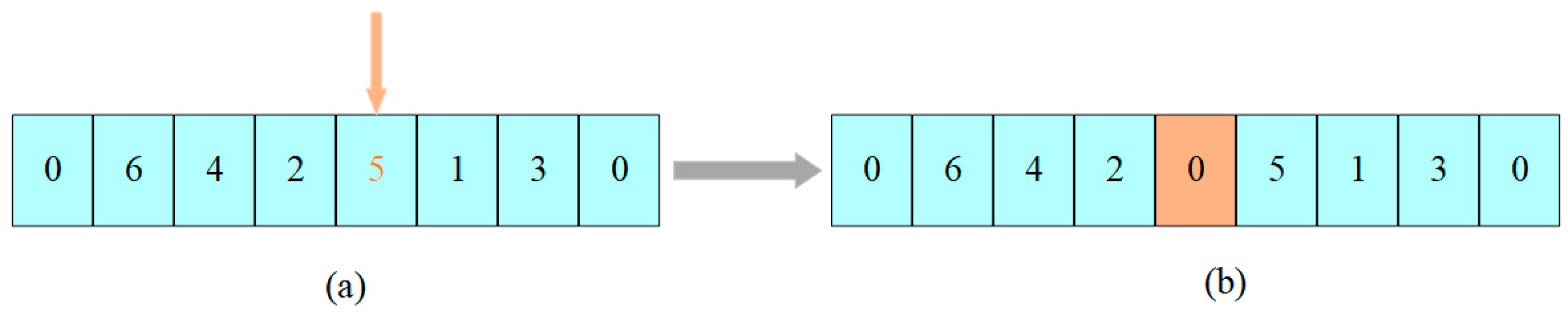
4.5. Mutation Operators
4.6. PTS Algorithm Stop Condition
5. Computational Study
5.1. Dataset Generation
5.2. Parameter Setting
5.3. Performance of the PTS Algorithm

| Instance | Gk | k-Means | Greedy Insertion | ||||
|---|---|---|---|---|---|---|---|
| C101 | 2,045,910.08 | 1,863,415 | 2,610,782 | 2,417,649 | 21.63 | 2,617,170 | 21.82 |
| C102 | 1,254,631.38 | 1,107,483 | 1,655,803 | 1,434,495 | 24.22 | 1,870,543 | 32.92 |
| C201 | 12,085,514.7 | 8,324,882 | 14,809,985 | 11,851,861 | 18.39 | 7,814,317 | −54.65 |
| C202 | 9,612,167.96 | 8,365,007 | 12,044,963 | 9,850,724 | 20.19 | 9,311,346 | −3.23 |
| R101 | 938,552.54 | 884,402.9 | 959,881.3 | 830,621 | 2.22 | 1,166,671 | 19.55 |
| R102 | 742,706.32 | 686,893 | 797,058 | 739,009.9 | 6.81 | 953,384.5 | 22.09 |
| R201 | 5,093,775.34 | 3,129,344 | 7,378,546 | 6,652,661 | 30.96 | 5,823,723 | 12.53 |
| R202 | 4,614,830.48 | 2,115,929 | 6,124,538 | 5,632,099 | 24.65 | 6,014,803 | 23.27 |
| RC101 | 830,637.94 | 718,604 | 785,494.6 | 734,688.3 | −5.74 | 1,015,725 | 18.22 |
| RC102 | 693,004.58 | 628,846.4 | 666,737.6 | 576,412 | −3.93 | 929,352.6 | 25.43 |
| RC201 | 4,923,085.68 | 3,848,542 | 591,6827 | 5,416,624 | 16.79 | 5,317,144 | 7.41 |
| RC202 | 3,916,137.13 | 2,559,224 | 5,231,515 | 4,386,069 | 25.14 | 5,463,542 | 28.32 |
| Average | 3,895,912.85 | 2,852,714.40 | 4,915,177.43 | 4,210,242.97 | 20.73 | 4,024,810.2 | 3.20 |
| Instance | TS | GA | PTS | ||||||||
|---|---|---|---|---|---|---|---|---|---|---|---|
| CPU (s) | CPU (s) | CPU (s) | |||||||||
| C101 | 1,018,859 | 1,122,640 | 41.68 | 1,339,227 | 1,465,171 | 20.41 | 794,186.5 | 934,713.9 | 70.44 | 20.1 | 56.7 |
| C102 | 544,306.6 | 660,273.5 | 40.60 | 850,956.7 | 887,624.5 | 20.36 | 383,453.1 | 510,149.9 | 89.07 | 29.4 | 74.0 |
| C201 | 5,875,695 | 6,200,411 | 36.04 | 6,794,412 | 7,638,171 | 14.80 | 5,300,789 | 5,857,005 | 80.19 | 5.9 | 30.4 |
| C202 | 2,707,980 | 4,023,706 | 43.43 | 3,946,166 | 4,838,110 | 16.86 | 3,032,538 | 3,568,176 | 77.69 | 12.8 | 35.6 |
| R101 | 601,024.8 | 630,914.4 | 44.75 | 777,221.5 | 805,799.9 | 18.74 | 564,001.8 | 615,274.9 | 81.56 | 2.54 | 31.0 |
| R102 | 462,079 | 496,479.4 | 41.56 | 605,469.9 | 639,811.3 | 20.42 | 428,810.9 | 459,041.6 | 70.80 | 8.16 | 39.4 |
| R201 | 2,041,798 | 2,366,187 | 42.13 | 2,624,790 | 2,975,805 | 16.96 | 1,886,346 | 2,267,428 | 68.81 | 4.36 | 31.2 |
| R202 | 1,626,803 | 1,862,737 | 38.31 | 1,915,175 | 2,140,760 | 16.53 | 1,518,544 | 1,679,639 | 71.34 | 10.9 | 27.5 |
| RC101 | 535,131.9 | 572,251 | 48.61 | 652,803.2 | 709,288.6 | 20.72 | 484,415.7 | 548,133.4 | 72.90 | 4.4 | 29.4 |
| RC102 | 445,098.8 | 480,440.4 | 47.07 | 567,694.6 | 587,258.1 | 19.31 | 415,750.2 | 443,555.7 | 72.34 | 8.32 | 32.4 |
| RC201 | 1,888,989 | 2,147,014 | 43.4 | 2,682,160 | 2,991,024 | 17.10 | 1,689,098 | 2,106,756 | 72.36 | 1.91 | 42.0 |
| RC202 | 1,505,167 | 1,707,251 | 44.33 | 1,775,964 | 2,111,596 | 17.25 | 1,275,220 | 1,499,864 | 70.56 | 13.8 | 40.8 |
| Average | 1,604,411 | 1,855,859 | 42.66 | 2,044,337 | 2,315,868 | 18.29 | 1,481,096 | 1,707,478 | 74.84 | 8.69 | 35.6 |
5.4. Sensitivity Analysis and Management Insights
6. Conclusions
Author Contributions
Funding
Data Availability Statement
Conflicts of Interest
References
- Chen, L.-K. Advancing the journey: Taiwan’s ongoing efforts in reshaping the future for aging populations. Arch. Gerontol. Geriatr. 2023, 113, 105128. [Google Scholar] [CrossRef] [PubMed]
- Dijkman, B.L.; Hirjaba, M.; Wang, W.; Palovaara, M.; Annen, M.; Varik, M.; Cui, Y.a.; Li, J.; van Slochteren, C.; Jihong, W.; et al. Developing a competence framework for gerontological nursing in China: A two-phase research design including a needs analysis and verification study. BMC Nurs. 2022, 21, 285. [Google Scholar] [CrossRef] [PubMed]
- Sommer, D.; Kasbauer, J.; Jakob, D.; Schmidt, S.; Wahl, F. Potential of assistive robots in clinical nursing: An observational study of nurses’ transportation tasks in rural clinics of bavaria, germany. Nurs. Rep. 2024, 14, 267–286. [Google Scholar] [CrossRef] [PubMed]
- Ozturkcan, S.; Merdin-Uygur, E. Humanoid service robots: The future of healthcare? J. Inf. Technol. Teach. Cases 2021, 12, 163–169. [Google Scholar] [CrossRef]
- Ding, N.; Peng, C.; Lin, M.; Wu, C. A comprehensive review on automatic mobile robots: Applications, perception, communication and control. J. Circuits Syst. Comput. 2022, 31, 2250153. [Google Scholar] [CrossRef]
- Zou, W.; Zou, J.; Sang, H.; Meng, L.; Pan, Q. An effective population-based iterated greedy algorithm for solving the multi-AGV scheduling problem with unloading safety detection. Inf. Sci. 2024, 657, 119949. [Google Scholar] [CrossRef]
- Zhang, X.-J.; Sang, H.-Y.; Li, J.-Q.; Han, Y.-Y.; Duan, P. An effective multi-AGVs dispatching method applied to matrix manufacturing workshop. Comput. Ind. Eng. 2022, 163, 107791. [Google Scholar] [CrossRef]
- Zou, W.-Q.; Pan, Q.-K.; Meng, L.-L.; Sang, H.-Y.; Han, Y.-Y.; Li, J.-Q. An effective self-adaptive iterated greedy algorithm for a multi-AGVs scheduling problem with charging and maintenance. Expert Syst. Appl. 2023, 216, 119512. [Google Scholar] [CrossRef]
- Aziez, I.; Côté, J.-F.; Coelho, L.C. Fleet sizing and routing of healthcare automated guided vehicles. Transport. Res. Part E Logist. Transp. Rev. 2022, 161, 102679. [Google Scholar] [CrossRef]
- Cheng, L.; Zhao, N.; Wu, K.; Chen, Z. The multi-trip autonomous mobile robot scheduling problem with time windows in a stochastic environment at smart hospitals. Appl. Sci. 2023, 13, 9879. [Google Scholar] [CrossRef]
- Nishi, T.; Hiranaka, Y.; Grossmann, I.E. A bilevel decomposition algorithm for simultaneous production scheduling and conflict-free routing for automated guided vehicles. Comput. Oper. Res. 2011, 38, 876–888. [Google Scholar] [CrossRef]
- Chikul, M.; Maw, H.Y.; Soong, Y.K. Technology in healthcare: A case study of healthcare supply chain management models in a general hospital in Singapore. J. Hosp. Adm. 2017, 6, 63–70. [Google Scholar] [CrossRef]
- Zou, W.-Q.; Pan, Q.-K.; Meng, T.; Gao, L.; Wang, Y.-L. An effective discrete artificial bee colony algorithm for multi-AGVs dispatching problem in a matrix manufacturing workshop. Expert Syst. Appl. 2020, 161, 113675. [Google Scholar] [CrossRef]
- Han, W.-J.; Xu, J.; Sun, Z.; Liu, B.; Zhang, K.; Zhang, Z.-H.; Mei, X.-S. Digital twin-based automated guided vehicle scheduling: A solution for its charging problems. Appl. Sci. 2022, 12, 3354. [Google Scholar] [CrossRef]
- Cheng, L.; Zhao, N.; Yuan, M.; Wu, K. Stochastic scheduling of autonomous mobile robots at hospitals. PLoS ONE 2023, 18, e0292002. [Google Scholar] [CrossRef] [PubMed]
- Gendreau, M.; Guertin, F.; Potvin, J.Y.; Seguin, R. Neighborhood search heuristics for a dynamic vehicle dispatching problem with pick-ups and deliveries. Transp. Res. Part C Emerg. Technol. 2006, 14, 157–174. [Google Scholar] [CrossRef]
- Biesinger, B.; Hu, B.; Raidl, G.R. A genetic algorithm in combination with a solution archive for solving the generalized vehicle routing problem with stochastic demands. Transport. Sci. 2018, 52, 673–690. [Google Scholar] [CrossRef]
- Goel, R.; Maini, R.; Bansal, S. Vehicle routing problem with time windows having stochastic customers demands and stochastic service times: Modelling and solution. J. Comput. Sci. 2019, 34, 1–10. [Google Scholar] [CrossRef]
- Çimen, M.; Soysal, M. Time-dependent green vehicle routing problem with stochastic vehicle speeds: An approximate dynamic programming algorithm. Transp. Res. Part D Transp. Environ. 2017, 54, 82–98. [Google Scholar] [CrossRef]
- Elgharably, N.; Easa, S.; Nassef, A.; Damatty, A.E. Stochastic multi-objective vehicle routing model in green environment with customer satisfaction. IEEE Trans. Intell. Transp. Syst. 2023, 24, 1337–1355. [Google Scholar] [CrossRef]
- Xie, F.; Chen, Z.; Zhang, Z. Research on dynamic takeout delivery vehicle routing problem under time-varying subdivision road network. Mathematics 2024, 12, 962. [Google Scholar] [CrossRef]
- Lenstra, J.K.; Kan, A.H.G.R. Complexity of vehicle routing and scheduling problems. Networks 1981, 11, 221–227. [Google Scholar] [CrossRef]
- Braekers, K.; Ramaekers, K.; Van Nieuwenhuyse, I. The vehicle routing problem: State of the art classification and review. Comput. Ind. Eng. 2016, 99, 300–313. [Google Scholar] [CrossRef]
- Li, G.; Li, J. An improved tabu search algorithm for the stochastic vehicle routing problem with soft time windows. IEEE Access 2020, 8, 158115–158124. [Google Scholar] [CrossRef]
- Wu, Y.; Du, H.; Song, H. An iterated local search heuristic for the multi-trip vehicle routing problem with multiple time windows. Mathematics 2024, 12, 1712. [Google Scholar] [CrossRef]
- Hashemi-Amiri, O.; Mohammadi, M.; Rahmanifar, G.; Hajiaghaei-Keshteli, M.; Fusco, G.; Colombaroni, C. An allocation-routing optimization model for integrated solid waste management. Expert Syst. Appl. 2023, 227, 120364. [Google Scholar] [CrossRef]
- Tan, K.C.; Cheong, C.Y.; Goh, C.K. Solving multiobjective vehicle routing problem with stochastic demand via evolutionary computation. Eur. J. Oper. Res. 2007, 177, 813–839. [Google Scholar] [CrossRef]
- Ehmke, J.F.; Campbell, A.M.; Urban, T.L. Ensuring service levels in routing problems with time windows and stochastic travel times. Eur. J. Oper. Res. 2015, 240, 539–550. [Google Scholar] [CrossRef]
- Nadarajah, S.; Kotz, S. Exact distribution of the max/min of two gaussian random variables. IEEE Trans. Very Large Scale Integr. (VLSI) Syst. 2008, 16, 210–212. [Google Scholar] [CrossRef]
- Glover, F. Future paths for integer programming and links to artificial intelligence. Comput. Oper. Res. 1986, 13, 533–549. [Google Scholar] [CrossRef]
- Vidal, T.; Crainic, T.G.; Gendreau, M.; Prins, C. A hybrid genetic algorithm with adaptive diversity management for a large class of vehicle routing problems with time-windows. Comput. Oper. Res. 2013, 40, 475–489. [Google Scholar] [CrossRef]
- Huang, H.; Hu, C.; Zhu, J.; Wu, M.; Malekian, R. Stochastic task scheduling in UAV-based intelligent on-demand meal delivery system. IEEE Trans. Intell. Transp. Syst. 2022, 23, 13040–13054. [Google Scholar] [CrossRef]
- Wang, Q.; Li, H.; Wang, D.; Cheng, T.C.E.; Yin, Y. Bi-objective perishable product delivery routing problem with stochastic demand. Comput. Ind. Eng. 2023, 175, 108837. [Google Scholar] [CrossRef]
- Chen, B.; Zeng, W.; Lin, Y.; Zhang, D. A new local search-based multiobjective optimization algorithm. IEEE Trans. Evol. Comput. 2015, 19, 50–73. [Google Scholar] [CrossRef]
- Zandieh, M.; Moradi, H. An imperialist competitive algorithm in mixed-model assembly line sequencing problem to minimise unfinished works. Int. J. Syst. Sci. Oper. Logist. 2019, 6, 179–192. [Google Scholar] [CrossRef]


| Sets | |
| Set of requests | |
| Set of the route traveled by the AMR | |
| Parameters | |
| Cargo capacity of the AMR | |
| Fixed cost of the AMR | |
| Cost per unit time | |
| Demand of request | |
| Service time of request | |
| Waiting time of the AMR at the request on the route | |
| Travel time spent by the AMR on the route from request to request | |
| Remaining capacity of the AMR when it arrives at request on its route | |
| Time when the AMR arrives at the request on the route | |
| Start service request time of the AMR on the route | |
| Time window of request | |
| Decision variables | |
| 1 if the AMR completes request and successively on its route; 0 otherwise | |
| Number of AMRs participating in medical request services | |
| 1 if the AMR completes service request on its route; 0 otherwise | |
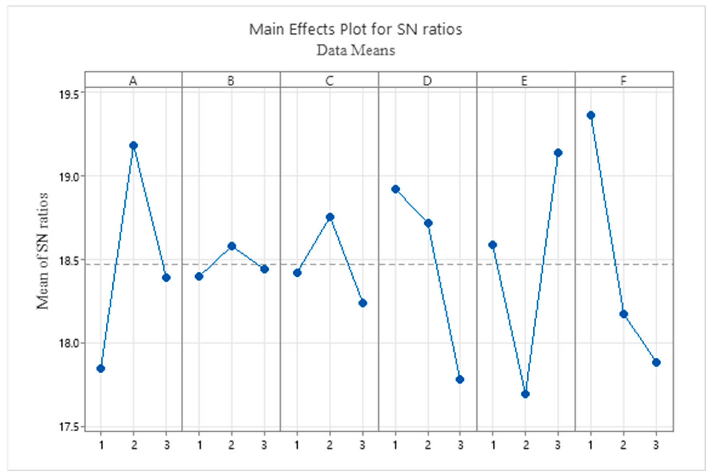
| Parameters | Factors | Parameter Levels | Optimum Level | ||
|---|---|---|---|---|---|
| Level 1 | Level 2 | Level 3 | |||
| k-means iter | A | 20 | 30 | 40 | 30 |
| k-means threshold | B | 0.0001 | 0.0002 | 0.0003 | 0.0002 |
| Population size | C | 100 | 120 | 150 | 120 |
| Probability crossover | D | 0.7 | 0.8 | 0.9 | 0.7 |
| Probability mutation | E | 0.05 | 0.1 | 0.15 | 0.15 |
| Maximum number of iterations PTS | F | 50 | 200 | 500 | 50 |
Disclaimer/Publisher’s Note: The statements, opinions and data contained in all publications are solely those of the individual author(s) and contributor(s) and not of MDPI and/or the editor(s). MDPI and/or the editor(s) disclaim responsibility for any injury to people or property resulting from any ideas, methods, instructions or products referred to in the content. |
© 2024 by the authors. Licensee MDPI, Basel, Switzerland. This article is an open access article distributed under the terms and conditions of the Creative Commons Attribution (CC BY) license (https://creativecommons.org/licenses/by/4.0/).
Share and Cite
Cheng, L.; Zhao, N.; Wu, K. Stochastic Multi-Objective Multi-Trip AMR Routing Problem with Time Windows. Mathematics 2024, 12, 2394. https://doi.org/10.3390/math12152394
Cheng L, Zhao N, Wu K. Stochastic Multi-Objective Multi-Trip AMR Routing Problem with Time Windows. Mathematics. 2024; 12(15):2394. https://doi.org/10.3390/math12152394
Chicago/Turabian StyleCheng, Lulu, Ning Zhao, and Kan Wu. 2024. "Stochastic Multi-Objective Multi-Trip AMR Routing Problem with Time Windows" Mathematics 12, no. 15: 2394. https://doi.org/10.3390/math12152394
APA StyleCheng, L., Zhao, N., & Wu, K. (2024). Stochastic Multi-Objective Multi-Trip AMR Routing Problem with Time Windows. Mathematics, 12(15), 2394. https://doi.org/10.3390/math12152394