Optimizing the Capacity Allocation of the Chinese Hierarchical Healthcare System under Heavy Traffic Conditions

Abstract

In this study, we explore optimal service allocation within the Chinese hierarchical healthcare system with green channels, providing valuable insights for practitioners to understand how optimal service allocation is affected by various realistic factors. These green channels are designed to streamline referrals from community healthcare centers to comprehensive hospitals. We aim to determine the optimal capacity allocation for these green channels within comprehensive hospitals. Our research employs techniques from queuing theory and stochastic processes, e.g., diffusion analysis, to develop a mathematical model that approximates the optimal allocation of resources. We uncover both closed-form and numerical solutions for this optimal capacity allocation. By analyzing the impact of various cost factors, we find that an increase in costs within the green channel results in a lower optimal service rate. Additionally, patient preferences for specific treatments influence allocation, reducing the optimal share of services provided by general hospitals. The optimal solution is also affected by the proportions of different patient types. Through extensive simulations, we validate the accuracy of our model approximations under heavy traffic conditions, further examining sources of error to ensure robustness. Our findings provide valuable insights into optimizing resource allocation in hierarchical healthcare systems, ensuring efficient and cost-effective patient care.

1. Introduction

In recent years, the gatekeeper service mechanism has been increasingly applied in foreign healthcare systems. In foreign gatekeeper service systems, patients are initially assessed by gatekeepers. If the gatekeepers cannot resolve the issue, the patients are referred to specialists for final care, as shown in Figure 1a. This service mechanism significantly reduces service costs and improves efficiency.

In China, a similar gatekeeper system, known as the Chinese hierarchical healthcare system, is also in place, as shown in Figure 1b. The Chinese hierarchical healthcare system is designed to streamline patient care and optimize resource utilization by categorizing medical institutions into two main types: community health centers and comprehensive hospitals. Comprehensive hospitals are equipped with more advanced medical facilities and specialized doctors, resulting in higher medical standards. These hospitals handle complex cases that require specialized medical expertise and sophisticated treatment methods. They serve as the upper tier in the healthcare hierarchy, providing secondary and tertiary care. On the other hand, community health centers form the primary tier of the healthcare system. These centers have limited equipment and mostly employ general practitioners, leading to lower medical service capabilities. They are designed to handle routine and less severe medical conditions, such as common colds, minor injuries, and chronic disease management. If the condition is beyond the capacity of these centers, patients are referred to comprehensive hospitals [1]. This referral system is intended to reduce the burden on comprehensive hospitals, prevent overcrowding, and make efficient use of healthcare resources.

However, the implementation of the hierarchical diagnosis and treatment system has encountered several challenges. One of the primary challenges is the need for optimal capacity allocation and process optimization within comprehensive hospitals to ensure seamless patient flow and cost-effective operations. To address these issues, the Beijing municipal government has introduced a hierarchical medical system with a green channel, as shown in Figure 1c. It creates a green channel and allocates a portion of registration slots at comprehensive hospitals to be used for community referrals. Under this practice, patients referred from community health centers to comprehensive hospitals do not need to wait in the same queue as patients seeking their initial visit to comprehensive hospitals, saving patients’ waiting time and encouraging more patients to opt for initial assessments at community health centers. However, the question arises as to what proportion of medical resources should be allocated to community health centers within a medical alliance. Excess resource allocation may lead to increased congestion at comprehensive hospitals and higher costs associated with establishing green channels, thereby reducing the efficiency of the medical alliance. Inadequate resource allocation may fail to attract patients to choose community health centers for their initial visit, thereby failing to alleviate the current problems. Primary healthcare providers may lack the necessary skills to meet patients’ medical safety requirements, leading patients to prefer comprehensive hospitals for their initial visits, which causes overcrowding at these hospitals and underutilization of primary healthcare services [2,3].

Thus, the main contribution of this paper is to explore optimal service allocation within the Chinese hierarchical healthcare system with a green channel, providing valuable insights for practitioners. By developing strategies to improve the efficiency and effectiveness of healthcare delivery in China’s hierarchical medical system, we offer practical guidance for practitioners to understand the impact of various factors on the allocation ratio. This research provides a robust framework for optimizing resource allocation, ultimately enhancing the overall performance of the healthcare system.

In this paper, patients are divided into three categories: those who directly choose community health centers for their initial assessment, those who directly choose comprehensive hospitals for their initial assessment, and those who make their initial assessment choice based on waiting times at community health centers and comprehensive hospitals. This categorization aligns with real-world scenarios, where patients possess a degree of judgment regarding the complexity of their condition, knowledge of the medical standards at community health centers, and preferences for their initial assessment. Some patients opt for community health centers for their initial assessment as they believe their condition is mild (e.g., a common cold, fever, or minor injuries) or because community health centers are conveniently located and minimize transportation costs. Others choose comprehensive hospitals directly for more complex conditions when community health centers may lack the capacity to treat them. Some patients have no clear preference between the two and make their choice based on waiting times. Therefore, the patient categorization in our model reflects the realistic decision-making process.

To model the problem, we primarily utilize queuing theory and stochastic processes to represent patient arrival and service processes. Our focus is especially on the system’s operation under heavy traffic conditions, where the arrival rate is close to the service rate. Using the diffusion limit theorem from stochastic processes, we approximate and handle the model, estimating the system’s average cost. Through optimization analysis, our research results reveal that the optimal allocation ratio has analytical or approximate solutions. We further analyze the impact of related cost factors and the level of system congestion on the optimal allocation ratio. An increase in the cost of the green channel will correspondingly reduce the service capacity allocated to comprehensive hospitals. Patient preferences for a particular treatment method will lead to less service allocation in comprehensive hospitals. The proportions of the three patient categories also affect service allocation in comprehensive hospitals. Additionally, we conduct simulation modeling to validate the accuracy of our model approximations. The simulation results indicate that, under heavy traffic conditions, the model approximations are reasonably accurate, and we also analyze other sources of error.

The structure of this paper is as follows: Section 2 discusses the related literature. Section 3 describes the model, relevant variables, and the objective function. Mathematical techniques are employed to analyze and approximate the model in this Section 3. Section 4 presents the results of optimizing the model. Section 5 provides a comparison between simulation results and approximate results. Finally, Section 6 contains the conclusion.

2. Literature Review

To date, numerous studies have deeply explored the modeling of gatekeeper service systems in foreign countries. In the work by [4], they assumed that the gatekeeper’s cure rate is a function of the complexity of the condition. While considering operational costs, they discussed the optimal gatekeeper referral ratio. They also addressed the principal-agent problem, referring to the contracts between healthcare institutions and gatekeepers. To ensure the gatekeepers’ behavior is optimal, they introduced corresponding incentive measures for gatekeepers. Their research findings revealed that bonuses based on referral rates are not always optimal; conversely, bonuses based on the number of patients referred are necessary. They also considered contract formulation in cases where gatekeepers are heterogeneous. They argued that, for heterogeneous gatekeepers, different or identical contracts can both achieve the system’s optimum. Building on the work of [4], ref. [5] discussed several outsourcing contract options, including outsourcing part of the specialist’s services, outsourcing part of the gatekeeper’s services, and outsourcing both expert and gatekeeper services. Outsourcing firms select their service capabilities and referral rates to maximize their own profit. Healthcare institutions then formulate optimal contracts based on the choices of outsourcing firms. In their study, ref. [6] assumed that healthcare institutions not only provide treatment but also offer diagnostic services to help patients choose the most suitable treatment. These diagnostic services act as gatekeepers. Patients decide whether to undergo diagnostic services first for more precise treatment decisions or to proceed directly with treatment based on the accuracy of the diagnostic service and the waiting time. They found that the more accurate the diagnostic services, the longer service time and patient waiting time, while faster diagnostic service rates lead to higher costs. Consequently, they examined the optimal diagnostic service rate and diagnostic accuracy. In the work by [7], they studied the impact of gatekeeper service continuity on patient health outcomes in cases where patients need repeated gatekeeper services during treatment, such as for chronic illnesses. Specifically, their research showed that treatment can continuity reduce hospitalization, shorten the length of hospital stays, and lower readmission rates. They emphasized the importance of continuous gatekeeper services for patients with more severe conditions. Moreover, they noted that this continuity can reduce resource waste and shorten the time spent on expert services.

Regarding China’s hierarchical diagnosis and treatment system, numerous studies have discussed its challenges and potential solutions. Ref. [8] pointed out that the inflexible nature of primary hospitals currently limits the development of the hierarchical diagnosis and treatment system. They proposed measures to integrate medical resources. Ref. [9] analyzed hierarchical diagnosis and treatment policies and measures across various provinces in China. Despite the introduction of measures to create convenient referral channels between medical institutions at different levels, there is still a phenomenon of medical resource wastage. Existing literature has qualitatively analyzed the necessity of establishing referral green channels from a policy perspective. However, there is a lack of quantitative guidance and recommendations. Therefore, the innovation in this paper lies in our quantitative analysis and modeling of the necessity of establishing referral green channels for this real-world problem. We focus on how comprehensive hospitals should allocate medical service capacity and the impact of various exogenous factors on this allocation ratio.

Our problem involves patient choice behavior. In queuing theory literature, the most common choice behavior is based on queue length or waiting time. In the study by [10], they assumed the existence of two queues with identical service rates, and arriving customers chose the shortest queue. Their research findings showed that in high load situations, two-dimensional queues can be simplified into one dimension, and the total queue length can be approximately estimated as a Brownian motion. Building upon this, ref. [11] considered a scenario where the service rates of the two queues are different, and customers choose services based on waiting costs. They also introduced a leaving behavior in one of the queues and studied the optimal allocation of service capacity between the two queues. In the work by [12], they analyzed the segmentation of the market when customers choose between two services based on waiting time in a Hotelling model. In our paper, we assume that the third type of patients choose based on waiting costs.

There are also many studies about the stochastic modeling of healthcare systems. Most of the literature focuses on different challenges in healthcare systems and different models. Ref. [13] considered the problem of how hospitals should design schedules for their medical residents. To solve this problem, they built a queue system and applied simulation to determine the optimal solution. Refs. [14,15] used the techniques in queue theory to optimize hospital operations management. Ref. [16] applied queuing theory models to help determine the capacity levels needed to experience demands in a more efficient way. Refs. [17,18] optimized waiting times in hospital operations based on the queuing theory. Ref. [19] applied the queuing theory and simulation to model the patient flow at the outpatient department.

3. Models

3.1. Notations and Assumptions

We begin with a summary of the notations and assumptions required in this paper (

Table 1. Summary of notations.

Notation	Meaning
$\lambda$	arrival rate of all the patients
$\mu$	service rate of comprehensive hospitals
$\theta$	parameter such that $\mu =\lambda -\sqrt{\lambda \theta }$
b	proportion of service capacity allocated to Queue 1
c	proportion of service capacity allocated allocated to Queue 2
a	proportion of the remaining service capacity allocated to community center
d	proportion of remaining service
$Q_1$	length of queue 1
$Q_2$	length of queue 2
t	time
r	proportion of patients in Queue 2 that are referred to comprehensive hospitals
${\omega }_1$	waiting time cost for third type of patients in Queue 1
${\omega }_2$	waiting time cost for third type of patients in Queue 2
$h_1$	holding cost for patients waiting in Queue 1
$h_2$	holding cost for patients waiting in Queue 2
p	revenue generated from each patient cured by the community health center
$W_1$	waiting time estimates for Queue 1 provided by the service system
$W_2$	waiting time estimates for Queue 2 provided by the service system
C	total cost

).

Important assumptions:

• Assume parameters $b,c,d$ are exogenous and $b+c+d=1$.
• Assume the arrival of patients follows a $M/M/1$ queue.
• Assume parameters ${\omega }_1,{\omega }_2,h_1,h_2,r,p$ are exogenous.
• Assume $\mu =\lambda -\sqrt{\lambda \theta }$.

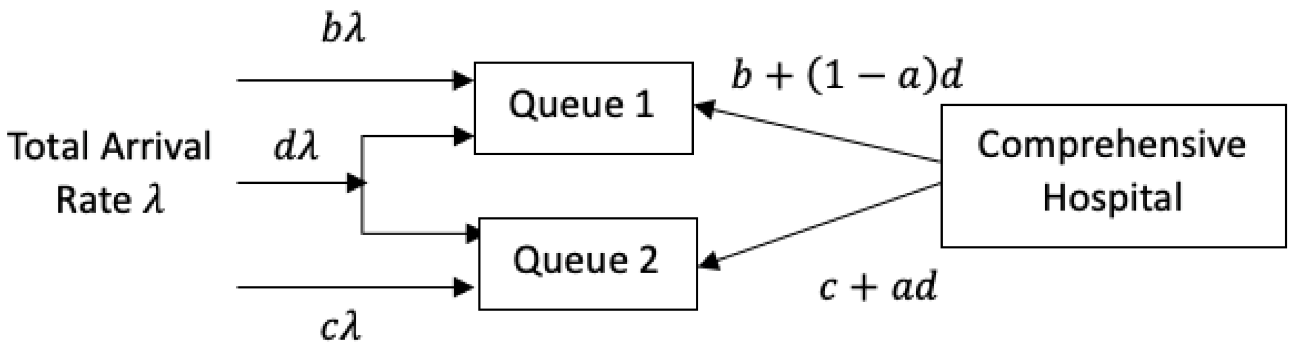
3.2. Model Introduction

First, we abstract the Chinese hierarchical healthcare system with a green channel into a two-tier queuing system. The arrival of patients follow as an $M/M/1$ queue, as shown in Figure 2. The total patient arrival rate is $\lambda$. In this system, there are two types of medical service. The first type is to join Queue 1 directly and wait for diagnosis and treatment at a comprehensive hospital. The second type is to join Queue 2 and receive primary diagnosis and treatment at the community health center. The community health center has a certain probability of successfully curing patients. If patients in Queue 2 are successfully treated at the community health center, they leave the queue; otherwise, they are referred to the comprehensive hospital.

We assume three types of patients. The first type directly joins Queue 1 for initial diagnosis at the comprehensive hospital with an arrival rate of $b\lambda$. The second type directly joins Queue 2 for initial diagnosis at the community health center with an arrival rate of $c\lambda$. The third type of customers choose the queue with the lowest cost based on the waiting time of both queues, and their arrival rate is $d\lambda$. The variables b, c, and d are considered exogenous and satisfy $b+c+d=1$.

In this system, we assume that the overall service rate of the comprehensive hospital is denoted by $\mu$, where $\mu$ > 0. To ensure the service of both queues, a service allocation mechanism is established as follows: when both Queue 1 and Queue 2 are non-empty, we allocate $b\mu$ services to Queue 1 and $c\mu$ services to Queue 2 patients. The remaining $d\mu$ service capacity is allocated to Queue 1 patients at a proportion of $(1-\alpha )$ and to Queue 2 patients at a proportion of $\alpha$, where $\alpha \in [0,1]$. This means Queue 1’s total service rate becomes $(b+(1-\alpha \left)d\right)\mu$, and Queue 2’s total service rate becomes $(c+\alpha d)\mu$. When one of the queues is empty, the comprehensive hospital will provide full-rate $\mu$ service to the other non-empty queue.

The objective is to discuss how to optimally allocate the remaining service capacity ($d\mu$) of the comprehensive hospital, i.e., to determine the optimal $\alpha$ that minimizes the operational cost of the hospital.

The number of patients waiting in Queue 1 and Queue 2 at time t is represented by $Q_1\left(t\right)$ and $Q_2\left(t\right)$. To simplify the referral process between the community health center and the comprehensive hospital, the service rate of the community health center is not considered. The reserved services of the community health center and the comprehensive hospital are integrated into a single service process. It is assumed that the number of patients who are successfully treated and leave Queue 2 by the community health center is a non-homogeneous Poisson process at a rate of $(1-r){[Q_2\left(t\right)-1]}^{+}$ at time t. Since patients in Queue 2 initially receive an initial diagnosis from the community health center, it can be assumed that the number of patients successfully treated by the community health center is a function of the queue length.

Assume the third type of patients choose the queue with the lowest cost based on their current estimated waiting time. Waiting time estimates provided by the service system are denoted as $W_1\left(t\right)$ and $W_2\left(t\right)$ for Queue 1 and Queue 2 at time t, respectively.

For Queue 1, the estimated waiting time $W_1\left(t\right)$ can be approximated as follows:

$$W_1\left(t\right):={\displaystyle \frac{Q_1\left(t\right)}{(b+(1-\alpha \left)d\right)\mu }}.$$

(1)

For Queue 2, the estimated waiting time $W_2\left(t\right)$ can be roughly estimated as follows:

$$W_2\left(t\right):={\displaystyle \frac{Q_2\left(t\right)}{(c+\alpha d)\mu }}.$$

(2)

Let ${\omega }_1$ and ${\omega }_2$ be positive constants representing the unit waiting time cost for the third type of patients in Queue 1 and Queue 2, respectively. Based on the discussion, the choice of patients arriving at the system at time t can be defined as follows:

$$\begin{array}{ccc}\hfill \mathrm{if}{\omega }_1{W}_1\left(t\right)& \le {\omega }_2{W}_2\left(t\right)\hfill & \hfill \mathrm{the}\mathrm{patient}\mathrm{joins}\mathrm{Queue}1,\end{array}$$

(3)

$$\begin{array}{ccc}\hfill \mathrm{if}{\omega }_1{W}_1\left(t\right)& >{\omega }_2{W}_2\left(t\right)\hfill & \hfill \mathrm{the}\mathrm{patient}\mathrm{joins}\mathrm{Queue}2.\end{array}$$

(4)

The objective is to optimize the operational cost of the entire service system by finding the optimal $\alpha$. We consider various cost components for patients waiting in Queue 1 and Queue 2, denoted as holding costs $h_1$ and $h_2$ (where $h_1$ < $h_2$), which are intended to penalize the inconvenience imposed by the service system on patients. Notably, the involvement of community health centers in Queue 2 makes the patient’s visit more cumbersome. Additionally, we account for the revenue generated from each patient successfully cured by the community health center, denoted as p ($p>0$). This revenue results from patients being treated at the community health center and subsequently leaving the system, effectively reducing the follow-up medical costs at the comprehensive hospital and thus lowering the overall operational costs of the system. Consequently, our total cost function can be expressed as follows:

$$\begin{array}{c}\hfill C(\alpha ,t)=h_1{\int }_0^t{Q}_1\left(s\right)ds+h_2{\int }_0^t{Q}_2\left(s\right)ds-pN\left({\int }_0^t(1-r){[Q_2\left(s\right)-1]}^{+}ds\right),\end{array}$$

(5)

where N is a standard Poisson process. The average total cost is as follows:

$$C\left(\alpha \right)=\underset{t\to \infty }{lim}{\displaystyle \frac{1}{t}}C(\alpha ,t).$$

(6)

The goal is to minimize the following:

$$\underset{\alpha \in [0,1]}{min}C\left(\alpha \right).$$

(7)

Within this optimization function, there is an implicit constraint equation, such as $Q_1,Q_2\ge 0$, which will be considered in the subsequent analysis.

3.3. System Analysis

In this section, we further detail the arrival and service processes of patients and establish their relationships with the queue lengths $Q_1$ and $Q_2$. We will then use Theorem 1 and Corollary 1 to approximate and optimize $Q_1$ and $Q_2$.

Let $\{u_i^1\ge 1\}$, $\{u_i^2\ge 1\}$, and $\{u_i^3\ge 1\}$ be a sequence of non-negative, independent, and identically distributed random variables with mean 1 and variance ${\sigma }_A^2$. Similarly, let $\{v_i^1\ge 1\}$ and $\{v_i^2\ge 1\}$ be a sequence of non-negative, independent, and identically distributed random variables with mean 1 and variance ${\sigma }_S^2$. We use $A_1\left(t\right)$, $A_2\left(t\right)$, $A_3\left(t\right)$, $S_1\left(t\right)$, and $S_2\left(t\right)$ to respectively represent the cumulative number of the first type of patients, the second type of patients, the third type of patients, patients served cumulatively in Queue 1 by the comprehensive hospital, and patients served cumulatively in Queue 2 by the comprehensive hospital from time 0 to time t. We have the following expressions:

$$\begin{array}{cc}\hfill A_1\left(t\right)& \equiv sup\left\{i\ge 0:{\Sigma }_{j=1}^i{u}_i^1\le b\lambda t\right\},\hfill \end{array}$$

(8)

$$\begin{array}{cc}\hfill A_2\left(t\right)& \equiv sup\left\{i\ge 0:{\Sigma }_{j=1}^i{u}_i^2\le c\lambda t\right\},\hfill \end{array}$$

(9)

$$\begin{array}{cc}\hfill A_3\left(t\right)& \equiv sup\left\{i\ge 0:{\Sigma }_{j=1}^i{u}_i^3\le d\lambda t\right\},\hfill \end{array}$$

(10)

$$\begin{array}{cc}\hfill S_1\left(t\right)& \equiv sup\left\{i\ge 0:{\Sigma }_{j=1}^i{v}_i^1\le \mu t\right\},\hfill \end{array}$$

(11)

$$\begin{array}{cc}\hfill S_2\left(t\right)& \equiv sup\left\{i\ge 0:{\Sigma }_{j=1}^i{v}_i^2\le \mu t\right\}\hfill \end{array}$$

(12)

Then, the queue lengths of Queue 1 and Queue 2 can be represented as follows:

$$\begin{array}{cc}\hfill Q_1\left(t\right)& =A_1\left(t\right)+A_{3,1}\left(t\right)-S_1\left(T_1\left(t\right)\right),\hfill \end{array}$$

(13)

$$\begin{array}{cc}\hfill Q_2\left(t\right)& =A_2\left(t\right)+A_{3,2}\left(t\right)-S_2\left(T_2\left(t\right)\right)-N\left({\int }_0^t\left(1-r\right){\left[Q_2\left(s\right)-1\right]}^{+}ds\right),\hfill \end{array}$$

(14)

where $A_{3,1}\left(t\right)$ and $A_{3,2}\left(t\right)$ represent the third type of patients choosing Queue 1 and Queue 2 with the following expressions:

$$\begin{array}{cc}\hfill A_{3,1}\left(t\right)& =\sum _{i=1}^{A\left(t\right)}1\left\{{\displaystyle \frac{{\omega }_1{Q}_1\left(t\right)}{\left(b+\left(1-\alpha \right)d\right)\mu }}\le {\displaystyle \frac{{\omega }_2{Q}_2\left(t\right)}{\left(c+\alpha d\right)\mu }}\right\},\hfill \end{array}$$

(15)

$$\begin{array}{cc}\hfill A_{3,2}\left(t\right)& =\sum _{i=1}^{A\left(t\right)}1\left\{{\displaystyle \frac{{\omega }_1{Q}_1\left(t\right)}{\left(b+\left(1-\alpha \right)d\right)\mu }}>{\displaystyle \frac{{\omega }_2{Q}_2\left(t\right)}{\left(c+\alpha d\right)\mu }}\right\}.\hfill \end{array}$$

(16)

$T1\left(t\right)$ and $T2\left(t\right)$ represent the busy times for Queue 1 and Queue 2, respectively, when both are working at the total service rate $\mu$. They are defined as follows:

$$\begin{array}{cc}\hfill T_1\left(t\right)& ={\int }_0^t{\displaystyle \frac{\left(b+\left(1-\alpha \right)d\right)1\left\{Q_1\left(s\right)>0\right\}}{b+\left(1-\alpha \right)d+\left(c+\alpha d\right)1\left\{Q_2\left(s\right)>0\right\}}}ds,\hfill \end{array}$$

(17)

$$\begin{array}{cc}\hfill T_2\left(t\right)& ={\int }_0^t{\displaystyle \frac{\left(c+\alpha d\right)1\left\{Q_2\left(s\right)>0\right\}}{c+\alpha d+\left(b+\left(1-\alpha \right)d\right)1\left\{Q_1\left(s\right)>0\right\}}}ds.\hfill \end{array}$$

(18)

We assume that the system operates under a heavy load, and we consider that the total service rate $\mu$ satisfies the following:

$$\mu :=\lambda -\sqrt{\lambda \theta },\theta \in \mathbb{R}.$$

(19)

The total queue length $Q\left(t\right)$ is defined as follows:

$$Q\left(t\right):=Q1\left(t\right)+Q2\left(t\right).$$

(20)

According to our allocation mechanism for the comprehensive hospital’s service, it only stops serving when the entire system is empty. Otherwise, the comprehensive hospital will provide service at a rate of $\mu$. We define $I\left(t\right)$ as the cumulative idle time of the comprehensive hospital from time 0 to t, which is given by the following:

$$I\left(t\right)={\int }_0^{t}1\left(Q\left(s\right)=0\right)ds.$$

(21)

Then, we have:

$$\begin{array}{cc}\hfill I\left(t\right)+T_1\left(t\right)+T_2\left(t\right)& =t,\hfill \end{array}$$

(22)

$$\begin{array}{cc}\hfill {\int }_0^{\infty }Q\left(s\right)dI\left(s\right)& =0.\hfill \end{array}$$

(23)

Theorem 1.

For any $T>0$, ${sup}_{0\le t\le T}\left|{\displaystyle \frac{{\omega }_1}{b+\left(1-\alpha \right)d}}{\tilde{Q}}_1\left(t\right)-{\displaystyle \frac{{\omega }_2}{c+\alpha d}}{\tilde{Q}}_2\left(t\right)\right|{\to }_{p}0$, as $\lambda \to \infty$.

Proof of Theorem 1.

We will begin by introducing some notations. We denote all the symbols with an upper (lower) index $\lambda$ to indicate that they depend on $\lambda$.

$$\begin{array}{cc}\hfill {\overline{\tau }}^{\lambda }\left(t\right)& \equiv {\displaystyle \frac{1}{\lambda }}{\int }_0^t\left(1-r\right){\left[Q_2^{\lambda }\left(s\right)-1\right]}^{+}ds,\hfill \end{array}$$

(24)

$$\begin{array}{cc}\hfill {\tilde{A}}_1^{\lambda }\left(t\right)& \equiv {\displaystyle \frac{A_1^{\lambda }\left(t\right)-b\lambda t}{\sqrt{\lambda }}},\hfill \end{array}$$

(25)

$$\begin{array}{cc}\hfill {\tilde{A}}_2^{\lambda }\left(t\right)& \equiv {\displaystyle \frac{A_2^{\lambda }\left(t\right)-c\lambda t}{\sqrt{\lambda }}},\hfill \end{array}$$

(26)

$$\begin{array}{cc}\hfill {\tilde{A}}_3^{\lambda }\left(t\right)& \equiv {\displaystyle \frac{A_3^{\lambda }\left(t\right)-d\lambda t}{\sqrt{\lambda }}},\hfill \end{array}$$

(27)

$$\begin{array}{cc}\hfill {\tilde{S}}_1^{\lambda }\left(t\right)& \equiv {\displaystyle \frac{S_1^{\lambda }\left(t\right)-\mu t}{\sqrt{\lambda }}},\hfill \end{array}$$

(28)

$$\begin{array}{cc}\hfill {\tilde{S}}_2^{\lambda }\left(t\right)& \equiv {\displaystyle \frac{S_2^{\lambda }\left(t\right)-\mu t}{\sqrt{\lambda }}},\hfill \end{array}$$

(29)

$$\begin{array}{cc}\hfill {\tilde{N}}^{\lambda }\left(t\right)& \equiv {\displaystyle \frac{N\left(\lambda t\right)-\lambda t}{\sqrt{\lambda }}},\hfill \end{array}$$

(30)

$$\begin{array}{cc}\hfill {\tilde{Q}}_1^{\lambda }\left(t\right)& \equiv {\displaystyle \frac{Q_1^{\lambda }\left(t\right)}{\sqrt{\lambda }}},\hfill \end{array}$$

(31)

$$\begin{array}{cc}\hfill {\tilde{Q}}_2^{\lambda }\left(t\right)& \equiv {\displaystyle \frac{Q_2^{\lambda }\left(t\right)}{\sqrt{\lambda }}},\hfill \end{array}$$

(32)

$$\begin{array}{cc}\hfill {\tilde{Q}}^{\lambda }\left(t\right)& \equiv {\displaystyle \frac{Q^{\lambda }\left(t\right)}{\sqrt{\lambda }}},\hfill \end{array}$$

(33)

$$\begin{array}{cc}\hfill {\tilde{I}}^{\lambda }\left(t\right)& \equiv \sqrt{\lambda }{I}^{\lambda }\left(t\right).\hfill \end{array}$$

(34)

We also define the following:

$$\begin{array}{cc}\hfill {\tilde{U}}_1^{\lambda }\left(t,s,u,v\right)& \equiv -{\displaystyle \frac{{\omega }_1}{b+\left(1-\alpha \right)d}}\left[{\tilde{S}}_1^{\lambda }\left(u+\left(b+\left(1-\alpha \right)d\right)\left(t-s\right)\right)-{\tilde{S}}_1^{\lambda }\left(u\right)\right]\hfill \\ \hfill & +{\displaystyle \frac{{\omega }_2}{c+\alpha d}}\left[{\tilde{S}}_2^{\lambda }\left(v+\left(c+\alpha d\right)\left(t-s\right)\right)-{\tilde{S}}_2^{\lambda }\left(v\right)\right]+{\displaystyle \frac{{\omega }_1}{b+\left(1-\alpha \right)d}}\left[{\tilde{A}}_1^{\lambda }\left(t\right)-{\tilde{A}}_1^{\lambda }\left(s\right)\right]\hfill \\ \hfill & -{\displaystyle \frac{{\omega }_2}{c+\alpha d}}\left[{\tilde{A}}_2^{\lambda }\left(t\right)-{\tilde{A}}_2^{\lambda }\left(s\right)+{\tilde{A}}_3^{\lambda }\left(t\right)-{\tilde{A}}_3^{\lambda }\left(s\right)\right]\hfill \\ \hfill & +\left[{\displaystyle \frac{\theta }{\sqrt{\lambda }}}\left({\omega }_2-{\omega }_1\right)+{\displaystyle \frac{\left(\alpha -1\right)d{\omega }_1}{b+\left(1-\alpha \right)d}}+{\displaystyle \frac{\left(\alpha -1\right)d{\omega }_2}{c+\alpha d}}\right]\sqrt{\lambda }\left(t-s\right),\hfill \end{array}$$

(35)

$$\begin{array}{cc}\hfill {\tilde{U}}_2^{\lambda }\left(t,s,u,v\right)& \equiv {\displaystyle \frac{{\omega }_1}{b+\left(1-\alpha \right)d}}\left[{\tilde{S}}_1^{\lambda }\left(u+\left(b+\left(1-\alpha \right)d\right)\left(t-s\right)\right)-{\tilde{S}}_1^{\lambda }\left(u\right)\right]\hfill \\ \hfill & -{\displaystyle \frac{{\omega }_2}{c+\alpha d}}\left[{\tilde{S}}_2^{\lambda }\left(v+\left(c+\alpha d\right)\left(t-s\right)\right)-{\tilde{S}}_2^{\lambda }\left(v\right)\right]+{\displaystyle \frac{{\omega }_2}{c+\alpha d}}\left[{\tilde{A}}_2^{\lambda }\left(t\right)-{\tilde{A}}_2^{\lambda }\left(s\right)\right]\hfill \\ \hfill & -{\displaystyle \frac{{\omega }_1}{b+\left(1-\alpha \right)d}}\left[{\tilde{A}}_1^{\lambda }\left(t\right)-{\tilde{A}}_1^{\lambda }\left(s\right)+{\tilde{A}}_3^{\lambda }\left(t\right)-{\tilde{A}}_3^{\lambda }\left(s\right)\right]\hfill \\ \hfill & +\left[{\displaystyle \frac{\theta }{\sqrt{\mu }}}\left({\omega }_1-{\omega }_2\right)-{\displaystyle \frac{\alpha d{\omega }_1}{b+\left(1-\alpha \right)d}}-{\displaystyle \frac{\alpha c{\omega }_2}{c+\alpha d}}\right]\sqrt{\lambda }\left(t-s\right).\hfill \end{array}$$

(36)

We need to prove that for any $ϵ>0$,

$$P\left(\underset{0\le t\le T}{sup}\left|{\displaystyle \frac{{\omega }_1}{b+\left(1-\alpha \right)d}}{\tilde{Q}}_1^{\lambda }\left(t\right)-{\displaystyle \frac{{\omega }_2}{c+\alpha d}}{\tilde{Q}}_2^{\lambda }\left(t\right)\right|>\epsilon \right)\to 0,\mathrm{when}\lambda \to \infty .$$

(37)

To prove (37), let us fix $ϵ$.

$$\begin{array}{cc}\hfill {\xi }_{\lambda }& \equiv inf\left\{t\ge 0:\left|{\displaystyle \frac{{\omega }_1}{b+\left(1-\alpha \right)d}}{\tilde{Q}}_1^{\lambda }\left(t\right)-{\displaystyle \frac{{\omega }_2}{c+\alpha d}}{\tilde{Q}}_2^{\lambda }\left(t\right)\right|>\epsilon \right\},\hfill \end{array}$$

(38)

$$\begin{array}{cc}\hfill {\xi }_{\lambda }^{*}& \equiv sup\left\{t\ge 0:\left|{\displaystyle \frac{{\omega }_1}{b+\left(1-\alpha \right)d}}{\tilde{Q}}_1^{\lambda }\left(t\right)-{\displaystyle \frac{{\omega }_2}{c+\alpha d}}{\tilde{Q}}_2^{\lambda }\left(t\right)\right|\le {\displaystyle \frac{\epsilon }{2}}\right\}.\hfill \end{array}$$

(39)

First, let us assume ${\displaystyle \frac{{\omega }_1}{b+\left(1-\alpha \right)d}}{\tilde{Q}}_1^{\lambda }\left({\xi }_{\lambda }^{*}\right)>{\displaystyle \frac{{\omega }_2}{c+\alpha d}}{\tilde{Q}}_2^{\lambda }\left({\xi }_{\lambda }^{*}\right)$; then, when ${\xi }_{\lambda }^{*}\le t\le {\xi }_{\lambda },$ all the type 3 patients join Queue 2, i.e.,

$$\begin{array}{cc}\hfill & \left|{\displaystyle \frac{{\omega }_1}{b+\left(1-\alpha \right)d}}{\tilde{Q}}_1^{\lambda }\left(t\right)-{\displaystyle \frac{{\omega }_2}{c+\alpha d}}{\tilde{Q}}_2^{\lambda }\left(t\right)\right|\hfill \\ \hfill & ={\displaystyle \frac{{\omega }_1}{b+\left(1-\alpha \right)d}}{\tilde{Q}}_1^{\lambda }\left({\xi }_{\lambda }^{*}-\right)-{\displaystyle \frac{{\omega }_2}{c+\alpha d}}{\tilde{Q}}_2^{\lambda }\left({\xi }_{\lambda }^{*}-\right)+{\displaystyle \frac{{\omega }_1}{b+\left(1-\alpha \right)d}}\left[{\tilde{A}}_1^{\lambda }\left(t\right)-{\tilde{A}}_1^{\lambda }\left({\xi }_{\lambda }^{*}-\right)+b\sqrt{\lambda }\left(t-{\xi }_{\lambda }^{*}\right)\right]\hfill \\ \hfill & -{\displaystyle \frac{{\omega }_1}{b+\left(1-\alpha \right)d}}{\displaystyle \frac{1}{\sqrt{\lambda }}}\left[S_1^{\lambda }\left(T_1\left(t\right)\right)-S_1^{\lambda }\left(T_1\left({\xi }_{\lambda }^{*}-\right)\right)\right]+{\displaystyle \frac{{\omega }_2}{c+\alpha d}}{\displaystyle \frac{1}{\sqrt{\lambda }}}\left[S_2^{\lambda }\left(T_2\left(t\right)\right)-S_2^{\lambda }\left(T_2\left({\xi }_{\lambda }^{*}-\right)\right)\right]\hfill \\ \hfill & -{\displaystyle \frac{{\omega }_2}{c+\alpha d}}\left[{\tilde{A}}_2^{\lambda }\left(t\right)-{\tilde{A}}_2^{\lambda }\left({\xi }_{\lambda }^{*}-\right)+{\tilde{A}}_3^{\lambda }\left(t\right)-{\tilde{A}}_3^{\lambda }\left({\xi }_{\lambda }^{*}-\right)+\left(c+d\right)\sqrt{\lambda }\left(t-{\xi }_{\lambda }^{*}\right)\right]\hfill \\ \hfill & +{\displaystyle \frac{{\omega }_2}{c+\alpha d}}{\displaystyle \frac{1}{\sqrt{\lambda }}}\left[N\left({\int }_0^t\left(1-r\right){\left[Q_2^{\lambda }\left(s\right)-1\right]}^{+}ds\right)-N\left({\int }_0^{{\xi }_{\lambda }^{*}-}\left(1-r\right){\left[Q_2^{\lambda }\left(s\right)-1\right]}^{+}ds\right)\right].\hfill \end{array}$$

(40)

Therefore, Queue 1 is nonempty during the time interval $\left[{\xi }_{\lambda }^{*},{\xi }_{\lambda }\right]$, i.e.,

$$T_1^{\lambda }\left(t\right)-T_1^{\lambda }\left({\xi }_{\lambda }^{*}-\right)\ge \left(b+\left(1-\alpha \right)d\right)\left(t-{\xi }_{\lambda }^{*}\right).$$

(41)

But, Queue 2 can be empty during the time interval $\left[{\xi }_{\lambda }^{*},{\xi }_{\lambda }\right]$, i.e.,

$$T_2^{\lambda }\left(t\right)-T_2^{\lambda }\left({\xi }_{\lambda }^{*}-\right)\le \left(c+\alpha d\right)\left(t-{\xi }_{\lambda }^{*}\right).$$

(42)

Because $S_1,S_2$ are non-decreasing process, we have

$$\begin{array}{ccc}& & S_1^{\lambda }\left(T_1^{\lambda }\left(t\right)\right)-S_1^{\lambda }\left(T_1^{\lambda }\left({\xi }^{*}-\right)\right)\hfill \\ & \ge & \sqrt{\lambda }({\tilde{S}}_1^{\lambda }\left(T_1^{\lambda }\left({\xi }_{\lambda }^{*}-\right)+\left(b+\left(1-\alpha \right)d\right)\left(t-{\xi }_{\lambda }^{*}\right)\right)-{\tilde{S}}_1^{\lambda }\left(T_1^{\lambda }\left({\xi }_{\lambda }^{*}-\right)\right)\hfill \\ & & +\left(b+\left(1-\alpha \right)d\right)\left(\sqrt{\lambda }+\theta \right)\left(t-{\xi }_{\lambda }^{*}\right)),\hfill \end{array}$$

(43)

and

$$\begin{array}{cc}\hfill & S_2^{\lambda }\left(T_2^{\lambda }\left(t\right)\right)-S_2^{\lambda }\left(T_2^{\lambda }\left({\xi }_{\lambda }^{*}-\right)\right)\hfill \\ \hfill & \le \sqrt{\lambda }\left({\tilde{S}}_2^{\lambda }\left(T_2^{\lambda }\left({\xi }_{\lambda }^{*}-\right)+\left(c+\alpha d\right)\left(t-{\xi }_{\lambda }^{*}\right)\right)-{\tilde{S}}_2^{\lambda }\left(T_2^{\lambda }\left({\xi }_{\lambda }^{*}-\right)\right)+\left(c+\alpha d\right)\left(\sqrt{\lambda }+\theta \right)\left(t-{\xi }_{\lambda }^{*}\right)\right).\hfill \end{array}$$

(44)

Based on the definition of ${\xi }_{\lambda }^{*}$ (39), (43), and (44), we have

$$\begin{array}{cc}\hfill & \left|{\displaystyle \frac{{\omega }_1}{b+\left(1-\alpha \right)d}}{\tilde{Q}}_1^{\lambda }\left(t\right)-{\displaystyle \frac{{\omega }_2}{c+\alpha d}}{\tilde{Q}}_2^{\lambda }\left(t\right)\right|\hfill \\ \hfill & \le {\displaystyle \frac{\epsilon }{2}}+{\tilde{U}}_1^{\lambda }\left(t,{\xi }^{*}-,T_1^{\lambda }\left({\xi }_{\lambda }^{*}-\right),T_2^{\lambda }\left({\xi }_{\lambda }^{*}-\right)\right)\hfill \\ \hfill & +{\displaystyle \frac{{\omega }_2}{c+\alpha d}}{\displaystyle \frac{1}{\sqrt{\lambda }}}\left[N\left({\int }_0^t\left(1-r\right){\left[Q_2^{\lambda }\left(s\right)-1\right]}^{+}ds\right)-N\left({\int }_0^{{\xi }_{\lambda }^{*}-}\left(1-r\right){\left[Q_2^{\lambda }\left(s\right)-1\right]}^{+}ds\right)\right],\hfill \end{array}$$

(45)

where the expression for ${\tilde{U}}_1^{\lambda }\left(t,s,u,v\right)$ is given in (35).

Now, assuming ${\displaystyle \frac{{\omega }_1}{b+\left(1-\alpha \right)d}}{\tilde{Q}}_1^{\lambda }\left({\xi }_{\lambda }^{*}\right)\le {\displaystyle \frac{{\omega }_2}{c+\alpha d}}{\tilde{Q}}_2^{\lambda }\left({\xi }_{\lambda }^{*}\right)$, it means that all third type patients join Queue 1, and similarly,

$$\begin{array}{cc}\hfill & \left|{\displaystyle \frac{{\omega }_1}{b+\left(1-\alpha \right)d}}{\tilde{Q}}_1^{\lambda }\left(t\right)-{\displaystyle \frac{{\omega }_2}{c+\alpha d}}{\tilde{Q}}_2^{\lambda }\left(t\right)\right|\hfill \\ \hfill & =-{\displaystyle \frac{{\omega }_1}{b+\left(1-\alpha \right)d}}{\tilde{Q}}_1^{\lambda }\left({\xi }_{\lambda }^{*}-\right)+{\displaystyle \frac{{\omega }_2}{c+\alpha d}}{\tilde{Q}}_2^{\lambda }\left({\xi }_{\lambda }^{*}-\right)+{\displaystyle \frac{{\omega }_2}{c+\alpha d}}\left[{\tilde{A}}_2^{\lambda }\left(t\right)-{\tilde{A}}_2^{\lambda }\left({\xi }_{\lambda }^{*}-\right)+c\sqrt{\lambda }\left(t-{\xi }_{\lambda }^{*}\right)\right]\hfill \\ \hfill & +{\displaystyle \frac{{\omega }_1}{b+\left(1-\alpha \right)d}}{\displaystyle \frac{1}{\sqrt{\lambda }}}\left[S_1^{\lambda }\left(T_1\left(t\right)\right)-S_1^{\lambda }\left(T_1\left({\xi }_{\lambda }^{*}-\right)\right)\right]-{\displaystyle \frac{{\omega }_2}{c+\alpha d}}{\displaystyle \frac{1}{\sqrt{\lambda }}}\left[S_2^{\lambda }\left(T_2\left(t\right)\right)-S_2^{\lambda }\left(T_2\left({\xi }_{\lambda }^{*}-\right)\right)\right]\hfill \\ \hfill & -{\displaystyle \frac{{\omega }_1}{b+\left(1-\alpha \right)d}}\left[{\tilde{A}}_1^{\lambda }\left(t\right)-{\tilde{A}}_1^{\lambda }\left({\xi }_{\lambda }^{*}-\right)+{\tilde{A}}_3^{\lambda }\left(t\right)-{\tilde{A}}_3^{\lambda }\left({\xi }_{\lambda }^{*}-\right)+\left(b+d\right)\sqrt{\lambda }\left(t-{\xi }_{\lambda }^{*}\right)\right]\hfill \\ \hfill & -{\displaystyle \frac{{\omega }_2}{c+\alpha d}}{\displaystyle \frac{1}{\sqrt{\lambda }}}\left[N\left({\int }_0^t\left(1-r\right){\left[Q_2^{\lambda }\left(s\right)-1\right]}^{+}ds\right)-N\left({\int }_0^{{\xi }_{\lambda }^{*}-}\left(1-r\right){\left[Q_2^{\lambda }\left(s\right)-1\right]}^{+}ds\right)\right].\hfill \end{array}$$

(46)

All type 3 patients join Queue 1, so Queue 1 might be empty during the time interval $\left[{\xi }_{\lambda }^{*},{\xi }_{\lambda }\right]$, i.e.,

$$T_1^{\lambda }\left(t\right)-T_1^{\lambda }\left({\xi }_{\lambda }^{*}-\right)\le \left(b+\left(1-\alpha \right)d\right)\left(t-{\xi }_{\lambda }^{*}\right).$$

(47)

Furthermore, Queue 2 is not empty during the time interval $[{\xi }_{\lambda }^{*},{\xi }_{\lambda }]$, so we have

$$T_{\lambda }^{\sim }\left(t\right)-T_{\lambda }^{\sim }({\xi }^{*}-)\ge (c+\alpha d)(t-{\xi }^{*}).$$

Again, based on the fact that $S_1$ and $S_2$ are non-decreasing processes, we have

$$\begin{array}{ccc}& & S_1^{\lambda }\left(T_1^{\lambda }\left(t\right)\right)-S_1^{\lambda }\left(T_1^{\lambda }\left({\xi }_{\lambda }^{*}-\right)\right)\hfill \\ & \le & \sqrt{\lambda }({\tilde{S}}_1^{\lambda }\left(T_1^{\lambda }\left({\xi }_{\lambda }^{*}-\right)+\left(b+\left(1-\alpha \right)d\right)\left(t-{\xi }_{\lambda }^{*}\right)\right)-{\tilde{S}}_1^{\lambda }\left(T_1^{\lambda }\left({\xi }_{\lambda }^{*}-\right)\right)\hfill \\ & & +\left(b+\left(1-\alpha \right)d\right)\left(\sqrt{\lambda }+\theta \right)\left(t-{\xi }_{\lambda }^{*}\right)),\hfill \end{array}$$

(48)

and

$$\begin{array}{cc}\hfill & S_2^{\lambda }\left(T_2^{\lambda }\left(t\right)\right)-S_2^{\lambda }\left(T_2^{\lambda }\left({\xi }_{\lambda }^{*}-\right)\right)\hfill \\ \hfill & \ge \sqrt{\lambda }\left({\tilde{S}}_2^{\lambda }\left(T_2^{\lambda }\left({\xi }_{\lambda }^{*}-\right)+\left(c+\alpha d\right)\left(t-{\xi }_{\lambda }^{*}\right)\right)-{\tilde{S}}_2^{\lambda }\left(T_2^{\lambda }\left({\xi }_{\lambda }^{*}-\right)\right)+\left(c+\alpha d\right)\left(\sqrt{\lambda }+\theta \right)\left(t-{\xi }_{\lambda }^{*}\right)\right).\hfill \end{array}$$

(49)

Similarly, we have

$$\begin{array}{cc}\hfill & \left|{\displaystyle \frac{{\omega }_1}{b+\left(1-\alpha \right)d}}{\tilde{Q}}_1^{\lambda }\left(t\right)-{\displaystyle \frac{{\omega }_2}{c+\alpha d}}{\tilde{Q}}_2^{\lambda }\left(t\right)\right|\hfill \\ \hfill & \le {\displaystyle \frac{\epsilon }{2}}+{\tilde{U}}_2^{\lambda }\left(t,{\xi }_{\lambda }^{*}-,T_1^{\lambda }\left({\xi }_{\lambda }^{*}-\right),T_2^{\lambda }\left({\xi }_{\lambda }^{*}-\right)\right)\hfill \\ \hfill & -{\displaystyle \frac{{\omega }_2}{c+\alpha d}}{\displaystyle \frac{1}{\sqrt{\lambda }}}\left[N\left({\int }_0^t\left(1-r\right){\left[Q_2^{\lambda }\left(s\right)-1\right]}^{+}ds\right)-N\left({\int }_0^{{\xi }_{\lambda }^{*}-}\left(1-r\right){\left[Q_2^{\lambda }\left(s\right)-1\right]}^{+}ds\right)\right],\hfill \end{array}$$

(50)

where ${\tilde{U}}_2^{\lambda }\left(t,s,u,v\right)$ follows (36).

Note that, when process N is non-negative, we have

$$\begin{array}{cc}\hfill & \left|{\displaystyle \frac{{\omega }_1}{b+\left(1-\alpha \right)d}}{\tilde{Q}}_1^{\lambda }\left(t\right)-{\displaystyle \frac{{\omega }_2}{c+\alpha d}}{\tilde{Q}}_2^{\lambda }\left(t\right)\right|\hfill \\ \hfill & \le {\displaystyle \frac{\epsilon }{2}}+max\{{\tilde{U}}_1^{\lambda }\left(t,{\xi }_{\lambda }^{*}-,T_1^{\lambda }\left({\xi }_{\lambda }^{*}-\right),T_2^{\lambda }\left({\xi }_{\lambda }^{*}-\right)\right),{\tilde{U}}_2^{\lambda }\left(t,{\xi }_{\lambda }^{*}-,T_1^{\lambda }\left({\xi }_{\lambda }^{*}-\right),T_2^{\lambda }\left({\xi }_{\lambda }^{*}-\right)\right)\}\hfill \\ \hfill & +{\displaystyle \frac{{\omega }_2}{c+\alpha d}}{\displaystyle \frac{1}{\sqrt{\lambda }}}\left[N\left({\int }_0^t\left(1-r\right){\left[Q_2^{\lambda }\left(s\right)-1\right]}^{+}ds\right)-N\left({\int }_0^{{\xi }_{\lambda }^{*}-}\left(1-r\right){\left[Q_2^{\lambda }\left(s\right)-1\right]}^{+}ds\right)\right].\hfill \end{array}$$

(51)

Finally, the left-hand side of (37) can be bounded as follows:

$$\begin{array}{ccc}& & P\left(\underset{0\le t\le T}{sup}\left|{\displaystyle \frac{{\omega }_1}{b+\left(1-\alpha \right)d}}{\tilde{Q}}_1^{\lambda }\left(t\right)-{\displaystyle \frac{{\omega }_2}{c+\alpha d}}{\tilde{Q}}_2^{\lambda }\left(t\right)\right|>\epsilon \right)\hfill \\ & \le & P\left(\begin{array}{c}max\{{\tilde{U}}_1^{\lambda }\left(t,{\xi }_{\lambda }^{*}-,T_1^{\lambda }\left({\xi }_{\lambda }^{*}-\right),T_2^{\lambda }\left({\xi }_{\lambda }^{*}-\right)\right),{\tilde{U}}_2^{\lambda }\left(t,{\xi }_{\lambda }^{*}-,T_1^{\lambda }\left({\xi }_{\lambda }^{*}-\right),T_2^{\lambda }\left({\xi }_{\lambda }^{*}-\right)\right)\}\\ +{\displaystyle \frac{{\omega }_2}{c+\alpha d}}{\displaystyle \frac{1}{\sqrt{\lambda }}}\left[N\left({\int }_0^t\left(1-r\right){\left[Q_2^{\lambda }\left(s\right)-1\right]}^{+}ds\right)-N\left({\int }_0^{{\xi }_{\lambda }^{*}-}\left(1-r\right){\left[Q_2^{\lambda }\left(s\right)-1\right]}^{+}ds\right)\right]\end{array}>{\displaystyle \frac{\epsilon }{2}}\right).\hfill \end{array}$$

(52)

For any small $\eta$, we will show that the left-hand-side of (52) is less than $\eta$ for sufficiently large $\lambda$.

The remaining proof is similar to the Technical Appendix of [11], which will not be elaborated upon. □

By Theorem 1 and Theorem 1(b) in [11], we have the following Corollary.

Corollary 1.

When $\lambda \to \infty$, we have

$$\begin{array}{ccc}\hfill {\displaystyle \frac{Q_1^{\lambda }}{\sqrt{\lambda }}}& \Rightarrow & {\displaystyle \frac{\left(b+\left(1-\alpha \right)d\right){\omega }_2}{\left(c+\alpha d\right){\omega }_1+\left(b+\left(1-\alpha \right)d\right){\omega }_2}}\tilde{Q},\hfill \end{array}$$

(53)

$$\begin{array}{ccc}\hfill {\displaystyle \frac{Q_2^{\lambda }}{\sqrt{\lambda }}}& \Rightarrow & {\displaystyle \frac{\left(c+\alpha d\right){\omega }_1}{\left(c+\alpha d\right){\omega }_1+\left(b+\left(1-\alpha \right)d\right){\omega }_2}}\tilde{Q},\hfill \end{array}$$

(54)

$$\begin{array}{ccc}\hfill {\displaystyle \frac{N\left({\int }_0^{·}\left(1-r\right){\left[Q_2^{\lambda }\left(s\right)-1\right]}^{+}ds\right)}{\sqrt{\lambda }}}& \Rightarrow & {\displaystyle \frac{\left(1-r\right)\left(c+\alpha d\right){\omega }_1}{\left(c+\alpha d\right){\omega }_1+\left(b+\left(1-\alpha \right)d\right){\omega }_2}}{\int }_0^{·}\tilde{Q}\left(s\right)ds,\hfill \end{array}$$

(55)

where $\tilde{Q}\left(t\right)$ satisfies

$$\tilde{Q}\left(t\right)=\tilde{X}\left(t\right)-{\displaystyle \frac{\left(1-r\right)\left(c+\alpha d\right){\omega }_1}{\left(c+\alpha d\right){\omega }_1+\left(b+\left(1-\alpha \right)d\right){\omega }_2}}{\int }_0^t\tilde{Q}\left(s\right)ds+\tilde{I}\left(t\right)\ge 0.$$

(56)

$\tilde{X}\left(t\right)$ is a Brownian motion with drift θ, and variance ${\sigma }^2:={\sigma }_A^2+{\sigma }_S^2$; $\tilde{I}\left(t\right)$ is a non-decreasing process that satisfies the folloing:

$$\begin{array}{ccc}\hfill \tilde{I}\left(0\right)& =& 0\hfill \end{array}$$

(57)

$$\begin{array}{ccc}\hfill {\int }_0^{\infty }\tilde{Q}\left(s\right)d\tilde{I}\left(s\right)& =& 0.\hfill \end{array}$$

(58)

Therefore, based on Corollary 1, (5) can be estimated as follows:

$$\begin{array}{ccc}\hfill {\displaystyle \frac{C\left(\alpha ,t\right)}{\sqrt{\lambda }}}& \approx & \left({\displaystyle \frac{h_1\left(b+\left(1-\alpha \right)d\right){\omega }_2}{\left(c+\alpha d\right){\omega }_1+\left(b+\left(1-\alpha \right)d\right){\omega }_2}}+{\displaystyle \frac{\left(h_2-p\left(1-r\right)\right)\left(c+\alpha d\right){\omega }_1}{\left(c+\alpha d\right){\omega }_1+\left(b+\left(1-\alpha \right)d\right){\omega }_2}}\right)\hfill \\ & & \times {\int }_0^t\tilde{Q}\left(s\right)ds.\hfill \end{array}$$

(59)

When $t\to \infty ,\tilde{Q}\left(\infty \right)$ has stationary distribution. Therefore,

$$P\left(\underset{t\to \infty }{lim}{\int }_0^t\tilde{Q}\left(s\right)ds\to E\left[\tilde{Q}\left(\infty \right)\right]\right)=1.$$

(60)

Combined with (59), (6) can be approximated as follows:

$${\displaystyle \frac{C\left(\alpha \right)}{\sqrt{\lambda }}}\approx \left({\displaystyle \frac{h_1\left(b+\left(1-\alpha \right)d\right){\omega }_2}{\left(c+\alpha d\right){\omega }_1+\left(b+\left(1-\alpha \right)d\right){\omega }_2}}+{\displaystyle \frac{\left(h_2-p\left(1-r\right)\right)\left(c+\alpha d\right){\omega }_1}{\left(c+\alpha d\right){\omega }_1+\left(b+\left(1-\alpha \right)d\right){\omega }_2}}\right)E\left[\tilde{Q}\left(\infty \right)\right].$$

(61)

Define

$$\kappa :={\displaystyle \frac{\left(1-r\right)\left(c+\alpha d\right){\omega }_1}{\left(c+\alpha d\right){\omega }_1+\left(b+\left(1-\alpha \right)d\right){\omega }_2}}.$$

(62)

According to Proposition 1 in [20], the stationary expectation of $\tilde{Q}$

$$E\left[\tilde{Q}\left(\infty \right)\right]={\displaystyle \frac{\theta }{\kappa }}+{\displaystyle \frac{\sigma }{\sqrt{2\kappa }}}{\displaystyle \frac{\varphi \left(\left(-\theta /\sigma \sqrt{2/\kappa }\right)\right)}{1-\Phi \left(\left(-\theta /\sigma \sqrt{2/\kappa }\right)\right)}},$$

(63)

where $\varphi ,\Phi$ is probability density function and cumulative probably function of standard normal distribution. Therefore, the optimization problem in (7) can be estimated as follows:

$$\underset{\alpha \in \left[0,1\right]}{min}\tilde{C}\left(\alpha \right),$$

(64)

where

$$\begin{array}{ccc}\hfill \tilde{C}\left(\alpha \right)& =& \left({\displaystyle \frac{h_1\left(b+\left(1-\alpha \right)d\right){\omega }_2}{\left(c+\alpha d\right){\omega }_1+\left(b+\left(1-\alpha \right)d\right){\omega }_2}}+{\displaystyle \frac{\left(h_2-p\left(1-r\right)\right)\left(c+\alpha d\right){\omega }_1}{\left(c+\alpha d\right){\omega }_1+\left(b+\left(1-\alpha \right)d\right){\omega }_2}}\right)\hfill \\ & & \times \left({\displaystyle \frac{\theta }{\kappa }}+{\displaystyle \frac{\sigma }{\sqrt{2\kappa }}}{\displaystyle \frac{\varphi \left(\left(-\theta /\sigma \sqrt{2/\kappa }\right)\right)}{1-\Phi \left(\left(-\theta /\sigma \sqrt{2/\kappa }\right)\right)}}\right).\hfill \end{array}$$

(65)

Let ${\tilde{\alpha }}^{*}$ be the optimal solution of approximates (64), and let ${\alpha }^{*}$ be the optimal solution of original question (7). If we can show ${\tilde{\alpha }}^{*}\approx {\alpha }^{*}$, then our estimates are accurate.

4. Optimization of Approximation Problem

In this section, we present the optimal solution, denoted as ${\tilde{\alpha }}^{*}$, obtained through the optimization of the approximation problem (64). We seek the optimal solution within the closed interval [0, 1], and it is guaranteed to have a feasible solution. We consider two scenarios: when $\theta =0$ and when $\theta \ne 0$. For the former scenario, this corresponds to a situation where the arrival rate is equal to the service rate, and ${\tilde{\alpha }}^{*}$ has a closed-form solution. In the latter scenario, where the arrival rate is not equal to the service rate, we employ numerical methods to determine ${\tilde{\alpha }}^{*}$. Furthermore, we conduct graphical analyses to comprehend the impact of parameters, such as $h_2$, $h_1$, p, ${\omega }_1$, and ${\omega }_2$, on the optimal point ${\tilde{\alpha }}^{*}$ and its practical significance.

4.1. Arrival Rate Is Equal to Service Rate

In this subsection, we consider the optimal solution when $\theta =0$, i.e., $\mu =\lambda$, and the system is under heavy traffic, then (65) can be simplified as follows:

$$\tilde{C}\left(\alpha \right)={\displaystyle \frac{\sigma h_1}{\sqrt{\pi \left(1-r\right)}}}{\left(1+{\displaystyle \frac{b+\left(1-\alpha \right)d}{c+\alpha d}}{\displaystyle \frac{{\omega }_2}{{\omega }_1}}\right)}^{-1/2}\left({\displaystyle \frac{b+\left(1-\alpha \right)d}{c+\alpha d}}{\displaystyle \frac{{\omega }_2}{{\omega }_1}}+{\displaystyle \frac{h_2-p\left(1-r\right)}{h_1}}\right).$$

(66)

(66) has the following first-order derivative:

$$\begin{array}{ccc}\hfill {\tilde{C}}^{\prime }\left(\alpha \right)& =& {\displaystyle \frac{\sigma h_{1}d}{2\sqrt{\pi \left(1-r\right)}{\left(c+\alpha d\right)}^3}}{\left({\displaystyle \frac{{\omega }_2}{{\omega }_1}}\right)}^2{\left(1+{\displaystyle \frac{b+\left(1-\alpha \right)d}{c+\alpha d}}{\displaystyle \frac{{\omega }_2}{{\omega }_1}}\right)}^{-3/2}\hfill \\ & & \times \left(d\left(1-{\displaystyle \frac{{\omega }_1}{{\omega }_2}}\left(2-{\displaystyle \frac{h_2-p\left(1-r\right)}{h_1}}\right)\right)\alpha -1+\left(1-{\displaystyle \frac{{\omega }_1}{{\omega }_2}}\left(2-{\displaystyle \frac{h_2-p\left(1-r\right)}{h_1}}\right)\right)c\right).\hfill \end{array}$$

(67)

By finding the zero points of the first derivative of (67) and considering the sign of the second derivative from (66), we obtain a closed-form solution for ${\tilde{\alpha }}^{*}$:

$${\tilde{\alpha }}^{*}=\left\{\begin{array}{cc}0& {\displaystyle \frac{h_2-p\left(1-r\right)}{h_1}}\ge 2+{\displaystyle \frac{1-c}{c}}{\displaystyle \frac{{\omega }_2}{{\omega }_1}}\\ {\displaystyle \frac{1+\left[\frac{{\omega }_1}{{\omega }_2}\left(2-\frac{h_2-p\left(1-r\right)}{h_1}\right)-1\right]c}{\left(1-b-c\right)\left(1-\frac{{\omega }_1}{{\omega }_2}\left(2-\frac{h_2-p\left(1-r\right)}{h_1}\right)\right)}}& 2+{\displaystyle \frac{1-c}{c}}{\displaystyle \frac{{\omega }_2}{{\omega }_1}}>{\displaystyle \frac{h_2-p\left(1-r\right)}{h_1}}>2+{\displaystyle \frac{b}{1-b}}{\displaystyle \frac{{\omega }_2}{{\omega }_1}}\\ 1& {\displaystyle \frac{h_2-p\left(1-r\right)}{h_1}}\le 2+{\displaystyle \frac{b}{1-b}}{\displaystyle \frac{{\omega }_2}{{\omega }_1}}\end{array}\right.$$

(68)

(68) intuitively illustrates the relationship between the optimal point ${\tilde{\alpha }}^{*}$ and the costs associated with the two treatment modes. In practical terms, ${\displaystyle \frac{h_2-p\left(1-r\right)}{h_1}}$ represents the ratio of the actual costs incurred in Queue 2 and Queue 1. From Equation (68), it is evident that when the ratio of actual costs in Queue 2 and Queue 1 is relatively high, meaning that the cost of the green channel and the community health center exceeds the normal cost of the comprehensive hospital, the optimal strategy is for the comprehensive hospital to allocate the remaining service capacity of dµ entirely to normal visits. On the other hand, when the ratio of actual costs in Queue 2 and Queue 1 is relatively low, the green channel and the community health center become the more cost-effective choice. In this scenario, the comprehensive hospital’s optimal strategy is to allocate the remaining service capacity of dµ entirely to the green channel of the community health center. Therefore, the results from Equation (68) align with our intuitive understanding.

4.2. Arrival Rate Is Not Equal to Service Rate

In the case where $\theta \ne 0$, meaning that the arrival rate is not equal the service rate, we employ a numerical solving method to determine the optimal point. Common optimization algorithms such as Golden Section Search, Bisection Method, or more advanced techniques like PKAEO [21] could also be explored in future work to further enhance the optimization process. We utilize graphical representations to provide a detailed illustration of the relationship between the optimal point ${\tilde{\alpha }}^{*}$ and various parameters. This approach helps us gain a deeper understanding of their practical implications.

Figure 3 and Figure 4 illustrate the relationship between the optimal solution ${\tilde{\alpha }}^{*}$ and the parameters ${\displaystyle \frac{h_2-p\left(1-r\right)}{h_1}}$, ${\displaystyle \frac{{\omega }_2}{{\omega }_1}}$, and $\theta$. When the parameters ${\displaystyle \frac{h_2-p\left(1-r\right)}{h_1}}$ and ${\omega }_2$ remain constant, $\theta$ has both an upper and lower bound, denoted as $\overline{\theta }$ and $\underline{\theta }$. When $\theta$ falls within the range $(\underline{\theta },\overline{\theta })$, the comprehensive hospital allocates the remaining service capacity $d\mu$ to both queues 1 and 2. When $\theta >\overline{\theta }$, the optimal approach is to allocate all the remaining service capacity $d\mu$ to the green channel. Conversely, when $\theta <\underline{\theta }$, it is advisable for the comprehensive hospital to allocate the remaining service capacity $d\mu$ to its regular treatment process.

From an intuitive perspective, $\theta$ represents the relationship between the system’s arrival rate and service rate. When $\theta$ is large, indicating that the arrival rate exceeds the service rate, the system operates under overload conditions, resulting in congestion and queuing. The mechanism of the green channel effectively diverts a portion of patients, alleviating system congestion. Therefore, the optimal choice is to allocate more of the remaining service capacity to the green channel, attracting more patients to choose the green channel, thereby reducing the number of people waiting in line and lowering the corresponding operational costs. When $\theta$ is small, the system has ample service capacity, resulting in fewer people waiting in line. Therefore, directing the remaining service capacity toward the comprehensive hospital can reduce the relatively high costs associated with the green channel while avoiding excessive waiting costs.

Figure 3 shows that when the actual cost ratio between Queue 2 and Queue 1 is higher, more of the remaining service capacity $d\mu$ should be allocated to Queue 1. This result aligns with the discussion when $\theta =0$. For high-cost treatment modes, the healthcare system should reduce their application to lower operational costs. Figure 4 shows that as the ratio of unit waiting time cost between Queue 2 and Queue 1, ${\omega }_2/{\omega }_1$, increases, the integrated healthcare system should allocate more of the remaining service capacity to the green channel. This is because, more specifically, when the cost ratio of waiting in Queue 2 and Queue 1 increases, more patients tend to join Queue 1. To maintain the lowest operational costs in the system, the healthcare network should allocate a larger portion of the remaining service capacity $d\mu$ to Queue 2, attracting more patients to opt for the green channel for treatment. This helps offset the patient attrition caused by the increase in unit waiting time costs. Therefore, we can observe that the preferences of the third category of patients for one of the two treatment modes affect their choices, subsequently influencing the network’s allocation decision $\alpha$. Due to the presence of the first and second categories of patients, it is not possible to entirely eliminate one treatment approach. However, through the influence of parameters, we can adjust the allocation ratio $\alpha$ of the remaining service capacity to influence patient behavior, thereby enabling healthcare institutions to achieve an optimal operational state.

We also studied the impact of the optimal allocation ratio on the proportions of three types of patients. Figure 5 respectively shows the impact of the optimal solution ${\alpha }^{*}$ under the conditions where the proportion of the first type of patient remains unchanged and the proportion of the third type of patient remains unchanged. When the proportion of the first type of patient remains unchanged, the reduction in the number of the second type of patient will lead to an increase in the optimal allocation ratio ${\alpha }^{*}$, which is because more resources are invested in the green channel to effectively divert a large number of the third type of patients, avoiding the congestion and waiting associated with Queue 1. When the proportion of the third type of patient remains unchanged, if the medical service system does not change its original optimal allocation ratio, the increase in the number of the second type of patient will lead to a strengthening of the service capacity of Green Channel 2 and a weakening of the service capacity of the general hospital, further causing an increase in the length of Queue 2. In the case where the actual cost ratio between Queue 2 and Queue 1 is greater than 1, maintaining the original allocation ratio will increase its operating costs. Therefore, the optimal strategy is to reduce the allocation of surplus service capacity to the green channel.

5. Simulation Results

In the previous section, we estimated the cost function by approximating the queue lengths, $Q_1$ and $Q_2$, and conducted the optimization. However, how accurate are these approximations? In this section, we investigate the accuracy of the approximations. We simulate the model systems using Arena software and set it as a benchmark. We compare it with the approximated estimates. To ensure that the simulation process reached a steady state, we set the runtime to 10,000 and the warm-up period to 7000.

Table 2. Comparison of this paper and existing methods for Chinese hierarchical healthcare system modeling.

Method	Advantages	Disadvantages
This Paper	Provides a robust mathematical model for capacity allocation. Focuses on minimizing operational costs while ensuring efficient patient flow. Uses queuing theory and stochastic processes for accurate modeling under heavy traffic conditions. Offers analytical and numerical solutions for optimal resource allocation. Validated through simulations, ensuring practical applicability.	Requires complex mathematical and computational expertise. May need extensive data for accurate parameter estimation.
Existing Methods (General Healthcare System Modeling)	Often simpler and easier to implement. May use heuristic or rule-based approaches that are easier to understand and apply. Can be effective for basic resource allocation and system design.	May not account for the complexity and variability of real-world healthcare systems. Often lack the precision and robustness needed for optimal capacity allocation under heavy traffic conditions. Typically do not use advanced mathematical techniques, resulting in less accurate models. May not provide specific guidance on cost minimization and process optimization.

presents the comparison between the simulation results and the approximate estimates.

Table 3. Comparison between the simulated cost and approximated cost.

$\mathit{\alpha }$	Simulated Cost $\mathit{C}\left(\mathit{\alpha }\right)$	Approx. Cost $\sqrt{\mathit{\lambda }}\tilde{\mathit{C}}\left(\mathit{\alpha }\right)$	Cost Error (%)	Simulated Queue Length Q	Approx. Queue Length $\sqrt{\mathit{\lambda }}\mathit{E}\left[\tilde{\mathit{Q}}\left(\mathit{\infty }\right)\right]$	Approx. Queue Length Error $\sqrt{\mathit{\lambda }}\mathit{E}\left[\tilde{\mathit{Q}}\left(\mathit{\infty }\right)\right]$
0	$22.288$	$22.253$	$0.16$	$10.167$	$13.487$	$32.7$
$0.1$	$20.848$	$21.915$	$5.12$	$10.013$	$12.312$	$23.9$
$0.2$	$20.792$	$21.771$	$4.71$	$9.764$	$11.398$	$16.7$
$0.3$	$20.850$	$21.751$	$4.43$	$9.345$	$10.662$	$14.1$
$0.4$	$21.450$	$21.814$	$1.70$	$9.229$	$10.052$	$8.9$
$0.5$	$21.538$	$21.934$	$1.84$	$8.670$	$9.537$	$10.0$
$0.6$	$21.822$	$22.095$	$1.25$	$8.618$	$9.093$	$5.5$
$0.7$	$22.609$	$22.286$	$1.43$	$8.528$	$8.706$	$2.1$
$0.8$	$23.418$	$22.499$	$3.92$	$8.645$	$8.464$	$3.2$
$0.9$	$24.464$	$22.729$	$7.09$	$9.040$	$8.060$	$10.8$
$1.0$	$24.195$	$22.970$	$5.06$	$10.060$	$7.787$	$22.6$

The arrival process is a Poisson process with $\lambda =100$; the service rate is a constant $\mu =100$; $b=0.25$, $c=0.25$, $d=0.5$, $h_1=1$, $h_2=5$, $p=2$, $r=0.3$, and ${\omega }_1={\omega }_2$. The simulated queue length Q is the average value in the simulation.

displays a comparison between the estimated costs and queue lengths and the corresponding results obtained from simulation modeling at different values of $\alpha$. From Table 3, it is evident that there is a certain level of error between the two sets of results, although the error is relatively small. In terms of the estimated total queue length, the error in the approximate results increases as $\alpha$ approaches 0 or 1. We have also depicted a comparison between the average queue length ratios from simulation and the average queue length ratios from approximation. Figure 6 illustrates that the error in the approximate results is more significant when $\alpha$ approaches 0 or 1. This could be attributed to the fact that in the actual simulation process, more of the third type of customers opt for Queue 2. As a result, the average queue length ratio from the simulation is smaller than the actual approximate queue length ratio, especially as $\alpha$ approaches 1.

In order to verify Corollary 1, we analyzed the changes in the average queue lengths $Q_1,Q_2$ and the number of people who left Queue 2 in advance when $\lambda =100,400$. From Figure 7, it can be seen that when $\lambda$ increases by 4 times, the corresponding data increases by 2 times, which also verifies the conclusion in Corollary 1: $Q_1,Q_2,N\left({\int }_0^{·}(1-r){[Q_2\left(s\right)-1]}^{+}ds\right)$ are quantities of the order of $\sqrt{\lambda }$.

Furthermore, we conducted a comparison between the estimated minimum cost in the approximate theory and the minimum cost obtained from simulation under heavy traffic scenario, where $\lambda >\mu$. For the estimated minimum cost, denoted as $\tilde{C}\left({\tilde{\alpha }}^{*}\right)$, we optimized the (64) to determine the approximate optimal point ${\tilde{\alpha }}^{*}$ and its corresponding approximate minimum value $\tilde{C}\left({\tilde{\alpha }}^{*}\right)$. For the simulated minimum cost, denoted as $C\left({\alpha }^{*}\right)$, we performed simulations for $\alpha$ values ranging from 0 to 1 in increments of 0.1, and selected the minimum cost $C\left({\alpha }^{*}\right)$ and the corresponding ${\alpha }^{*}$. As shown in

Table 4. Comparison of the estimated minimum cost and the simulated minimum cost under the heavy traffic scenario.

$\mathit{\lambda }$	$\left(\mathit{\lambda }-\mathit{\mu }\right)/\mathit{\mu }$ (%)	${\mathit{\alpha }}^{*}$	Approximated Minimum Cost $\sqrt{\mathit{\lambda }}\tilde{\mathit{C}}\left({\tilde{\mathit{\alpha }}}^{*}\right)$	Simulated Minimum Cost $\mathit{C}\left({\mathit{\alpha }}^{*}\right)$	Error (%)
100	0	$0.2$	$21.751$	$20.792$	$4.61$
101	1	$0.4$	$24.609$	$24.333$	$1.14$
102	2	$0.3$	$27.554$	$28.423$	$3.40$
103	3	$0.5$	$30.579$	$33.106$	$7.63$
104	4	$0.5$	$33.707$	$37.894$	$11.05$
105	5	$0.5$	$37.109$	$42.424$	$12.53$
106	6	$0.5$	$40.813$	$47.709$	$14.45$
107	7	$0.6$	$44.811$	$52.114$	$14.01$
108	8	$0.6$	$49.088$	$57.225$	$14.22$
109	9	$0.7$	$53.625$	$61.483$	$12.78$
110	10	$0.7$	$58.391$	$66.994$	$12.84$

The arrival process is a Poisson process with rate $\lambda$; The service process is a constant $\mu =100$; $b=0.25$, $c=0.25$, $d=0.5$, $h_1=1$, $h_2=5$, $p=2$, $r=0.3$, ${\omega }_1={\omega }_2$.

, as $\lambda$ increases, there is a tendency for the error to increase. This can be attributed to our approximation assuming that the system operates under high load conditions, where the arrival rate approaches the service rate. As $\lambda$ gradually increases, the system no longer satisfies the high-load condition but tends towards an overloaded state. In such cases, our approximation analysis may not be applicable, resulting in increasing discrepancies between the approximate and simulation results.

6. Conclusions

In this study, we modeled the hierarchical healthcare system in China, focusing on optimizing the allocation of service capacity in comprehensive hospitals. Using mathematical techniques and queuing theory, we developed approximations and conducted an optimization analysis of the approximate problem. Our research determined both analytical and numerical solutions for the optimal allocation of service capacity, providing valuable insights into the system’s operational efficiency.

We analyzed the influence of various cost factors and the level of system congestion on optimal service allocation. Our findings indicate that an increase in the cost of the green channel reduces the service capacity allocated to comprehensive hospitals. Additionally, patient preferences for specific treatment approaches lead to a decreased allocation of services in comprehensive hospitals. The proportion of patients choosing between community health centers and comprehensive hospitals also significantly impacts the optimal allocation.

The findings deliver practical guidance for minimizing operational costs and improving healthcare delivery efficiency, validated through extensive simulations under heavy traffic conditions. Additionally, we provide both analytical and numerical solutions for optimal capacity allocation, offering flexibility in application. However, the model is based on certain simplifying assumptions, such as constant arrival rates, homogeneous patient preferences, three types of patients and simplified treatment process, which may not fully capture the complexities of real-world scenarios. Furthermore, while our model includes key cost factors and patient preferences, additional variables like varying treatment times and multi-stage referral processes could enhance its accuracy and applicability. For future work, we plan to relax some assumptions and incorporate more realistic conditions and assumptions into model, such as varying patient arrival rates, more complex patient behavior patterns, and more complicated healthcare systems, to better reflect real-world scenarios and explore the optimal solutions and insight.

References

1. Xie, Y.; Yu, Y.; She, R.; Huang, W.; Zhao, X. Research on the Development History and Policy Evolution of Hierarchical Medical Care in China. China Hosp. Manag. 2017, 37, 24–27. [Google Scholar]
2. Liu, X.; Chen, Y.; Bi, K. Drawing from the UK Healthcare System to Solve the Challenges of Implementing the Two-way Referral System in China. Chin. Gen. Pract. 2013, 16, 2926–2929. [Google Scholar]
3. Zhang, W.; Sun, R. A Study on the Graded Diagnosis and Treatment System from the Perspective of Patient Needs. Chin. Gen. Pract. 2017, 20, 1410. [Google Scholar]
4. Shumsky, R.A.; Pinker, E.J. Gatekeepers and referrals in services. Manag. Sci. 2003, 49, 839–856. [Google Scholar] [CrossRef]
5. Lee, H.H.; Pinker, E.J.; Shumsky, R.A. Outsourcing a two-level service process. Manag. Sci. 2012, 58, 1569–1584. [Google Scholar] [CrossRef]
6. Wang, X.; Debo, L.G.; Scheller-Wolf, A.; Smith, S.F. Design and analysis of diagnostic service centers. Manag. Sci. 2010, 56, 1873–1890. [Google Scholar] [CrossRef]
7. Ahuja, V.; Staats, B.R. Continuity in gatekeepers: Quantifying the impact of care fragmentation. SMU Cox IT Oper. Manag. (Topic) 2018. [Google Scholar] [CrossRef]
8. Lv, J. Improving the Graded Diagnosis and Treatment System in the Process of Deepening Healthcare Reform in China. China Hosp. Manag. 2014, 34, 1–3. [Google Scholar]
9. Yang, J.; Xie, T.; Jin, J.; Feng, Z.; Zhang, L. An Analysis of Graded Diagnosis and Treatment Policies in Various Provinces of China. Chin. Health Econ. 2016, 35, 14–17. [Google Scholar]
10. Reiman, M.I. Some diffusion approximations with state space collapse. In Modelling and Performance Evaluation Methodology; Springer: Berlin/Heidelberg, Germany, 1984; pp. 207–240. [Google Scholar]
11. Kostami, V.; Ward, A.R. Managing service systems with an offline waiting option and customer abandonment. Manuf. Serv. Oper. Manag. 2009, 11, 644–656. [Google Scholar] [CrossRef]
12. Gallay, O.; Hongler, M.O. Market sharing dynamics between two service providers. Eur. J. Oper. Res. 2008, 190, 241–254. [Google Scholar] [CrossRef]
13. Anderson, R.M. Stochastic Models and Data Driven Simulations for Healthcare Operations. Ph.D. Thesis, Massachusetts Institute of Technology, Cambridge, MA, USA, 2014. [Google Scholar]
14. Bittencourt, O.; Verter, V.; Yalovsky, M. Hospital capacity management based on the queueing theory. Int. J. Product. Perform. Manag. 2018, 67, 224–238. [Google Scholar] [CrossRef]
15. Saini, B.; Sharma, K.C. Application of queuing theory for improved efficiency in healthcare systems. Int. J. Eng. Sci. Math. 2022, 11, 110–121. [Google Scholar]
16. Peter, P.O.; Sivasamy, R. Queueing theory techniques and its real applications to health care systems—Outpatient visits. Int. J. Healthc. Manag. 2021, 14, 114–122. [Google Scholar] [CrossRef]
17. Yaduvanshi, D.; Sharma, A.; More, P. Application of queuing theory to optimize waiting-time in hospital operations. Oper. Supply Chain Manag. Int. J. 2019, 12, 165–174. [Google Scholar] [CrossRef]
18. Amalia, P.; Cahyati, N. Queue analysis of public healthcare system to reduce waiting time using flexsim 6.0. Int. J. Ind. Optim. 2020, 1, 101. [Google Scholar] [CrossRef]
19. Aziati, A.N.; Hamdan, N.S.B. Application of queuing theory model and simulation to patient flow at the outpatient department. In Proceedings of the International Conference on Industrial Engineering and Operations Management, Bandung, Indonesia, 6–8 March 2018; pp. 3016–3028. [Google Scholar]
20. Browne, S.; Whitt, W.; Dshalalow, J. Piecewise-linear diffusion processes. Adv. Queueing Theory Methods Open Probl. 1995, 4, 463–480. [Google Scholar]
21. Zuo, M.; Gong, D.; Wang, Y.; Ye, X.; Zeng, B.; Meng, F. Process knowledge-guided autonomous evolutionary optimization for constrained multiobjective problems. IEEE Trans. Evol. Comput. 2023, 28, 193–207. [Google Scholar] [CrossRef]
Figure 1. Three types of medical systems. (a) Foreign gatekeeper service system; (b) Chinese hierarchical healthcare system; (c) Chinese hierarchical medical system with a green channel.
Mathematics 12 02399 g001
Figure 2. Diagram of proposed model.
Mathematics 12 02399 g002
Figure 3. The relationship between optimal α ˜ * , h 2 p 1 r h 1 , and θ . The parameters are as follows: b = 0.4 , c = 0.4 , d = 0.2 , r = 0.3 , σ = 1 , ω 2 ω 1 = 1 , h 1 = 1 .
Mathematics 12 02399 g003
Figure 4. The relationship between optimal α ˜ * , ω 2 ω 1 , and θ . The parameters are as follows: b = 0.35 , c = 0.35 , d = 0.3 , r = 0.1 , σ = 1 , h 2 p 1 r h 1 = 4 , h 1 = 1 .
Mathematics 12 02399 g004
Figure 5. The relationship between the optimal α ˜ * and parameters b , c , d . The oarameters are as follows: σ = 1 , θ = 0 , r = 0.3 , ω 2 ω 1 = 1 , h 1 = 1 , h 2 p ( 1 r ) h 1 = 3 ¡£.
Mathematics 12 02399 g005
Figure 6. Comparison between the average queue length ratios 0 · Q 1 ( s ) d s 0 · Q 2 ( s ) d s from the simulation and approximation. The parameters are the same as in Table 3.
Mathematics 12 02399 g006
Figure 7. Simulated values of three ratios. The parameters are the same as in Table 3. Line Q 1 represents the ratio between the average length of Queue 1 at λ = 400 and the average length of Queue 1 at λ = 100 . Line Q 2 represents the ratio between average length of Queue 2 at λ = 400 and average length of Queue 2 at λ = 100 . Line N 0 · ( 1 r ) [ Q 2 ( s ) 1 ] + d s represents ratio between the number of people that leave Queue 2 early at λ = 400 and the number of people that leave Queue 2 early at λ = 100 .
Mathematics 12 02399 g007