A Stock Optimization Problem in Finance: Understanding Financial and Economic Indicators through Analytical Predictive Modeling

Abstract

Given the significant impact of healthcare stock changes on the global economy, including its GDP and other financial factors, we endeavored to create an analytical prediction model for forecasting the annual percentage change of these stocks. Our model, which is nonlinear, incorporates five key discoveries. We focused on predicting the average weekly closing price (pWCP) of AbbVie Inc. (North Chicago, IL, USA)’s healthcare stock (ABBV) from 1 August 2017 to 31 December 2019. The stock was chosen based on the low beta risk, high dividend yield, and high yearly percentage return criteria. Alongside predicting the weekly stock price, our model identifies the individual indicators and their interactions that notably influence the response. These indicators were ranked based on their contribution percentages to the response. The validity of the model was justified based on the root mean square error (RMSE) and $R^2$ value by performing 10-fold cross-validation. Furthermore, an optimization process using the desirability function was implemented to determine the optimal values of the indicators that maximize the response, along with the 95% confidence and 95% prediction interval. We also visually depicted the optimal ranges of any two indicators that affect the response AWCP. In our evaluation, we compared the original and predicted responses of AWCP using our analytical model. The results demonstrated a close alignment between the two sets of observations, highlighting the high accuracy of our model. Beyond these findings, our model provides additional valuable insights into the subject area. It has undergone thorough validation and testing, confirming its high quality and the precision of our weekly stock price predictions. The information derived from the modeling and analysis is important for constructive and accurate decision-making for individual investors, portfolio managers, and financial institutions concerning the financial and economic aspects of the healthcare industry. By identifying the optimum values of the controllable contributors through the optimization process, financial institutions can make the strategic changes needed for the company’s long-term viability.

1. Introduction

Stock prices oscillate over time, showing some dramatic ups and downs. Some investors prefer to monitor these changes closely to stay on top of their investments. But even if one does not watch the stocks daily, monitoring the net change percentage over time is essential to maintaining a successful portfolio. Healthcare is a major requirement for everyone. Almost everyone needs it at some point in their lives, and when there is something that everyone needs, there is a massive opportunity for investors. Over 7.8 trillion is spent on healthcare globally. Approximately half of that total, 3.5 trillion, is spent in the U.S. With the healthcare sector growing significantly faster than the overall global economy, these numbers, presumably, will almost certainly be substantial by the end of the decade. The risk factors we have included in our model have significant relevance in the finance literature. We have considered three financial risk factors and three economic risk factors in our model, which will be described in detail in the next section. Many researchers and business analysts strongly believe that dividend yield plays a crucial role in stock return. Stocks with high dividend yields usually enjoy attractive return advantages over their lower-yielding counterparts. One of the most crucial risk factors influencing the return is the price-to-earnings ratio. Studies [1] have found a direct relationship between the price-to-earnings ratio (P/E ratio) and stock return, and the returns were changed more by the P/E ratio than the price/earnings-to-growth (PEG) ratio. Thus, the stock returns of firms are more affected by the P/E ratio than the PEG ratio. Lemmon and Portniaguina [2] have shown that consumer’s confidence exhibits forecasting power for the stock return. Tang and Shum [3] have found a significant relationship between the ups and downs of individual stocks and the beta risk. We have also considered the US GDP and US personal saving rate as our risk factors in the development process of our model, as the personal saving rate and GDP of a country are vital for a nation as a whole [4,5]. This is because the current saving rate influences future consumption and investment in financial assets. In recent years, researchers have been prone to using sophisticated data-driven analytical decision-making models in applied research because of their high predictive capabilities and capacities to learn from data [6,7,8,9,10,11,12,13,14,15]. While building the analytical model, the response variable is the percentage weekly closing price of ABBV stock; hence, we develop an analytical model containing significant contributable variables and other significant interactions. The proposed statistical model depends on several assumptions, such as linearity, multicollinearity, homoscedasticity, and different assumptions concerning statistical methodology. Our dataset shows that none of the indicators are highly correlated except for U.S. GDP and dividend yield. This is good for building our model. Our proposed statistical model is useful in predicting individual stock changes, given significant risk factors. Also, we ranked the indicators according to their percentage of contribution to the response. The validation and quality of our proposed analytical model were statistically evaluated based on R square ($R^2$), R square adjusted (${R^2}_{adj}$), mean absolute error (MAE), and root mean square error (RMSE) values. Eventually, its usefulness was illustrated by utilizing different combinations of various risk factors. From 59 healthcare stocks, we selected the stock ABBV based on specific criteria, which will be described in the next section. Best of our knowledge, no such statistical model has been developed under the proposed logical structure to predict the yearly percentage change in healthcare stocks. Therefore, searching for an appropriate statistical model for the prediction of the weekly stock price is imperative.

2. Materials and Methods

2.1. Selection of the Appropriate Stock

We collected information on the healthcare sector (XLV) of the S&P 500 stock. There were 59 pieces of information related to the top 59 healthcare stocks. One of our study’s main goals was to select one stock from the list of 59 healthcare stocks based on certain meaningful criteria. Initially, our data contained yearly information. Our model’s indicators were based on the trailing 12 month (TTM) average starting from 31 December 2018 to 31 December 2019. To select the appropriate stock, we utilized the K-means clustering algorithm. We performed the clustering based on the following three steps.

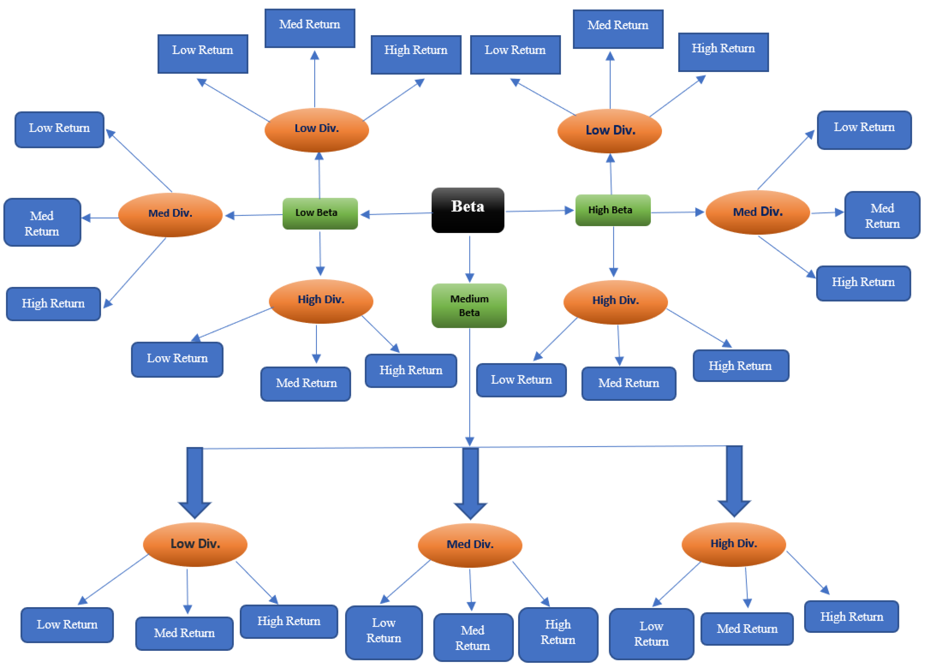
• Cluster the stocks into three groups (low, medium, and high) based on the risk factor beta.
• After we obtained the three clusters (high beta, medium beta, and low beta), each cluster was further grouped into three categories (low, medium, and high) based on the risk factor dividend yield.
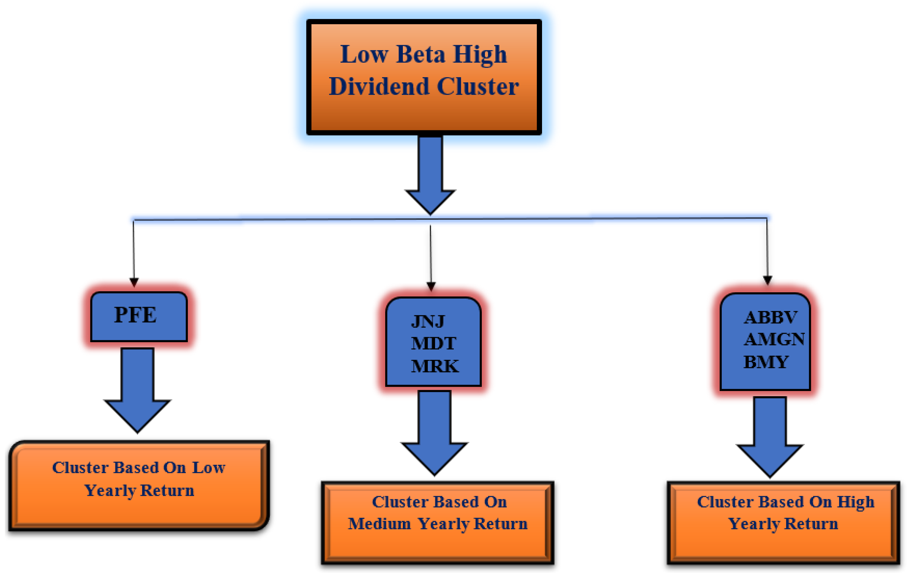
• In the final stage of clustering, we again clustered each group of dividend yield clusters based on the yearly percentage return of the stocks.

Figure 1 provides a schematic diagram of the clustering mechanism.

The above clustering mechanism produced a total of twenty-seven possible clusters to choose from. To select the appropriate stock meaningfully, we focused on the specific cluster comprised of the stocks having a low beta risk, high dividend yield, and high yearly percentage return. Figure 2 shows the stocks with these characteristics.

The above figure tells us that there were three stocks, namely ABBV, AMGN, and BMY, that matched our selection criteria. Since our goal is to build an analytical model for one stock, we chose ABBV, which had the highest dividend yield (5.4%) among the three. Also, AbbVie Inc. (ABBV) is a very popular publicly traded American biopharmaceutical company. While the company’s total revenue for 2019 grew by only 1.6%, U.S. sales of its blockbuster drug, Humira (best-selling drug in the world for several years), were up by 8.6%, and the worldwide sales of another popular drug, Imbruvica, were up more than 30%.

2.2. Description of the Indicators

After we selected ABBV as the appropriate stock, we collected information on different indicators for the stock. Our data include information from 1 August 2017 to 31 December 2019. We collected data based on three financial attributes and three economic attributes. A five-day period moving average (MA) method was used for each indicator to structure our data. One of the main goals of our study is to understand what indicators significantly affect the weekly stock price of ABBV. We used six indicators and the average weekly closing price (AWCP) as a measure of the response. A description of the attributable variables (indicators) is given below:

2.2.1. Financial Indicators

• Div_Yield ($X_1$): The dividend yield is a financial measure that demonstrates how much a company disburses in dividends each year with respect to its stock price. It is the annual dividend rate divided by the current share price. It is expressed as a percent form. For instance, if the current stock price is $\$50$ and the annual dividend is $\$1$, then the dividend yield is 2 percent.
• Beta ($X_2$): Beta is a risk measure of a stock’s volatility of return with regard to the overall market. In general, a stock with a higher beta value tends to have a higher risk and also higher expected returns. It is defined as follows:

  $$Beta={\displaystyle \frac{Cov(R_I,R_M)}{Var\left(R_M\right)}},$$

  where $R_I$ is the return on an individual stock and $R_M$ is the return on the overall market. Cov(.,.) is the covariance between $R_I$ and $R_M$, i.e., how the changes in stock return are related to the changes in the market return, Var(.) is the variance measure, implying how far the market data are scattered from their average market return.
• PE ($X_3$): The price-to-earnings ratio (P/E ratio) is the ratio that measures the current share price of a stock with respect to its earnings per share (EPS). It is defined as follows:

  $$P/ERatio={\displaystyle \frac{\mathrm{Market}\mathrm{value}\mathrm{per}\mathrm{share}}{\mathrm{Earning}\mathrm{per}\mathrm{share}}}.$$

2.2.2. Economical Indicators

• US_GDP ($X_4$): Gross domestic product of the United States (in trillions).
• US_ICS ($X_5$): The Index of Consumer Sentiment (ICS) or economic well-being was developed at the University of Michigan Survey Research Center to measure the confidence or optimism (pessimism) of consumers in their future well-being and economic conditions. The index measures the short and long-term expectations of business conditions and the individual’s perceived economic well-being. Evidence indicates that the ICS is a leading indicator of economic activity, as consumer confidence seems to pave the way for major spending decisions.
• US_PSR ($X_6$): The U.S. personal savings rate is the population’s personal savings as a percentage of their disposable personal income. In other words, it is the percentage of people’s income left after they pay taxes and spend money. The U.S. Bureau of Economic Analysis (BEA) publishes this rate.

In Figure 3, we see that the values of the response AWCP are positively skewed and do not entirely follow a Gaussian probability distribution.

A goodness-of-fit test (Shapiro–Wilk normality test, p-value = 2.265 × ${10}^{-8}$) was also performed to show that that subject data did not follow the normal probability distribution. A correlation matrix plot comprising the attributable variables is shown in Figure 4, where we see that no two variables are highly correlated, and the degree of linear association between any two variables is not high except for $Div\_Yield\left(X_1\right)$ and $log(US\_GDP)$. We also considered the US Consumer Price Index (CPI) initially in our model, but we had to drop it, as it was highly correlated with GDP (almost perfect correlation, with a correlation coefficient of 0.99).

2.3. Development of the Statistical Model

In developing a statistical model, our main goal was to express our response (AWCP) in terms of a non-linear mathematical function of all indicators with a high degree of accuracy. Thus, we proceeded to develop the statistical model, which is given by the average weekly stock price as a function of the six attributable variables (which we believe have a significant contribution to the response) and all possible interactions, as previously discussed. In the present situation, one of the pure forms of a model with all possible interactions and an additive error structure could be expressed as follows:

$$AWCP={\beta }_0+\sum _i{\alpha }_i{x}_i+\sum _j{\gamma }_j{k}_j+ϵ,$$

(1)

where ${\beta }_0$ is the intercept of the model, ${\alpha }_i$ is the coefficient of ith individual attributable variable $x_i$, ${\gamma }_j$ is the coefficient of the jth interaction term $k_j$, and $ϵ$ denotes the random disturbance or residual error of the model following a normal distribution with a zero mean and constant variance.

One of the main assumptions in constructing the above model was that the response variable AWCP should follow the Gaussian probability distribution approximately. As illustrated above, AWCP does not support the Gaussian probability distribution. Therefore, we must apply a non-linear transformation [16,17] to the response to see if the transformation can adjust the scale of the response to follow a normal probability distribution. We used a Johnson transformation [6] for our response, which results in Equation (2) below:

$$z=\gamma +\delta ln(x-ϵ),\delta >0,-\infty <\gamma <\infty ,-\infty <ϵ<\infty ,x>ϵ$$

and

$$ATWCP=-120.5+21.87ln\left(AWCP+159.83\right).$$

(2)

Here, TWCP represents the new response variable (transformed) after Johnson’s transformation has been applied. Thus, we proceeded to estimate the coefficients (weights) of the actual contributable variables for the transformed data in Equation (2). To develop our statistical model, we initially began with the full statistical model, which included all six attributable variables as previously defined and five possible interactions between each pair. Thus, at first, we started structuring our model with $\left({\displaystyle \genfrac{}{}{0pt}{}{n}{k}}\right)=15(n=6,k=2)$ potential interaction terms and six indicator terms. While we began with the full statistical model (twenty-one), as we mentioned above, we applied the process to determine the most significant contributions of both the individual attributable variables and interactions by eliminating the less-important indicators gradually. Moreover, backward elimination is deemed one of the best traditional methods for a small set of feature vectors to tackle the problem of overfitting and perform feature selection. To obtain a better accuracy, we took the log transformation of the indicators $GDP\left(X_4\right)$ to reduce its high variability. However, our statistical analysis showed that six out of the six indicators significantly contributed to the twelve interaction terms. The method eliminated three unimportant interaction terms. Thus, the best proposed statistical model with every significant indicator and interaction that accurately estimated the response AWCP were the six indicators that individually and significantly contributed and the twelve interaction terms. Hence, the best preferred statistical model with all the significantly attributable variables and interactions that estimate the weekly average stock price is given by Equation (3) below.

$$\begin{array}{cc}\hfill \widehat{TAWCP}& =\left\{\begin{array}{c}-0.083-0.12X_1-0.37X_3+5.3X_2+0.0029log\left(X_4\right)\hfill \\ +1.85X_5+6.2X_6+0.186X_1{X}_2+0.22X_1{X}_4+0.035X_1{X}_5+\hfill \\ 0.39X_1{X}_6+0.0073X_2{X}_3-0.023X_3{X}_4+0.006X_3{X}_5+\hfill \\ 0.036X_3{X}_6-0.22X_2{X}_4-0.2X_2{X}_5-0.1X_5{X}_4-0.41X_4{X}_6\hfill \end{array}\right.\hfill \end{array}$$

(3)

The TAWCP estimate is obtained using Equation (3) and is based on a Johnson transformation [6] of the data; thus, we will utilize the anti-transformation of Equation (3) to estimate the desired, actual, average weekly stock price as follows:

$$\widehat{AWCP}=-159.83+exp({\displaystyle \frac{\widehat{TAWCP}+120.5}{21.87}}).$$

(4)

The proposed model will help social researchers, economists, and financial analysts to understand how the weekly stock price varies when any one of the six attributable variables is varied, keeping the other attributable variables fixed. Similarly, the model does the same for significant interactions. Most commonly, it will estimate the conditional expectation of the response of AWCP given the indicators that are fixed at a particular level. For example, given, $X_1=4.8,X_2=0.9,X_3=31.5,X_4=22,X_5=99.4$, and $X_6=7.7$, we we obtained a predicted response value of 89.31 (from Equation (4)). Therefore, given all the values of the indicators, fixed at a particular level, the weekly average stock price for ABBV is $89.31. Furthermore, we illustrate the percentage that the indicators and the interactions contribute to the yearly percentage change in stock, and we rank them in

Table 1. Rank of the most significant indicators and their interactions according to their percent contribution to the response AWCP.

Rank	Indicators	Contribution (%)
1	$Div\_Yield$	8.95
2	$Div\_Yield\cap US\_PSR$	7.85
3	$PE\cap US\_ICS$	7.81
4	$log(US\_GDP)$	7.79
5	$US\_ICS\cap US\_GDP$	6.8
6	$US\_ICS$	6.54
7	$Div\_Yield\cap US\_ICS$	6.13
8	$PE\cap US\_PSR$	5.11
9	$BETA\cap US\_PSR$	4.76
10	$Div\_Yield\cap BETA$	4.42
11	$BETA$	4.35
12	$Div\_Yield\cap US\_GDP$	4.31
13	$BETA\cap US\_GDP$	3.75
14	$PE\cap US\_GDP$	3.67
15	$US\_PSR\cap US\_GDP$	3.37
16	$US\_PSR$	2.65
17	$PE$	2.45
18	$PE\cap BETA$	1.63

.

To assess the quality of the proposed analytical model, we use both the coefficient of determination, $R^2$, and adjusted $R^2$, which are the critical criteria to evaluate the model’s accuracy. The regression sum of squares (SSR) measures the variation that is explained by our proposed model. The sum of squared errors (SSE), also termed the residual sum of squares, is the variation that remains unexplained. We always try to minimize this error in a model, the total sum of squares (SST) = SSE + SSR. $R^2$, the coefficient of determination, is defined as the proportion of the total response variation that is explained by the the proposed model. It measures how well the regression process approximates the real data points. Thus, $R^2$ is given by

$$R^2=1-{\displaystyle \frac{SSE}{SST}}.$$

However, $R^2$ itself does not consider the number of variables in the model. Also, there is the problem of the ever-increasing $R^2$. To address these issues, we have the adjusted $R^2$ value, which considers the number of parameters and is given by

$$R_{adj}^2=1-\left[{\displaystyle \frac{(1-R^2)(n-1)}{n-k-1}}\right],$$

where n is the number of points in our data sample and k is the number of independent regressors, i.e., the number of indicators in the model, excluding the constant. For our final statistical model, the R squared is 98.89%, and the R squared adjusted is 98.85%. Both the R squared and adjusted R squared values are very high and very close to each other in our model. That is, the developed statistical model explains more than 93% of the variation in the response variable; a very high-quality model. Similarly, the indicators that we included in the the model, along with the relevant interactions, estimate more than 98% of the total variation in the response variable change. The residual standard error (RSE) represents the approximate difference between the observed and predicted outcomes in the model. We obtained an RSE value of 0.1, which implies that the observed response value differs from the predicted response value by 0.1 on average. In Table 1 below, we rank the individual attributable variables and interactions with respect to their percentage of contribution to the response AWCP.

The ranking is important, given the fact that in a survey or experiment, if the group of experimenters or surveyors know beforehand the most important variables that account for the response, then they might only collect information regarding those important variables. This will be economical and less time-consuming, as they might not be interested in the insignificant variables that contribute very little to the response or do not contribute at all. Figure 5 gives a pictorial representation of all the risk factors and interactions that significantly contribute to the response.

2.4. Residual Analysis

Once the statistical model has been developed, it is necessary to check the model assumptions by performing a residual analysis. In our case, we propose a multiple non-linear regression model, which is very useful and accurately conveys some important information regarding the subject matter.

2.4.1. Mean Residual is Approximately Zero

When one performs a multiple linear regression (or any other type of regression analysis), one obtains a line that best fits the data. Usually, all of the data points do not fall exactly on this regression equation line; they are scattered around. A residual is a vertical distance between a data point and the regression line. Each data point has one residual. The residuals are positive if they are above the regression line and negative if they are below the regression line. If the regression line perfectly passes through the point, the residual at that point is zero. The residual (error) is defined as:

$$\mathrm{residual}=\mathrm{observed}\mathrm{value}\text{-}\mathrm{predicted}\mathrm{value}=y-\widehat{y},$$

where y and $\widehat{y}$ are the observed and predicted response. $\widehat{e}$ is the estimated residual error from the linear fit. The sum of the residuals equals zero, assuming that the regression line is actually the line of “best fit”. In our case, the mean residual is $1.97\times {10}^{-18}$, implying that it is almost zero.

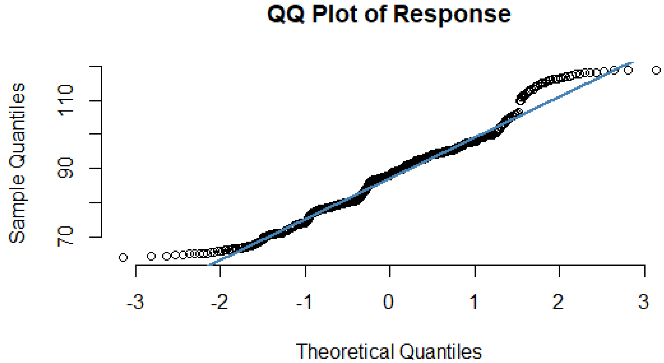
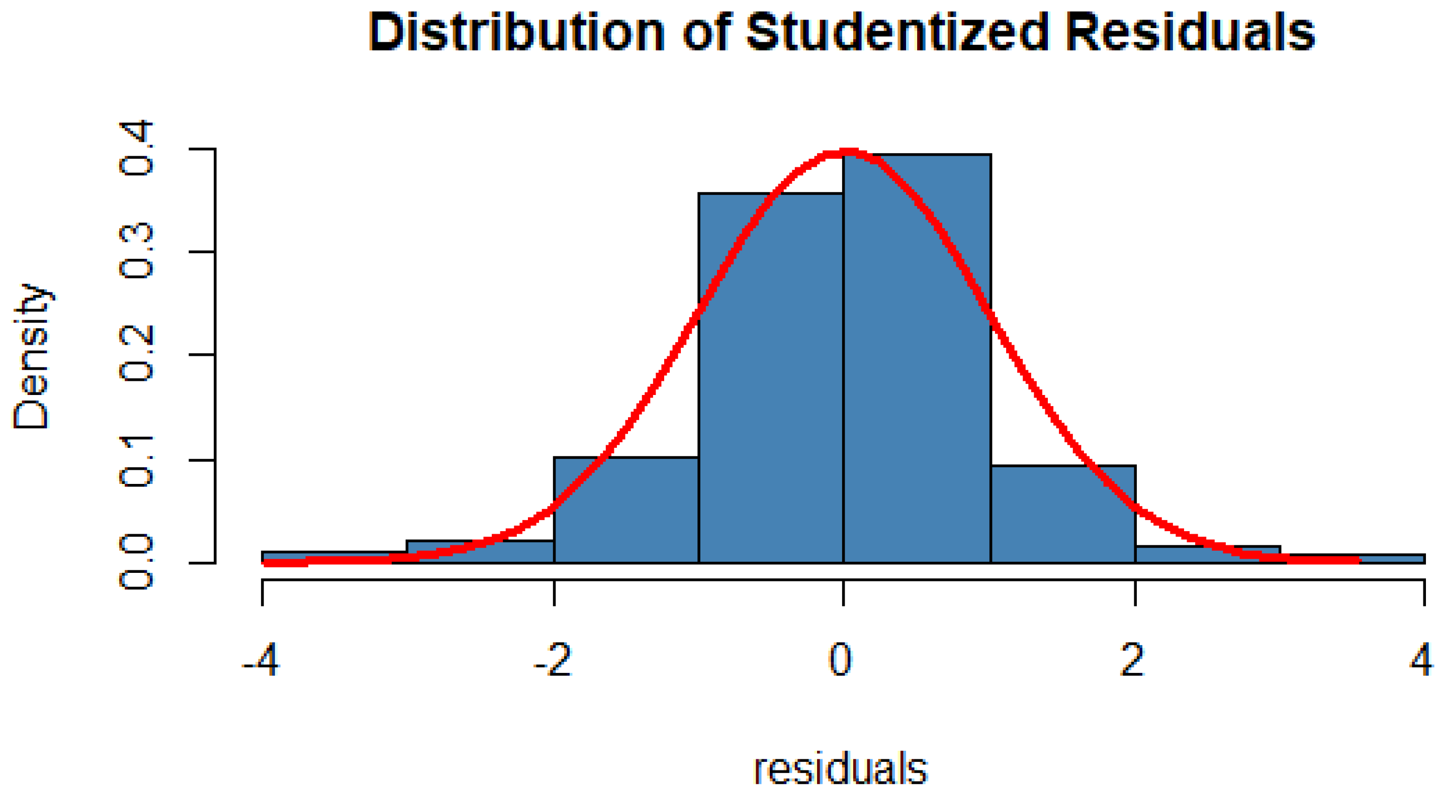
2.4.2. Normality of Residual

One of the important assumptions of the proposed model is the normality ofthe residual for the transformed response. In Figure 6, we note that the Studentized residual [15] follows a symmetric pattern.

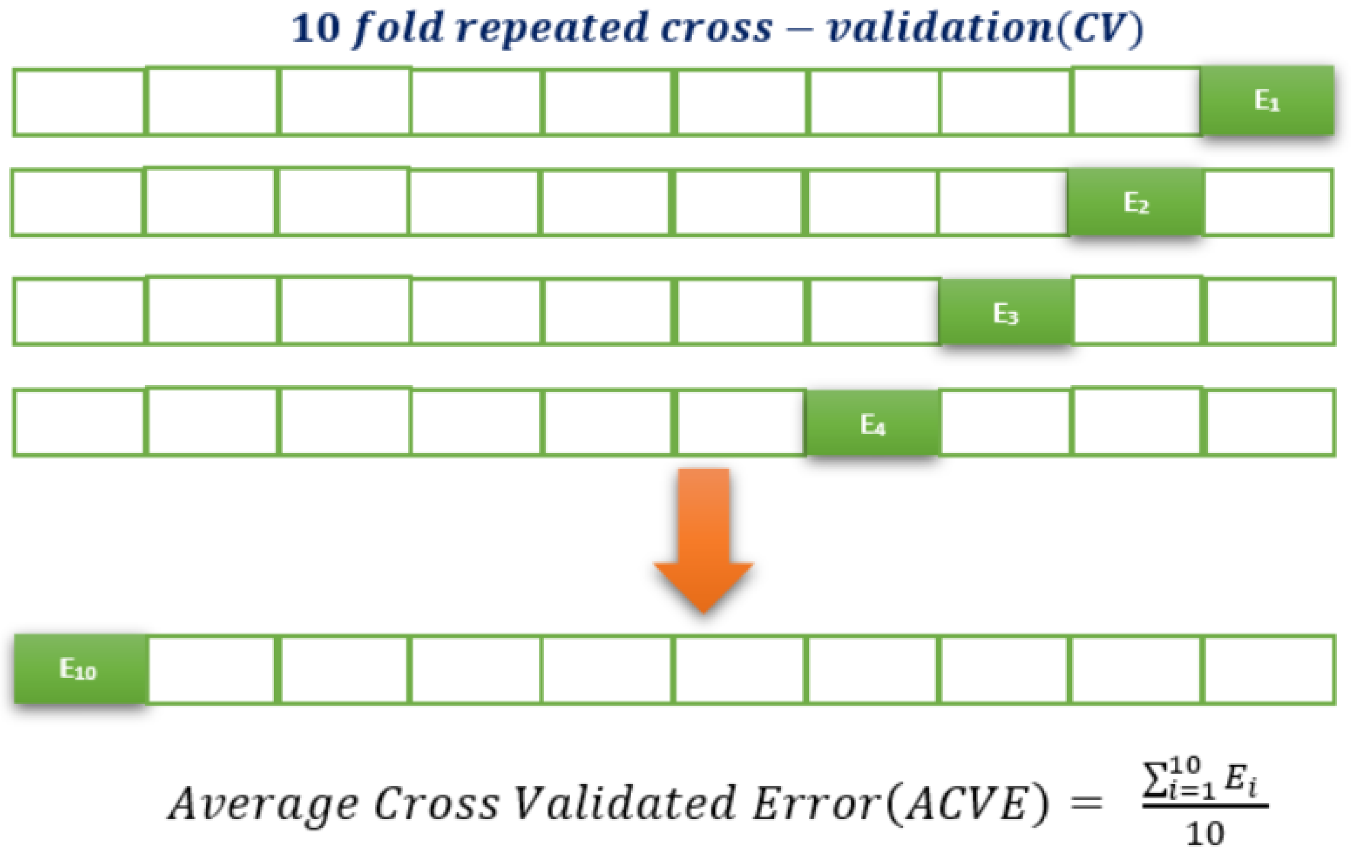
3. Validation and Prediction Accuracy of the Proposed Model

We developed our analytical model based on $80\%$ training data and validated the model based on $20\%$ testing data. In the testing data (validation data), the test error is the average error that occurs when using the analytical method to predict the response to a new observation; that is, a measurement that was not used when training the method. The test error gives an idea about the consistency of the analytical model. We obtained an accuracy of 98.7% in terms of the $R^2$ value in our validation (testing) set. Moreover, we performed repeated ten-fold cross-validation [18,19] for our validation testing. The primary objective is that we will use ten-fold cross-validation, then repeated cross-validation ten times, where each of the repetition folds is split differently. In ten-fold cross-validation, the training set is divided into ten equal subsets. One of the subsets is taken as the testing set in turn, and ($10-1$) = 9 subsets are taken as a training set in the proposed model. The mean square error $E_1$ is computed based on the held-out set. This procedure is repeated 10 times; each time, a different group of observations is treated as a validation set. This process results in 10 estimates of the test error, $E_i,i=1,\dots 10$. The average error of each set throughout the cross-validation process is termed as a cross-validated error. The following Figure 7 illustrates briefly the idea of 10-fold repeated cross-validation, where $E_i,i=1,\dots 10$ is the mean square error (MSE) in each iteration, and ACVE is the average cross-validated error.

The $R^2$, root mean square error (RMSE), and mean absolute error (MAE) for our model for the test data set are 98.7, 0.1, and 0.07, respectively. Figure 8 illustrates how the $R^2$ and $RMSE$ vary in the different folds of test data.

Figure 8 illustrates that the $R^2$ remains very high (around 98%), and the $RMSE$ remains low (around 0.1) for different repeated cross-validated folds of the test (validation) data. Hence, we can conclude that the accuracy of the model is fairly consistent. We have obtained a non-linear analytical model for ABBV’s weekly stock price with a high accuracy, which is a function of the combination of some financial and economic indicators that drive the ups and downs of this particular stock. In the next section, we will discuss some techniques that will optimize (maximize) our model response (objective function). We will also find the optimum values of all six factors that lead to the optimization of the weekly response of the ABBV stock.

4. Analytical Method to Optimize the AWCP of ABBV Inc.

A Formal Analytical Approach For the Response Surface Model Using the Desirability Function

The concept of the desirability function is one of the most frequently used methods in the industry for the optimization of one or more responses. The desirability functions approach, initially proposed by Harrington (1980) [10], is popular in the literature regarding response surface methodology (RSM). The desirability function transforms each of the estimated responses $Y_i\left(x\right)$ to a desirability value $d_i\left(Y_i\right)$, where $0\le d_i\le 1$. For an individual response $Y_i\left(x\right)$, a desirability function $d_i\left(Y_i\right)$ takes on values within [0,1]. $d_i\left(Y_i\right)=0$ represents a entirely undesirable value of response $Y_i$, and $d_i\left(Y_i\right)=1$ represents a completely desirable or ideal response value. The value of $d_i\left(Y_i\right)$ increases as the “desirability” of the corresponding response increases. The individual desirabilities are then merged using the geometric mean, which gives the overall desirability D:

$$D={\left[{\prod }_{i=1}^k{d}_i\left(Y_i\right)\right]}^{{\displaystyle \frac{1}{k}}},$$

where k denotes the number of responses. In our study, $k=1$.

Depending on whether a particular response $Y_i$ is to be maximized, minimized, or assigned a target value, different desirability functions $d_i\left(Y_i\right)$ can be used. A useful class of desirability functions was proposed by Derringer and Suich (1980) [11]. Let $L_i,U_i$, and $T_i$ be the lower, upper, and target values, respectively, that are desired for response $Y_i$, with $L_i\le T_i\le U_i$.

If there is a specific target set up for the response, then its desirability function is given by the following:

$$d_i\left(\widehat{Y_i}\right)=\left\{\begin{array}{cc}0\hfill & \mathrm{if}\widehat{Y_i}\left(x\right)<L_i\hfill \\ {\left({\displaystyle \frac{\widehat{Y_i}\left(x\right)-L_i}{T_i-L_i}}\right)}^s\hfill & \mathrm{if}{L}_i\le \widehat{Y_i}\left(x\right)\le T_i\hfill \\ {\left({\displaystyle \frac{\widehat{Y_i}\left(x\right)-U_i}{T_i-U_i}}\right)}^t\hfill & \mathrm{if}{T}_i\le \widehat{Y_i}\left(x\right)\le U_i\hfill \\ 1\hfill & \mathrm{if}\widehat{Y_i}\left(x\right)>U_i,\hfill \end{array}\right.$$

(5)

where s and t in the above equation determine how important it is to hit the target. For $t=s=1$, the desirability function increases linearly towards the direction of $T_i$. For $s<1,t<1$, the desirability function is convex, and for $s>1,t>1$, the desirability function is concave [9]. If we want the response to be maximized, the individual desirability is given as follows:

$$d_i\left(\widehat{Y_i}\right)=\left\{\begin{array}{cc}0\hfill & \mathrm{if}\widehat{Y_i}\left(x\right)<L_i\hfill \\ {\left({\displaystyle \frac{\widehat{Y_i}\left(x\right)-L_i}{T_i-L_i}}\right)}^s\hfill & \mathrm{if}{L}_i\le \widehat{Y_i}\left(x\right)\le T_i\hfill \\ 1\hfill & \mathrm{if}\widehat{Y_i}\left(x\right)>T_i,\hfill \end{array}\right.$$

(6)

where $T_i$ is interpreted as a large enough value for the response. Finally, if we want to minimize a response, the desirability function is given as follows:

$$d_i\left(\widehat{Y_i}\right)=\left\{\begin{array}{cc}1\hfill & \mathrm{if}\widehat{Y_i}\left(x\right)<T_i\hfill \\ {\left({\displaystyle \frac{\widehat{Y_i}\left(x\right)-L_i}{T_i-U_i}}\right)}^s\hfill & \mathrm{if}{T}_i\le \widehat{Y_i}\left(x\right)\le U_i\hfill \\ 0\hfill & \mathrm{if}\widehat{Y_i}\left(x\right)>U_i,\hfill \end{array}\right.$$

(7)

where $T_i$ is interpreted as a small value for the response.

The desirability function approach consists of the following steps:

• Given the data, fit response models for all k responses (in our study, we have a single response; therefore, k = 1);
• Define individual desirability functions for each response;
• Optimize the overall desirability D with respect to the controllable indicators.

5. Results

In our study, we started developing a data-driven non-linear analytical model with three financial indicators and three economic indicators. After developing the predictive model with a high accuracy, our goal is to maximize the response AWCP and find the optimum values of the indicators at which the response is being maximized. We now proceed to maximize AWCP (within its domain) in the model (4) in Section 2.3. The analytical method of optimization requires the constraints of optimization.

Table 2. Constraints on the indicators showing the lower and upper limits.

Indicators	Lower Limit	Upper Limit
Div_Yield	2.212	6.506
Beta	−0.9	2.3
PE	16.55	41.42
US_GDP	19.6	21.9
US_ICS	89.8	101.4
US_PSR	6.7	8.8

presents the constraints on the ten indicators.

Table 2 above provides the lower and upper limits of all ten indicators used in our study. Next, using Equation (6) in Section “A Formal Analytical Approach For The Response Surface Model Using Desirability Function”, we will maximize the estimated response from the model (4) and obtain the optimum values of all ten indicators.

Table 3. Estimated maximized response with optimum values of indicators.

Response and Indicators	Optimum Values
AWCP (Response)	120$
Div_Yield	4.36
Beta	0.7
PE	39.56
US_GDP	19.6
US_ICS	101.4
US_PSR	8.8

provides the estimated maximum response AWCP along with the optimum values of the indicators.

Table 4. Some useful results related to the optimized response.

Estimated Maximized Value	USD 120
Desirability	1
${\mathit{R}}^{\mathbf{2}}$	98.61%
${{\mathit{R}}^{\mathbf{2}}}_{\mathit{Adjusted}}$	98.57%
95% CI	(110.71, 129.29)
95% PI	(110.28, 129.72)

provides the values of $R^2$, ${R^2}_{Adjusted}$, and desirability along with the 95% confidence and 95% prediction interval of the estimated response WCP.

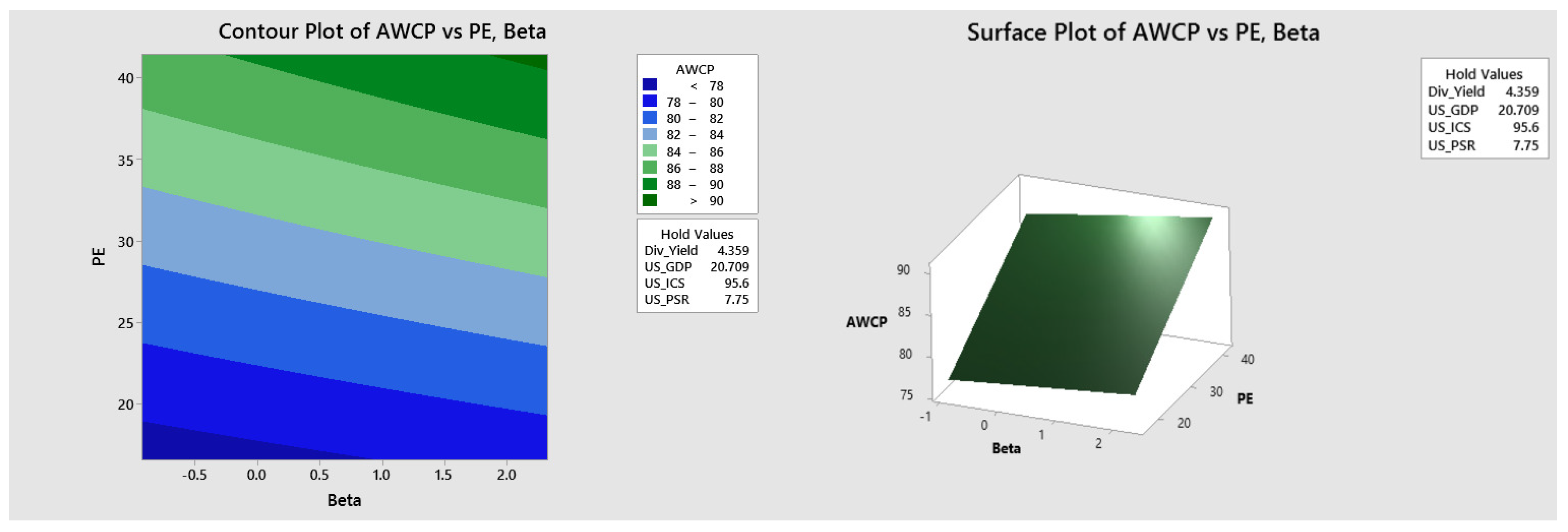
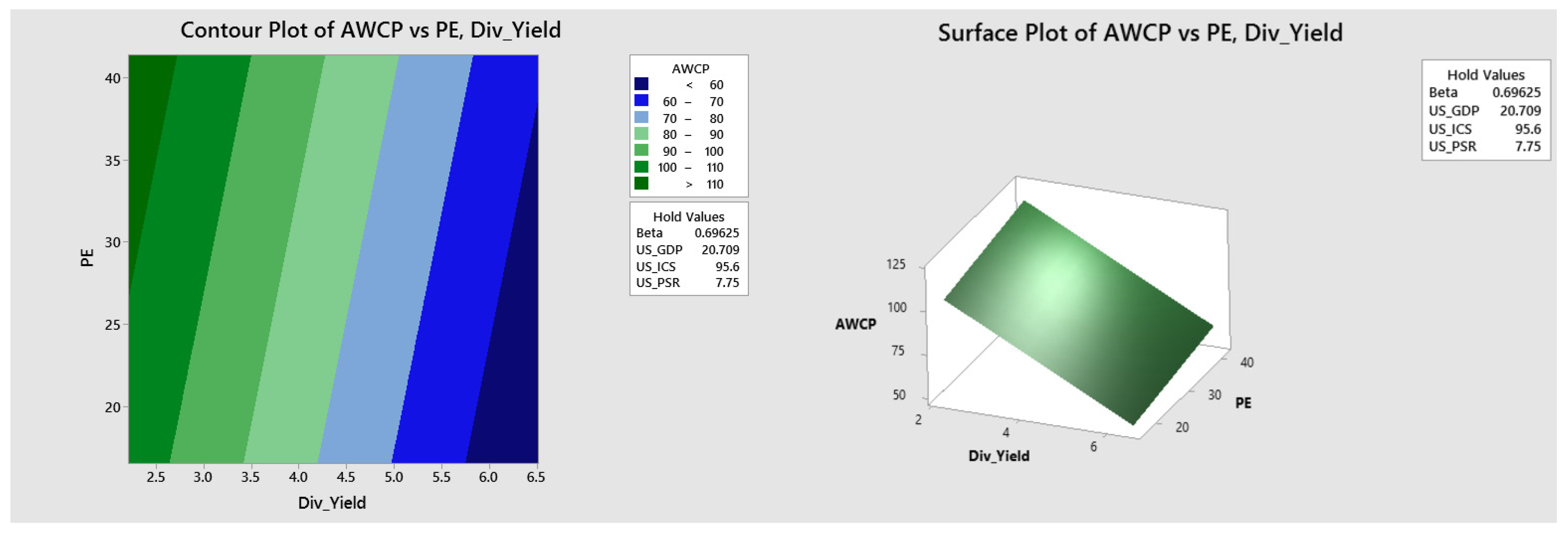
Graphical Visualization of the Estimated Response Surface

One important aspect of the response surface methodology is that it helps researchers understand variations in the response in the three-dimensional plot in the presence of any two risk factors, keeping the rest of the risk factors fixed at a particular level. Response surface plots (contour and surface plots) are very useful in order to obtain the desired values of the response and optimum conditions for any two indicators, keeping the others fixed at a particular level. In a contour plot, the response surface is observed as a two-dimensional plane, where all the points that have a similar response are connected to create contour lines of constant responses. A surface plot generally exhibits a three-dimensional view that may provide a clearer picture of the response’s behavior. Since the three economic indicators are not controllable, we will not include those plots, and we will only focus on the combination of the three financial indicators included in model (3) of Section 2.3. In this section, we will illustrate different contour and surface plots that will help researchers to understand the nature of the relationship between any of the two indicators and the response (AWCP). The following three figures (Figure 9, Figure 10 and Figure 11) describe the variation in the estimated response AWCP as any single or two indicators vary, keeping the others fixed at a particular level.

Based on Figure 9 above, we see that the estimated response is maximized (greater than 110) for any positive beta value when the dividend yield is less than approximately 2.5, keeping all other indicators at a constant level.

Based on Figure 10 above, we see that the estimated response is maximized (greater than 90) when PE is greater than approximately 40 and beta is greater than approximately 1.7, keeping all other indicators at a constant level.

Figure 11 above demonstrates that the estimated response is maximized (greater than 110) when PE is greater than approximately 17 and Div_Yield is less than approximately 2.5, keeping all other indicators constant.

6. Discussion

In this manuscript, we have developed an analytic model that describes the significant indicators and the associated interactions responsible for the ups and downs of the stock ABBV very accurately. After obtaining the significant indicators and their significant interactions, we rank them with respect to the percentage of contribution to the stock price, as shown in Figure 5. The highest contributing risk factor is $DividendYield\left(X_1\right)$, contributing 8.95% of the total variation to the response AWCP. The next most significant contribution is an interaction term, which is the combined effects of $DividendYield\left(X_1\right)$ and the US Personal Saving Rate ($X_6$), with a contribution of 7.85% to the response. Numbers 3, 4, and 5 are the combined interaction effects of $PE\cap US\_ICS(X_3\cap X_5)$, $US\_GDP\left(X_4\right)$, and the interactions between $US\_ICS\cap US\_GDP(X_5\cap X_4)$, respectively, with contributions of 7.81%, 7.79%, and 6.8%, respectively. Hence, summarizing the contributions of these indicators, we find that they explain more than 98% of the total variability in the ABBV stock price.

Table 5. List of observed and predicted values of the response AWCP.

Observations	Observed	Predicted
1	88.1	88.5
246	89.1	90.2
247	89.2	90.4
308	93.5	96.4
373	96.4	100.1
374	96.2	99
375	95	99.5
376	94	98.5
377	93	97.5
378	92.7	96
379	92.3	95
435	92	95.5
436	92	96.5
437	91.8	96.4
438	91.2	96.1
439	91.4	96.1
440	92.4	94.1
449	109.8	106
450	113.2	107.8
451	114.5	102
452	115.9	112
452	115.9	111.8
453	117	113.5
454	118.2	115.2
459	115.4	118.3
460	114.8	118.4
473	112.6	115.8
474	111.3	115.2
475	111.4	114.9
476	111.3	114.4
477	111.8	113.8
482	116.4	111
483	117.9	111
484	116.4	109.4
485	115	108.9
486	113	108.5
496	99.8	102.9
497	100	102.9
504	97.8	97.7
505	97.7	96.6
506	98	97
507	98	97

demonstrates the list of the observed and predicted responses from our data-driven non-linear analytical model. Based on Table 5, we see that the predictions using the analytical model (4) are very close to the actual observed values, testifying to our model’s high accuracy and predictive power.

Moreover, we performed a response surface analysis to maximize the estimated response of our developed analytical model, and we also obtained the optimum values for the three financial and three economic indicators. The $R^2$ and ${R^2}_{Adjusted}$ values in Table 4 attest to the fact that the optimized model is good in terms of accuracy. Also, we have obtained a similar accuracy in terms of the $R^2$ and ${R^2}_{Adjusted}$ values that we obtained using our analytical model (4). The desirability value of 1 in Table 4 indicates that the estimated fit is the most desirable/ideal. We can address the usefulness and importance of the proposed model in the subject area as follows:

• We identified and tested the individual attributable variables (indicators) responsible for the increases or decreases in the ABBV stock price.
• The significant interactions that influence the response AWCP in our model were identified.
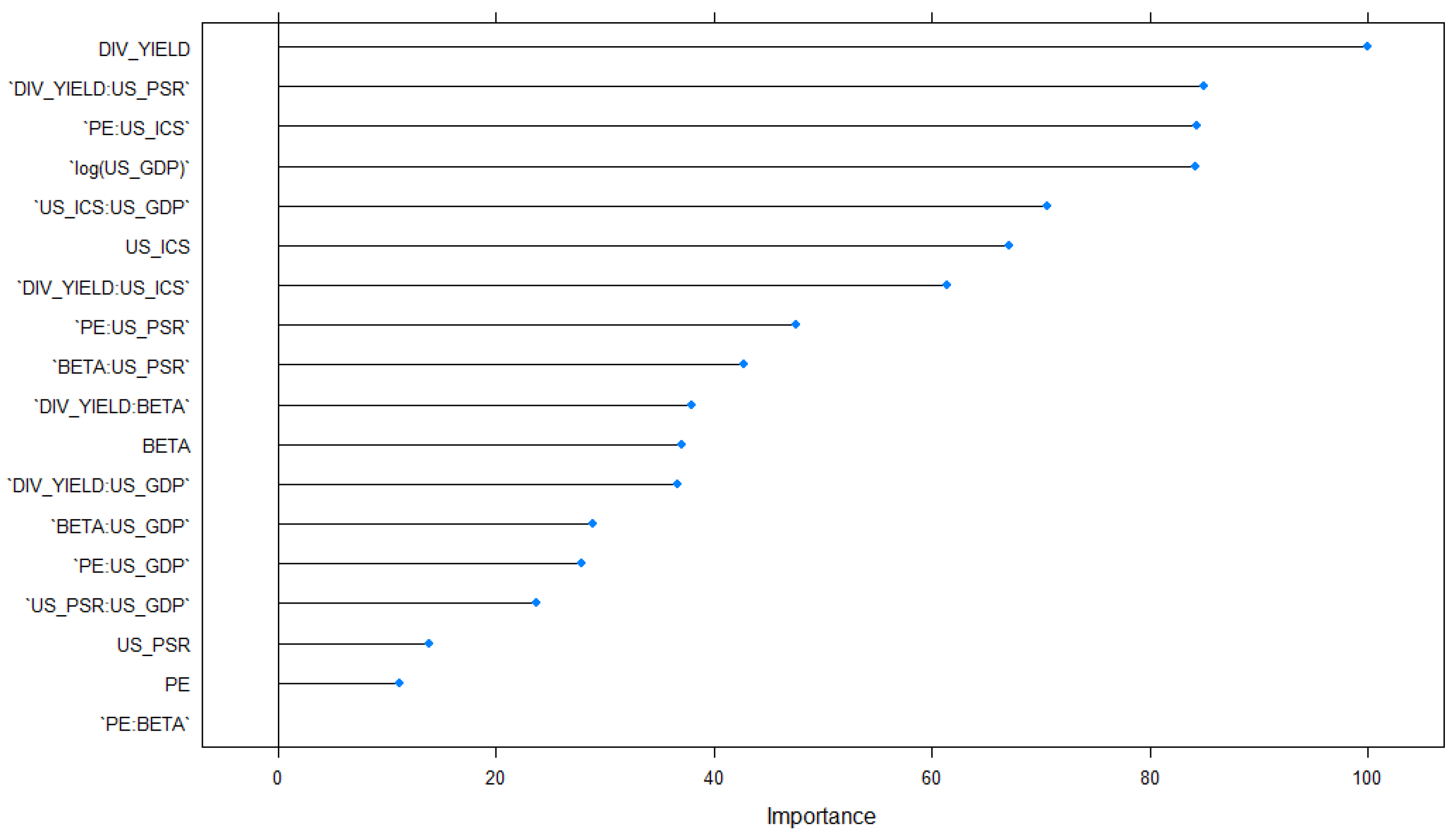
• The individual attributable indicators and interactions were ranked with respect to the percentage of contribution to the response.
• Excellent predictions of the weekly closing price for the healthcare stock ABBV from our analytical model can be obtained with a high degree of prediction accuracy.
• We compared the original and the estimated response AWCP using our analytical model and found that they are very close to each other, indicating the high accuracy of our model.
• A desirability function approach was performed for this stock, ABBV Inc., to maximize the predicted response based on the average weekly closing price (AWCP). We also identified the optimum levels of the indicators that maximized the predicted response with a high degree, along with the 95% confidence interval and 95% prediction interval.

7. Conclusions

As the investment landscape continues to evolve, the requirement for robust and reliable stock prediction models has become increasingly imperative for both investors and financial analysts. One of the main goals of this study was to investigate the practical and policy implications of analytical models that utilize beta risk, dividend yield, and price-to-earnings ratio as predictors of stock performance [20]. The consideration of beta risk as one of the predictors in stock prediction models holds important implications for investors. Empirical research indicates that low-beta stocks tend to generate higher returns, as their beta values positively covary with market variance and the stochastic discount factor [21,22]. This phenomenon, known as the “betting against beta” anomaly, challenges the traditional security market line and underscores the significance of accounting for time-varying risk premiums in asset pricing models [23]. For financial analysts, accurately modeling the impact of beta risk on expected returns can enhance the accuracy of their forecasts and provide valuable insights to support informed investment decision-making. Additionally, the incorporation of dividend yield as a predictor in stock forecasting models carries significant policy implications. Existing research has demonstrated that a firm’s current investment decisions, dividend payouts, and return on capital have a substantial influence on the likelihood of future dividend changes, as do the variance and persistence of shocks to capital productivity [24,25]. These findings suggest that policymakers should carefully evaluate the impact of regulatory changes on corporate-level dividend policies, as such policies can have wide-ranging consequences for investor conduct and overall market stability. The developed analytical model was evaluated using several statistical methods including, the $R^2$ and $R_{adjusted}^2$ values, which attest to its high quality.

Investment bankers and financial analysts usually keep track of a company’s stock price and percentage increase in stock price to measure a company’s financial solvency, market performance, and general viability. A steadily rising stock price indicates that a company is moving in the direction of money-making. Additionally, if the stockholders are happy and the company is on its way towards prosperity, the executives are likely to retain their positions within the company. Conversely, if a company is struggling, as reflected by a deteriorating stock price, a company’s board of directors may decide to dismiss its top operatives. Thus, decreasing stock prices are not good for a company’s higher-ups and financial health as a whole. Our study’s findings suggest that financial analysts and quantitative researchers might need to pay more attention to different significant financial and economic attributes, as our research suggests, that will maximize the stock price. Following the same manner, this specific stock was selected based on its low beta risk, high dividend, and high yearly % yield from the healthcare business sector (HBS) of the S&P 500. An individual stock or a cluster of stocks can be selected from any of the other ten business segments (information technology, financial sector, real estate, consumer discretionary, communication services, industrial sector, consumer staples, energy, utilities, and materials) of the S&P 500. The same analytical procedure for stock selection can be implemented to any sector of the S&P 500 cumulatively or an individual stock specific to a sector. Financial analysts can build a similar model based on other stocks, depending on the research interest. Also, since the individual ups and downs of the stock price of an organization have a positive correlation with current and future increases in the productivity growth rate per business cycle, our proposed statistical model can be used for firms’ promotion policies, and they may be useful for managers and human resource professionals. Financial analysts can use our model to predict the individual company’s percentage change in stock price by using significant indicators. This will help the different financial firms to identify their financial health, as the higher a stock price is, the more likely a company’s prospects become. Identifying those financial institutions is essential, as the increased stock price is correlated with an increase in productivity. Finally, our proposed statistical model is highly useful for decision making and strategic planning for controlling the factors responsible for the company’s long-term viability.

References

1. Lajevardi, S. A study on the effect of P/E and PEG ratios on stock returns: Evidence from Tehran Stock Exchange. Manag. Sci. Lett. 2014, 4, 1401–1410. [Google Scholar] [CrossRef]
2. Lemmon, M.; Portniaguina, E. Consumer confidence and asset prices: Some empirical evidence. Rev. Financ. Stud. 2006, 19, 1499–1529. [Google Scholar] [CrossRef]
3. Tang, G.Y.N.; Shum, W.C. The conditional relationship between beta and returns: Recent evidence from international stock markets. Int. Bus. Rev. 2003, 12, 109–126. [Google Scholar] [CrossRef]
4. Garner, C.A. Should the decline in Personal Saving Rate Be a Cause of Concern? Econ. Rev. Quart. 2006, 91, 5–28. [Google Scholar]
5. Avouyi-Dovi, S.; Matheron, J. Productivity and stock prices. Banq. Fr. Financ. Stab. Rev. 2006, 81–94. [Google Scholar]
6. Polansky, A.M.; Chou, Y.-M.; Mason, R.L. An algorithm for fitting Johnson transformations to non-normal data. J. Qual. Technol. 1999, 31, 345–350. [Google Scholar] [CrossRef]
7. Myers, R.H.; Montgomery, D.C.; Anderson-Cook, C.M. Response Surface Methodology: Process and Product Optimization Using Designed Experiments; John Wiley & Sons: Hoboken, NJ, USA, 2016. [Google Scholar]
8. Harrington, E.C. The desirability function. Ind. Qual. Control. 1965, 21, 494–498. [Google Scholar]
9. Derringer, G.; Suich, R. Simultaneous optimization of several response variables. J. Qual. Technol. 1980, 12, 214–219. [Google Scholar] [CrossRef]
10. Chakraborty, A.; Tsokos, C.P. An AI-driven Predictive Model for Pancreatic Cancer Patients Using Extreme Gradient Boosting. J. Stat. Theory Appl. 2023, 22, 262–282. [Google Scholar] [CrossRef]
11. Chakraborty, A.; Tsokos, C.P. A Modern Analytical Approach for Assessing the Treatment Effectiveness of Pancreatic Adenocarcinoma Patients Belonging to Different Demographics and Cancer Stages. J. Cancer Res. Treat. 2023, 11, 13–18. [Google Scholar] [CrossRef]
12. Chakraborty, A.; Tsokos, C.P. A real data-driven clustering approach for countries based on happiness score. Amfiteatru Econ. 2021, 23, 1031–1045. [Google Scholar] [CrossRef]
13. Chakraborty, A.; Tsokos, C.P. A Real Data-Driven Analytical Model to Predict Happiness. Sch. J. Phys. Math. Stat. 2021, 3, 45–61. [Google Scholar] [CrossRef]
14. Chakraborty, A.; Tsokos, C.P. Survival Analysis for Pancreatic Cancer Patients Using Cox-Proportional Hazard (CPH) Model. Glob. J. Med. Res. 2021, 21, 29–46. [Google Scholar] [CrossRef]
15. Gray, J.B.; Woodall, W.H. The maximum size of standardized and internally studentized residuals in regression analysis. Am. Stat. 1994, 48, 111–113. [Google Scholar] [CrossRef]
16. Pek, J.; Wong, O.; Wong, A.C.M. How to address non-normality: A taxonomy of approaches, reviewed, and illustrated. Front. Psychol. 2018, 9, 2104. [Google Scholar] [CrossRef] [PubMed]
17. Lee, D.K. Data transformation: A focus on the interpretation. Korean J. Anesthesiol. 2020, 73, 503. [Google Scholar] [CrossRef] [PubMed]
18. Fushiki, T. Estimation of prediction error by using K-fold cross-validation. Stat. Comput. 2011, 21, 137–146. [Google Scholar] [CrossRef]
19. Dor, O.; Zhou, Y. Achieving 80% ten-fold cross-validated accuracy for secondary structure prediction by large-scale training. Proteins Struct. Funct. Bioinform. 2007, 66, 838–845. [Google Scholar] [CrossRef] [PubMed]
20. Enke, D.; Thawornwong, S. The use of data mining and neural networks for forecasting stock market returns. Expert Syst. Appl. 2005, 29, 927–940. [Google Scholar] [CrossRef]
21. Boloorforoosh, A.; Christoffersen, P.; Fournier, M.; Gouriéroux, C. Beta risk in the cross-section of equities. Rev. Financ. Stud. 2020, 33, 4318–4366. [Google Scholar] [CrossRef]
22. Campbell, J.Y.; Vuolteenaho, T. Bad beta, good beta. Am. Econ. Rev. 2004, 94, 1249–1275. [Google Scholar] [CrossRef]
23. Ferson, W.E.; Harvey, C.R. The variation of economic risk premiums. J. Political Econ. 1991, 99, 385–415. [Google Scholar] [CrossRef]
24. Black, F.; Scholes, M. The effects of dividend yield and dividend policy on common stock prices and returns. J. Financ. Econ. 1974, 1, 1–22. [Google Scholar] [CrossRef]
25. Cyert, R.; Kang, S.-H.; Kumar, P. Managerial objectives and firm dividend policy: A behavioral theory and empirical evidence. J. Econ. Behav. Organ. 1996, 31, 157–174. [Google Scholar] [CrossRef]
Figure 1. Schematic diagram of stock clustering mechanism.
Mathematics 12 02407 g001
Figure 2. Stocks with a low beta risk, high dividend yield, and high yearly percentage return.
Mathematics 12 02407 g002
Figure 3. Q-Q Plot of the response WCP.
Mathematics 12 02407 g003
Figure 4. Correlation matrix of the indicators.
Mathematics 12 02407 g004
Figure 5. Importance plot of the risk factors and interactions according to their contributions to the response.
Mathematics 12 02407 g005
Figure 6. Normality of Studentized residual plot.
Mathematics 12 02407 g006
Figure 7. Brief Illustration of repeated ten-fold cross validation.
Mathematics 12 02407 g007
Figure 8. Variation in R 2 and R M S E in different folds.
Mathematics 12 02407 g008
Figure 9. Contour plot (left) and surface plot (right) of the estimated response surface as Div_Yield and beta vary, keeping other indicators fixed at a specified level.
Mathematics 12 02407 g009
Figure 10. Contour plot (left) and surface plot (right) of the estimated response surface as PE and beta vary, keeping other indicators fixed at a specified level.
Mathematics 12 02407 g010
Figure 11. Contour plot (left) and surface plot (right) of the estimated response surface as PE and Div_Yield kary, keeping other indicators fixed at a specified level.
Mathematics 12 02407 g011