Abstract
With increasing wafer sizes and diversifying die patterns, automated optical inspection (AOI) is progressively replacing traditional visual inspection (VI) for wafer defect detection. Yet, the defect classification efficacy of current AOI systems in our case company is not optimal. This limitation is due to the algorithms’ reliance on expertly designed features, reducing adaptability across various product models. Additionally, the limited time available for operators to annotate defect samples restricts learning potential. Our study introduces a novel hybrid self-training algorithm, leveraging semi-supervised learning that integrates pseudo-labeling, noisy student, curriculum labeling, and the Taguchi method. This approach enables classifiers to autonomously integrate information from unlabeled data, bypassing the need for feature extraction, even with scarcely labeled data. Our experiments on a small-scale set show that with 25% and 50% labeled data, the method achieves over 92% accuracy. Remarkably, with only 10% labeled data, our hybrid method surpasses the supervised DenseNet classifier by over 20%, achieving more than 82% accuracy. On a large-scale set, the hybrid method consistently outperforms other approaches, achieving up to 88.75%, 86.31%, and 83.61% accuracy with 50%, 25%, and 10% labeled data. Further experiments confirm our method’s consistent superiority, highlighting its potential for high classification accuracy in limited-data scenarios.
MSC:
68Txx
1. Introduction
Wafers are crucial in integrated circuit (IC) manufacturing and hold a significant position in the electronics industry. Taiwan’s expertise in wafer technology is a key component of the global semiconductor supply chain. In 2021, Taiwan accounted for 26% of the global semiconductor market share, ranking second worldwide. It is also expected to control 44% of the global wafer foundry capacity by 2025. Taiwan’s contributions to IC design and packaging are notable, with substantial market shares globally. In response to its strategic importance, Taiwan is expanding its wafer fabrication facilities to countries including the USA, China, Japan, and Singapore.
The semiconductor industry’s upstream segment includes companies specializing in IC design and silicon wafer manufacturing. Midstream manufacturers’ main task is to transfer the circuit designs from IC design firms onto the silicon wafers produced by manufacturers. After fabrication, these wafers are dispatched to downstream packaging and testing facilities. Quality assurance mandates die defect inspections before packaging. Initially, the case company predominantly used visual inspection (VI), which is prone to human error and inconsistent defect judgment, particularly with inexperienced inspectors. To mitigate these issues, the company has adopted automated optical inspection (AOI) as the primary inspection method. AOI machines typically utilize the golden template matching technique to discern differences between the die and a standard template, identifying defects effectively.
Although current AOI machines proficiently identify defective die patches, their defect classification algorithms demand significant customization. These algorithms depend on intricately designed features by experts, tailored for each specific application. With the ongoing evolution in wafer manufacturing, marked by increasing wafer sizes and more complex die patterns, and the variable conditions under which patches are captured, the existing algorithms lack the flexibility for universal application across different product models. Current AOI machines face limitations in defect classification efficacy due to their reliance on expertly designed features, which reduces adaptability across various product models. Additionally, the time constraints on operators for annotating defect samples restrict the learning potential of these systems. These challenges call for an innovative approach that can enhance defect classification accuracy while minimizing the need for extensive manual data annotation. Consequently, this study aims to adopt a self-training approach from semi-supervised learning (SSL) to refine die defect classification in AOI systems. Key contributions include:
- Development of an SSL that integrates pseudo-labeling, noisy student techniques, curriculum learning, and the Taguchi method.
- Creation of an adaptive system capable of autonomously integrating information from unlabeled data, bypassing the need for extensive feature extraction.
- Application of the Taguchi method for optimizing modeling strategies will diminish the manual annotation burden and save valuable time that would be needed for extensive data labeling prior to modeling.
- This method is notable for its capacity to autonomously update the classifier’s parameters with minimal labeled data while integrating unlabeled data, thus boosting the classifier’s efficacy and adaptability. Empirical validation of the proposed method’s superiority over supervised learning approaches, particularly in scenarios with scarce labeled data.
The paper is organized into five sections: The first section introduces the study, outlining its background, motivation, and objectives, and provides an overview of the current demand for IC and the state of die inspection in AOI systems. The second section reviews literature on advancements in die defect inspection and SSL methodologies. The third section details the research methodology, including the hardware architecture, proposed algorithms, and evaluation metrics for classification performance. The fourth section presents the experimental analysis, assessing the effectiveness of the proposed methods across different data annotation scenarios and their comparison with existing algorithms. The concluding section summarizes the findings and implications of the research.
2. Literature Review
This section offers a review of die inspection methodologies historically employed in the semiconductor industry, followed by an examination of SSL models in contexts with limited labeled data.
2.1. Literature on Die Defect Inspection
Advancements in 5G, IoT, and related sectors have increased the need for efficient wafer inspection methods. Techniques like design-rule checking, golden template matching, machine learning, and deep learning are used to automate die inspection in IC manufacturing.
- Design-rule checking, also known as the knowledge database method, identifies and catalogs geometric and texture features on dies, as shown by [1,2]. However, the variability in die images makes defect detection challenging with this method.
- Golden template matching, also known as the image-to-image reference method, involves comparing a golden template with the inspected image to identify potential defects based on significant differences. Chou et al. employed this method to highlight and classify defects by measuring size, shape, position, and color [3]. Zhang et al. segmented pads and die boundaries to determine defect types based on location, object count, and area [4]. Alignment between the inspected image and the golden template is crucial for accurate subtraction. To address alignment issues, Guan et al. introduced a golden template self-generating method using repetitive wafer patterns [5]. Liu et al. employed discrete wavelet transform (DWT) to extract a standard image from defective IC chip images, highlighting defects through differences and mitigating brightness variations [6]. Li et al. proposed an automatic alignment method for wafer positioning based on the standard samples, effective for measuring multiple targets [7]. Despite avoiding calibration issues, these methods require extended focal lengths for structural pattern capture, making minute defect detection challenging at lower resolutions.
- Machine learning techniques adjust model weights to map die features to defect classes. Su et al. used average grayscale values from segmented die images to train models with backpropagation neural network (BPNN), radial basis function neural network (RBFNN), and learning vector quantization neural network (LVQNN) [8]. Chang et al. used k-means clustering to distinguish areas in LED dies and extracted geometric and texture features for defect identification with LVQNN [9]. Timm and Barth measured the discontinuity around the p-electrode of LED dies using radially encoded features and a one-class support vector machine (OSVM) for high accuracy [10]. Jizat et al. developed die defect classifiers, with logistic regression achieving 86.0% accuracy [11]. Machine learning methods require distinct feature sets for different die images, making the process time-consuming.
- Deep learning adjusts model weights to automatically learn the relationship between die features and defect classes. Cheon et al. used a 4-layer CNN for classifying five types of die defects and employed k-NN in a 3D autoencoder space for unknown defects [12]. Lin et al. designed a 6-layer CNN for LED die defect classification and used CAM for defect localization [13]. Chen et al. created a CNN with convolution, separable convolution, and bottleneck layers for four defect types, utilizing generating adversarial networks (GAN) for data augmentation [14]. Saqlain et al. introduced an ensemble classifier for wafer map defects, improving defect identification efficiency by dividing the wafer into regions and removing noise [15]. Chen et al. combined GAN and YOLOv3 for die defect detection, requiring fewer defective samples and annotations, which is beneficial for diverse die patterns [16].
From the developmental context of the aforementioned literature, it is evident that rule-based and machine learning methods necessitate extensive feature engineering. Any detection algorithms related to feature extraction must be adjusted with changes in product models. The golden template method requires precise calibration for implementation, and a stable environment must be maintained during the imaging process to avoid interference. Only deep learning-related methods eliminate the need for any feature extraction process and possess the capability to counteract exceptions such as shifts, rotations, and exposures. The remarkable abilities of deep learning have attracted worldwide attention, which motivates the focus of this study on methods related to deep learning.
2.2. Literature on Semi-Supervised Learning
SSL is a method that falls between supervised and unsupervised learning. It enhances the learning capability of models by utilizing both labeled and unlabeled data for training. SSL algorithms offer a means to explore potentially useful information within unlabeled data, mitigating the need for extensive data labeling and, thus, reducing the time and manpower required for this task. In essence, SSL holds the potential to enhance learning performance even when only a small amount of labeled data is available.
SSL can broadly be categorized into deep generative, consistency regularization, graph-based regularization, and self-training [17], each of which is described below:
- Deep generative. This approach employs deep neural networks for data generation, applicable to various types of data, including images, audio, and text. Unlike traditional generative models, deep generative models can capture the intricate details of data, such as textures or contours in image data, and progressively learn higher-level features like object shapes and poses, thereby generating more realistic and diverse data. Gordon et al. used a variational autoencoder (VAE) to generate images similar to the original ones by capturing their structural elements [18]. They applied this approach to two datasets: handwritten digit recognition and clothing recognition. Through experiments with different quantities of labeled data, they found that, in the clothing dataset, having only 500 labeled data points outperformed 3000 labeled ones, with an accuracy exceeding 4.36%. In conducting experiments with varying amounts of labeled data, the authors noted that more labeled data does not necessarily correlate with increased accuracy. Zhang et al. employed the VAE method for bearing defect identification across 10 classes [19]. In experiments using varying quantities of labeled data, with the smallest being 0.25% and the largest being 50% of the total data, an accuracy exceeding 7% compared to CNN and Autoencoder was achieved with just 2.5% labeled data, while only a 4% increase was noted with 50% labeled data. The authors highlighted that incorrect labeling could impair the performance of supervised learning, and adopting deep generative models to abstain from labeling uncertain data is an effective solution to this issue.
- Consistency regularization. This approach enhances the model’s generalization ability by ensuring similar outputs under different inputs. This method is particularly beneficial in semi-supervised learning scenarios, where a small portion of the data is labeled and the majority remains unlabeled. The model makes two predictions for the unlabeled data—initially for the original data and secondly for a slightly perturbed version of the same data points. Perturbations can be introduced through random rotations, scaling, or adding noise. Chen et al. introduced a method for the classification of hyperspectral images, utilizing deep representation feature learning (DRFL) and virtual adversarial training (VAT) [20]. DRFL aids in learning representative features from the data that enhance classification accuracy, while VAT regularizes the data to benefit the prediction distribution of the training data. This approach, advantageous in utilizing unlabeled data, not only boosts accuracy but also saves annotation time. With only 0.1% of the data labeled, accuracy rates of 90.45%, 93.31%, and 94.56% were achieved on three public datasets, respectively. Noroozi et al. presented VAT, evaluated across multiple validation tasks, enhancing generalization ability and mitigating overfitting through input perturbations using VAT on unlabeled data [21]. Experiments on three public datasets, with unlabeled data proportions of 0.01%, 0.16%, 37%, and all, consistently outperformed traditional supervised learning methods. However, performance was not proportionally better with fewer labeled data compared to more.
- Graph-based regularization. This method involves smoothing the graphical structural data in images to eliminate noise. It perceives an image as a graph composed of pixels and their interconnections and employs the graph’s smoothing property for regularization. These connections can be spatial relationships between pixels or similarities in attributes like brightness or color. Liao et al. proposed a transformer fault diagnosis method using a graph convolutional network (GCN) that employs a minimal amount of unlabeled data to fully represent the similarity between labeled and unlabeled data [22]. This is a significant improvement over traditional methods that rely on trained models to determine the relationships between data. The experimental results showed that the GCN outperformed CNN, BPNN, XGBoost, and SVM in terms of accuracy.
- Self-training. Self-training involves using a model to make predictions on unlabeled data, adopting the high-confidence predicted labels as true labels to expand the labeled dataset, thereby enhancing the model’s performance. The initial training is performed on labeled data; then, the model is used to make predictions, obtaining some predicted labels. Unlabeled data with predictions exceeding a certain confidence threshold are then added to the training dataset. The model is retrained, and this process is repeated until the model converges or meets the predetermined stopping criteria. Do et al. introduced a pseudo-labeling technique grounded in the challenges of insufficient labeled data and data imbalance [23]. This method leverages both a small amount of labeled data and a large volume of unlabeled data to address the imbalance. When applied to wafer maps, the experimental results demonstrated that this method enhanced classification accuracy to 77.26%, a 6.07% improvement over traditional methods, even with the use of relatively fewer labeled data. Zhuo et al. noted the advancement in technology that has led to the development of nanoscale dies within wafers [24]. These dies are not visible to the naked eye, and computer vision technology is utilized to identify minor defects. In scenarios of scarcely labeled data and class imbalance, the SSL pseudo-labeling method offers a resolution. With less than 10% of labeled data, this approach achieved results comparable to a fully labeled (100%) dataset and outperformed existing advanced methods, reaching an average precision of 93%. Kahng et al. advocated that pseudo-labeling is highly effective for wafer defect detection, yielding impressive results even with limited labeled data [25]. Different volumes of labeled data, namely, 1%, 5%, 10%, 25%, 50%, and 100%, resulted in classification accuracies of 71.8%, 82.3%, 84.5%, 86.4%, 88.6%, and 88.0%, respectively. Interestingly, fully labeled (100%) data did not significantly enhance classification accuracy, underscoring that appropriate data augmentation is pivotal in controlling model performance. Inappropriate data augmentation can inadvertently eliminate valuable information. Liu and Ye introduced the noisy student method for tile surface defect classification, a semi-supervised learning approach [26]. Compared to traditional supervised learning, this method utilizes unlabeled data to reduce annotation costs, and experimental results revealed a defect classification accuracy of 90.13%, even with just 4.4% of the data labeled. Wang et al. developed the curriculum labeling method for semi-supervised human keypoint localization problems [27]. This iterative pseudo-labeling technique assigns labels to unlabeled image data, alternating training between labeled data and pseudo-labeled data. The authors also introduced reinforced learning to automatically learn the optimal curriculum, further enhancing localization accuracy. Kim et al. developed an automatic defect classification system for wafer surfaces using semi-supervised learning with defect localization. Their approach significantly reduces labor by improving classification accuracy by 12.56% compared to supervised models. The system effectively utilizes a combination of a small set of labeled data and a larger pool of unlabeled images, enhancing the robustness and efficiency of defect management processes [28]. Qiao et al. developed DeepSEM-Net, leveraging a dual-branch CNN-transformer architecture for semiconductor defect analysis. Their method uses a self-training, semi-supervised system, reducing manual inspection. It achieved a classification accuracy of 97.25% and a segmentation IoU of 84.40%, demonstrating substantial effectiveness on diverse datasets [29].
Compared to the potential complexity and substantial computational resources required to train deep generative models, self-training offers a simpler training process and lower computational costs. Unlike consistency regularization, which may underperform with significant input distribution variations or noise, self-training is not constrained by such limitations. Graph-based regularization methods require effective graph structure establishment and utilization and may face computational efficiency issues with small datasets. In contrast, self-training avoids such complex data processing, motivating this study’s focus on self-training.
3. Research Methods
This section introduces the hardware structure used for AOI, the hybrid self-training algorithm developed in this study, and the metrics used to evaluate the algorithm’s performance.
3.1. Description of Hardware Structure
To obtain images of the die surfaces on the wafer, this study utilizes the imaging mechanism illustrated in Figure 1 to capture shots of the die blocks. The machine employs a charge-coupled device (CCD) to take color images with a resolution of 720 × 720 × 3. A front-lit ring light source is paired with it to enhance the surface features of the items under inspection. During the capturing process, an XY axis motion controller follows an S-shaped scanning path to photograph each area of the dies that are awaiting inspection.
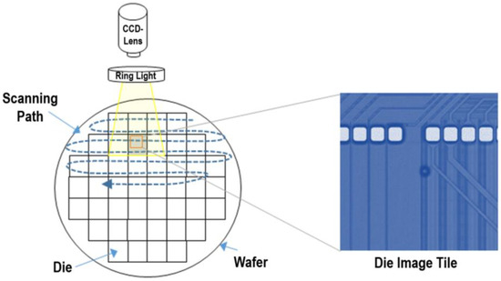
Figure 1.
Schematic diagram of AOI die defect detection.
As illustrated in Figure 1, the structure of a die comprises the pad, ion implantation zone, and bottom layer. The pad serves primarily for electrical testing, verifying the die’s functionality. In the ion implantation zone, ions are accelerated by an electric field and integrated into the die at high energies. The bottom layer acts as a protective thin-film barrier, shielding the components from chemical reactions, moisture, corrosion, and contamination.
During the wafer’s manufacturing process, the die surface might be contaminated due to residual dust particles or suffer from scratches and etching, leading to surface defects. These micro-defects appear at random; traces of them can potentially be found across the entire surface of the dies, showcasing a variety of shapes. At times, they can even appear in closely packed clusters.
3.2. Hybrid Self-Training Algorithm
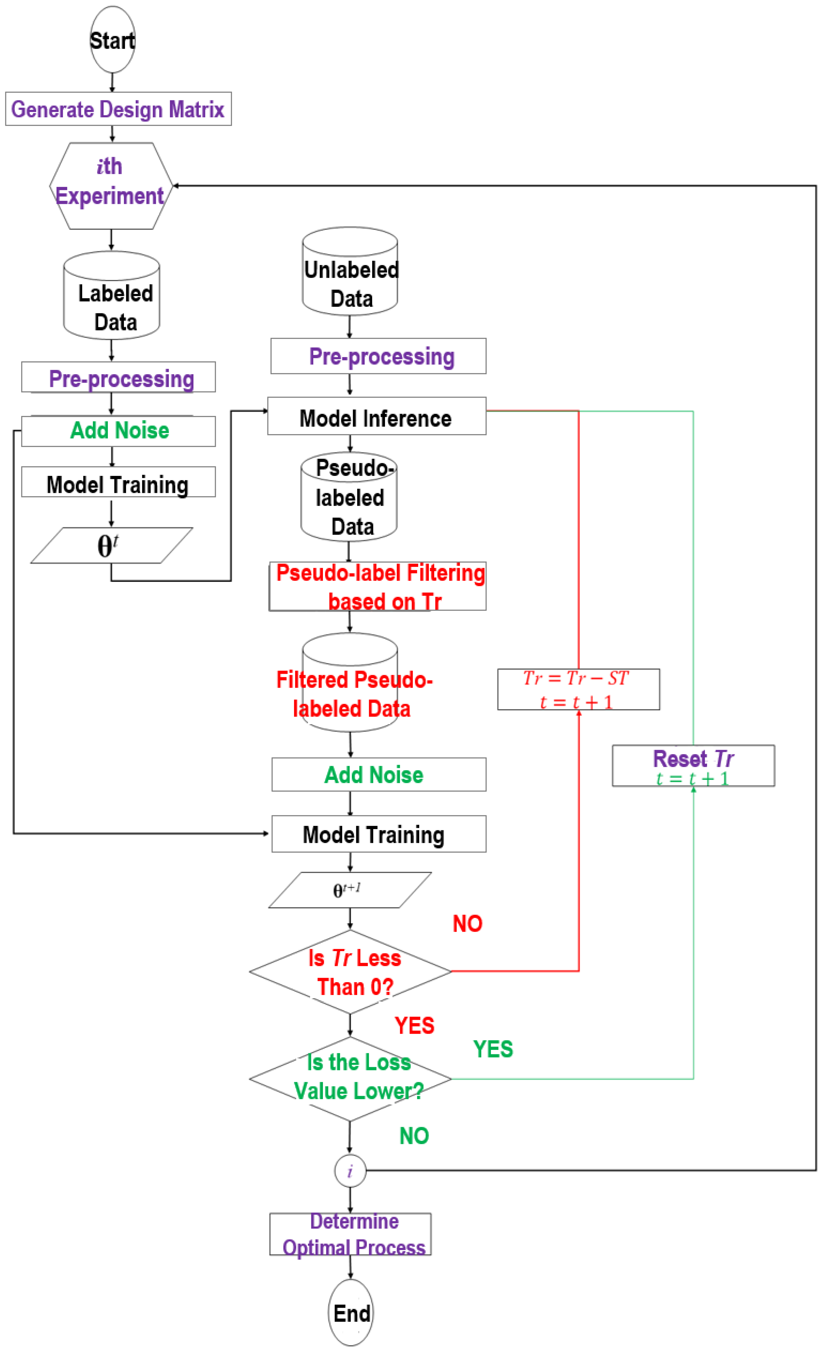
This study introduces a hybrid self-training algorithm that integrates pseudo-labeling [30], noisy student [31], curriculum learning [32], and the Taguchi method. The integration process is depicted in Figure 2. In the figure, the pseudo-labeling method is represented in black text. It utilizes a small amount of labeled data to train a CNN classifier, yielding an initial model. This model is then used to predict a large volume of unlabeled data, generating pseudo-labels to expand the dataset. The classifier is subsequently trained on both labeled and pseudo-labeled data.
The noisy student method, highlighted in green in Figure 2, builds upon pseudo-labeling. Noisy labeled data are used to train the initial model, after which noise is added to both the input labeled data and pseudo-labeled data during model training. This approach aims to enhance the model’s generalization capability. Moreover, the noisy student involves repetitive training of the CNN classifier until there is no further reduction in the loss function.
Curriculum learning, marked in red text and lines in Figure 2, also extends from the pseudo-labeling foundation. It refrains from adding noise and introduces a threshold for class probability (Tr). After obtaining the initial model, it is used for inferring unlabeled data. The predicted results are then filtered, and the model is trained with labeled data and the filtered pseudo-labeled data. Throughout the training, the Tr threshold is gradually reduced, incorporating more challenging data until all data is included in the training.
In the integration method proposed in this research, besides the concepts of pseudo-labeling, noisy student, and curriculum learning, additional elements, represented in purple text in Figure 2, are also included. The first element concerns the pre-processing of images to facilitate more suitable data for analysis. The second involves the incorporation of the Taguchi method, enabling the model to self-tune hyperparameters and autonomously select optimal processes. The overall process of the proposed hybrid self-training method is described as follows:
The hybrid self-training method integrates pseudo-labeling, noisy student, and curriculum learning methods. It starts by preparing labeled and unlabeled datasets. As shown in Equation (1), in the labeled dataset, xi represents input features and yi represents the corresponding class, indicating that each piece of data in the n entries has a corresponding class. As expressed in Equation (2), the m entries in the unlabeled dataset only have input features x̃i.
{(x1, y1), (x2, y2), …, (xi, yi), …, (xn, yn)}
{x̃1, x̃2, …, x̃i, …, x̃m}
As illustrated in Figure 2, the labeled data undergo image pre-processing and noise addition. The training of the CNN classifier then commences using the loss function L in Equation (3), leading to a model with parameters at t-th epoch θt.
Here, f(.) represents the CNN classifier, and CE(.) represents the cross-entropy function. The CNN classifier trained above is then applied to predict the unlabeled data after image pre-processing. The pseudo-labels corresponding to the unlabeled data are extracted through Equation (4)
where the class with the highest predicted class probability is chosen as its corresponding pseudo-label. In this equation, ỹi denotes the pseudo-label predicted by the model for the i-th unlabeled data entry. Subsequently, pseudo-labeled data with predicted class probabilities higher than the Tr are filtered. Noise is added to these filtered pseudo-labeled data. The CNN classifier is then trained with the noise-added labeled data and pseudo-labeled data using the loss function in Equation (5), resulting in a model with parameters θt+1.
In Equation (5), α(t) denotes the balance coefficient, which is used to balance the weights of the cross-entropy between labeled data and pseudo-labeled data. If the coefficient is set too high, the filtered pseudo-labeled data might interfere with the training. If set too low, they might not participate in the training at all. Lee suggested gradually increasing the balance coefficient as shown in Equation (6) to avoid obtaining suboptimal local solutions [30].
Here, αf, T1 and T2 are set to 3, 50, and 300, respectively. This means that α(t) is set to 0 for the first 50 iterations, and only labeled data is used for training. Between the 50th and 300th iterations, α(t) increases linearly, gradually enhancing the significance of the filtered pseudo-labeled data. After 300 iterations, α(t) is fixed at 3.
The process of inferring unlabeled data, filtering pseudo-labeled data, and training with both labeled and filtered pseudo-labeled data is iteratively executed. It starts with the initial value of Tr, reducing by 20% stepwise towards the threshold value (ST) until Tr is less than 0. This approach enables the CNN to initially learn from easily classified pseudo-labeled data and progressively introduce more complex pseudo-labeled data with lower predictive class probabilities into the training. As a result, CNN’s predictive capabilities gradually mature. The overall loss value is reviewed at the end; if it is lower, Tr is reset, and the training process continues; otherwise, the training concludes.
Details of each sub-function in Figure 2 are described as follows:

Figure 2.
Overview of the proposed hybrid self-training algorithm flowchart.
Figure 2.
Overview of the proposed hybrid self-training algorithm flowchart.
3.2.1. Sub-Function for “Generate Design Matrix”
Based on the number of factors and level numbers designed in the study, a design matrix can be obtained. In this matrix, each column represents a modeling strategy, and each row represents various experimental settings.
Evaluating CNN performance with various modeling strategies: Given the training data and the combination of training modeling strategies to enhance the predictive performance of the training classifier, the classifier will strive to optimize its hyperparameters using random search methods to obtain the best metrics for the training dataset. By repeating the above experiment for different modeling strategy combinations in random order, the experimental data of the design matrix can be completely collected.
3.2.2. Sub-Function for “Pre-Processing”
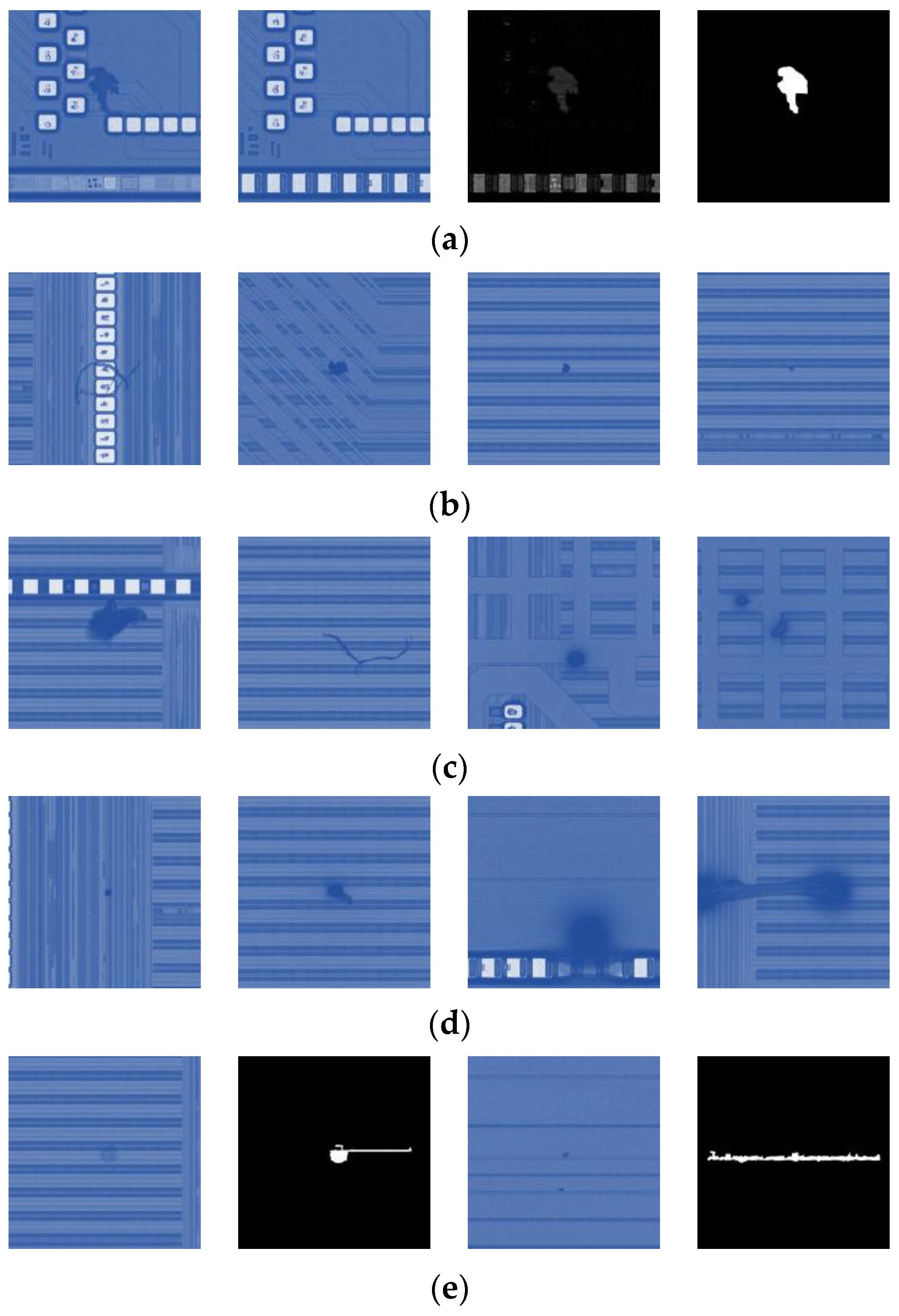
This study conducts image pre-processing on pictures captured by existing AOI machines, with the original image size being 720 × 720 × 3. The pre-processing targets both the raw images and corresponding defect masks, with the process illustrated in Figure 3. Occasionally, defect masks exhibit excessive lines or extensive noise due to alignment issues. To refine these masks, the algorithm evaluates the mask’s area and employs the Hough transform to detect lines. For defects not exceeding 10,000 pixels or those beyond 10,000 pixels but without lines, the brightness of the original image is directly adjusted. The pixels within the mask retain their grayscale values while those outside brighten, thereby diminishing background texture features and preventing classification domination by the background texture.
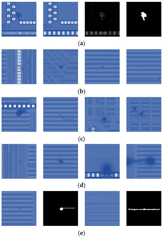
Figure 3.
The die images analyzed in this study showing (a) provided image pairs, (b) significant background variations, (c) uncentered defects, (d) large variations in defect sizes, and (e) mismatch between defect masks and defects.
If the defect area surpasses 10,000 pixels and contains lines, the line segment detector (LSD) is additionally applied to the defect mask for more precise line identification. If LSD fails to detect lines, the brightness of the original image is directly adjusted, both inside and outside the defect mask. When lines are identified, they are filtered according to length until no segments exceed 100 pixels. Following this, connected component labeling (CCL) identifies binary large objects (blobs), noting each blob’s number, area, centroid, and coordinate set while eliminating smaller blobs. If a blob’s coordinate set exists at the image’s central point, only that blob is retained; otherwise, the blob closest to the center is kept. The refined defect mask is then used to adjust the brightness of the original image.
Ultimately, utilizing the mask’s centroid coordinates, the original image is cropped to 150 × 150 × 3, and this segment is then outputted.
3.2.3. Sub-Function for “Add Noise”
By utilizing images infused with noise, the classifier learns to manage uncertainty and variability, enhancing its general predictive capability. Techniques including rotation, flipping, and brightness adjustment are incorporated in this study. Rotation slightly turns the original image to create different angles; flipping generates horizontally or vertically symmetrical images; brightness adjustment alters the pixel values to change the image’s brightness. It is essential in the noise addition subfunction to avoid introducing excessive and unrealistic noise, such as random masking or cropping.
3.2.4. Sub-Function for “Model Training”
Regarding the choice of CNN classifiers, this study employs the more representative VGGNet, ResNet, and DenseNet as encoders for feature extraction. VGGNet is a plain model. It operates by allowing the input image to pass through stacked convolutional layers to obtain a series of feature maps. Each convolution operation uses the same kernel size, and the number of kernels increases progressively to extract increasingly complex image features. After each convolution layer in VGGNet, there is a ReLU activation function. The feature maps then pass through a pooling layer to reduce the image size, enhancing the rotation, translation, and deformation invariance of the features. Finally, the feature maps are flattened into a one-dimensional vector for classification by the fully connected layer.
ResNet first passes the input image through a convolution layer and a pooling layer to obtain a smaller feature map. The feature map then undergoes processing by multiple residual blocks. Each residual block comprises several convolution layers and shortcut connections. Shortcut connections involve adding a channel between convolution layers, allowing information to bypass some layers and be directly added to the output elements of the convolution layer, mitigating model degradation and vanishing gradient issues during training. Convolution blocks for downsampling are inserted between residual blocks to reduce image size. After the feature enhancement through multiple residual blocks and convolution blocks, a global average pooling (GAP) layer flattens the feature map into a one-dimensional vector, leading to classification by the fully connected layer. Every convolution layer in ResNet is accompanied by a BN layer and a ReLU activation function.
DenseNet initially processes the input image via a convolution layer followed by a pooling layer, resulting in a reduced-size feature map. Subsequently, this feature map undergoes processing through multiple dense blocks. Each block encompasses numerous skip connections originating from the outputs of prior convolution layers, facilitating the aggregation of feature maps along the channel dimension. Transition layers for downsampling are placed between dense blocks to reduce the image size. After the feature reinforcement from multiple dense blocks and transition layers, a GAP layer flattens the feature map into a one-dimensional vector for classification by the fully connected layer. Each convolution layer in DenseNet is followed by a BN layer and a ReLU activation function.
3.2.5. Sub-Function for “Model Inference”
Model inference involves using a trained model to predict unseen and unlabeled images. The process includes inputting an image, running it through the trained CNN classifier, and outputting predictions with associated class probabilities, indicating the likelihood of each possible class and helping to assess the model’s confidence in its predictions.
3.2.6. Sub-Function for “Pseudo-Label Filtering”
After model inference, class probabilities can be used with underling Tr to select high-confidence unlabeled images. These images are then assigned pseudo-labels, enhancing the dataset for further training or validation and ultimately improving the model’s performance and accuracy.
3.2.7. Sub-Function for “Determine Optimal Process”
During the training mode process, several modeling strategies can be adopted to enhance the model’s predictive capability. However, no combination of modeling strategies has been proven to be the best, as everything depends on the distribution of the dataset. Consequently, sensitivity analysis is required when users are training the model. By considering the modeling strategy as a factor, where each modeling strategy is based on different level numbers, and taking the classification accuracy of the training data as the dependent variable, the procedure of the Taguchi experiment can be established to systematically carry out modeling strategy selection. Plotting the main effect plot can assist in selecting the optimal combination of modeling strategies. Whether to incorporate a particular training strategy into model training is determined by the performance of each training strategy at each level.
The overall pseudo code of Figure 2 is described in the Appendix A, which provides a Python-structured representation of the proposed hybrid self-training algorithm, facilitating a better understanding of its implementation.
3.3. Model Evaluation Metrics
For multi-class classification tasks, a multi-class confusion matrix, as illustrated in Table 1, is commonly used. This matrix serves to summarize actual and predicted results, facilitating the calculation of various metrics. The confusion matrix consists of K rows and columns, where K represents the total number of classes. In this matrix, rows account for the true values of each class, while columns consider the predicted values for each class. Consequently, the diagonal elements C1,1, C2,2, …, CK,K represent the number of samples correctly predicted, while the off-diagonal elements indicate the number of samples where the model misclassified the true class as another class.

Table 1.
Schematic diagram of the confusion matrix for multi-class classification tasks.
By analyzing the aforementioned multi-class confusion matrix, various metrics can be calculated to evaluate the overall performance of the model, including accuracy, precision, macro precision, recall, macro recall, and macro F1-score expressed, respectively, in Equations (7)–(12).
Accuracy = (C1,1 + C2,2 + … + CK,K)/(C1,1 + C1,2 + … + CK,K)
Precisionk = Ck,k/(Ck,1 + Ck,2 + … + Ck,k), k = 1, 2, …, K
Macro Precision = (Precision1 + Precision2 + … + PrecisionK)/K
Recallk = Ck,k/(C1,k + C2,k + … + Ck,k), k = 1, 2, …, K
Macro Recall = (Recall1 + Recall2 + … + RecallK)/K
Macro F1-score = 2(Macro Precision × Macro Recall)/(Macro Precision + Macro Recall)
4. Experimental Analysis and Results Presentation
This chapter is divided into three sections. The first section provides an introduction to the images of each class. The second section explains the reasons for choosing various levels of each factor and the use of the Taguchi method for sensitivity experimentation and analyzes the optimal combination of hyperparameters. The final section compares the die defect classification results between the tuned self-training algorithms and supervised learning, presenting their comparative outcomes. The hardware setup includes an Intel® Xeon® Silver 4214 CPU running at 2.20 GHz, equipped with 96.0 GB of DDRAM, and supported by an NVIDIA V100S-32Q GPU. The hardware equipment is sourced from DELL in Penang, Malaysia. On the software side, the research relies on a Python environment configured with essential packages such as torch, PIL, cv2, sklearn, and dexpy.factorial. These specifications collectively provide the necessary computational power and software tools required to successfully carry out the experiments in the study.
4.1. Description of Image Dataset
The die dataset used in this study was provided by a semiconductor manufacturer in Taiwan. This manufacturer utilizes an existing AOI system to capture images of dies on the production line. Due to a confidentiality agreement, all die images displayed in the study have undergone color transformation, flipping, and cropping. The image set encompasses the following characteristics that make the dataset challenging for classification:
- Providing image pairs. For each defective image, the manufacturer provides four paired images, as shown in Figure 3a. These include the original image, the corresponding golden template, the residual map, and the binarized defect mask. This study only utilizes the original images and defect masks for analysis.
- Significant background variations. As depicted in Figure 3b, the customization of die patterns for different clients results in a significant variety in the structure and coloration of the dies. Additionally, the AOI system captures only the defect areas, leading to a dramatic increase in the background variation of the images analyzed.
- Defects are not centered. Despite the AOI system’s attempt to center the defects during image capture, there are instances where the defects are not centered, as shown in Figure 3c.
- Large variations in defect sizes. Even within the same defect class, there is a considerable size variation. Small defects may be only 10 pixels in size, while larger ones can span half the width of an image, as illustrated in Figure 3d.
- Mismatch between defect masks and defects. The defect masks do not always align perfectly with the actual defect contours in the original images. Slight deviations in the AOI system’s template matching can lead to additional defect pixels appearing within the defect masks, as shown in Figure 3e.
In this study, we performed experiments using two sets of die defect images captured by the AOI machine: a small-scale set and a large-scale set. The small-scale set comprised 3924 die defect images, classified into six defect classes. Figure 4a presents these six defect types after image preprocessing. In contrast, the large-scale set consisted of 13,909 die defect images, segmented into fourteen defect classes. Figure 4b illustrates the additional eight defect types after image preprocessing. The large-scale set includes the initial six types shown in Figure 4a and introduces eight additional defect types in Figure 4b. We allocated 80% of these images to the training dataset and the remaining 20% to the testing dataset.
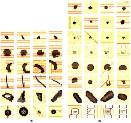
Figure 4.
Preprocessed images of defective dies for each class. (a) The initial six defect types in the small-scale set; (b) eight additional defect types in the large-scale set.
4.2. Factor Levels and Sensitivity Analysis
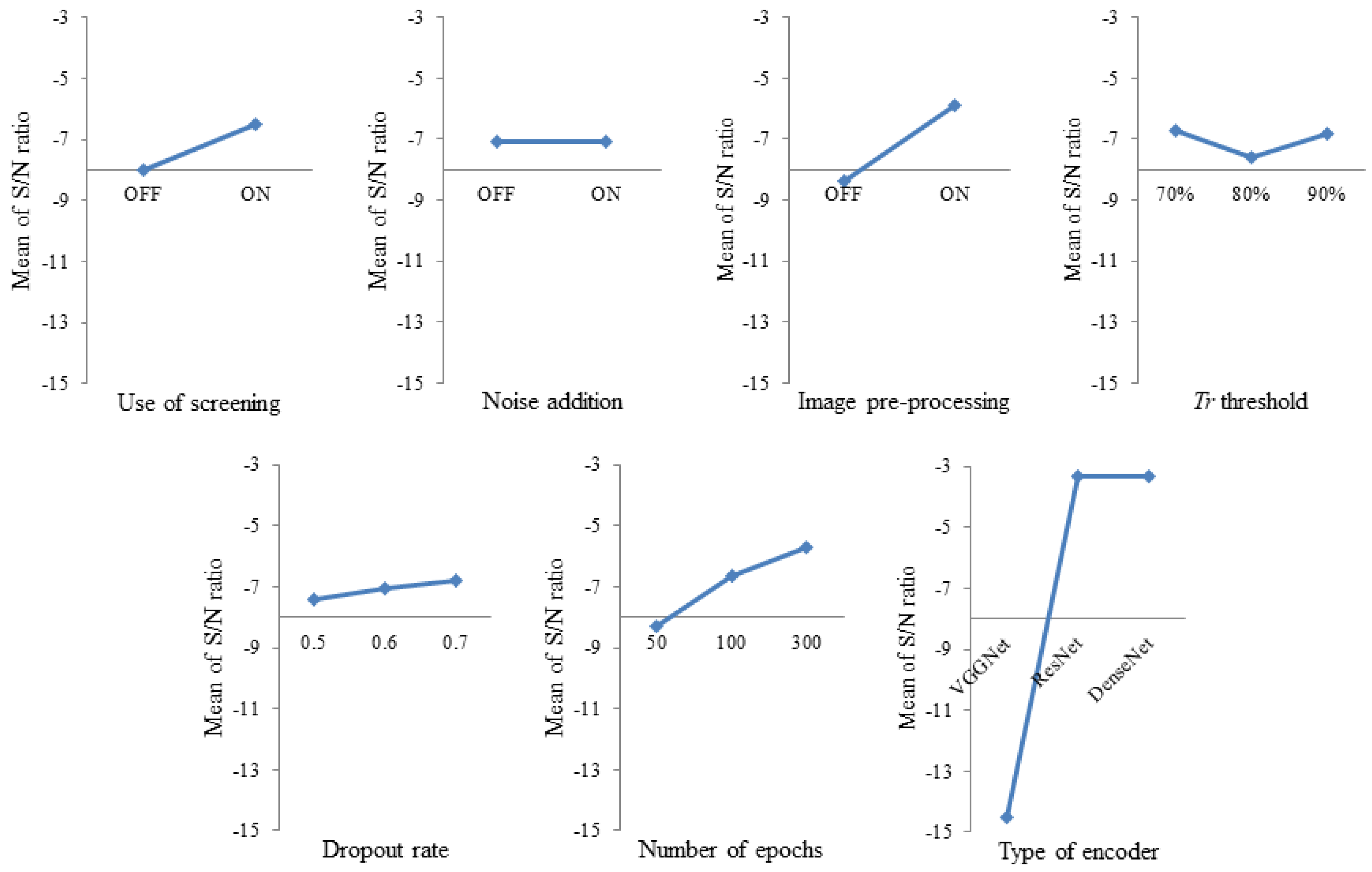
In this study, the Taguchi method was used to optimize the hyper-parameter combinations of our hybrid self-training algorithm. It plays a pivotal role in the model training process and subsequent inference performance. We selected eight factors with different levels and designed a set of experiments that systematically varied these factors using orthogonal arrays, reducing the number of required experiments while ensuring comprehensive data collection. We evaluated the model’s performance for each experimental setup using metrics. The main effects plot for the signal-to-noise (S/N) ratio helped us visualize the impact of each factor on performance, guiding us to adjust them for optimal results. By incorporating the Taguchi method, we ensured a systematic and efficient approach to hyper-parameter combinations with a minimal number of experiments, leading to a more robust semi-supervised die defect classification model.
In this study, seven factors are set, with three of them having two levels and the remaining four having three levels. Each factor and its corresponding levels are presented in Table 2, with elaboration and utilization described as follows:

Table 2.
Settings of factors and levels using Taguchi method.
- Use of screening: This factor pertains to the activation status of screening. The levels for this factor are defined according to the proposed research methodologies. Selecting “ON” indicates the employment of the curriculum learning technique, which involves selecting unlabeled data with a classification prediction probability above a specified threshold and progressively reducing this threshold to escalate the learning challenge. Selecting “OFF” denotes that the screening process is not implemented.
- Noise addition: This factor considers whether noise is added or not, and the level options are based on the proposed research methods. Selecting “ON” denotes the implementation of the noisy student technique, applying image augmentation, including rotation, horizontal flipping, and brightness adjustment, before the model training process. Choosing “OFF” indicates no use of image augmentation.
- Image pre-processing: This factor is intended to determine whether to enable image pre-processing. The level options are established based on the proposed research methods. Selecting “ON” signifies that a series of pre-processing procedures, including line segment removal from masks, brightness adjustment inside and outside the masks, and image cropping, are performed before feeding images into the model. Choosing “OFF” indicates that the model is fed with raw images without any pre-processing.
- Tr threshold: This is a screening threshold used to select unlabeled data with a classification prediction probability exceeding Tr to generate pseudo-labels. The level choices for this factor, set at 70%, 80%, and 90%, are based on [33]. If the value is set too low, it would easily assign pseudo-labels to any unlabeled data, reducing the reliability of these labels and affecting the quality of model training.
- Dropout rate: This is a regularization technique used to prevent model overfitting. The level choices for this factor, namely 0.5, 0.6, and 0.7, are based on [34]. The dropout mechanism randomly omits a portion of neurons during each training batch, forcing the model not to rely on specific neurons for predictions and thereby enhancing the model’s generalization capability.
- Number of epochs: This refers to the number of times the model sees the entire dataset of images during the training process. The level choices, set at 50, 100, and 300, are based on the default parameters of the balancing coefficient shown in Equation (6). The balancing coefficient allows the model to linearly increase the proportion of unlabeled images considered during the calculation of the loss function as the steps increase.
- Type of encoder: Encoders are used to extract crucial features from images. Different encoders have distinct structures and functions, and their adaptability varies for specific tasks. The level choices for this factor, namely, VGGNet, ResNet, and DenseNet, are based on [25]. Choosing the appropriate encoder helps in determining the best feature extraction network structure for specific tasks to achieve better classification accuracy.
The experimental results were analyzed using the Taguchi method for larger-the-better criteria, and the main effects plot for the S/N ratio is depicted in Figure 5. The conclusions drawn from the experiment reveal that the performance of implementing filtering is superior to not implementing it, indicating that confidence screening of unlabeled data yields better modeling results. Performance without adding noise is more optimal, suggesting the effectiveness of abstaining from data augmentation during the training process. Models that undergo pre-processing exhibit superior performance, emphasizing the benefits of pre-processing the data. When the Tr threshold is set at 70%, the performance surpasses settings at 80% and 90%, illustrating that a lower initial Tr threshold allows the CNN model to commence learning with moderately challenging samples, effectively enhancing performance. A dropout rate set at 0.7 outperforms 0.6 and 0.5, indicating that a moderate dropout rate aids in preventing overfitting and enhances the model’s generalization capability. A step setting of 300 is more effective than 50 and 100, demonstrating that a larger number of steps enables better learning of data features, offering more opportunities for iterative learning and accuracy enhancement. When DenseNet is selected as the encoder, it outperforms ResNet and VGGNet, proving that DenseNet’s feature reuse mechanism is more efficient than ResNet’s residual module and VGGNet’s multi-layer convolution.
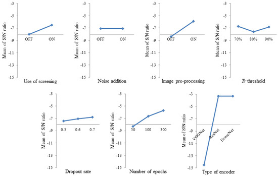
Figure 5.
Main effects plot for S/N ratio from the Taguchi experiment (larger-the-better).
4.3. Comparison of Die Classification Results among Various Algorithms
Based on [25], our study conducted experiments with 50%, 25%, and 10% proportions of labeled data to evaluate the classification performance of the model under various scales of labeled data volume. This also demonstrated the adaptive ability of the methodology proposed in this study.
Initially, experiments were carried out with 50% of the data being labeled. The optimal combination of hyperparameters for each factor was identified through the Taguchi method. We decided to adopt curriculum learning, turn off the noisy student, set the Tr threshold to 70%, establish a dropout rate of 0.7, set the steps to 300, and select DenseNet as the encoder. This implies that curriculum learning has adaptively emerged as the recommended approach for semi-supervised modeling of the training dataset in our study. To achieve the objective of method comparison, we fixed the optimal modeling strategy mentioned above and used the test image set for performance comparison among various methods. These methods include supervised DenseNet, pseudo-labeling, noisy student, curriculum learning, and a hybrid approach.
The comparison results for the small-scale set, with a labeled data proportion of 50% as shown in Table 3, reveal that the curriculum learning recommended by our study outperformed the other four algorithms in terms of classification accuracy, precision, and recall rates. Its accuracy, macro precision, macro recall, and macro F1-score were approximately 25% higher than those of supervised DenseNet, around 8% higher than pseudo-labeling, about 7% better than the noisy student, and approximately 4% better than the most complex hybrid method.

Table 3.
Summary of classification results of various algorithms on a small-scale dataset at different proportions of labeled data.
In addition to the performance comparison among various methods with 50% labeled data, our study also explored scenarios with 25% and 10% labeled data. The comparison results for these proportions of labeled data are presented in Table 3. The outcomes indicate that the situation with 25% labeled data mirrors that of 50%, where curriculum learning is adaptively recommended. This method also yielded the best results in terms of accuracy, macro precision, macro recall, and macro F1-score. Interestingly, when the proportion of labeled data was reduced to 10%, the hybrid method was adaptively recommended. It yielded accuracy, macro precision, macro recall, and macro F1-score that were slightly higher or comparable to those of curriculum learning. This suggests that the hybrid method can be particularly effective in scenarios where the proportion of labeled data is extremely low.
Furthermore, the experiment also revealed that the classification performance with 50% labeled data exceeds that with 10% and 25%. This implies that a lower proportion of labeled data constrains the learning capacity of the model. When the model is trained using only a small amount of labeled data, it struggles to cope with datasets where high similarity exists among samples.
In another experiment with a large-scale set, we compared the performance of various algorithms, including DenseNet, pseudo-labeling, noisy student, curriculum learning, and the hybrid method, at different proportions of labeled data (50%, 25%, and 10%). Our analysis revealed distinct performance metrics in terms of accuracy, macro precision, macro recall, and macro F1-score, as summarized in Table 4.

Table 4.
Summary of classification results of various algorithms on a large-scale dataset at different proportions of labeled data.
At a labeled data proportion of 50%, the hybrid method demonstrated the highest classification accuracy at 88.75%, surpassing the other algorithms. It also led in macro precision (87.14%), macro recall (86.14%), and macro F1-score (86.46%) among the competitors, indicating its superior efficiency in handling the large-scale set. Curriculum learning followed closely in accuracy (87.46%) and exhibited competitive precision, recall, and F1-score. In the scenario with 25% labeled data, the hybrid method again outperformed the others, achieving an accuracy of 86.31%, with the highest macro precision (85.41%), macro recall (83.29%), and macro F1-score (84.24%). Curriculum learning showed strong performance, especially in accuracy (85.41%) and precision (84.14%), highlighting its viability as a competitive approach. At the 10% labeled data level, the hybrid method stood out with the highest accuracy (83.61%), macro precision (81.21%), macro recall (80.50%), and macro F1-score (80.85%), solidifying its effectiveness in scenarios with minimal labeled data. Pseudo-labeling emerged as the second-best-performing algorithm in terms of accuracy (81.24%), overtaking curriculum learning.
This experiment illustrates the adaptability and efficiency of the proposed hybrid method, rendering it particularly effective for large-scale sets with varying proportions of labeled data. The findings suggest a trend in which the proportion of labeled data inversely affects the learning capability of the model, with higher proportions generally resulting in better classification performance.
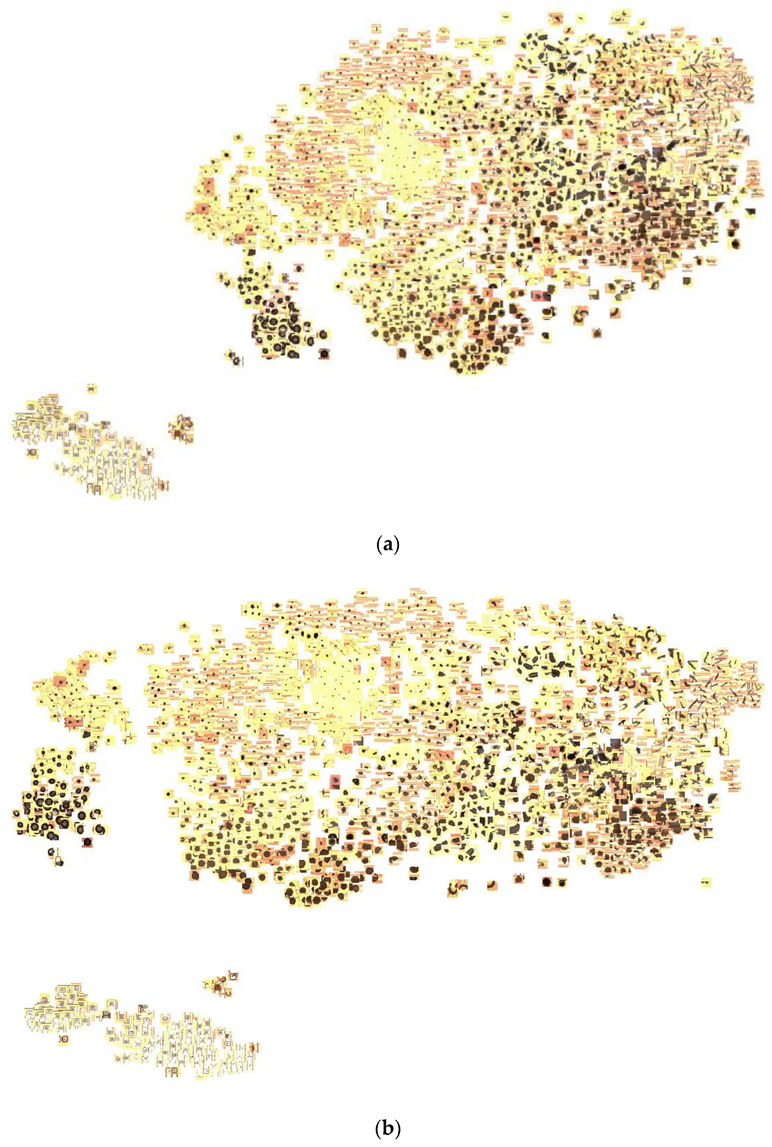
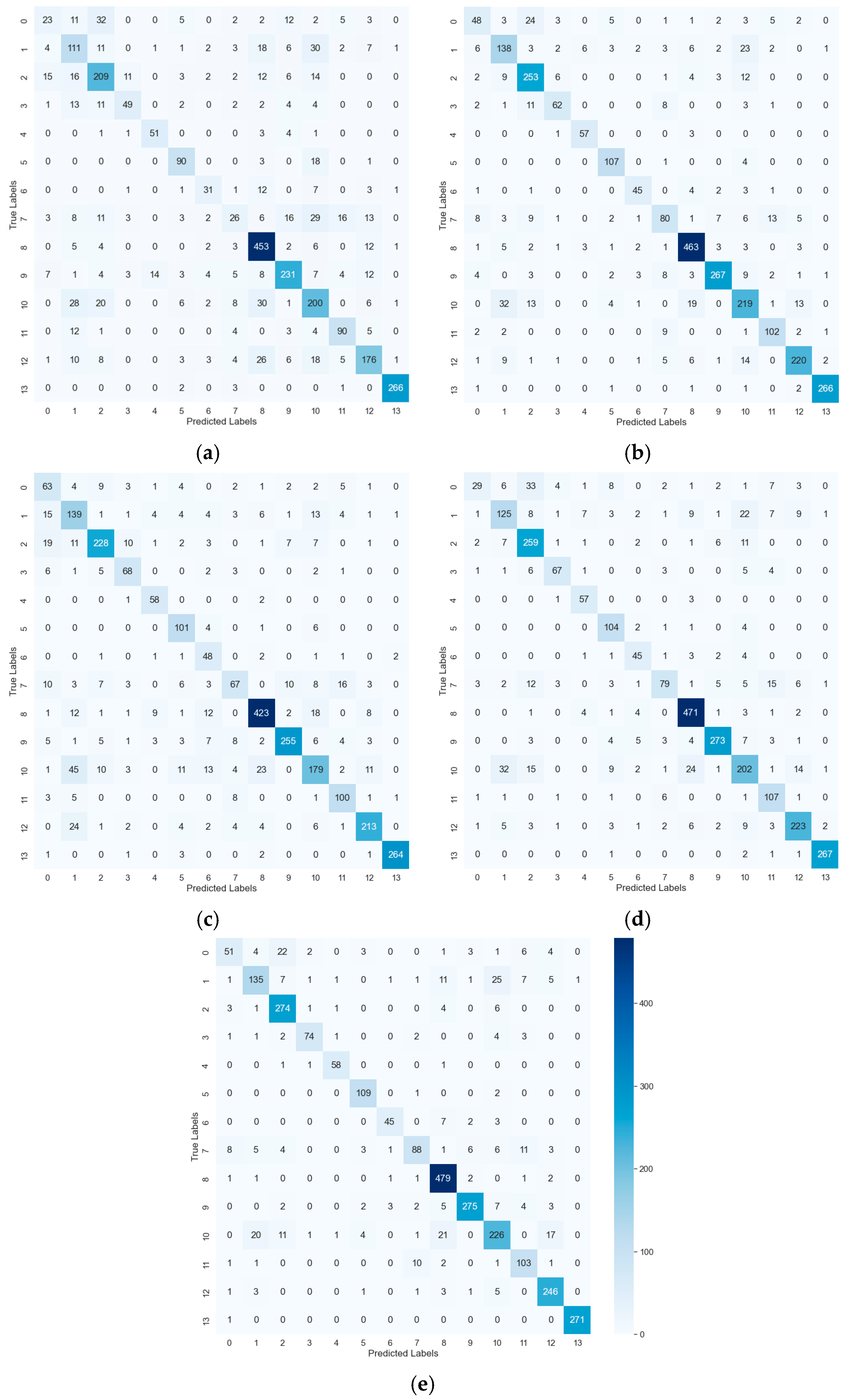
Moreover, in this study, for the case where the labeled data ratio is 10%, the features extracted from all test data by five methods are mapped to a low-dimensional space using t-distributed stochastic neighbor embedding (t-SNE). Observing the phenomenon of similar images clustering together in the t-SNE plot indicates that these images are similar in the high-dimensional feature space and can be mapped to adjacent positions in the low-dimensional t-SNE space. As shown in Figure 6a–e and Figure 7a–e, this study provides the t-SNE plots and confusion matrices after classification prediction for each method, respectively. As shown in Figure 6d,e and Figure 7d,e, the clustering in the t-SNE plot of curriculum learning and the hybrid method are distinct, with clear boundaries between classes. It can be observed that methods with higher classification accuracy have similar images that are relatively closer together in the t-SNE plot, while dissimilar images are located in different areas. However, dissimilar images with similar appearances are distributed in adjacent areas, further demonstrating the excellent feature extraction capabilities of these algorithms. In contrast, the images in the t-SNE plot of pseudo-labeling, as shown in Figure 6b and Figure 7b, are more evenly distributed. The larger gaps between clusters indicate its advantage in handling noisy data and distinguishing classes effectively. As shown in Figure 6c and Figure 7c, the noisy student t-SNE plot shows good clustering with some confusion. It is worth noting that the clustering in the t-SNE plot of supervised DenseNet shown in Figure 6a and Figure 7a is relatively tight. The central region is overly dense, which may lead to more inter-class confusion. Because the positions of dissimilar images are not well separated, its classification ability is naturally inferior to that of other semi-supervised methods.

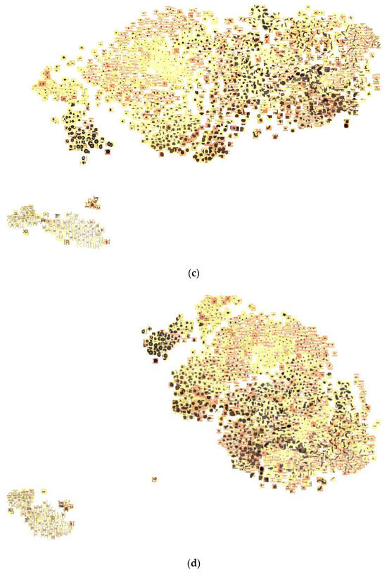
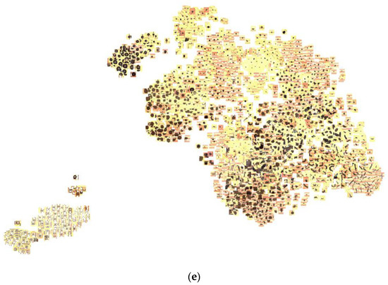
Figure 6.
t-SNE plots of various algorithms on the large-scale set with 10% labeled data. (a) Supervised DenseNet, (b) pseudo-labeling, (c) noisy student, (d) curriculum learning, (e) hybrid method.
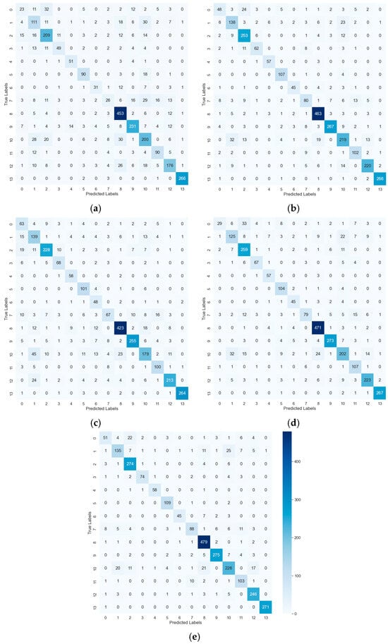
Figure 7.
Confusion matrices of various algorithms on the large-scale set with 10% labeled data. (a) Supervised DenseNet, (b) pseudo-labeling, (c) noisy student, (d) curriculum learning, (e) hybrid method.
5. Conclusions and Suggestions
This study focused on images of die defects, employing the Hough transform and line segment detector to identify and highlight defect lines, modify defect shapes, and concurrently adjust brightness within and outside the mask to enhance the visibility of features in the die defect images. To optimize the modeling strategy, Taguchi’s method was applied in a mixed experiment involving three 2-level and four 3-level factors. The results demonstrated that with filtering enabled, image preprocessing activated, a threshold of 70%, a dropout rate of 0.7, 300 steps, and the DenseNet encoder selected, the model exhibited superior performance on a small-scale set with only 50% labeled data, achieving a classification accuracy of 92.81%. Particularly, compared to supervised DenseNet, the accuracy was surpassed by more than 20%. Even when the proportion of the labeled dataset was reduced to 25% and 10%, the classification accuracy of the proposed method remained robust. For another large-scale set, the proposed hybrid method dominated across all metrics, suggesting it as a potent solution for achieving high classification accuracy.
In the highly competitive landscape of IC manufacturing, where precision and quality control are paramount, the semi-supervised classifier introduced in this study proves to be a crucial advancement. It effectively categorizes defects in die images, marking a significant step forward in automating and refining the inspection process. By leveraging this algorithm, IC companies can substantially reduce the time and costs associated with manual feature engineering and data labeling. This not only boosts the efficiency of die inspections but also significantly improves their accuracy, ensuring higher quality control standards are met with less resource expenditure.
Finally, we outline the key limitations and challenges encountered during our research. The dataset used in this study is primarily sourced from a single semiconductor manufacturer in Taiwan. This limitation may restrict the applicability of our model to other manufacturing environments. Future work should involve validating the model on more diverse datasets to ensure its broader applicability. Additionally, with evolving die patterns and manufacturing processes, the model needs continuous learning and updates to maintain classification efficacy. Establishing effective mechanisms for continuous learning and image updating is essential.
Author Contributions
Conceptualization, P.-H.W.; methodology, S.-H.C., Y.-T.C. and Y.-W.L.; software, Y.-T.C. and Y.-W.L.; validation, S.-H.C.; formal analysis, S.-Z.L., Y.-T.C. and Y.-W.L.; data curation, P.-H.W. and S.-H.C.; writing—original draft preparation, S.-Z.L. and S.-H.C.; writing—review and editing, S.-Z.L. and S.-H.C.; project administration, P.-H.W. and S.-H.C.; funding acquisition, P.-H.W. and S.-H.C. All authors have read and agreed to the published version of the manuscript.
Funding
This research was funded by National Science and Technology Council (NSTC), grant number 110-2221-E-131-026-MY3 and The APC was funded by Ming Chi University of Technology.
Data Availability Statement
The data used in this study were provided by the Product Testing Service Office, Nanya Technology Corporation, New Taipei City.
Conflicts of Interest
The authors declare that this study received funding from [Nanya Technology Corporation, Ming Chi University of Technology]. P.-H.W. and S.-H.C. were responsible for acquiring the funding. The funder had the following involvement with the study: P.-H.W. contributed to conceptualization, data curation, and project administration; S.-H.C. was involved in methodology development, validation, data curation, writing—original draft preparation, writing—review and editing, and project administration. Other authors declare no conflicts of interest.
Appendix A
| # Pseudo Code of Hybrid Self-training algorithm # Given datasets labeled_data unlabeled_data # Set hyper-parameters ST = 0.2 alpha_f = 3 T1 = 50 T2 = 300 # Set factors and levels for Taguchi method factors = [‘use_of_screening’, ‘noise_addition’, ‘image_preprocessing’, ‘Tr_threshold’, ‘dropout_rate’, ‘number_of_epochs’, ‘type_of_encoder’] levels = { ‘use_of_screening’: [True, False], ‘noise_addition’: [True, False], ‘image_preprocessing’: [True, False], ‘Tr_threshold’: [0.7, 0.8, 0.9], ‘dropout_rate’: [0.5, 0.6, 0.7], ‘number_of_epochs’: [50, 100, 300], ‘type_of_encoder’: [‘VGGNet’, ‘ResNet’, ‘DenseNet’] } # Perform Taguchi experiment to determine optimal settings design_matrix = generate_design_matrix(factors, levels) metric_collector = [] for exp in design_matrix: # Train an initial CNN classifier if exp.image_preprocessing: labeled_data = preprocessing(labeled_data) if exp.noise_addition: labeled_data = add_noise(labeled_data) theta, loss, metrics = model_training(exp.type_of_encoder, theta, labeled_data, exp.dropout_rate, exp.number_of_epochs, alpha_f, T1, T2) # Pseudo-labeling unlabeled data if exp.image_preprocessing: unlabeled_data = preprocessing(unlabeled_data) pseudo_labeled_data = model_inference(theta, unlabeled_data) # Iterative training with pseudo-labeled data if exp.use_of_screening: Tr_threshold = exp.Tr_threshold while True: filtered_pseudo_labeled_data = pseudo_labeled_filtering(pseudo_labeled_data, Tr_threshold) if exp.noise_addition: filtered_pseudo_labeled_data = add_noise(filtered_pseudo_labeled_data) theta_new, loss_new, metrics = model_training(exp.type_of_encoder, theta, [labeled_data, filtered_pseudo_labeled_data], exp.dropout_rate, exp.number_of_epochs, alpha_f, T1, T2) Tr_threshold = Tr_threshold - ST # Check if Tr_threshold is less than 0 if Tr_threshold < 0: break # Check if the new loss value is lower if new_loss < loss: theta = theta_new loss = loss_new metric_collector = metrics_collector.append(metrics) else: Tr_threshold = exp.Tr_threshold # Increment time t = t + 1 optimal_setting = determine_optimal_process(design_matrix, metric_collector) |
References
- Mital, D.P.; Teoh, E.K. Computer based wafer inspection system. In Proceedings of the IECON’91: 1991 International Conference on Industrial Electronics, Control and Instrumentation, Kobe, Japan, 28 October 1991—1 November 1991; pp. 2497–2503. [Google Scholar]
- Tobin, K.W., Jr.; Karnowski, T.P.; Lakhani, F. Integrated applications of inspection data in the semiconductor manufacturing environment. In Metrology-Based Control for Micro-Manufacturing; International Society for Optics and Photonics: Bellingham, WA, USA, 2001; Volume 4275, pp. 31–40. [Google Scholar]
- Chou, P.B.; Rao, A.R.; Sturzenbecker, M.C.; Wu, F.Y.; Brecher, V.H. Automatic defect classification for semiconductor manufacturing. Mach. Vis. Appl. 1997, 9, 201–214. [Google Scholar] [CrossRef]
- Zhang, J.M.; Lin, R.M.; Wang, M.J.J. The development of an automatic post-sawing inspection system using computer vision techniques. Comput. Ind. 1999, 40, 51–60. [Google Scholar] [CrossRef]
- Guan, S.U.; Xie, P.; Li, H. A golden-block-based self-refining scheme for repetitive patterned wafer inspections. Mach. Vis. Appl. 2003, 13, 314–321. [Google Scholar] [CrossRef][Green Version]
- Liu, H.; Zhou, W.; Kuang, Q.; Cao, L.; Gao, B. Defect detection of IC wafer based on two-dimension wavelet transform. Microelectron. J. 2010, 41, 171–177. [Google Scholar] [CrossRef]
- Li, H.; von Kleist-Retzow, F.T.; Haenssler, O.C.; Fatikow, S.; Zhang, X. Multi-target tracking for automated RF on-wafer probing based on template matching. In Proceedings of the 2019 International Conference on Manipulation, Automation and Robotics at Small Scales (MARSS), Helsinki, Finland, 1–5 July 2019; pp. 1–6. [Google Scholar]
- Su, C.T.; Yang, T.; Ke, C.M. A neural-network approach for semiconductor wafer post-sawing inspection. IEEE Trans. Semicond. Manuf. 2002, 15, 260–266. [Google Scholar]
- Chang, C.Y.; Chang, C.H.; Li, C.H.; Jeng, M. Learning vector quantization neural networks for LED wafer defect inspection. In Proceedings of the Second International Conference on Innovative Computing, Information and Control (ICICIC 2007), Kumamoto, Japan, 5–7 September 2007; p. 229. [Google Scholar]
- Timm, F.; Barth, E. Novelty detection for the inspection of light-emitting diodes. Expert Syst. Appl. 2012, 39, 3413–3422. [Google Scholar] [CrossRef]
- Jizat, J.A.M.; Majeed, A.P.A.; Nasir, A.F.A.; Taha, Z.; Yuen, E. Evaluation of the machine learning classifier in wafer defects classification. ICT Express 2021, 7, 535–539. [Google Scholar] [CrossRef]
- Cheon, S.; Lee, H.; Kim, C.O.; Lee, S.H. Convolutional neural network for wafer surface defect classification and the detection of unknown defect class. IEEE Trans. Semicond. Manuf. 2019, 32, 163–170. [Google Scholar] [CrossRef]
- Lin, H.; Li, B.; Wang, X.; Shu, Y.; Niu, S. Automated defect inspection of LED chip using deep convolutional neural network. J. Intell. Manuf. 2019, 30, 2525–2534. [Google Scholar] [CrossRef]
- Chen, X.; Chen, J.; Han, X.; Zhao, C.; Zhang, D.; Zhu, K.; Su, Y. A light-weighted CNN model for wafer structural defect detection. IEEE Access 2020, 8, 24006–24018. [Google Scholar] [CrossRef]
- Saqlain, M.; Jargalsaikhan, B.; Lee, J.Y. A voting ensemble classifier for wafer map defect patterns identification in semiconductor manufacturing. IEEE Trans. Semicond. Manuf. 2019, 32, 171–182. [Google Scholar] [CrossRef]
- Chen, S.H.; Kang, C.H.; Perng, D.B. Detecting and measuring defects in wafer die using GAN and YOLOv3. Appl. Sci. 2020, 10, 8725. [Google Scholar] [CrossRef]
- Yang, X.; Song, Z.; King, I.; Xu, Z. A Survey on Deep Semi-supervised Learning. arXiv 2021, arXiv:2103.00550. [Google Scholar] [CrossRef]
- Gordon, J.; Hernández-Lobato, J.M. Combining deep generative and discriminative models for Bayesian semi-supervised learning. Pattern Recognit. 2020, 100, 107156. [Google Scholar] [CrossRef]
- Zhang, S.; Ye, F.; Wang, B.; Habetler, T.G. Semi-supervised bearing fault diagnosis and classification using variational autoencoder-based deep generative models. IEEE Sens. J. 2020, 21, 6476–6486. [Google Scholar] [CrossRef]
- Chen, J.; Wang, Y.; Zhang, L.; Liu, M.; Plaza, A. DRFL-VAT: Deep representative feature learning with virtual adversarial training for semisupervised classification of hyperspectral image. IEEE Trans. Geosci. Remote Sens. 2022, 60, 5532914. [Google Scholar] [CrossRef]
- Noroozi, V.; Bahaadini, S.; Zheng, L.; Xie, S.; Philip, S.Y. Virtual adversarial training for semi-supervised verification tasks. In Proceedings of the 2019 27th European Signal Processing Conference (EUSIPCO), A Coruna, Spain, 2–6 September 2019; pp. 1–5. [Google Scholar]
- Liao, W.; Yang, D.; Wang, Y.; Ren, X. Fault diagnosis of power transformers using graph convolutional network. CSEE J. Power Energy Syst. 2020, 7, 241–249. [Google Scholar]
- Do, J.; Kim, M. Wafer map defect pattern classification with progressive pseudo-labeling balancing. In Proceedings of the Korean Society of Broadcast Engineers Conference, Online, 27–28 November 2020; pp. 248–251. [Google Scholar]
- Zhuo, X.; Rahfeldt, W.; Zhang, X.; Doros, T.; Son, S.W. DAP-SDD: Distribution-aware pseudo labeling for small defect detection. Comput. Sci. Math. Forum 2022, 3, 5. [Google Scholar] [CrossRef]
- Kahng, H.; Kim, S.B. Self-supervised representation learning for wafer bin map defect pattern classification. IEEE Trans. Semicond. Manuf. 2020, 34, 74–86. [Google Scholar] [CrossRef]
- Liu, T.; Ye, W. A semi-supervised learning method for surface defect classification of magnetic tiles. Mach. Vis. Appl. 2022, 33, 35. [Google Scholar] [CrossRef]
- Wang, C.; Jin, S.; Guan, Y.; Liu, W.; Qian, C.; Luo, P.; Ouyang, W. Pseudo-labeled auto-curriculum learning for semi-supervised keypoint localization. arXiv 2022, arXiv:2201.08613. [Google Scholar]
- Kim, Y.; Lee, J.S.; Lee, J.H. Automatic defect classification using semi-supervised learning with defect localization. IEEE Trans. Semicond. Manuf. 2023, 36, 476–485. [Google Scholar] [CrossRef]
- Qiao, Y.; Mei, Z.; Luo, Y.; Chen, Y. DeepSEM-Net: Enhancing SEM defect analysis in semiconductor manufacturing with a dual-branch CNN-Transformer architecture. Comput. Ind. Eng. 2024, 193, 110301. [Google Scholar] [CrossRef]
- Lee, D.H. Pseudo-label: The simple and efficient semi-supervised learning method for deep neural networks. In Workshop on Challenges in Representation Learning (ICML); Springer: Berin, Germany, 2013; Volume 3, p. 896. [Google Scholar]
- Xie, Q.; Luong, M.T.; Hovy, E.; Le, Q.V. Self-training with noisy student improves imagenet classification. In Proceedings of the IEEE/CVF Conference on Computer Vision and Pattern Recognition, Seattle, WA, USA, 13–19 June 2020; pp. 10687–10698. [Google Scholar]
- Cascante-Bonilla, P.; Tan, F.; Qi, Y.; Ordonez, V. Curriculum labeling: Revisiting pseudo-labeling for semi-supervised learning. In Proceedings of the AAAI Conference on Artificial Intelligence, Virtual, 19–21 May 2021; Volume 35, pp. 6912–6920. [Google Scholar]
- Berthelot, D.; Carlini, N.; Goodfellow, I.; Papernot, N.; Oliver, A.; Raffel, C.A. Mixmatch: A holistic approach to semi-supervised learning. Adv. Neural Inf. Process. Syst. 2019, 32. [Google Scholar]
- Srivastava, N.; Hinton, G.; Krizhevsky, A.; Sutskever, I.; Salakhutdinov, R. Dropout: A simple way to prevent neural networks from overfitting. J. Mach. Learn. Res. 2014, 15, 1929–1958. [Google Scholar]
Disclaimer/Publisher’s Note: The statements, opinions and data contained in all publications are solely those of the individual author(s) and contributor(s) and not of MDPI and/or the editor(s). MDPI and/or the editor(s) disclaim responsibility for any injury to people or property resulting from any ideas, methods, instructions or products referred to in the content. |
© 2024 by the authors. Licensee MDPI, Basel, Switzerland. This article is an open access article distributed under the terms and conditions of the Creative Commons Attribution (CC BY) license (https://creativecommons.org/licenses/by/4.0/).


