Fuzzy Logic Prediction of Hypertensive Disorders in Pregnancy Using the Takagi–Sugeno and C-Means Algorithms

Abstract

Hypertensive disorders in pregnancy, which include preeclampsia, eclampsia, and chronic hypertension, complicate approximately 10% of all pregnancies in the world, constituting one of the most serious causes of mortality and morbidity in gestation. To help predict the occurrence of hypertensive disorders, a study based on algorithms that help model this health problem using mathematical tools is proposed. This study proposes a fuzzy c-means (FCM) model based on the Takagi–Sugeno (T-S) type of fuzzy rule to predict hypertensive disorders in pregnancy. To test different modeling methodologies, cross-validation comparisons were made between random forest, decision tree, support vector machine, and T-S and FCM methods, which achieved 80.00%, 66.25%, 70.00%, and 90.00%, respectively. The evaluation consisted of calculating the true positive rate (TPR) over the true negative rate (TNR), with equal error rate (EER) curves achieving a percentage of 20%. The learning dataset consisted of a total of 371 pregnant women, of which 13.2% were diagnosed with a condition related to gestational hypertension. The dataset for this study was obtained from the Secretaría de Salud del Estado de Hidalgo (SSEH), México. A random sub-sampling technique was used to adjust the class distribution of the data set, and to eliminate the problem of unbalanced classes. The models were trained using a total of 98 samples. The modeling results indicate that the T-S and FCM method has a higher predictive ability than the other three models in this research.

1. Introduction

The processes of pregnancy and childbirth affect the lives of millions of women and families around the world every year. While many pregnancies go smoothly, there are risks to both the mother and baby throughout the stages of pregnancy. Globally, especially in developing and underdeveloped countries, maternal death is a serious public health problem.

The International Society for the Study of Hypertension in Pregnancy defines PE as hypertension of at least 140/90 mmHg on two separate occasions for ≥4 h, accompanied by significant proteinuria of at least 0.3 grams in urine over a 24-hour collection period after the 20th week of gestation in a previously normotensive woman [1,2].

Recently, the use of artificial intelligence techniques and machine-learning algorithms has made it possible to analyze large amounts of information, identifying clear risk factors and patterns from the analysis of large volumes of clinical, genetic, and environmental data that could go unnoticed by doctors using traditional methods. This allows for the monitoring of these indicators, anticipating the development of preeclampsia before evident clinical symptoms appear, enabling early intervention.

With the models obtained from ML, recommendations and treatments can be given based on patient-specific data, enriching medical practice, aiding in clinical decision-making, and reducing workloads. In this way, by automating data analysis and risk detection, human errors and omissions that can occur in clinical practice are reduced.

The advantage of AI algorithms is the emergence of processing platforms in parallel or through cloud systems, which accelerates diagnosis and the start of treatment. Similarly, cloud processing allows these technologies to be implemented in mobile applications and online platforms, facilitating access to monitoring and diagnosis for women in remote areas or with limited access to health services.

Ref. [3] worked on predicting health risks during pregnancy using 11 machine-learning models. Their results show that LightGBM and CatBoost exhibit the highest accuracy of 88%. Similarly, regarding maternal health risk prediction, Ref. [4] focused on the creation of an AI-based system to predict maternal health risks. Their experimental results indicate that SVM with ensemble characteristics achieves an accuracy of 98%.

In [5], the authors proposed an effective approach to reduce the maternal and fetal mortality rate by analyzing pregnancy-related data in a binary CART decision tree. The model yields a good accuracy of 88%. Ref. [6] implemented models with various feature selection techniques. The results indicate that with an accuracy score of 94%, the XGBoost model outperformed other learning models. In [7], a relationship between important variables and the prevalence of cesarean section procedures was demonstrated.

An improved electrocardiogram (ECG) beats classification system based on an FCM clustering algorithm was proposed by [8]. To diagnose the types of arrhythmia present in ECG records, several neural network schemes were applied by [9] to a large database of pregnant women, aiming to generate a predictor to estimate the risk of PE at an early stage. The database was composed of 6838 cases of pregnant women in the UK and was provided by the Harris Birthright Research Center for Fetal Medicine in London.

There are several criteria used to detect PE, among which are blood pressure, proteinuria, thrombocytopenia, renal insufficiency, and impaired liver function [10]. However, in the present paper, relevant characteristics in the development of hypertensive disorders in pregnancy were found using statistical and pattern recognition techniques. The features used to create a learning model were obtained from the clinical history of patients in the state of Hidalgo, México. From a total of 85 features, 8 features were selected to train our fuzzy rule model. A summary of different algorithms and their authors is presented in Table 1.

Table 1. Summary of algorithms used to predict preeclampsia.

Ref	Classifiers	Dataset	Achieved Accuracy
[3]	KNN, XGBoost, Light GBM, ANN, LR, CatBoost, RF, SVM, GBM, and CART	Kaggle	88% LightGBM and CatBoost
[4]	DTC, LR, KNN, ETC, RFC, and SVM	Kaggle	98% SVM with DT-BiLTCN feature
[5]	CART, and DT	UCI	88% DT
[6]	RF, NB, KNN, and XGBoost with three feature selection methods (CFS, C5.0, KSPR)	Cipto Mulyo Malang Public Health Center, dataset	94% XGBoost
[7]	NB, NB (Bagging), k-NN, k-NN (Bagging), DT, DT (Bagging), SVM, and SVM (Bagging)	BDHS-2014 dataset	87% DT (Bagging)

Various solutions have been proposed for predicting preeclampsia, including artificial intelligence; some techniques comprise classification approaches, such as Bayesian networks [11], random forests [12] with a receiver operating characteristic (ROC) curve area of 0.813, or fuzzy logic [13]. Fuzzy logic is a field of artificial intelligence used to analyze real-world information on a scale between false and true [14].

Furthermore, in [15], the authors proposed a successful model of a clinical problem using a temporal Bayesian network model to predict PE. In [13], a tool implemented as a wearable device that applied a fuzzy linguistic approach was proposed. To develop this tool, the authors used a fuzzy linguistic methodology to analyze a set of real data on pregnant women at a high risk of PE from a health center. They presented a wearable application prototype that applied the rules inferred from the fuzzy decision tree to detect PE in women at risk.

A model was constructed by [16] for the classification of women with normal, hypertensive, and preeclamptic pregnancies at different ages, using maternal heart rate variability (HRV) indexes. They applied the artificial neural network for the classification problem.

2. Fuzzy C-Means (FCM) Algorithm

FCM is a clustering technique that assigns membership levels to data points, which makes it suitable for problems with inherent uncertainty. In this paper, we combine it with Takagi–Sugeno fuzzy rules, which are used to model complex systems with imprecise inputs. Table 2 highlights the characteristics and performance of each model in the context of predicting hypertensive disorders in pregnancy.

Table 2. Models in the context of predicting hypertensive disorders in pregnancy.

Models	Advantages	Disadvantages
Fuzzy C-Means (FCM)	Handles uncertainty and overlapping data effectively. Models complex relationships more accurately.	Increased complexity in model interpretation and tuning. Requires careful parameterization to optimize performance.
Random Forest (RF)	Robust against over-fitting, especially in highly dimensional data. Provides a measure of the importance of features.	Less effective in direct interpretation. Requires more computational power.
Decision Tree (DT)	Easy to understand and interpret. Good for feature selection.	Prone to over-fitting with noisy data. Less ability to handle complex and overlapping data.
Support Vector Machine (SVM)	Effective in high-dimensional spaces. Resistant to over-fitting, especially in binary sorting tasks.	Less interpretative. Does not handle large datasets with many overlapping classes well.

2.1. Business and Data Understanding

The Ministry of Health of the State of Hidalgo, in the Pachuca jurisdiction I zone, provided a dataset detailing 371 pregnant women registered at the Jesús del Rosal health institution. The information includes each patient’s background, such as their age, national vaccination record, history of sexually transmitted diseases, and parents’ history of chronic diseases, among other socioeconomic data.

The data obtained by the health center for a pregnant patient are shown in Table 3, and this information remains part of the descriptive characteristics.

Table 3. Obstetrics data acquired during a visit.

Query number	Date	Current weight	Systolic blood pressure	Diastolic blood pressure	Uterine height
Heart rate	Respiratory rate	Temperature	Glucose	Pulse	Fetal heart rate

The clinical history has a total of 91 descriptive characteristics, of which Query number was discarded since it is not necessary for the analysis. The date of last menstruation and possible date of delivery are used to generate a field called Childbirth, which represents gestational age.

Table 4 contains all possible diagnoses for a woman in the process of gestation, and that table was reduced to a single characteristic. The diagnoses directly related to gestational hypertension [10] (i.e., chronic arterial hypertension, induced hypertension in pregnancy, PE, eclampsia, and edemas) were grouped to create class 1 or the diseased class; otherwise, patients were classified as belonging to class 0 or the safe class, i.e., it is a supervised learning problem.

Table 4. Possible diagnoses given to a pregnant woman.

Chronic High Blood Pressure	Pregnancy-Induced Hypertension	Preeclampsia	Eclampsia	Heart Disease
Nephropathy	Gestational diabetes	Risk of bleeding	High cholesterol	Risk of abortion
Leukorrhea	Urinary tract infection	Amenorrhea	Surgical risk	Low glucose
Colitis	Thyroid problem	Edemas	Anemia

2.2. Data Pre-Processing

This study proposes a sequence of methods for dimensionality reduction, to obtain the smallest number of features, to improve the prediction of the risk of preeclampsia in pregnant women. Table 5 shows the results of an exhaustive analysis in the search to find linear and non-linear relationships.

Table 5. Proposed order of techniques used to reduce dimensions.

Method Combinations				Dimensions
Factors	RF	Clustering	RFE	8
RFE	Factors	RF	Clustering	12
RF	RFE	Clustering	Factors	12
Clustering	RFE	Factors	RF	10

First, the glucose, fetal heart rate, and uterine height fields contained more than 80% missing information. Also, proteinuria, despite being a relevant variable [10], was discarded since only 10% of the women had a record of proteinuria. As a general rule of thumb, only features that are missing in excess of 60% of their values should be considered for complete removal [17]. Furthermore, the height and current weight fields were used to create the body mass index field. Therefore, our analysis started with 85 descriptive variables.

2.2.1. Outliers

Data with erroneous information are transformed using Equation (1), as follows:

$$v_i=\left\{\begin{array}{cc}Lowerif{v}_i<Lower& \\ Upperif{v}_i>Upper& \\ v_{i}Otherwise\end{array}\right.$$

(1)

where $v_i$ represents the value of the dataset in its ith position. $Lower$ is the threshold given by the first quartile minus 1.5 times the interquartile range. $Upper$ is the threshold given by the third quartile plus 1.5 times the interquartile range [17].

2.2.2. Data Invariants

As mentioned in [18], variables that do represent the phenomenon of interest (preeclampsia) were selected using Equation (2), as follows:

$$r_{xy}={\displaystyle \frac{\sum (x_i-\overline{x})}{\sqrt{\sum {(x_i-\overline{x})}^2\sum {(y_i-\overline{y})}^2}}}$$

(2)

where $r_{xy}$ is the correlation coefficient of the linear relationship between the variables x and y. It is well known that if the coefficient approaches 1, there is a strong linear relationship. The means of the values of the variables x and y are represented by $\overline{x}$ and $\overline{y}$, respectively.

2.2.3. Multicollinearity

Multicollinearity, in essence, refers to characteristics with redundant information [19]. The magnitude of collinearity is analyzed based on its size. It is usually possible to use a value of $VIF\left(\widehat{{\alpha }_i}\right)>5$ and, in combination with the correlation matrix, eliminate variables with redundant information. This is the case for the variables Pulse and Heart Rate, the steps for which are described below.

• First, an ordinary regression of least squares is performed, with $X_i$ as a function of all other explanatory variables, using Equation (4), as follows:

  $$X_1=\widehat{{\alpha }_0}+\widehat{{\alpha }_2}{X}_2+\widehat{{\alpha }_3}{X}_3+\dots +\widehat{{\alpha }_k}{X}_k+e$$

  (3)

  where $\widehat{{\alpha }_0}$ is constant and e represents a deviation from observation (error).
• Subsequently, the VIF for $\widehat{{\alpha }_i}$ is calculated using Equation (4), as follows:

  $$VI{F}_i={\displaystyle \frac{1}{1-R_i^2}}$$

  (4)

  where $R_i^2$ is the coefficient of determination of the regression equation in the first step.

From the invariant data and following the multicollinearity analysis, 19 features were discarded, of which 15 features were constant and four had multicollinearity problems, mainly due to immunization records, since in México, most of the population must be administered vaccines that are considered indispensable. Following this, the analysis described below is performed for the 66 remaining characteristics.

2.2.4. Factor Analysis and Principal Component Analysis (PCA)

This technique extracts the maximum common variance from all variables and gathers them into a common score.

Each factor provides information useful for effective model prediction. In this work, we found that 36 factors described in Table 6 support 95% of all characteristics. Of the 36 factors, the least significant value of each one was eliminated. Once the least significant characteristic of each factor was removed, the rest was subtracted [20], after which we obtained a total of 39 remaining characteristics to continue processing data.

Table 6. PCA explained variance ratio (descending order).

Factor No.	Factor Variance	Factor No.	Factor Variance	Factor No.	Factor Variance	Factor No.	Factor Variance
1	$2.79640458\times {10}^{-1}$	10	$3.77702955\times {10}^{-4}$	19	$1.72825513\times {10}^{-4}$	28	$3.60781122\times {10}^{-5}$
2	$2.69421108\times {10}^{-1}$	11	$2.79034966\times {10}^{-4}$	20	$1.61256780\times {10}^{-4}$	29	$2.41905286\times {10}^{-5}$
3	$2.63860337\times {10}^{-1}$	12	$2.90407234\times {10}^{-4}$	21	$1.51840738\times {10}^{-4}$	30	$2.30304016\times {10}^{-5}$
4	$1.01959140\times {10}^{-1}$	13	$2.80692632\times {10}^{-4}$	22	$1.45531415\times {10}^{-4}$	31	$1.75061542\times {10}^{-5}$
5	$1.96084834\times {10}^{-2}$	14	$2.79034966\times {10}^{-4}$	23	$8.33483204\times {10}^{-5}$	32	$1.70961121\times {10}^{-5}$
6	$1.30346562\times {10}^{-2}$	15	$2.62133030\times {10}^{-4}$	24	$7.82090302\times {10}^{-5}$	33	$1.69190833\times {10}^{-5}$
7	$2.57509766\times {10}^{-3}$	16	$8.33483204\times {10}^{-5}$	25	$7.13319304\times {10}^{-5}$	34	$1.57102514\times {10}^{-5}$
8	$2.57509766\times {10}^{-3}$	17	$1.92087712\times {10}^{-4}$	26	$3.90908738\times {10}^{-5}$	35	$1.47085155\times {10}^{-5}$
9	$1.80064257\times {10}^{-3}$	18	$1.83892215\times {10}^{-4}$	27	$3.76002799\times {10}^{-5}$	36	$1.27085155\times {10}^{-5}$

2.2.5. Feature Importance and Random Forest

The random forest technique was proposed in [21]; it is a frequently used supervised learning technique known for its versatility and power when making classifications or regressions.

One of the most important features of the RF technique is its variable importance output. Variable importance measures the degree of association between a given variable and the classification result [22,23,24].

Gini impurity is a measure of the class label distribution in a node. When j is the number of children at node t, N is the number of samples. To estimate the variable importance of variable j, the out-of-bag (OOB) samples are passed down the tree, and the prediction accuracy is recorded. Then, the values for variable j are permuted in the OOB samples, and the accuracy is measured again. These calculations are carried out tree by tree as the RF is constructed. The average decrease in accuracy of these permutations is then averaged over all the trees and is used to measure the importance of variable j.

Let ${\eta }_t$ be the OOB samples for the tree (Equation (5)).

$$t,t\in \left\{1,\dots ,nT\right\},y_i^{\prime t}$$

(5)

$nT$ denotes the number of trees in the forest and is the predicted class for instance i before the permutation in tree t, and $y_{i,\alpha }^{\prime t}$ is the predicted class for instance i after the permutation. The variable importance $VI$ for variable j in tree t is given by Equation (6), as follows:

$$\begin{array}{c}\hfill V{I}_j^t={\displaystyle \frac{{\sum }_{j=1}^N{\eta }_{t}I(y_i=y_t^{\prime t})}{\left|{\eta }_t\right|}}-{\displaystyle \frac{{\sum }_{j=1}^N{\eta }_{t}I(y_i=y_{i,\alpha }^{\prime t})}{\left|{\eta }_t\right|}}\end{array}$$

(6)

The raw importance value for variable j is then averaged over all trees in the RF using Equation (7):

$$\begin{array}{c}\hfill V{I}_j={\displaystyle \frac{{\sum }_{t=1}^{nT}V{I}_m^t}{nt}}\end{array}$$

(7)

In the process of finding the features’ importance, we obtained 16 features that represent 95 % of the whole dataset, as shown in Table 7, in which the degree of association between a given variable and the classification result is shown. The measure based on which the optimal condition is chosen is called impurity, typically either Gini impurity or information gain/entropy.

Table 7. Random forest feature importance, with 16 representative variables obtained.

Feature Ranking (Decreasing Order)
1. Diastolic blood pressure (0.112585)	14. Hypertension (0.022374)	27. 0 (0.000515)
2. Body mass index (0.102220)	15. Cardiovascular (0.012199)	28. 2 (0.000418)
3. Heart rate (0.090110)	16. Maternal cardiovascular (0.011442)	29. 10 (0.000410)
4. Systolic blood pressure (0.083825)	17. 4 (0.010270)	30. 15 (0.000399)
5. Childbirth (0.082424)	18. 29 (0.010259)	31. 9 (0.000375)
6. Age (0.082059)	19. 16 (0.006717)	32. 14 (0.000353)
7. Respiratory rate (0.076504)	20. 6 (0.004902)	33. 24 (0.000320)
8. Temperature (0.068116)	21. 5 (0.002286)	34. 30 (0.000229)
9. Previous pregnancies (0.062942)	22. 23 (0.002166)	35. 22 (0.000213)
10. Sexual partners (0.042248)	23. 21 (0.000919)	36. 8 (0.000210)
11. Currently living children (0.041399)	24. 7 (0.000816)	37. 18 (0.000139)
12. Maternal diabetes (0.033450)	25. 20 (0.000560)	38. 13 (0.000100)
13. Number of fetuses (0.032931)	26. 17 (0.000559)	39. 19 (0.000039)

2.2.6. Clustering Variables

A cluster analysis is used to group variables with similarity. By forming clusters, the number of characteristics for analysis is reduced. The similarity between two conglomerates i and j is calculated as shown in Equation (8):

$$\begin{array}{c}\hfill s_{ij}={\displaystyle \frac{100(1-d_{ij})}{d_{max}}}\end{array}$$

(8)

where $s_{ij}$ is the similarity between the conglomerate i and j. The distance between the i and j conglomerate is given by $d_{ij}$. Furthermore, $d_{max}$ is the maximum value of the original distance, with entry $d\left(ij\right)$ for the distance between i and j.

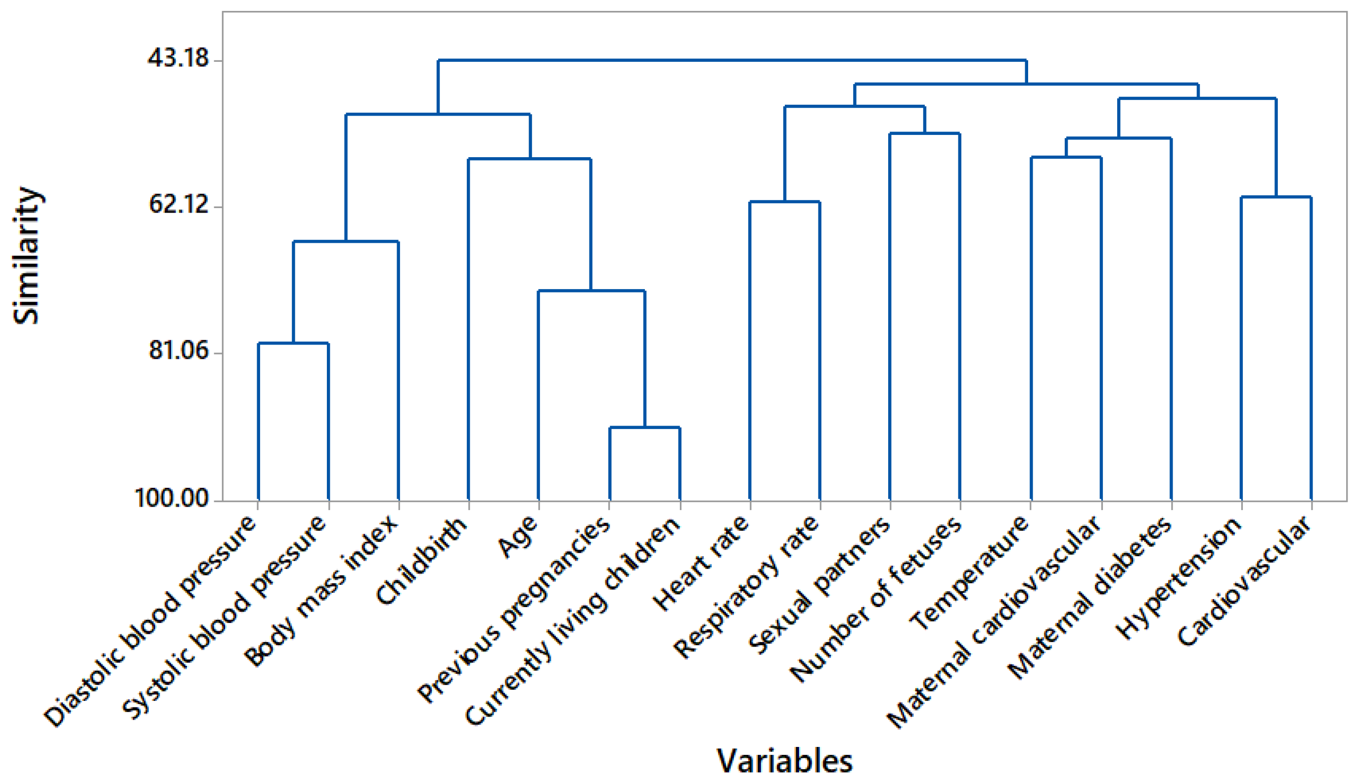
In Figure 1, a dendrogram is used to graphically observe the 16 features and their resemblance. Based on Figure 1, the state of the art and a description of each cluster is provided in Table 8. Previous and current live gestation are considered a single feature [25], as are heart rate and respiratory rate [26] and maternal cardiovascular and maternal diabetes [27]; thus, 13 characteristics are subtracted.

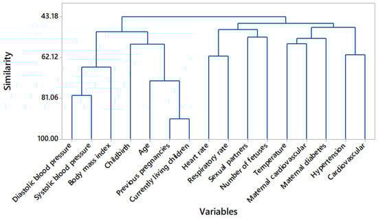
Figure 1. Dendrogram variable clustering.

Table 8. Amalgamation steps: description of each cluster.

Step	Number of Clusters	Similarity Level	Distance Level	Cluster Joined	New Cluster	Number of Objects in New Cluster
1	15	90.6540	0.18692	9 11	9	2
2	14	79.6475	0.40705	1 4	1	2
3	13	72.9477	0.54105	6 9	6	3
4	12	66.5169	0.66966	1 2	1	3
5	11	61.3923	0.77215	3 7	3	2
6	10	60.7389	0.78522	14 15	14	2
7	9	55.8924	0.88215	5 6	5	4
8	8	55.6662	0.88668	8 16	8	2
9	7	53.2323	0.93535	8 12	8	3
10	6	52.6070	0.94786	10 13	10	2
11	5	50.0891	0.99822	1 5	1	7
12	4	49.0337	1.01933	3 10	3	4
13	3	48.0947	1.03811	8 14	8	5
14	2	46.2200	1.07560	3 8	3	6
15	1	43.1843	1.13631	1 3	1	16

2.2.7. Recursive Feature Elimination

The recursive feature elimination (RFE) method works by recursively removing attributes and building a model from the remaining attributes. It uses precision metrics to rank the feature according to its importance.

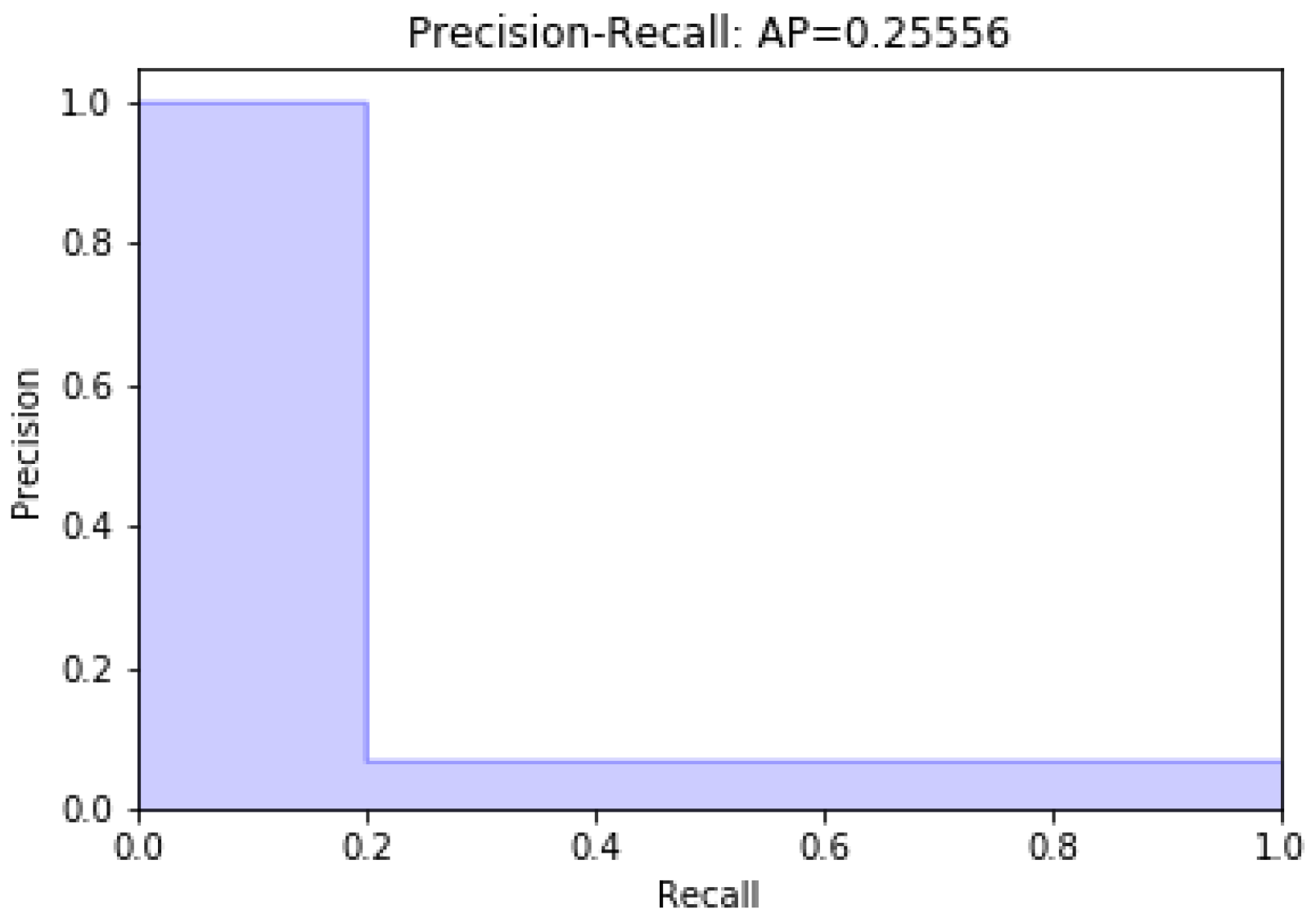
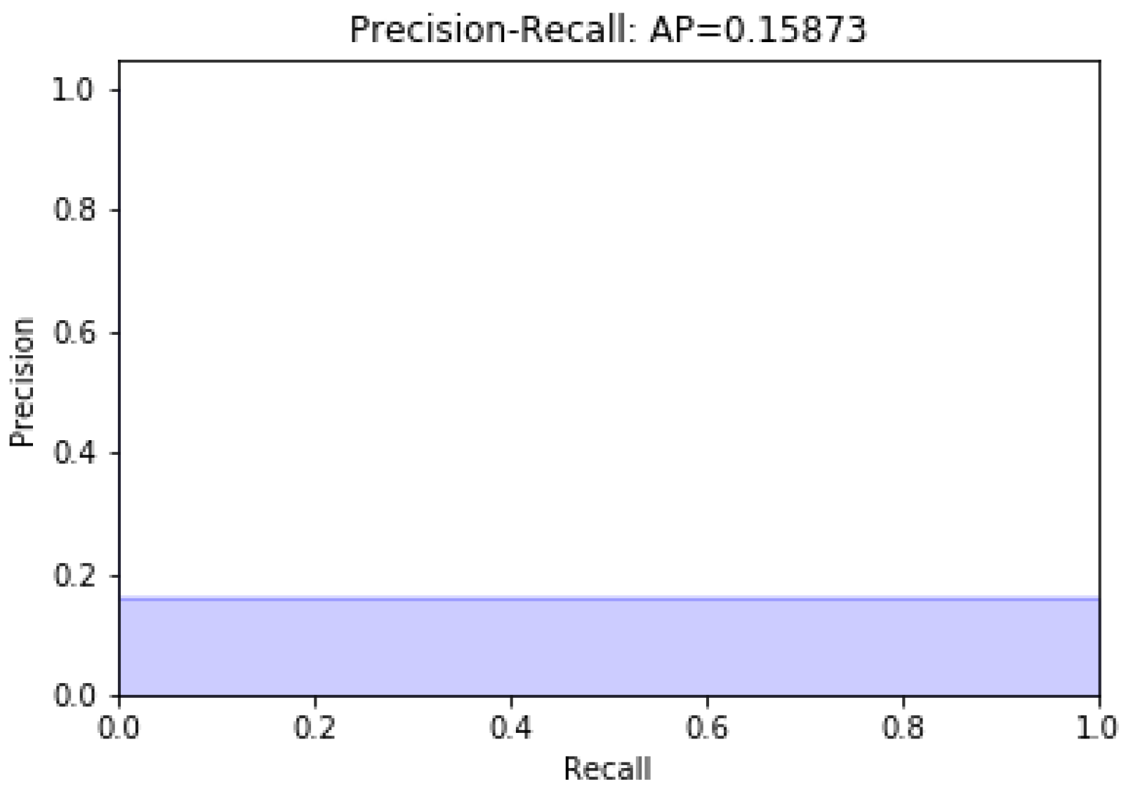
Data modeling with the remaining 13 characteristics was carried out; later, a variable was eliminated. Figure 2 and Figure 3 present unbalanced data modeling with SVM through precision–recall curves and the evaluation of all the features of the dataset, including discrepancy and when a variable is removed, respectively. The model’s performance was evaluated using recovery precision curves (precision–recall curves) through support vector machines for unbalanced classes on the advice of [28,29].

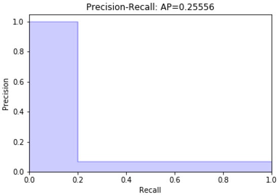
Figure 2. Modeling with the full dataset.

Figure 3. Modeling without diastolic pressure.

Table 9 summarizes the characteristics considered important following the RFE analysis, which are marked with True, and finally provides a total of eight features to be used when modeling the data.

Table 9. Recursive feature elimination and significant variables in the RFE analysis.

RFE Using SVM for Unbalanced Classes
True	Diastolic blood pressure
True	Body mass index
True	Heart rate
True	Systolic blood pressure
False	Childbirth
True	Age
False	Temperature
False	Previous pregnancies
False	Sexual partners
True	Maternal diabetes
True	Number of fetuses
True	Hypertension
False	Cardiovascular

2.3. Fuzzy Modeling

A rule-based model of the Takagi–Sugeno fuzzy type [30,31] is considered. It consists of a set of fuzzy rules, each describing a local input–output relationship in a linear form, as shown in Equation (9):

$$\begin{array}{c}\hfill R_i:\mathbf{If}X\mathrm{is}{C}_i\mathrm{Then}{\widehat{y}}_i={\theta }_{i}X\end{array}$$

(9)

where $R_i$ is the ith rule, and i goes from 1 to K, where K denotes the number of rules in the rule base. Two rules are established in this paper: when a pregnant woman is prone to some risk of preeclampsia and when she is not. $X=\left[x1, x2, \dots , x8\right]$ is the vector of the input variables, ${\theta }_i=[a_1, a_2, \dots , a_8]$ is the linear parameter vector [31], $C_i$ are the centroids or prototypes, and ${\widehat{y}}_i$ is the rule output, where $x_1$ is the diastolic blood pressure, $x_2$ is the heart rate, $x_3$ is the systolic blood pressure, $x_4$ is age, $x_5$ is maternal diabetes, $x_6$ is the number of fetuses, $x_7$ is hypertension, and $x_8$ is the body mass index.

The aggregated output of the model, $\widehat{y}\in Y$, ${\widehat{y}}_i$, is calculated by taking the weighted average of the rule consequents; see Equations (10) and (11) as follows:

$$\begin{array}{c}\hfill {\widehat{y}}_1={\beta }_1\left(X\right){\theta }_{1}X\end{array}$$

(10)

$$\begin{array}{c}\hfill {\widehat{y}}_2={\beta }_2\left(X\right){\theta }_{2}X\end{array}$$

(11)

where ${\beta }_i\left(X\right)$ is the degree of activation of the ith rule, which is shown in Equation (12) as follows:

$$\begin{array}{c}\hfill \beta i\left(X\right)=\prod _{j=1}^n{\mu }_{A_{ij}}\left(X_j\right),i=1, 2, \dots , K\end{array}$$

(12)

${\mu }_{A_{ij}}\left(X_j\right):\mathbb{R}\to \left[0,1\right]$ is the membership function of the fuzzy set $A_{ij}$ in the antecedent of $R_i$.

Table 10 defines the parameters for Rule 1 and Rule 2, identified using least squares weighted by the values of the degrees of activation of each fuzzy rule.

Table 10. Consequent parameters for Rules 1 and 2.

${\mathit{a}}_{\mathit{i}}$	Parameters Rule 1	Parameters Rule 2
$a_1$	$4.824\times {10}^{-17}$	−$9.215\times {10}^{-18}$
$a_2$	−$1.967\times {10}^{-17}$	−$1.658\times {10}^{-17}$
$a_3$	$1.42\times {10}^{-17}$	−$6.505\times {10}^{-19}$
$a_4$	$4.0115\times {10}^{-17}$	$3.577\times {10}^{-18}$
$a_5$	−$2.498\times {10}^{-15}$	−$1.915\times {10}^{-15}$
$a_6$	$1.179\times {10}^{-16}$	−$1.38\times {10}^{-15}$
$a_7$	−$6.947\times {10}^{-16}$	$4.839\times {10}^{-16}$
$a_8$	−$7.426\times {10}^{-17}$	$1.053\times {10}^{-16}$

A comparative study was carried out, examining the following four techniques: support vector machines, decision trees, random forests, and the T-S and FCM algorithms. There are two main ways to define the premises of fuzzy rules: one uses fuzzy grid partitioning with Gaussian, triangular, and trapezoid membership functions, and the other uses fuzzy clustering techniques, which were used in this work. Because it is an optimal algorithm in the search for multivariable patterns, which are useful for defining the premises of fuzzy rules, the T-S and FCM algorithm is briefly described [32]. The algorithm proposed here to predict preeclampsia in pregnant women considers two patterns: one for women at risk of suffering from preeclampsia and another for those not at risk of suffering from preeclampsia. Therefore, the model learned using the characteristics of women who did and did not suffer from preeclampsia. Only two cluster centers have the fuzzy model, with eight coordinates and eight consequent linear parameters.

FCM is based on the optimization of the target function c-means, as in Equation (13) as follows:

$$\begin{array}{c}\hfill J(Z;U,C)=\sum _i^c\sum _k^N{\left({\mu }_{ik}\right)}^m{∥z_k-c_i∥}^2\end{array}$$

(13)

where $Z=[z_1, z_2, \dots , z_N]$ is the data that must be classified

$$\begin{array}{c}\hfill U=\left[{\mu }_{ik}\in M_{fc}\right]\end{array}$$

(14)

It is a fuzzy Z-partition matrix,

$$\begin{array}{c}\hfill C=\left[c_1, c_2, \dots , c_c\right],c_i\in R^n\end{array}$$

(15)

The vector of centroids or prototypes is determined. It is la norma Euclidiana and is determined by the choice of matrix $B=\left[I\right]$ using Equation (16), as follows:

$$\begin{array}{c}\hfill D_{ik}^2={∥z_k-c_i∥}_B^2\end{array}$$

(16)

An exponent, m, determines the fuzziness of the resulting classes using Equation (17) as follows:

$$\begin{array}{c}\hfill m\in (1,\infty )\end{array}$$

(17)

Once the centers and fuzzy partition matrix have been obtained, defuzzification is carried out [33] to predict the new data, using Equations (18) and (19), as follows:

$$\begin{array}{c}\hfill {\mu }_{ik}={\displaystyle \frac{1}{{\sum }_{j=1}^c{(D_{ikB}/D_{jkB})}^{2/(m-1)}}};i=1, 2, \dots , c;k=1, 2, \dots , N\end{array}$$

(18)

$$\begin{array}{c}\hfill c_i={\displaystyle \frac{{\sum }_{k=1}^N{\left({\mu }_{ik}\right)}^m{z}_k}{{\sum }_{k=1}^N{\left({\mu }_{ik}\right)}^m}}\end{array}$$

(19)

Equation (19) yields a value for the centroids $c_i$ as the means of the data belonging to a specific class, where weights are the membership functions [31,32].

The fuzzy sets in the antecedent of the rules are obtained from the partition matrix U, whose $ik$th element ${\mu }_{ik}\in \left[0,1\right]$ is the membership degree of the data object $z_k$ in cluster i. The ith row of U contains a pointwise definition of a multidimensional fuzzy set. One-dimensional fuzzy sets $A_{ij}$ are obtained from the multidimensional fuzzy sets by projections onto the space of the input variables $X_j$ as in Equation (20) [31]:

$$\begin{array}{c}\hfill {\mu }_{A_{ij}}\left(X_{jk}\right)={\mathrm{pt}}_j\left({\mu }_{ik}\right)\end{array}$$

(20)

where $\mathrm{pt}$ is the pointwise projection operator [34]. The pointwise defined fuzzy sets $A_{ij}$ are then approximated using suitable parametric functions to compute ${\mu }_{A_{ij}}\left(X_{jk}\right)$ for any value of $X_j$.

The vector consequents $\left[{\theta }_i\right]$ of each T-S fuzzy rule are given using the least squares algorithm weighted by the degree of the firing of the fuzzy rule. The firing degree matrix ${\mathrm{\Gamma }}_i$ is defined, with the main diagonal of the elements being ${\mathrm{\Gamma }}_i=diag\left[{\mu }_{ik}\right]$.

The solution for the resulting least squares problem, $y={\theta }_{i}X+ϵ$, where $ϵ$ is the approximation error, is shown in Equation (21), for every fuzzy rule with $X_i^{\prime }={\mathrm{\Gamma }}_{i}X$. In the learning process, the vector $\left[y\right]$, conditioned with ones for PE cases and zeros for non-PE cases, is contained in the feature matrix $\left[X\right]$.

$$\begin{array}{c}\hfill {\theta }_i={\left[{\left(X^{\prime }\right)}^T{X}^{\prime }\right]}^{-1}{\left(X^{\prime }\right)}^{T}y\end{array}$$

(21)

3. Results

The values established by default were $i=2$, $m=3$, $maximum$$iterations=100$, and $minimal$$improvement=1\times {10}^{-5}$, where i is the number of rules to $C_i$, $maximum$ is the maximum number or iterations, $minimal$ is the minimal improvement, and fuzzy m is the exponent. For the learning of the two fuzzy rule patterns, the Matlab^® function $fcm\left(\right)$ was used, obtaining the premises of the rules results in the $centers$ and the fuzzy partition matrix, as shown in Table 11.

Table 11. Centers obtained in FCM for each variable.

Variable	Center 1	Center 2
Diastolic blood pressure	65.2358	62.3517
Heart rate	77.5245	76.1068
Systolic blood pressure	102.5317	98.5688
Age	24.5329	23.7132
Diabetes maternal	0.2740	0.2678
Number of fetuses	1.0194	1.0199
Hypertension	0.0377	0.03529
Body mass index	26.7199	25.9533

Table 12 shows the statistical measures for each of the features of the resulting dataset. This allows these features to be compared with the centers found in Table 11.

Table 12. Statistical measures for each feature.

Variable	Mean	St. Dev.	Minimum	Q1	Median	Q3	Maximum
Diastolic blood pressure	66.38	10.86	24	60	60	70	100
Heart rate	77.69	11.48	20	70	78	84	103
Systolic blood pressure	101.79	13.76	60	90	100	110	150
Age	24.316	7.059	14	18.75	24	28	43
Diabetes materna	0.2551	0.4382	0	0	0	1	1
Number of fetuses	1.102	0.3043	1	1	1	1	2
Hypertension	0.0408	0.1989	0	0	0	0	1
Body mass index	28.061	6.534	15.111	22.843	27.018	32.234	46.382

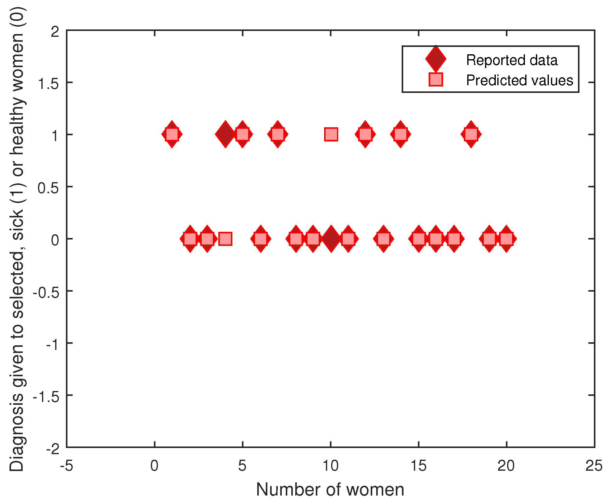
Figure 4 shows the evaluation of the learning performed for the T-S rule base and the premises with the centroids of the FCM algorithm. The 20 sample datasets selected contained 7 cases with hypertension versus 13 healthy cases; for these, there were two prediction errors.

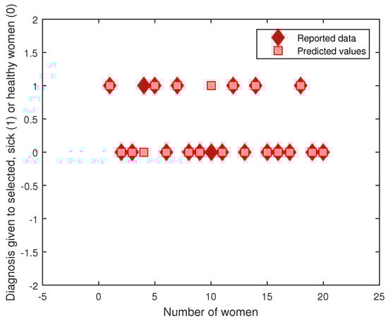
Figure 4. Predicted values vs. real measurements.

Evaluation

The precision is the ratio $tp/(tp+fp)$, where $tp$ is the number of true positives and $fp$ is the number of false positives. The precision is the ability of the classifier not to label as positive a sample that is negative. The recall is the ratio $tp/(tp+fn)$, where $tp$ is the number of true positives and $fn$ the number of false negatives, and the F-beta score is a weighted harmonic mean of the precision and recall [35].

Using these measures, a system that performs worse in the objective sense of informedness can appear to perform better under any of these commonly used measures. These standard measures have a significantly higher correlation with human judgments than the other proposed techniques [36]. Table 13 and Table 14 present the information obtained when evaluating the four proposed models without and with reducing dimensions, respectively. The evaluation was developed considering precision, recall, and the f-score to carry out a later evaluation using ROC and EER curves. A considerable increase in evaluation measures for fewer dimensions can be observed. A random undersampling technique [37] was used to adjust the class distribution of the dataset to eliminate the problem of unbalanced classes, therefore training the models with a total of 98 samples.

Table 13. Evaluation of the four selected models with 85 dimensions.

Model	Precision		Recall		F-Score		Sample Weight
To Sample Weight = None	Class 0	Class 1	Class 0	Class 1	Class 0	Class 1
SVM	0.6	0.3333	0.75	0.2	0.6666	0.25	None
	0.46666		0.5384		0.5384		Macro
	0.5384		0.5384		0.5384		Micro
	0.4974		0.5384		0.5064		Weighted
DT	0.6666	0.4285	0.5	0.6	0.5714	0.5	None
	0.5476		0.55		0.5357		Macro
	0.5384		0.5384		0.5384		Micro
	0.5750		0.5384		0.5439		Weighted
FCM	0.8333	0.5714	0.625	0.8	0.7142	0.6666	None
	0.7023		0.7125		0.6904		Macro
	0.6923		0.6923		0.6923		Micro
	0.7326		0.6923		0.6959		Weighted
RF	0.75	0.4444	0.375	0.8	0.5	0.5714	None
	0.5972		0.5875		0.5357		Macro
	0.53844		0.5384		0.5384		Micro
	0.6324		0.5384		0.5274		Weighted

Table 14. Evaluation of the four selected models with eight dimensions.

Model	Precision		Recall		F-Score		Sample Weight
To Sample Weight = None	Class 0	Class 1	Class 0	Class 1	Class 0	Class 1
SVM	0.6428	0.8333	0.9	0.5	0.75	0.625	None
	0.7380		0.7		0.6875		Macro
	0.7		0.7		0.7		Micro
	0.7380		0.7		0.6875		Weighted
DT	0.9166	0.3	0.825	0.5	0.8684	0.375	None
	0.6083		0.6625		0.6217		Macro
	0.7826		0.7826		0.78260		Micro
	0.7362		0.7826		0.7040		Weighted
FCM	0.8	0.8	0.8	0.8	0.8	0.8	None
	0.8		0.8		0.8000		Macro
	0.8		0.8		0.8000		Micro
	0.8		0.8		0.8000		Weighted
RF	0.805	0.75	0.7	0.8	0.7777	0.7181	None
	0.8125		0.8		0.7979		Macro
	0.8		0.8		0.8000		Micro
	0.7925		0.8		0.7979		Weighted

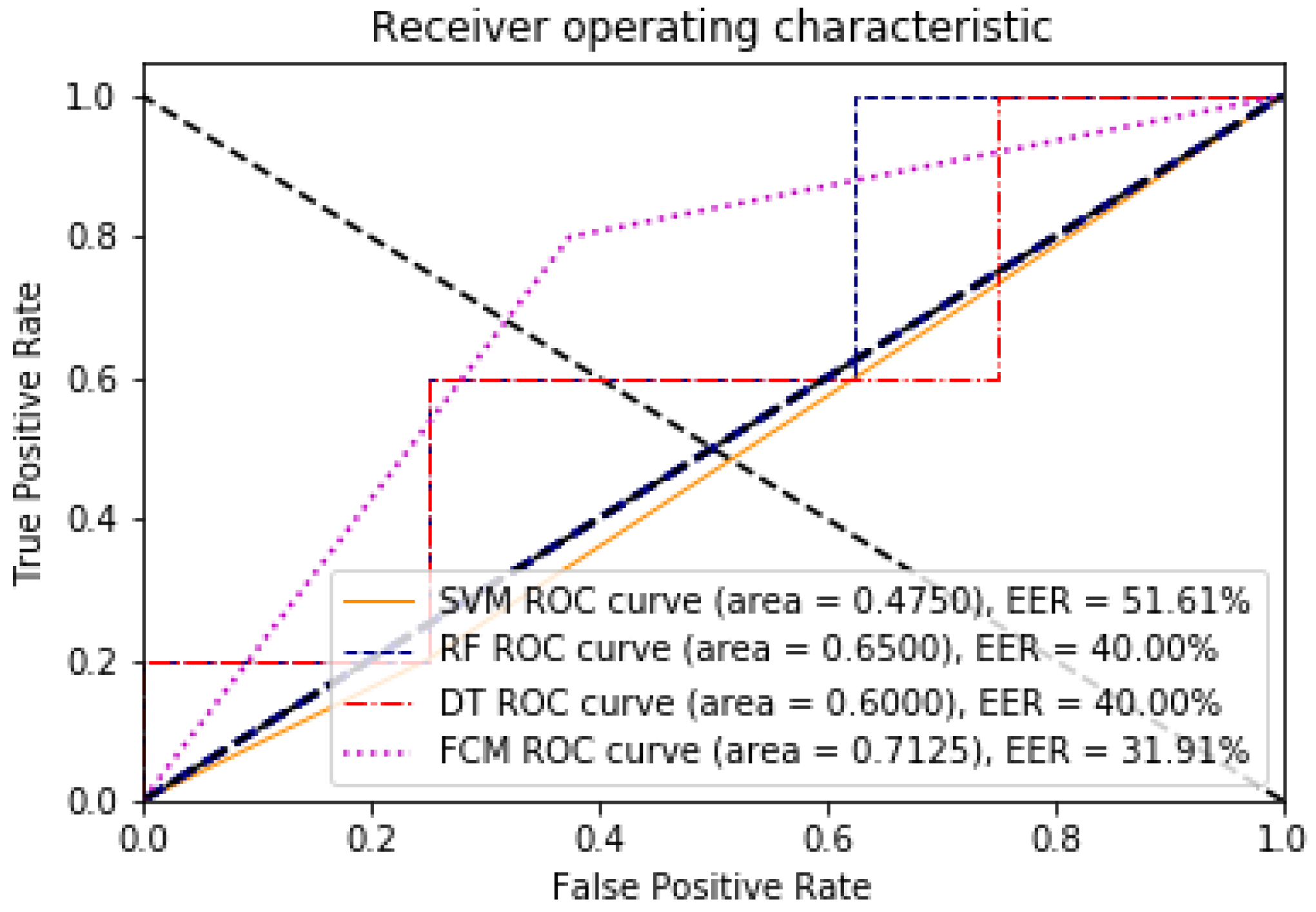
The area under the curve (AUC) is an indicator of the overall quality of a ROC curve. An ROC curve is a graphical representation of the sensitivity to specificity for a binary classification system as the discrimination threshold varies [38,39].

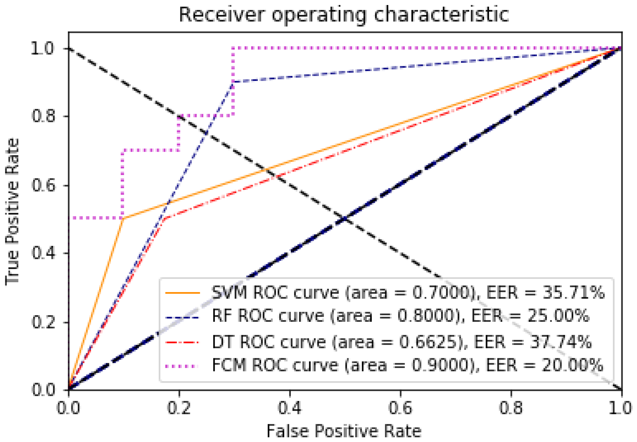
The point on the ROC curve that corresponds to the EER has an equal probability of wrongly classifying a positive or negative sample. This point is obtained by intersecting the ROC curve with a diagonal of the unit square [40]. A comparative analysis of the ROC and EER curves was performed to evaluate the performance of the models with and without dimensionality reduction. The evaluation of the algorithms with respect to these two measures can be seen in Figure 5 and Figure 6, for 85 features against the 8 found through the data discriminant; the improvement of the algorithms in their learning is remarkable.

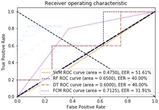
Figure 5. ROC and EER curves for the model with 85 dimensions, illustrating the trade-off between false positive and true positive rates.

Figure 6. ROC and EER curves for the model with eight dimensions, demonstrating the impact of dimensionality reduction on model performance.

4. Discussion

According to The American College of Obstetricians and Gynecologists [10], diastolic pressure, systolic pressure, and heart rate are representative variables in the diagnosis of PE [41,42]. There is some evidence of increased mortality among women with a history of hypertension during pregnancy [43]. Similarly, the overall risk of PE is higher for women with multiple pregnancies, nulliparity, and advanced maternal age, as mentioned in [44].

In [45], the authors establish that there is a relationship between pre-pregnancy body mass index and the risk of severe and mild PE, as well as the risk of severe and mild transient pregnancy hypertension. It is well known that there is a relationship between parents with type 2 diabetes and the possible inheritance of diabetes by their descendants [46,47]; it is clear that there is a strong hereditary component to the disease.

In addition, type 1 and 2 diabetes, gestational diabetes, and polycystic ovarian syndrome are all well-established risk factors for pregnancy-induced hypertension [48]. Therefore, based on the statistical and pattern recognition analyses performed, the maternal hypertension variable is accepted as an important characteristic in the prediction of hypertension in pregnancy and its derivatives.

In [13], a fuzzy intelligent system implemented via wearable devices is proposed for patients with preeclampsia. This system works using five descriptive variables, namely systolic pressure, diastolic pressure, proteinuria, age, and weight, to detect preeclampsia and diabetes. However, since the clinical records of women in Hidalgo do not include information on the occurrence of proteinuria, statistics were used to determine representative variables. As a result, eight significant variables (diastolic pressure, body mass index, heart rate, systolic pressure, age, maternal diabetes, number of fetuses, and hypertension) are presented, which agree with the previous literature.

5. Conclusions

The data obtained through the SSEH allowed us to carry out a dimensional reduction analysis to contrast our work with the results established in the literature. Initially, we had 85 dimensions, which were subjected to data pre-processing to find those that were not significant to modeling PE. Based on a study in which the authors reduced the characteristic variables, as reported in the literature, we successfully reduced the dimensionality to only eight critical variables through clamp transformation, correlation coefficients, and a multicollinearity analysis. The correlation coefficient allowed for the elimination of more characteristics by finding 15 constant variables, followed by a multicollinearity analysis through which four variables were reduced by a value of $\widehat{{\alpha }_i}>5$.

The eight variables obtained resulted in a fuzzy T-S model that showed favorable classification results on real data in comparison to other models in the literature. The FCM clearly finds and identifies patterns in biological data. Likewise, some data centers are closely distanced; FCM instead allows for the identification of the type of cluster to which the input vector belongs using features with greater variation.

The present results show an approximate value of $0.8$ for the EER in the FCM analysis with eight dimensions for the evaluation of the precision and recall rate when the worst scenario is shown; this information is consistent with the result obtained in EER (20%). However, by evaluating with respect to the ROC curve, we obtain an approximate value of 90% in the prediction of hypertensive disorders in pregnancy. A lower EER indicates a better balance between these two types of errors, thus reflecting a more accurate model. Having both EER evaluation and ROC curves together is beneficial because EER provides a concise summary of accuracy at the threshold where false positive and false negative rates are equal, simplifying model comparison at a specific point. Another advantage of FCM is that even without reducing dimensions and balancing, it is capable of a higher degree of learning and classification than other algorithms. When all the dimensions were used, the learning rate was 71.25 % without undersampling; therefore, this allows us to say that a fuzzy approach expands the possibilities of using biological data in binary classification.

References

- Steegers, E.A.; Von Dadelszen, P.; Duvekot, J.J.; Pijnenborg, R. Pre-eclampsia. Lancet 2010, 376, 631–644. [Google Scholar] [CrossRef]
- Davey, D.A.; MacGillivray, I. The classification and definition of the hypertensive disorders of pregnancy. Am. J. Obstet. Gynecol. 1988, 158, 892–898. [Google Scholar] [CrossRef] [PubMed]
- Özsezer, G.; Mermer, G. Prevention of Maternal Mortality: Prediction of Health Risks of Pregnancy with Machine Learning Models. 2023. Available online: https://www.researchgate.net/publication/368845364_Prevention_of_Maternal_Mortality_Prediction_of_Health_Risks_of_Pregnancy_with_Machine_Learning_Models (accessed on 1 July 2024).
- Raza, A.; Siddiqui, H.U.R.; Munir, K.; Almutairi, M.; Rustam, F.; Ashraf, I. Ensemble learning-based feature engineering to analyze maternal health during pregnancy and health risk prediction. PLoS ONE 2022, 17, e0276525. [Google Scholar] [CrossRef]
- Ramla, M.; Sangeetha, S.; Nickolas, S. Fetal health state monitoring using decision tree classifier from cardiotocography measurements. In Proceedings of the 2018 Second International Conference on Intelligent Computing and Control Systems (ICICCS), Madurai, India, 14–15 June 2018; pp. 1799–1803. [Google Scholar]
- Irfan, M.; Basuki, S.; Azhar, Y. Giving more insight for automatic risk prediction during pregnancy with interpretable machine learning. Bull. Electr. Eng. Inform. 2021, 10, 1621–1633. [Google Scholar] [CrossRef]
- Alam, M.S.B.; Patwary, M.J.; Hassan, M. Birth mode prediction using bagging ensemble classifier: A case study of bangladesh. In Proceedings of the 2021 International Conference on Information and Communication Technology for Sustainable Development (ICICT4SD), Dhaka, Bangladesh, 27–28 February 2021; pp. 95–99. [Google Scholar]
- Haldar, N.A.H.; Khan, F.A.; Ali, A.; Abbas, H. Arrhythmia classification using Mahalanobis distance based improved Fuzzy C-Means clustering for mobile health monitoring systems. Neurocomputing 2017, 220, 221–235. [Google Scholar] [CrossRef]
- Neocleous, C.K.; Anastasopoulos, P.; Nikolaides, K.H.; Schizas, C.N.; Neokleous, K.C. Neural networks to estimate the risk for preeclampsia occurrence. In Proceedings of the 2009 International Joint Conference on Neural Networks, Atlanta, GA, USA, 14–19 June 2009; pp. 2221–2225. [Google Scholar]
- American College of Obstetricians and Gynecologists. Hypertension in pregnancy. Report of the American College of Obstetricians and Gynecologists’ task force on hypertension in pregnancy. Obstet. Gynecol. 2013, 122, 1122. [Google Scholar]
- Moreira, M.W.; Rodrigues, J.J.; Oliveira, A.M.; Ramos, R.F.; Saleem, K. A preeclampsia diagnosis approach using Bayesian networks. In Proceedings of the 2016 IEEE International Conference on Communications (ICC), Kuala Lumpur, Malaysia, 22–27 May 2016; pp. 1–5. [Google Scholar]
- Moreira, M.W.; Rodrigues, J.J.; Oliveira, A.M.; Saleem, K.; Neto, A.J.V. Predicting hypertensive disorders in high-risk pregnancy using the random forest approach. In Proceedings of the 2017 IEEE International Conference on Communications (ICC), Paris, France, 21–25 May 2017; pp. 1–5. [Google Scholar]
- Espinilla, M.; Medina, J.; García-Fernández, Á.L.; Campaña, S.; Londoño, J. Fuzzy intelligent system for patients with preeclampsia in wearable devices. Mob. Inf. Syst. 2017, 2017, 7838464. [Google Scholar] [CrossRef]
- Babuška, R. Fuzzy Modeling for Control; Springer Science & Business Media: Berlin/Heidelberg, Germany, 1998; Volume 12. [Google Scholar]
- Velikova, M.; van Scheltinga, J.T.; Lucas, P.J.; Spaanderman, M. Exploiting causal functional relationships in Bayesian network modelling for personalised healthcare. Int. J. Approx. Reason. 2014, 55, 59–73. [Google Scholar] [CrossRef]
- Tejera, E.; Jose areias, M.; Rodrigues, A.; Ramoa, A.; Manuel nieto villar, J.; Rebelo, I. Artificial neural network for normal, hypertensive, and preeclamptic pregnancy classification using maternal heart rate variability indexes. J. -Matern.-Fetal Neonatal Med. 2011, 24, 1147–1151. [Google Scholar] [CrossRef] [PubMed]
- Kelleher, J.D.; Mac Namee, B.; D’arcy, A. Fundamentals of Machine Learning for Predictive Data Analytics: Algorithms, Worked Examples, and Case Studies; MIT Press: Cambridge, MA, USA, 2015. [Google Scholar]
- Garcia Asuero, A.; Sayago, A.; González, G. The Correlation Coefficient: An Overview. Crit. Rev. Anal. Chem. 2006, 36, 41–59. [Google Scholar] [CrossRef]
- Mansfield, E.R.; Helms, B.P. Detecting multicollinearity. Am. Stat. 1982, 36, 158–160. [Google Scholar]
- Wold, S.; Esbensen, K.; Geladi, P. Principal component analysis. Chemom. Intell. Lab. Syst. 1987, 2, 37–52. [Google Scholar] [CrossRef]
- Breiman, L. Random forests. Mach. Learn. 2001, 45, 5–32. [Google Scholar] [CrossRef]
- Khalilia, M.; Chakraborty, S.; Popescu, M. Predicting disease risks from highly imbalanced data using random forest. BMC Med. Inform. Decis. Mak. 2011, 11, 51. [Google Scholar] [CrossRef] [PubMed]
- Han, H.; Guo, X.; Yu, H. Variable selection using mean decrease accuracy and mean decrease gini based on random forest. In Proceedings of the 2016 7th IEEE International Conference on Software Engineering and Service Science (ICSESS), Beijing, China, 26–28 August 2016; pp. 219–224. [Google Scholar]
- Hastie, T.; Tibshirani, R.; Friedman, J. The Elements of Statistical Learning: Data Mining, Inference, and Prediction; Springer Science & Business Media: Berlin/Heidelberg, Germany, 2009. [Google Scholar]
- Altfeld, S.; Handler, A.; Burton, D.; Berman, L. Wantedness of pregnancy and prenatal health behaviors. Women Health 1998, 26, 29–43. [Google Scholar] [CrossRef]
- Mehlsen, J.; Pagh, K.; Nielsen, J.; Sestoft, L.; Nielsen, S. Heart rate response to breathing: Dependency upon breathing pattern. Clin. Physiol. 1987, 7, 115–124. [Google Scholar] [CrossRef] [PubMed]
- Selvin, E.; Marinopoulos, S.; Berkenblit, G.; Rami, T.; Brancati, F.L.; Powe, N.R.; Golden, S.H. Meta-analysis: Glycosylated hemoglobin and cardiovascular disease in diabetes mellitus. Ann. Intern. Med. 2004, 141, 421–431. [Google Scholar] [CrossRef]
- Maldonado, S.; Weber, R.; Famili, F. Feature selection for high-dimensional class-imbalanced data sets using Support Vector Machines. Inf. Sci. 2014, 286, 228–246. [Google Scholar] [CrossRef]
- Maldonado, S.; Weber, R. A wrapper method for feature selection using support vector machines. Inf. Sci. 2009, 179, 2208–2217. [Google Scholar] [CrossRef]
- Takagi, T.; Sugeno, M. Fuzzy identification of systems and its applications to modeling and control. IEEE Trans. Syst. Man Cybern. 1985, SMC-15, 116–132. [Google Scholar] [CrossRef]
- Setnes, M.; Babuska, R.; Verbruggen, H.B. Rule-based modeling: Precision and transparency. IEEE Trans. Syst. Man Cybern. Part C (Appl. Rev.) 1998, 28, 165–169. [Google Scholar] [CrossRef]
- Díez, J.L.; Navarro, J.L.; Sala, A. Algoritmos de agrupamiento en la identificación de modelos borrosos. Rev. Iberoam. de Automática e Informática Ind. 2010, 1, 32–41. [Google Scholar]
- Babuška, R. Fuzzy Systems, Modeling and Identification; Delft University of Technology, Department of Electrical Engineering Control Laboratory, Mekelweg: Delft, The Netherlands, 1996; Volume 4. [Google Scholar]
- Kruse, R.; Gebhardt, J.E.; Klowon, F. Foundations of Fuzzy Systems; John Wiley & Sons, Inc.: Hoboken, NJ, USA, 1994. [Google Scholar]
- Powers, D. Evaluation: From Precision, Recall and F-Factor to ROC, Informedness, Markedness & Correlation. Mach. Learn. Technol. 2008, 2. [Google Scholar]
- Melamed, I.D.; Green, R.; Turian, J.P. Precision and recall of machine translation. In Proceedings of the HLT-NAACL, Stroudsburg, PA, USA, 31 May 2003; pp. 61–63. [Google Scholar]
- Yap, B.W.; Rani, K.A.; Rahman, H.A.A.; Fong, S.; Khairudin, Z.; Abdullah, N.N. An application of oversampling, undersampling, bagging and boosting in handling imbalanced datasets. In Proceedings of the First International Conference on Advanced Data and Information Engineering (DaEng-2013); Springer: Berlin/Heidelberg, Germany, 2014; pp. 13–22. [Google Scholar]
- Carter, J.V.; Pan, J.; Rai, S.N.; Galandiuk, S. ROC-ing along: Evaluation and interpretation of receiver operating characteristic curves. Surgery 2016, 159, 1638–1645. [Google Scholar] [CrossRef] [PubMed]
- Al-Nima, R.R.O.; Dlay, S.S.; Woo, W.L.; Chambers, J.A. A novel biometric approach to generate ROC curve from the probabilistic neural network. In Proceedings of the 2016 24th Signal Processing and Communication Application Conference (SIU), IEEE, Zonguldak, Turkey, 16–19 May 2016; pp. 141–144. [Google Scholar]
- Davis, J.; Goadrich, M. The relationship between Precision-Recall and ROC curves. In Proceedings of the 23rd International Conference on Machine Learning, ACM, Pittsburgh, PA, USA, 25–29 June 2006; pp. 233–240. [Google Scholar]
- Program, National High Blood Pressure Education. Report of the national high blood pressure education program working group on high blood pressure in pregnancy. Am. J. Obstet. Gynecol. 2000, 183, s1–s22. [Google Scholar] [CrossRef]
- Caritis, S.; Sibai, B.; Hauth, J.; Lindheimer, M.D.; Klebanoff, M.; Thom, E.; VanDorsten, P.; Landon, M.; Paul, R.; Miodovnik, M.; et al. Low-dose aspirin to prevent preeclampsia in women at high risk. N. Engl. J. Med. 1998, 338, 701–705. [Google Scholar] [CrossRef] [PubMed]
- Sjónsdóttir, L.; Arngrimsson, R.; Geirsson, R.T.; Slgvaldason, H.; Slgfússon, N. Death rates from ischemic heart disease in women with a history of hypertension in pregnancy. Acta Obstet. Gynecol. Scand. 1995, 74, 772–776. [Google Scholar] [CrossRef]
- Savitz, D.A.; Zhang, J. Pregnancy-induced hypertension in North Carolina, 1988 and 1989. Am. J. Public Health 1992, 82, 675–679. [Google Scholar] [CrossRef]
- Bodnar, L.M.; Catov, J.M.; Klebanoff, M.A.; Ness, R.B.; Roberts, J.M. Prepregnancy body mass index and the occurrence of severe hypertensive disorders of pregnancy. Epidemiology 2007, 18, 234–239. [Google Scholar] [CrossRef]
- Kaufman, F.R. Type 2 diabetes mellitus in children and youth: A new epidemic. J. Pediatr. Endocrinol. Metab. 2002, 15, 737–744. [Google Scholar] [CrossRef]
- Arslanian, S.A. Type 2 diabetes mellitus in children: Pathophysiology and risk factors. J. Pediatr. Endocrinol. Metab. 2000, 13, 1385–1394. [Google Scholar] [CrossRef] [PubMed]
- Carty, D.M.; Delles, C.; Dominiczak, A.F. Novel biomarkers for predicting preeclampsia. Trends Cardiovasc. Med. 2008, 18, 186–194. [Google Scholar] [CrossRef] [PubMed]
Disclaimer/Publisher’s Note: The statements, opinions and data contained in all publications are solely those of the individual author(s) and contributor(s) and not of MDPI and/or the editor(s). MDPI and/or the editor(s) disclaim responsibility for any injury to people or property resulting from any ideas, methods, instructions or products referred to in the content. |
© 2024 by the authors. Licensee MDPI, Basel, Switzerland. This article is an open access article distributed under the terms and conditions of the Creative Commons Attribution (CC BY) license (https://creativecommons.org/licenses/by/4.0/).