Converting Tessellations into Graphs: From Voronoi Tessellations to Complete Graphs

Abstract

A mathematical procedure enabling the transformation of an arbitrary tessellation of a surface into a bi-colored, complete graph is introduced. Polygons constituting the tessellation are represented by vertices of the graphs. Vertices of the graphs are connected by two kinds of links/edges, namely, by a green link, when polygons have the same number of sides, and by a red link, when the polygons have a different number of sides. This procedure gives rise to a semi-transitive, complete, bi-colored Ramsey graph. The Ramsey semi-transitive number was established as $R_{trans}\left(3,3\right)=5$ Shannon entropies of the tessellation and graphs are introduced. Ramsey graphs emerging from random Voronoi and Poisson Line tessellations were investigated. The limits $\zeta =\underset{N\to \infty }{\lim }{\displaystyle \frac{N_g}{N_r}}$, where N is the total number of green and red seeds, $N_g$ and $N_r$, were found $\zeta =$ 0.272 ± 0.001 (Voronoi) and $\zeta =$ 0.47 ± 0.02 (Poisson Line). The Shannon Entropy for the random Voronoi tessellation was calculated as $S=$ 1.690 ± 0.001 and for the Poisson line tessellation as S = 1.265 ± 0.015. The main contribution of the paper is the calculation of the Shannon entropy of the random point process and the establishment of the new bi-colored Ramsey graph on top of the tessellations.

1. Introduction

A tessellation (also called “tiling”) is covering a surface with a pattern of flat shapes so that there are no overlaps or gaps [1,2,3]. Tessellations are important for physics [4], materials science [5] and engineering [6]. Theory of tessellations plays a key role in the explaining of the structure of quasi-crystals [7,8,9,10]. In our paper we propose the mathematical procedure enabling converting the tessellation into bi-colored complete graphs [11,12,13]. Thus, the methods of graph theory became applicable to the analysis of tessellations. Results supplied by the Ramsey theory become useful for the study of tiles [14,15,16].

Thus, Chartland et al. showed that for every two integers p and q with 2 ≤ p < q, there exists a graph with a red-blue coloring possessing a maximal Ramsey chain of length p and a maximum Ramsey chain of length q, whereas for every positive integer k, there exists a graph with a red-blue coloring possessing at least k maximal Ramsey chains of distinct lengths with prescribed conditions [17].

Transformation of the tiles into graphs enables the calculation of the Shannon entropy of the emerging graphs [18,19,20]. General meaning of the Ramsey theory may be formulated as follows: “complete chaos is impossible”. In a system of given size ordered patterns inevitably emerge. The natural measure of “orderliness” is a Shannon/Voronoi entropy, which is a standard tool to analyze the Voronoi tessellation. We will exemplify the suggested transformation with Voronoi tessellations converted into bi-colored, complete graphs and calculation of the corresponding Shannon/Voronoi entropy [21,22,23,24]. Such analysis has not been done in the literature before. We also applied the introduced transformation to the analysis of the Poisson line tessellations. In the next sections we will present the results of the entropy calculation for the Voronoi and Poisson line tessellations and statistical limits of the involved bi-colored graphs. First, we will present the mathematical method and the computational results. We will further discuss these results in the discussion section.

2. Methods

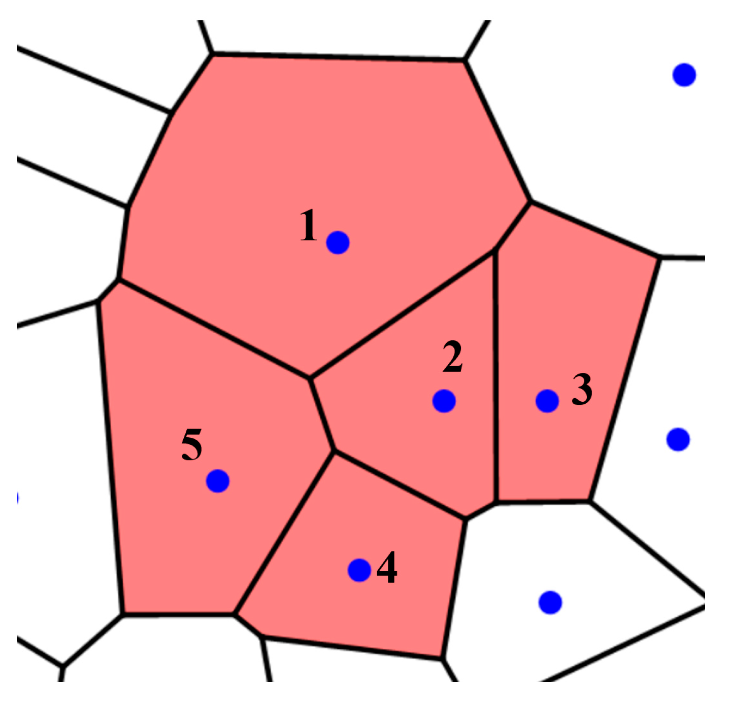
2.1. Converting of Tessellations into Bi-Colored, Complete Graphs

Consider the 2D tessellation shown in Figure 1. The tessellation is built from five polygons, numbered $\left\{1,2\dots 5\right\}$. The tessellation is constructed by two triangles, numbered “4” and “5”, two quadrangles, numbered “1” and “2”, and a pentagon, numbered “3”. The polygons form a rectangle, which is the fundamental region for the suggested tessellation. We introduce the following procedure enabling converting the tessellation into a complete, bi-colored graph. Polygons are represented by vertices of the graphs, as shown in Figure 2. Vertices of the graphs are connected by two kinds of links/edges, namely, green links when polygons have the same number of sides, and red links otherwise, i. e., when the polygons have a different number of sides. In other words, green links connect homomorphic polygons while red links connect heteromorphic polygons.

The bi-colored graph depicted in Figure 2 emerges from the tessellation shown in Figure 1. It is emphasized that the introduced procedure gives rise to bi-colored complete graphs for any tessellation. Note that the “green relation” between the vertices of the graph is transitive, whereas the “red relation” is not. Consider three polygons labeled “a”, “b”, and “c”. If pairs of polygons “a” and “b” and “b” and “c” have the same number of sides, the polygons “a” and “c” necessarily have the same number of sides. Hence, green links represent a transitive relation between the vertices of the graph. This is not true for the red links. Consider three polygons labeled “a”, “b” and “c”. Assume, that pairs of polygons “a” and “b” and “b” and “c” have a different number of sides. It is still possible that polygons “a” and “c” have the same or different number of sides thus making the red relation non-transitive. This observation is of primary importance for the analysis of the addressed graphs. These graphs, emerging from 2D tessellations, may be labeled as semi-transitive graphs.

Let us take a close look at a graph, shown in Figure 2. Triangles “135”, “234”, “235”, and “134” are monochromatic (red ones). It turns out that at least one monochromatic triangle will necessarily appear within the complete bi-colored graph, comprising five vertices, when at least one of the links, represents the transitive relation. We proved it with a method of “brute force” by searching through all possible graphs, comprising five vertices in which at least one of the links is transitive. Regrettably, the method of brute force remains the only method for establishing the Ramsey numbers.

Let us introduce the semi-transitive Ramsey number ${\mathit{R}}_{\mathit{t}\mathit{r}\mathit{a}\mathit{n}\mathit{s}}\left(\mathit{m},\mathit{n}\right),$which is defined as a positive integer, for which every green-red edge coloring of the complete graph on ${\mathit{R}}_{\mathit{t}\mathit{r}\mathit{a}\mathit{n}\mathit{s}}\left(\mathit{m},\mathit{n}\right)$ vertices necessarily contains a green clique on m vertices or a red clique on n vertices, when the colored links represent the transitive relation between the vertices. We demonstrated that ${\mathit{R}}_{\mathit{t}\mathit{r}\mathit{a}\mathit{n}\mathit{s}}\left(\mathbf{3},\mathbf{3}\right)=\mathbf{5}$. Recall, that for the complete bi-colored graphs, which do not contain transitive links $\mathit{R}\left(\mathbf{3},\mathbf{3}\right)=\mathbf{6}$.

It is possible to create a semi-transitive bi-colored complete graph, containing four vertices in which no monochromatic triangle is present. This graph is shown in Figure 3. Again, green links represent transitive relations between vertices, and red links represent non-transitive relations.

Arbitrary monohedral tiling necessarily gives rise to the mono-colored completely transitive graph.

2.2. Shannon Entropy of the Introduced Graphs and Tessellations

Quantification of the “orderliness” of the tessellation shown in Figure 1 may be carried out with the Shannon measure/entropy. The Shannon entropy (denoted S) of a given set tessellation is introduced with Equation (1) [10,18,19]:

$$S=-{{\displaystyle \sum }}_i{P}_{i}ln{P}_i$$

(1)

where $P_i$ is the fraction of the polygons possessing i edges in the tiling. The summation in Equation (1) is performed from i = 3 (the smallest possible polygon, a triangle) to the largest coordination number of the polygon, e.g., for a hexagon, the largest value of i is 6. Tessellation presented in Figure 1 contains two triangles, two quadrangles, and one pentagon, thus, the Shannon Entropy of tessellation is calculated with Equation (1) as $S=-\left({\displaystyle \frac{2}{5}}ln{\displaystyle \frac{2}{5}}+{\displaystyle \frac{2}{5}}ln{\displaystyle \frac{2}{5}}+{\displaystyle \frac{1}{5}}ln{\displaystyle \frac{1}{5}}\right)\cong 1.065$. This measure may be also introduced for bi-colored graphs, such as that shown in Figure 2 and Figure 3 [20]. Shannon entropies of the graphs in introduced by Equations (2) and (3) (compare with the classical definition of the Shannon entropy defined by Equation (1):

$${\mathit{S}}_{\mathit{g}}=-{{\displaystyle \sum }}_{\mathit{n}}{\mathit{P}}_{\mathit{n}\mathit{g}}\mathit{l}\mathit{n}{\mathit{P}}_{\mathit{n}\mathit{g}}, \mathit{n}\ge \mathbf{3}$$

(2)

$${\mathit{S}}_{\mathit{r}}=-{{\displaystyle \sum }}_{\mathit{i}}{\mathit{P}}_{\mathit{i}\mathit{r}}\mathit{l}\mathit{n}{\mathit{P}}_{\mathit{i}\mathit{r}},\ge \mathbf{3},$$

(3)

where ${\mathit{P}}_{\mathit{n}\mathit{g}}$ is the fraction of monochromatic convex polygons with n green edges, and${\mathit{P}}_{\mathit{i}\mathit{r}}$ is the fraction of monochromatic convex polygons with i red edges in a complete bi-colored graph. Sampling of polygons is carried out separately from the green and red subsets of convex polygons. Thus, a pair of Shannon entropies $\left({\mathit{S}}_{\mathit{g}},{\mathit{S}}_{\mathit{r}}\right)$ corresponds to any bi- or mono-colored complete graph. The introduced Shannon entropies $\left({\mathit{S}}_{\mathit{g}},{\mathit{S}}_{\mathit{r}}\right)$ are completely defined by the given distribution of monochromatic polygons in the addressed graph. Let us illustrate this idea with the complete graph, presented in Figure 2.

For this graph, we establish ${\mathit{P}}_{\mathit{n}\mathit{g}}=\mathbf{0}$ for any $\mathit{n}\ge \mathbf{3}$ (no monochromatic green polygons appear in the graph); ${\mathit{P}}_{\mathit{i}\mathit{r}}=\mathbf{1}$ for $\mathit{i}=\mathbf{3}$; ${\mathit{P}}_{\mathit{i}\mathbf{3}}=\mathbf{0}$ for any $\mathit{i}>\mathbf{3}$ (only red triangles are present in the graph). Thus, according to Equations (2) and (3), the both of the Shannon entropies ${\mathit{S}}_{\mathit{g}}$ and ${\mathit{S}}_{\mathit{r}}$ equal zero. Now we introduce the following notation:${\mathit{S}}_{\mathit{r}}=\mathbf{0}$, ${\mathit{S}}_{\mathit{g}}=\tilde{\mathbf{0}}$ [20]. This notation enables distinguishing between zero Shannon entropies emerging from the situations when ${\mathit{P}}_{\mathit{n}}=\mathbf{0}$ and ${\mathit{P}}_{\mathit{n}}=\mathbf{1}$ appearing in Equations (2) and (3) take place; namely $\mathit{S}=\mathbf{0}$ when ${\mathit{P}}_{\mathit{n}}=\mathbf{1}$for a given $\mathit{n}\ge \mathbf{3}$, and $\mathit{S}=\tilde{\mathbf{0}}$ when ${\mathit{P}}_{\mathit{n}}=\mathbf{0}$ for any $\mathit{n}\ge \mathbf{3}$. For the graph, presented in Figure 2 we establish.

$$\left({\mathit{S}}_{\mathit{g}},{\mathit{S}}_{\mathit{r}}\right)=\left(\tilde{\mathbf{0}},\mathbf{0}\right)$$

(4)

For the complete bi-colored graph, depicted in Figure 3, we establish: $\left({\mathit{S}}_{\mathit{g}},{\mathit{S}}_{\mathit{r}}\right)=\left(\tilde{\mathbf{0}}, \tilde{\mathbf{0}}\right)$. The tiling shown in Figure 1 is edge-to-edge tiling, however, the introduced converting of the tiling may be also introduced for the tiling, which is not edge-to-edge.

2.3. Transformation of the Voronoi Tessellation into the Bi-Colored Complete Graph

A Voronoi tessellation or diagram of an infinite plane is a partitioning of the plane into regions based on the distance to a specified discrete set of points (called seeds, nuclei, or generators) [21,22]. Voronoi tessellations, also known as Voronoi diagrams, are a type of tiling in which the plane is subdivided into n polygonal cells enclosing a portion of the plane that is closest to each of n points [21,22]. The Voronoi pattern can be found in nature and engineering, including architecture, materials, and computer science [23,24,25,26,27,28]. Voronoi tessellations were exploited recently for the analysis of biological images [29]. Voronoi diagrams were introduced as early as 1644 by René Descartes and were used by Dirichlet in the study of positive quadratic forms [24].

Consider the random Voronoi tessellation depicted in Figure 4. The random seeds were generated with the Mersenne twister. Calculations were carried out with Wolfram Mathematics.

Now we imply the procedure enabling converting of the Voronoi tessellation into the bi-colored complete, graph, introduced in Section 2.1. We connect seeds generating the tessellation (shown with blue points in Figure 4) with two kinds of colored links: green and red.

Now we exploit the suggested procedure enabling the transformation of the Voronoi tessellation into the graph, namely: green links connect polygons with an equal number of sides, whereas red links connect polygons with different numbers of sides. The procedure gives rise to the semi-transitive graph, as explained in detail in Section 2.1. Let us illustrate this procedure, with the Voronoi polygons, shown in Figure 5.

Polygon 1 in Figure 5 and Figure 6 is octagon; polygons “2”, “3” and “4” are pentagons, polygon “6” is hexagon. Figure 6 depicts bi-colored complete graph, emerging from polygons $\left\{1,\dots 5\right\}$.

Recall that the semi-transitive Ramsey number was established in Section 2.1 as ${\mathit{R}}_{\mathit{t}\mathit{r}\mathit{a}\mathit{n}\mathit{s}}\left(\mathbf{3},\mathbf{3}\right)=\mathbf{5}$. Indeed, the triangles “234”, “135”, “125” and “145” appearing in Figure 6 are mono-colored.

As is seen from Figure 6, the red polygons include 3 triangles and 3 quadrangles. Thus, the Shannon Entropy of the red graph is supplied by Equation (3) as: ${\mathit{S}}_{\mathit{r}}=-\left({\displaystyle \frac{\mathbf{3}}{\mathbf{6}}}\mathit{l}\mathit{n}{\displaystyle \frac{\mathbf{3}}{\mathbf{6}}}+{\displaystyle \frac{\mathbf{3}}{\mathbf{6}}}\mathit{l}\mathit{n}{\displaystyle \frac{\mathbf{3}}{\mathbf{6}}}\right)\approx \mathbf{0.6931}$ green graph consists of one triangle only, which necessarily implies a zero Shannon entropy value ${\mathit{S}}_{\mathit{g}}=\mathbf{0}$. Thus, the pair of the Shannon entropies for the graph shown in Figure 6 is $\left({\mathit{S}}_{\mathit{g}},{\mathit{S}}_{\mathit{r}}\right)=\left(\mathbf{0}, \mathbf{0.6931}\right)$.

3. Methods

3.1. Statistics of Voronoi Tessellation

The Voronoi tessellation of a random set of point at an infinite plane is of particular interest. It is believed that the entropy of the Voronoi tessellation given by Equation (1) referred to as the “Voronoi entropy,” S_v, can be used as a measure of orderliness of the [10]. For a perfectly ordered set of points on a plane, ${\mathit{S}}_{\mathit{V}}=\mathbf{0}$, while for a randomly distributed points the experimental values close to ${\mathit{S}}_{\mathit{V}}=\mathbf{1.7}$ have been reported [24].

For many characteristics of the Voronoi tessellation of a random set including the statistical distribution of the relative number of polygons with the given number of edges, P_n, there is no known analytical formula in the closed form. Instead, Monte Carlo and other simulation methods are used to obtain these parameters from numerical experiments. While analytical solutions have been suggested by Hayen and Quine for n = 3 [30], and Calca for the general case of any integer n ≥ 3 [31], these solutions are in the integral form, which requires numerical integration. Some of these numerical results are summarized in

Table 1. Probability distribution of polygons for Voronoi tessellation of a set of random points from literature sources [33].

Authors	Crain, 1978 [34]	Hinde & Miles, 1980 [32]	Kumar & Kurtz, 1993 [35]	Calka, 2003 [31]	Tanemura, 2003 [36]	Brakke, 2005 [37]
Number of polygons, N	57,000	2,000,000	650,000	Monte Carlo numerical integration was used	10,000,000	208,969,210
P3	0.011	0.01131	0.011	0.01124	0.01125	0.01125
P4	0.1078	0.1071	0.1071	0.106838	0.10685	0.10683
P5	0.2594	0.2591	0.26	0.25946	0.25946	0.25945
P6	0.2952	0.2944	0.294	0.29473	0.29473	0.29471
P7	0.1984	0.1991	0.199	0.19877	0.19877	0.1988
P8	0.0896	0.0902	0.09	0.0897	0.0897	0.09012
P9	0.0296	0.0295	0.03	0.0295	0.0295	0.02964
P10	0.00751	0.00743	0.007	0	0	0.00745
P11	0.00142	0.00149	0.0015	0	0	0.00148
P12	0.000175	0.00025	0.00023	0	0	0.00024
P13	0.000053	0.00003	0.00004	0	0	0.00003
SV	1.68927	1.69066	1.68902	1.64087	1.64092	1.69031
ζ	0.273072	0.272438	0.272718	0.27251	0.272515	0.272729

. As far as accuracy, Calca [32] estimated an error of 10⁻⁶ for n = 3, 4, 10⁻⁵ for n = 5, 6, 7, and 10⁻⁴ for n = 8, 9 [31]. The Voronoi entropy of the tessellation is calculated from Equation (1).

The number of green links (i.e., links between polygons of the same number of edges) is given by the sum of the squares of the numbers of such polygons.

$$N_g={\displaystyle \frac{N^2}{2}}{{\displaystyle \sum }}_{n=3}^{\infty }{\left(P_n\right)}^2$$

(5)

where N is the total number of polygons. The number of red links (i.e., links between polygons of different number of edges) is given by

$$N_r={\displaystyle \frac{N^2}{2}}\left[1-{{\displaystyle \sum }}_{n=3}^{\infty }{\left(P_n\right)}^2\right]$$

(6)

Consequently, the ratio of the two numbers is given by

$$\zeta ={\displaystyle \frac{N_g}{N_r}}={\displaystyle \frac{{{\displaystyle \sum }}_{n=3}^{\infty }{\left(P_n\right)}^2}{1-{{\displaystyle \sum }}_{n=3}^{\infty }{\left(P_n\right)}^2}}$$

(7)

In the matrix form, for vector ${\mathrm{P}}^{\mathrm{T}}=\left(P_3,P_4,\dots P_N\right)$, the number of links is given as the trace of a matrix $\mathrm{P}·{\mathrm{P}}^{\mathrm{T}}$, whose diagonal contains squared probabilities $P_n^2$

$$N_g={\displaystyle \frac{N^2}{2}}\mathrm{Tr}\left(\mathrm{P}·{\mathrm{P}}^{\mathrm{T}}\right)$$

(8)

$$N_r={\displaystyle \frac{N^2}{2}}\left[1-\mathrm{Tr}\left(\mathrm{P}·{\mathrm{P}}^{\mathrm{T}}\right)\right]$$

(9)

$$\zeta ={\displaystyle \frac{\mathrm{Tr}\left(\mathrm{P}·{\mathrm{P}}^{\mathrm{T}}\right)}{1-\mathrm{Tr}\left(\mathrm{P}·{\mathrm{P}}^{\mathrm{T}}\right)}}$$

(10)

The results are presented in Table 1 for the literature data [31,32,33,34,35,36,37]. Note that in Table 1, we use results numerical simulation. It is very difficult to obtain theoretical values of the frequency distribution parameters.

Certain statistical features of random Voronoi tessellations have been reported. Thus, theoretical studies suggest that the distribution of the number of sides is provided by a generalized three-parameter Gamma (3P) distribution [32,33]. The Lewis law states that for a random pattern, there is a linear relationship between the number of edges and the mean area of polygons [38]. The Desch law states a linear relation between the perimeter of polygons and the number of their edges [39]. For a Voronoi cell that neighbors another n-sided cell, the Aboav–Weaire law relates the average number of sides m_n of as ${\mathit{m}}_{\mathit{n}}=\mathit{a}+{\displaystyle \frac{\mathit{b}}{\mathit{n}}}$, where a and b are constant [38].

We therefore conclude that based on the literature data, the ratio of green-to-red links (transitive homomorphic to non-transitive heteromorphic relations) in a random Voronoi set is within the interval 0.2724 < ζ < 0.2731 while the value of the Voronoi Entropy is in the interval 1.689 < S_v < 1.691 (excluding values calculated from Refs. [31,36] as insufficient number of polygons, 3 < n < 9, were considered). This is an important result, because previously it was believed that the value of the Voronoi entropy of the random point process can reach S_v < 1.71 [24,40].

3.2. Statistics of Poisson Line Tessellation

Another type of random tessellation is the Poisson line tessellation, which is obtained by the tessellation of an infinite plane by randomly placed and oriented straight lines. The statistics of such tessellation was obtained by Tanner [41] and is given by P₃ = 0.355066, P₄ = 0.381466, P₅ = 0.1895, P₆ = 0.05870, P₇ = 0.01275, P₈ = 0.002082, P₉ = 0.0002712, P₁₀ = 0.000018, P₁₁ = 0.0000028, P₁₂ = 0.0000004 [41]. The values for P₃ and P₄ are calculated from theoretical considerations, while for higher number of edges in polygons the values are obtained from numerical experiments [41,42]. The Equations (1) and (7) immediately yield the Shannon entropy of S = 1.2779 and the ratio ζ = 0.4516.

3.3. Numerical Simulation

3.3.1. Random Voronoi Tessellation

To investigate the dependency of the ratio ζ upon the number of polygons, we conducted a numerical simulation was conducted for up to N = 6000 polygons.

The dependency of the ratio of the number of green and red links denoted ${\mathit{N}}_{\mathit{g}}$ and ${\mathit{N}}_{\mathit{r}}$ correspondingly on the number of polygons N is presented in Figure 7a. The yellow line indicates the limit $\mathit{\zeta }=$ 0.272 ± 0.001. The value is consistent with the value 0.2724 < ζ < 0.2731 obtained from the distribution calculations found in the literature, as discussed in the preceding section. The envelope orange curves are drawn in accordance with the expression $\tilde{\mathit{\delta }}\left(\mathit{N}\right)=\mathbf{0.272}\left(\mathbf{1}\pm {\displaystyle \frac{\mathbf{2}}{\sqrt{\mathit{N}}}}\right)$ (see Figure 7a).

We also calculated the Shannon entropy of the tessellation (the Voronoi entropy) as a function of the number of seeds ${\mathit{S}}_{\mathit{V}}\left(\mathit{N}\right)$ calculated with Equation (1) (Figure 7b). The limiting value was close to S_V = 1.69. This value is close to the limiting value calculated for the Shannon Entropy of the random Voronoi tessellations using results reported by other groups, 1.689 < S_V < 1.691 [40], as discussed in the preceding section.

3.3.2. Random Polygons Produced by Straight Lines (Poisson Line Tessellation)

In many situations, random tessellations are not generated by randomly placed seed points, but by randomly placed straight lines oriented under arbitrary angles. Such a situation is typical in materials science when micro/nanofibers are placed under arbitrary angles forming a network-like structure, for which Voronoi entropy is sometimes applied [43].

The lines were generated with the origin at random points and with a random orientation. The number of lines from N_L = 10 to N_L = 70, with the increment of 10, were tested (Figure 8a). For every number of lines five simulations were conducted. The distribution of the number of edges in polygons (Figure 8b) is consistent with the literature results, as discussed above (P₃ = 0.3550, P₄ = 0.3814, P₅ = 0.1895, P₆ = 0.0587, P₇ = 0.0127, P₈ = 0.0002).

The dependency of the ratio of the number of green and red links ${\mathit{N}}_{\mathit{g}}$/${\mathit{N}}_{\mathit{r}}$ on the number of polygons N is presented in Figure 9a. demonstrating the limiting value of $\mathit{\zeta }=$ 0.47 ± 0.02. The value is consistent with the literature value ζ = 0.4516, as discussed in the preceding section. The dependency of the Shannon entropy on the number of seeds $\mathit{S}\left(\mathit{N}\right)$ is shown in Figure 9b. The limiting value was close to S = 1.265 ± 0.015. This value is close to the limiting value calculated for the Shannon Entropy of the Poisson Line tessellations calculated from the data reported by other groups, S = 1.2779, as discussed in the preceding section.

4. Discussion

Tessellations (or tiles) are widespread in mathematics, engineering and arts [3,4,25,26,27,28,29]. We introduce the mathematical procedure enabling transformation of the arbitrary tessellation into complete, bi-colored, semi-transitive graph. Thus, application of the Ramsey theory becomes possible for the analysis of tessellations. We illustrate the idea with the analysis of Voronoi tessellations. In our future investigations we plan to apply the suggested mathematical framework for the analysis of a diversity of natural and engineering patterns.

The bi-colored graph obtained by the proposed procedure has a number of remarkable properties. For an infinite plane tessellation, the number of edges scales as N². We define a sub-graph built from the green links only as a “green sub-graph”, and a grant built of red links only, in turn, as a “red sub-graph”. The quantity of green sub-graphs depends on the number of types of polygons present and the number of edges in each graph is equal to ζP_nN²/2 for n-th type of green polygons. The red sub-graph is only one and the number of its edges is (1 − ζ)N²/2. The red sub-graph is a connected graph (a connected graph is graph that is connected in the sense of a topological space, i.e., there is a path from any point to any other point in the graph). The green sub-graphs, are also connected ones.

The degree distribution, clustering coefficients, and features related to percolation and resilience can further be calculated [44,45]. Introduced mathematical technique is well expected to be useful for the analysis of properties of composite materials [46,47].

We have developed a semi-transitive Ramsey bi-colored graph using the tessellation of a plane. The work can be expanded for further analysis of Ramsey graphs.

The nearest application of the suggested theory is related to the analysis of polycrystalline materials [48]. The Voronoi network, addressed in Section 2.2 contains geometric information about spatial arrangement of the atomic centers, seen as the seeds of Voronoi tessellation [48]. The polygons, thus, represent the grains of the emerging polycrystalline structure [48,49]. The distribution of grains/polygons, in turn, impact the properties of the entire polycrystalline body [49,50]. Another application of the introduced mathematical procedure enabling converting of tessellations into graphs is related to modern gauge field theories [4].

5. Conclusions

Arbitrary tessellation of a plane may be transformed into the complete, bi-colored graph, with the following mathematical technique: polygons are represented by the vertices of the graph, which are connected by two kinds of links/edges. Green links connect the vertices representing polygons with equal number of sides, while red links are between the vertices representing polygons with a different number of sides. The green links constitute a transitive relation between the vertices, while the red links constitute the relation which is not transitive. Consequently, the procedure gives rise for a semi-transitive, bi-colored, complete graph. The Ramsey number for such a graph $R_{trans}\left(3,3\right)=5$was established. This means, that the monochromatic triangle will necessarily appear within the graph built of five vertices. The Ramsey number was established by searching through all possible graphs, containing five vertices. The degree of order of the original tessellation is quantified with the Shannon Entropy. The degree of order of the emerging graph is quantified with a pair of the Shannon entropies, supplying the averaged probability to find the monochromatic polygon within the given graph.

We illustrate the suggested technique with the transformation of the Voronoi and Poisson Line tessellations into the semi-transitive, bi-colored, complete graphs. We investigated the graphs emerging from the random distribution of the seed points on the plane. We calculated the limit $\zeta =$ 0.272 ± 0.001 emerging from the random Voronoi tessellation and $\zeta =$ 0.47 ± 0.02 emerging from the random Poisson Line tessellation. The limit value of the Shannon Entropy for the random Voronoi tessellation was calculated as $S=$ 1.690 ± 0.001 and for the Poisson line tessellation as S = 1.265 ± 0.015.

References

1. Coxeter, H.S.M. Chapter IV, Two-Dimensional Crystallography. In Introduction to Geometry; John Wiley and Sons: New York, NY, USA, 1969; pp. 50–65. [Google Scholar]
2. Coxeter, H.S.M. Chapter IV, Tessellations and Honeycombs. In Regular Polytopes; Dover Publications: New York, NY, USA, 1973; pp. 58–73. [Google Scholar]
3. Fulton, C. Tessellations. Am. Math. Mon. 1992, 99, 442–445. [Google Scholar] [CrossRef]
4. He, Y.H.; van Loon, M. Gauge theories, tessellations & Riemann surfaces. J. High Energy Phys. 2014, 2014, 53. [Google Scholar]
5. Wu, S.; Sun, Y. Tessellating tiny tetrahedrons. Science 2018, 362, 1354–1355. [Google Scholar] [CrossRef] [PubMed]
6. Meloni, M.; Zhang, Q.; Pak, J.; Bilore, M.N.; Ma, R.; Ballegaard, E.; Lee, D.; Cai, J. Designing origami tessellations composed of quadrilateral meshes and degree-4 vertices for engineering applications. Autom. Constr. 2022, 142, 104482. [Google Scholar] [CrossRef]
7. Shechtman, D.; Blech, I.; Gratias, D.; Cahn, J.W. Metallic phase with long-range orientational order and no translational symmetry. Phys. Rev. Lett. 1984, 53, 1951–1953. [Google Scholar] [CrossRef]
8. Collins, L.; Witte, T.; Silverman, R.; Green, D.B.; Gomes, K.K. Imaging quasiperiodic electronic states in a synthetic Penrose tiling. Nat. Commun. 2017, 8, 15961. [Google Scholar] [CrossRef] [PubMed]
9. Bursill, L.; Lin, P.J. Penrose tiling observed in a quasi-crystal. Nature 1985, 316, 50–51. [Google Scholar] [CrossRef]
10. Bormashenko, E.; Legchenkova, I.; Frenkel, M.; Shvalb, N.; Shoval, S. Voronoi Entropy vs. Continuous Measure of Symmetry of the Penrose Tiling: Part I. Analysis of the Voronoi Diagrams. Symmetry 2021, 13, 1659. [Google Scholar]
11. Wilson, R.J. Introduction to Graph Theory, 4th ed.; Addison Wesley Longman Limited: Harlow, UK, 1996; pp. 8–21. [Google Scholar]
12. Trudeau, R.J. Introduction to Graph Theory (Corrected, Enlarged Republication ed.); Dover Pub.: New York, NY, USA, 1993; pp. 19–64. [Google Scholar]
13. Li, Y.; Lin, Q. Elementary Methods of the Graph Theory; Applied Mathematical Sciences; Springer: Cham, Switzerland, 2020; pp. 3–44. [Google Scholar]
14. Katz, M.; Reimann, J. An Introduction to Ramsey Theory: Fast Functions, Infinity, and Metamathematics; Student Mathematical Library; American Mathematical Society: Providence, RI, USA, 2018; Volume 87, pp. 1–34. [Google Scholar]
15. Graham, R.L.; Spencer, J.H. Ramsey Theory. Sci. Am. 1990, 7, 112–117. [Google Scholar] [CrossRef]
16. Graham, R.; Butler, S. Rudiments of Ramsey Theory, 2nd ed.; American Mathematical Society: Providence, RI, USA, 2015; pp. 7–46. [Google Scholar]
17. Chartrand, G.; Chatterjee, R.; Zhang, P. Ramsey chains in graphs. Electron. J. Math. 2023, 6, 1–14. [Google Scholar] [CrossRef]
18. Shannon, C.E. A Mathematical Theory of Communication. Bell Syst. Tech. J. 1948, 27, 379–423. [Google Scholar] [CrossRef]
19. Ben-Naim, A. Entropy, Shannon’s Measure of Information and Boltzmann’s H-Theorem. Entropy 2017, 19, 48. [Google Scholar] [CrossRef]
20. Frenkel, M.; Shoval, S.; Bormashenko, E. Shannon Entropy of Ramsey Graphs with up to Six Vertices. Entropy 2023, 25, 1427. [Google Scholar] [CrossRef] [PubMed]
21. Voronoi, G. Nouvelles applications des paramètres continus à la théorie des formes quadratiques. Deuxième mémoire. Recherches sur les paralléloèdres primitifs. Reine Angew. Math. 1908, 134, 198–287. [Google Scholar] [CrossRef]
22. Okabe, A.; Boots, B.; Sugihara, K. Spatial Tessellations Concepts and Applications of Voronoi Diagrams; John Wiley & Sons: Chichester, UK, 2000. [Google Scholar]
23. Barthélemy, M. Spatial networks. Phys. Rep. 2011, 499, 1–101. [Google Scholar] [CrossRef]
24. Bormashenko, E.; Frenkel, M.; Vilk, A.; Legchenkova, I.; Fedorets, A.A.; Aktaev, N.E.; Dombrovsky, L.A.; Nosonovsky, M. Characterization of Self-Assembled 2D Patterns with Voronoi Entropy. Entropy 2018, 20, 956. [Google Scholar] [CrossRef] [PubMed]
25. Habib, F.; Megahed, N.A.; Badawy, N.; Shahda, M.M. D4G framework: A novel Voronoi diagram classification for decoding natural geometrics to enhance the built environment. Archit. Sci. Rev. 2024, 1–28. [Google Scholar] [CrossRef]
26. Angelucci, G.; Mollaioli, F. Voronoi-like Grid Systems for Tall Buildings. Front. Built Environ. 2018, 4, 78. [Google Scholar] [CrossRef]
27. Zhu, S.; Borodin, E.; Jivkov, A.P. Discrete modelling of continuous dynamic recrystallisation by modified Metropolis algorithm. Comput. Mater. Sci. 2024, 234, 112804. [Google Scholar] [CrossRef]
28. Bolshakov, P.; Kharin, N.; Agathonov, A.; Halinin, E.; Sachenkov, O. Extension of the Voronoi Diagram Algorithm to Orthotropic Space for Material Structural Design. Biomimetics 2024, 9, 185. [Google Scholar] [CrossRef]
29. Jungck, J.R.; Pelsmajer, M.J.; Chappel, C.; Taylor, D. The Re-Visioning Frontier of Biological Image Analysis with Graph Theory, Computational Geometry, and Spatial Statistics. Mathematics 2021, 9, 2726. [Google Scholar] [CrossRef]
30. Hayen, A.; Quine, M. The proportion of triangles in a Poisson-Voronoi tessellation of the plane. Adv. Appl. Prob. (SGSA) 2002, 32, 67–74. [Google Scholar] [CrossRef]
31. Calka, P. The explicit expression of the distribution of the number of sides of the typical Poisson Voronoi cell. Adv. Appl. Probab. 2003, 35, 863–870. [Google Scholar] [CrossRef]
32. Hinde, A.L.; Miles, R.E. Monte Carlo estimates of the distributions of the random polygons of the Voronoi tessellation with respect to a Poisson process. J. Stat. Comput. Simul. 1980, 10, 205–223. [Google Scholar] [CrossRef]
33. Suárez-Plasencia, L.; Herrera-Macías, J.A.; Legón-Pérez, C.M.; Socorro-Lanes, R.; Rojas, O.; Sosa-Gómez, G. Analysis of the Number of Sides of Voronoi Polygons in PassPoint. In Computer Science and Health Engineering in Health Services. COMPSE 2020, 4th EAI Virtual International Conference, Lecture Notes of the Institute for Computer Sciences, Social Informatics and Telecommunications Engineering; Marmolejo-Saucedo, J.A., Vasant, P., Litvinchev, I., Rodriguez-Aguilar, R., Martinez-Rios, F., Eds.; Springer: Cham, Switzerland, 2021; Volume 359, pp. 184–200. [Google Scholar] [CrossRef]
34. Crain, I.K. The Monte Carlo generation of random polygons. Comput. Geosci. 1978, 4, 131–141. [Google Scholar] [CrossRef]
35. Kumar, S.; Kurtz, S.K. Properties of a two-dimensional Poisson-Voronoi tessellation: A Monte-Carlo study. Mater. Charact. 1993, 31, 55–68. [Google Scholar] [CrossRef]
36. Tanemura, M. Statistical distributions of Poisson Voronoi cells in two and three dimensions. FORMA-TOKYO 2003, 18, 221–247. [Google Scholar]
37. Brakke, K.A. 200,000,000 Random Voronoi Polygons; Dept. Math. Sciences, Susquehanna University: Selinsgrove, PA, USA, 2015; pp. 1–11. [Google Scholar]
38. Chiu, S.N. Aboav-Weaire’s and Lewis’ laws—A review. Mater. Charact. 1995, 34, 149–165. [Google Scholar] [CrossRef]
39. Saraiva, J.; Pina, P.; Bandeira, L.; Antunes, J. Polygonal networks on the surface of Mars; applicability of Lewis, Desch and Aboav–Weaire laws. Phil. Mag. Lett. 2009, 89, 185–193. [Google Scholar] [CrossRef]
40. Limaye, A.V.; Narhe, R.D.; Dhote, A.M.; Ogale, S.B. Evidence for convective effects in breath figure formation on volatile fluid surfaces. Phys. Rev. Lett. 1996, 76, 3762–3765. [Google Scholar] [CrossRef]
41. Tanner, J.C. Polygons Formed by Random Lines in a Plane: Some Further Results. J. Appl. Probab. 1983, 20, 778–787. [Google Scholar] [CrossRef]
42. Calka, P. Precise Formulae for the Distributions of the Principal Geometric Characteristics of the Typical Cells of a Two-Dimensional Poisson-Voronoi Tessellation and a Poisson Line Process. Adv. Appl. Probab. 2003, 35, 551–562. [Google Scholar] [CrossRef]
43. Botnar, A.; Novokov, O.; Korepanov, O. Crystallization Control of Anionic Thiacalixarenes on Silicon Surface Coated with Cationic Poly(ethyleneimine). ACS Appl. Mater. Interfaces, 2024; submitted. [Google Scholar]
44. Bormashenko, E.; Fedorets, A.A.; Frenkel, M.; Dombrovsky, L.A.; Nosonovsky, M. Clustering and self-organization in small-scale natural and artificial systems. Phil. Trans. R. Soc. A 2020, 378, 20190443. [Google Scholar] [CrossRef]
45. Nosonovsky, M.; Roy, P. Scaling in Colloidal and Biological Networks. Entropy 2020, 22, 622. [Google Scholar] [CrossRef]
46. Wang, W.; Wang, H.; Fei, S.; Wang, H.; Dong, H.; Ke, Y. Generation of random fiber distributions in fiber reinforced composites based on Delaunay triangulation. Mater. Des. 2021, 206, 109812. [Google Scholar] [CrossRef]
47. Pan, Y.; Iorg, L.; Pelegri, A. Numerical generation of a random chopped fiber composite RVE and its elastic properties. Compos. Sci. Technol. 2008, 68, 2792–2798. [Google Scholar] [CrossRef]
48. Anikeenko, A.V.; Gavrilova, M.L.; Medvedev, N.N. The coloring of the voronoi network: Investigation of structural heterogeneity in the packings of spheres. Jpn. J. Indust. Appl. Math. 2005, 22, 151–165. [Google Scholar] [CrossRef]
49. Li, M.; Xi, T. Topological and atomic scale characterization of grain boundary networks in polycrystalline and nanocrystalline materials. Prog. Mater. Sci. 2011, 56, 864–899. [Google Scholar] [CrossRef]
50. Pan, S.P.; Feng, S.D.; Qiao, J.W.; Wang, W.M.; Qin, J.U. Crystallization pathways of liquid-bcc transition for a model iron by fast quenching. Sci. Rep. 2015, 5, 16956. [Google Scholar] [CrossRef]
Figure 1. Tessellation of the plane with five polygons is depicted. Polygons “4” and “5” are triangles; polygons “1” and “2” are quadrangles; polygon “3” is a pentagon.
Mathematics 12 02426 g001
Figure 2. A complete bi-colored graph emerging from the tessellation shown in Figure 1. The vertices of the graph represent polygons, shown in Figure 1. If polygons have the same number of sides/edges, the vertices of the graph are connected by a green link; if polygons have a different number of sides/edges the vertices are connected by a red link.
Mathematics 12 02426 g002
Figure 3. A semi-transitive graph built of four vertices is depicted. Green links represent transitive relations between the vertices; red links relations between the vertices which are non-transitive. No monochromatic triangle is recognized in the graph.
Mathematics 12 02426 g003
Figure 4. Voronoi tessellation generated by a set of N = 30 points. Seeds are shown with blue points. The considered polygons are colored with deep tomato red.
Mathematics 12 02426 g004
Figure 5. Five Voronoi polygons extracted from the Voronoi tessellation, shown in Figure 4. Blue points depict the seeds/generators. The considered polygons are colored with deep tomato red. The polygons are numbered   { 1 5 } .
Mathematics 12 02426 g005
Figure 6. Bi-colored complete graphs generated by polygons { 1 , 5 } . Polygon 1 is octagon; polygons “2”, “3” and “4” are pentagons, and polygon “6” is hexagon.
Mathematics 12 02426 g006
Figure 7. (a) The ratio of the number of green and red links and (b) the Voronoi entropy depending on the number of seeds N. Orange curves in inset (a) are the envelope functions δ ˜ ( N ) = 0.272 ( 1 ± 2 N ) . Orange straight line in inset (b) depicts the asymptotic value of the Voronoi entropy.
Mathematics 12 02426 g007
Figure 8. The (a) Poisson line tessellation and (b) the distribution of the number of polygons (a) for NL = 50 lines.
Mathematics 12 02426 g008
Figure 9. The convergence of the (a) ratio the number of green–to-red links and (b) Shannon entropy as a function of the number of polygons in Poisson line tessellation.
Mathematics 12 02426 g009