Abstract
Financial time series data are characterized by non-linearity, non-stationarity, and stochastic complexity, so predicting such data presents a significant challenge. This paper proposes a novel hybrid model for financial forecasting based on CEEMDAN-SE and ARIMA- CNN-LSTM. With the help of the CEEMDAN-SE method, the original data are decomposed into several IMFs and reconstructed via sample entropy into a lower-complexity stationary high-frequency component and a low-frequency component. The high-frequency component is predicted by the ARIMA statistical forecasting model, while the low-frequency component is predicted by a neural network model combining CNN and LSTM. Compared to some classical prediction models, our algorithm exhibits superior performance in terms of three evaluation indexes, namely, RMSE, MAE, and MAPE, effectively enhancing model accuracy while reducing computational overhead.
MSC:
68T07
1. Introduction
Financial time series, as a quintessential form of temporal data, are crucial components of financial markets, reflecting the current economic conditions of a market. Moreover, as an investment approach marked by high risks and high returns, predicting their future trends and mitigating investment risks have become pressing issues. However, this kind of data is characterized by high volatility, non-linearity, and non-stationarity, so determining how to predict these kinds of trends is very challenging. Traditional time series methods employ statistical forecasting techniques, such as the Autoregressive Integrated Moving Average (ARIMA) model, which perform well for stationary linear data but fail to capture the dynamics of non-stationary multivariate time series. With the gradual development of artificial intelligence technology, machine learning methods have started to be applied to the prediction of non-stationary financial data, including decision tree forecasting [1], SVM prediction [2], neural network forecasting [3], gradient boosting [4], reinforcement learning prediction [5], and deep learning prediction [6].
Furthermore, determining how to reduce the complexity of time series data has become a new research direction. Huang, Shen, and Long et al. [7] innovatively proposed the Empirical Mode Decomposition (EMD) method, which decomposes non-linear and non-stationary time series signals into a stationary linear intrinsic mode function (IMF) and significantly reduces the complexity of the original sequence. However, EMD suffers from issues such as decomposition residuals and mode mixing. Wu and Huang [8] then introduced the Ensemble Empirical Mode Decomposition (EEMD) method, which addresses mode mixing by adding white noise, but the handling of the added white noise becomes a new problem. Torres, Colominas, and Schlotthauer et al. [9] resolved this by adding adaptive white noise at each stage of decomposition and calculating a unique residual, making the decomposition residual negligible. This method is called Complete Ensemble Empirical Mode Decomposition with Adaptive Noise (CEEMDAN), which yields IMFs that are mutually independent and relatively simple, thereby reducing the difficulty of financial time series prediction.
Moreover, the analysis of long timescales and the feature extraction of raw series are particularly crucial for time series prediction [10,11]. The first Long Short-Term Memory (LSTM) network was proposed by Hochreiter and Schmidhuber [12]. Then, Cao, Li, and Li [13] used CEEMDAN to decompose and reconstruct financial data and constructed LSTM network models for each component’s prediction. Fjellström [14] proposed an independent and parallel LSTM neural network ensemble model to predict stock price fluctuations. Simultaneously, Convolutional Neural Networks (CNNs) can successfully extract features and predict prices by performing convolution operations between input signals and convolution kernels within filters [15]. Shi, Hu, and Mo et al. [16] introduced a hybrid model based on the attention mechanism, combining CNN-LSTM with XGBoost gradient boosting to predict stock prices.
In this paper, based on CEEMDAN and sample entropy (SE), we propose a novel ARIMA-and-CNN-LSTM hybrid model for financial forecasting. Firstly, we employ the CEEMDAN algorithm to decompose the considered raw financial data into several IMFs and use SE to reconstruct them into a stationary high-frequency component and a low-frequency component. The high-frequency component is used to make predictions via the ARIMA statistical forecasting model since it has lower computational costs and better applicability. And the low-frequency component is used to make predictions via a hybrid neural network model combining CNN and LSTM for their ability to capture historical dynamic changes. The results show that our algorithm exhibits performance superior to that of other classical prediction models.
2. Related Work
In financial time series forecasting, the combination of frequency decomposition algorithms with deep learning models can effectively enhance the accuracy of predictive performance [17]. Numerous studies have explored the integration of deep learning with frequency decomposition algorithms. Yu, Wang, and Lai [18] forecasted crude oil prices using an EMD-based neural network. Shu and Gao [19] combined EMD decomposition with a CNN and LSTM to forecast stock prices. Tang, Wu, and Yu [20] used EEMD with a randomized algorithm to predict oil and natural gas prices. Tang, Lv, and Yu [21] proposed an EEMD-based multi-scale fuzzy entropy approach that provides a new analytical tool for understanding the complexity of clean-energy markets. E, Ye, and Jin [22] proposed a gold price forecasting algorithm named VMD-ICA-GRUNN, while Zhou, Lai, and Yen [23] employed a CEEMDAN-LSTM-based algorithm to predict carbon prices, demonstrating reliable forecasting results. Liang, Lin, and Lu [24] proposed the ICEEMDAN-LSTM-CNN-CBAM decomposition and reconstruction algorithm based on a spatial–temporal attention mechanism to predict gold prices. Furthermore, Vidal and Kristjanpoller [25] significantly improved the forecasting results for gold price fluctuations by combining two deep learning methods, a CNN and LSTM. Lee and Kim [26] introduced an effective method for predicting individual local tax delinquencies using a CNN and LSTM. Yang and Yang [27] used EEMD, linear regression, and Bayesian ridge regression methods to prove the superiority of decomposing the original data into multiple sub-sequence values and then using LSTM to predict each subsequence value for the final integration. He, Ji, and Wu et al. [28] introduced the SARIMA-CNN-LSTM model to predict daily tourist numbers. Chung, Gu, and Yoo [29] proposed a parallel CNN-LSTM model for heat load forecasting. Moreover, the studies reported in [30,31,32] suggest that though LSTM and CNN models have certain limitations when used individually, their integrated predictive accuracy is higher.
3. Preliminary Work
3.1. CEEMDAN
The EMD algorithm [7] involves identifying the local extreme points of a signal and utilizing these points to define the local trends and fluctuations in the signal. However, it is subject to the phenomenon of mode mixing, which leads to mutual interference among the intrinsic mode functions (IMFs). The core concept of CEEMDAN [9] is to reduce interference by adding auxiliary white noise to the IMF components after EMD decomposition rather than adding noise directly to the original signal. In the following, let represent the j-th IMF component after performing EMD on a sequence, denote the noise coefficient added to the input sequence at the m-th stage, and denote the m-th IMF component generated by CEEMDAN. The overall calculation process is as follows:
- (1)
- Add Gaussian white noise to the original signal a total of times to construct a total of preprocessed sequences:where denotes the Gaussian white noise used in the n-th processing iteration.
- (2)
- Perform EMD decomposition on all the preprocessed sequences to obtain the first IMF component . Then, take the mean of these components and employ it as the first IMF component obtained by CEEMDAN, and obtain the first residual sequence , as shown in Equations (2) and (3).
- (3)
- Similarly, add Gaussian white noise to the residual sequence to construct new sequences . Perform EMD decomposition on these sequences, and calculate their mean to obtain the second IMF component , as shown in Equation (4). And subtract this mean to obtain the updated residual sequence , as shown in Equation (5).
- (4)
- Perform EMD decomposition times on , and thus obtain the + 1th IMF sequence after CEEMDAN decomposition, as shown in Equation (6).
- (5)
- Repeat the above steps until the decomposition stops. The final residual sequence is expressed in Equation (7).
- (6)
- The final expression for the signal sequence after CEEMDAN decomposition is shown in Equation (8).
3.2. Sample Entropy
Sample Entropy (SE) [33] is a quantitative indicator for measuring the complexity of a signal; it is used to analyze the randomness and irregularity of time series. The larger the value, the lower the autocorrelation of the time series. Using sample entropy to reconstruct IMFs with similar complexity can significantly improve computational efficiency, and it can be represented as , where is the similarity tolerance and is the embedding dimension. The process for calculating sample entropy is as follows:
Let represent each IMF component obtained through CEEMDAN decomposition, where is the length of the sequence. Reconstruct to obtain the subsequence named as follows:
Calculate the absolute value of the maximum difference between and the corresponding elements of other subsequences, as expressed by
Calculate the default similarity tolerance value of , count the number of ≤ and denote the result as , and use to indicate the ratio of this number to the total using the following expression:
Calculate the average of as follows:
Increase the number of dimensions to , and repeat the above steps to obtain via the following expression:
Using the given embedding dimension and similarity tolerance value, the component sample entropy can be calculated as follows:
3.3. LSTM
Recurrent neural networks (RNNs) have better memory capabilities compared to traditional neural networks but have limitations in terms of capturing long-term dependencies in time series data [34]. LSTM [35], which is based on an RNN, introduces gating operations to solve the issue of gradient explosion. The unit structure of LSTM consists of gating mechanisms, and its basic structure is shown in Figure 1 [36].
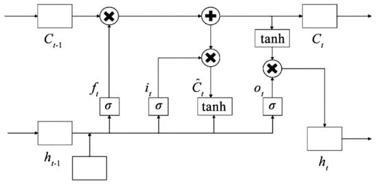
Figure 1.
The structure of LSTM.
The execution process starts at the first layer of the forgetting door, and the calculation formula is as follows:
where is the forgetting gate weight matrix, is the hidden state of the previous moment, is the input of the current time , is the forgetting gate bias parameter, and is the sigmoid function, which is expressed as
with serving as the sigmoid function’s input variable.
The second layer is the input gate, and the corresponding calculation formula is
where is the input gate weight matrix and indicates the input gate bias parameter.
Temporary cell state is calculated as follows:
where is the weight matrix of the layer and is the corresponding bias parameter. Thus, the status update of the storage unit from to can be expressed as
The third layer is the output layer, which is determined via the sigmoid function to partially update the state, and the function constraints the output value within the interval (1,1). The output layer is calculated as follows:
and
where is the output gate weight matrix and is the corresponding bias parameter.
3.4. CNN
A CNN primarily comprises convolutional layers and pooling layers [37]. The convolutional layer performs convolution operations between local regions of the input signal and the convolution kernels within filters, producing nonlinear mappings through the action of an activation function. Each filter can extract different local features from the input signal. The output of a filter corresponds to a frame in the next layer, and the number of frames is referred to as the depth of that layer. The convolutional layer uses wide convolution kernels, and the convolution process is described below:
where and respectively represent the weight matrix and bias term, within the m-th convolution kernel in the l-th layer; represents the n-th region of the l-th layer; and represents the output after convolution of the m-th convolution kernel in the n-th region of the (l + 1)-th layer.
After convolution, an activation function is applied to introduce non-linear characteristics, thereby enhancing the model’s feature representation capabilities. The ReLU (rectified linear unit) activation function is utilized to accelerate the convergence process of the CNN. The corresponding expression is as follows:
where is the output value after activation of .
Pooling effectively reduces the feature space and network parameters after CNN convolution. The most-used pooling layers are average pooling and max pooling. In this paper, the max pooling layer is adopted, which performs max pooling operations on feature information to reduce parameters and decrease data dimensionality. The max pooling operation is as follows:
where represents the value of the t-th neuron in the m-th frame of the l-th layer, m is the width of the pooling area, and represents the value corresponding to the neurons in layer l + 1 after the pooling operation.
3.5. ARIMA
As a statistical forecasting model, the ARMA model exhibits excellent predictive performance for stationary data. However, for non-stationary data, differencing operations are first required. ARIMA [38] models the current time series value as a linear function of past observations.
Let a model be
where represent historical data values and are the measurement errors with the same mean of zero and different constant variances. The auto-regressive moving-average ARIMA (p,d,q) is adopted after D-order difference stabilization, where AR stands for “autoregressive”, I represents the difference calculation, and MA stands for “moving average”. p is the number of autoregressive terms, d represents the difference number, and q is the number of moving-average terms.
3.5.1. AR Model
The AR model predicts future data based on historical data. The formula for a p-th order autoregressive process is defined as follows:
where stands for the value of time t, is a constant term, is the autoregressive order, is the autocorrelation coefficient, and is the error.
3.5.2. MA Model
The MA model accumulates the error terms in the model regression. The formula for a q-order moving-average process is
where stands for the value of time t, is a constant term, is the moving-average coefficient, is the moving-average order, and is the error.
3.5.3. Parameter Determination
- (1)
- Determination of p and q
The process of determining ARIMA model parameters is detailed in the following Table 1.

Table 1.
ARIMA model parameter determination.
- (2)
- Information criteria law
The performance of a model fit is often evaluated using the AIC (Akaike Information Criterion), which is based on the concept of entropy in information theory. The AIC is a measure of the relative quality of statistical models for a given set of data. The formula for the AIC is as follows:
where represents the number of parameters in the fitted model, is the log-likelihood of the model, and n is the number of observations. The value of the AIC is correlated with the values of and . A smaller value of indicates a more parsimonious model structure, while a larger value of signifies a more precise model fit. Ultimately, a smaller AIC value indicates a superior model fit.
4. Methodology
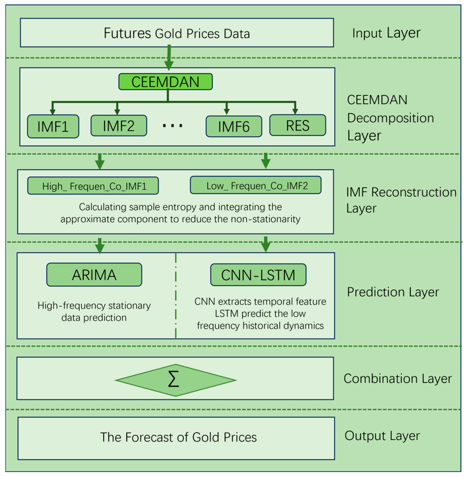
Financial time series data exhibit high-frequency instability, random complexity, and non-linearity. To better fit the real data, our time series prediction algorithm based on the ARIMA-CNN-LSTM hybrid model and CEEMDAN-SE decomposition is as follows:
- Input the original data and use the CEEMDAN algorithm to obtain the decomposed intrinsic mode functions (IMFs).
- Calculate the sample entropy values of each IMF. Components with similar complexities are integrated into Co-IMF components to reduce non-stationarity and non-linearity.
- For the high-frequency stationary Co-IMF components, use the ARIMA model for prediction. For the low-frequency Co-IMF components containing historical trend dynamic information, use the CNN-LSTM model for prediction.
- Overlap the predicted results of each Co-IMF to obtain the final prediction and conduct error analysis.
A flowchart representing this process is shown below (Figure 2):
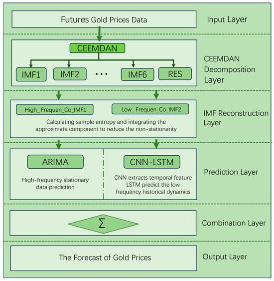
Figure 2.
The flowchart of the hybrid prediction model.
The evaluation metrics for this experiment include the Root Mean Square Error (RMSE), Mean Absolute Error (MAE), and Mean Absolute Percentage Error (MAPE), and their specific formulas are as follows:
where stands for number of observations, is the i-th actual observation, and is the i-th predicted value.
5. Experimental Work
5.1. Experimental Environment
The experiment was carried out using a computer with Windows 10 operating system with an Intel(R)Core (TM) i9-13400F, a NVIDIA GTX4060, and 16.00 GB of RAM. The programming language used for the experiment was Python 3.8.0, and the compiler used was PyCharm 2022 1.0 × 64. Anaconda 22.9.0 was used as the platform for deep learning training, and Keras 2.9.0 and TensorFlow 2.9.1 were used as the deep learning framework.
5.2. Data Collection and Analysis
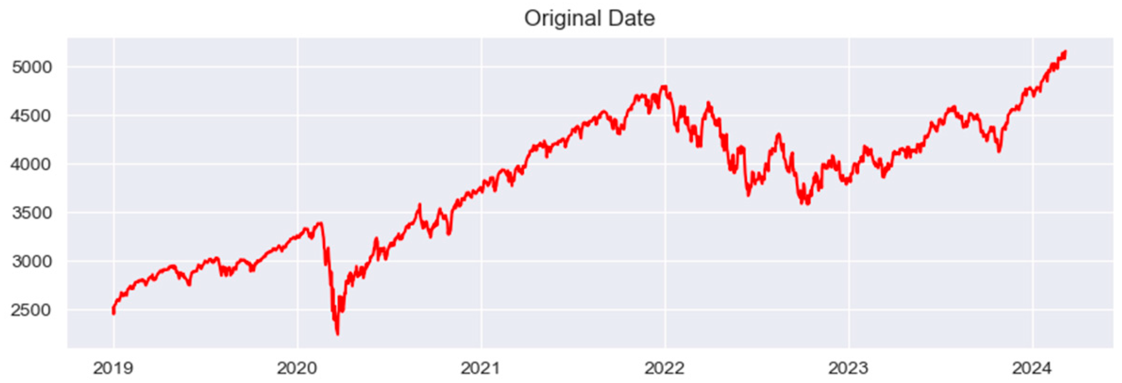
The dataset for this experiment was compiled from the gold futures prices released by the New York COMEX exchange and the gold spot prices published by the World Gold Council. The data on the gold futures price were collected from the following website: https://www.commex.com. The time period covered extends from 1 January 2019 to 18 September 2023, encompassing a total of 1120 data points. And the visualization results of the experimental data are shown below (Figure 3):
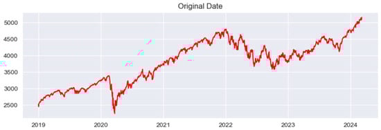
Figure 3.
The original data.
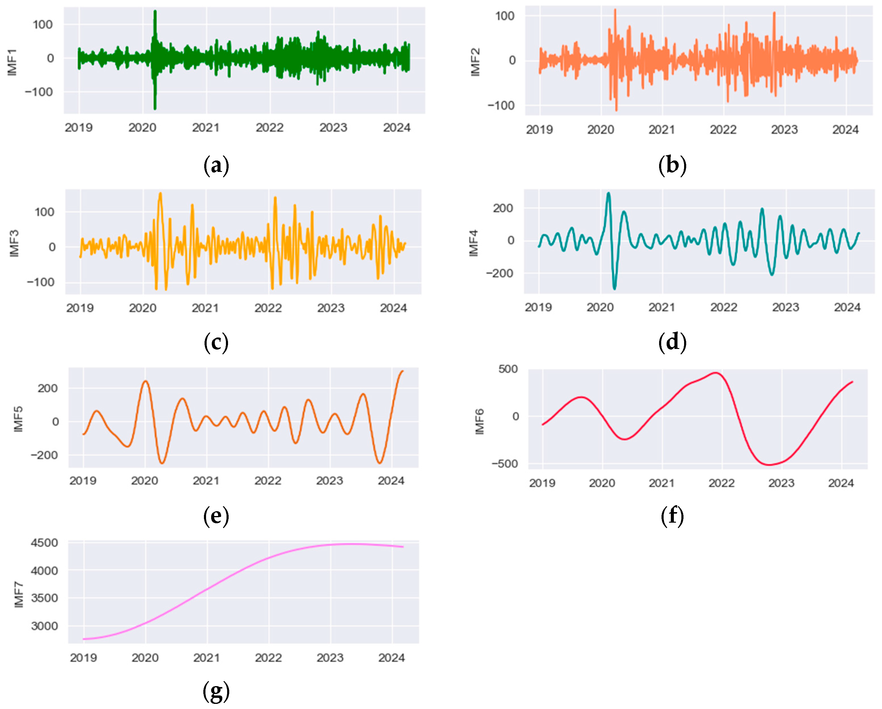
The components of the original data obtained via CEEMDAN decomposition are shown in the figure below (Figure 4):
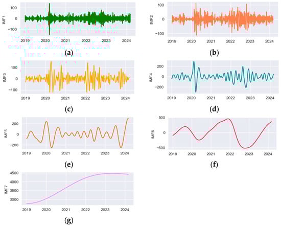
Figure 4.
(a) IMF1. (b) IMF2. (c) IMF3. (d) IMF4. (e) IMF5. (f) IMF6. (g) IMF7.
5.3. Sample Entropy Complexity Calculation for Each IMF
If the LSTM prediction is directly applied to each component, the computational complexity is high, and the prediction accuracy is not optimal. The reason for this is that the LSTM, based on artificial neural network models, can capture historical long-term trends well. However, for high-frequency, random, and complex data components, it does not provide an optimal fit. Therefore, first, the complexity of the time series was described using sample entropy, and for high-frequency data, the statistical model ARIMA was used for prediction. The sample entropy parameters selected were m = 2 and r = 0.2 to calculate the values of each component, as shown in the following table (Table 2):
Table 2.
Sample entropy of each IMF.
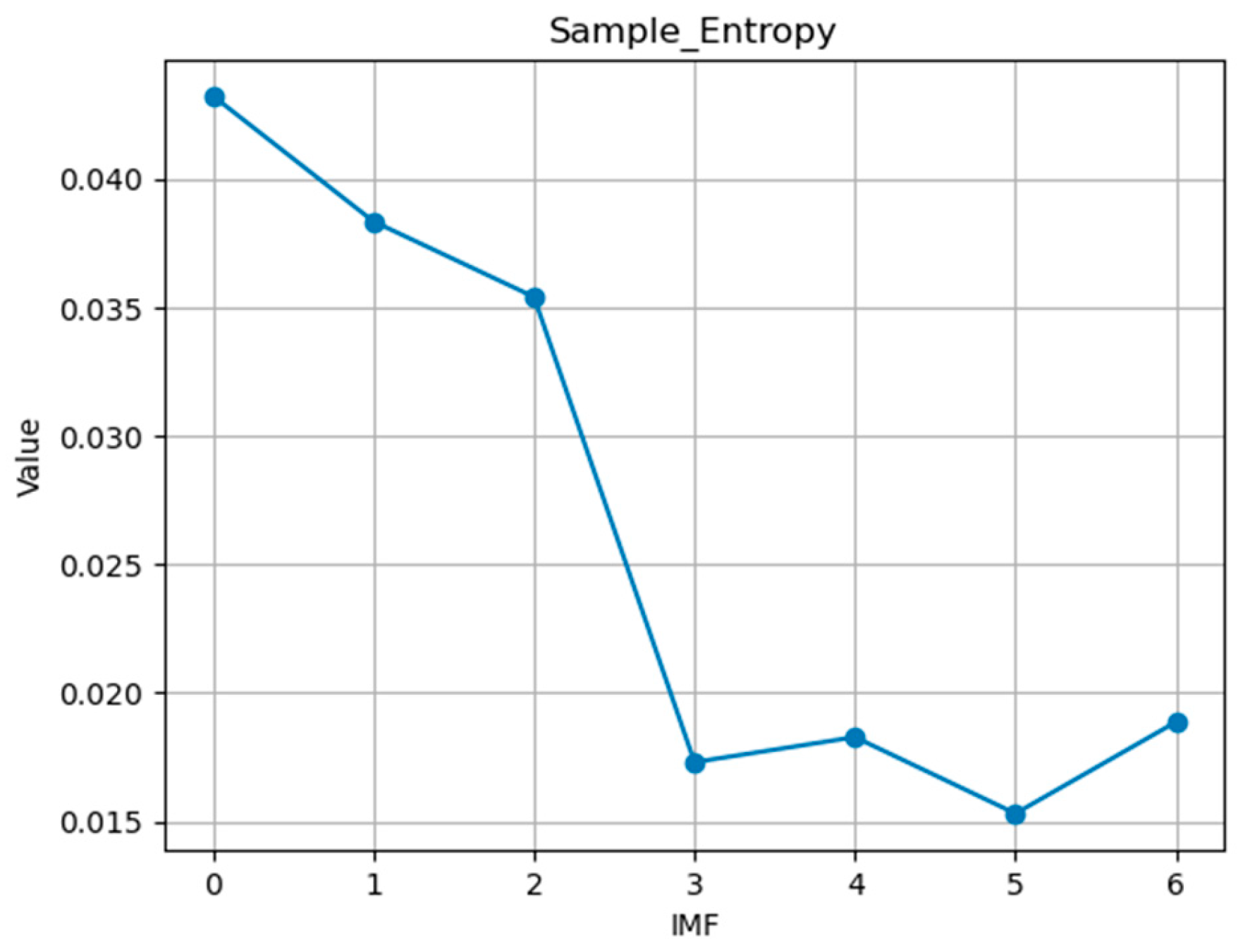
According to the information in the figure, the ranges of sample entropy values for IMF1-IMF3 are similar, with the sample entropy values for the first three components fluctuating between 0.0307 and 0.0328. For the last four components, IMF4-IMF7, the sample entropy values range between 0.0193 and 0.0223. The sample entropy of each component is shown in Figure 5.
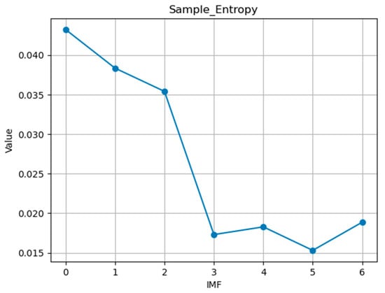
Figure 5.
Sample entropy for each IMF.
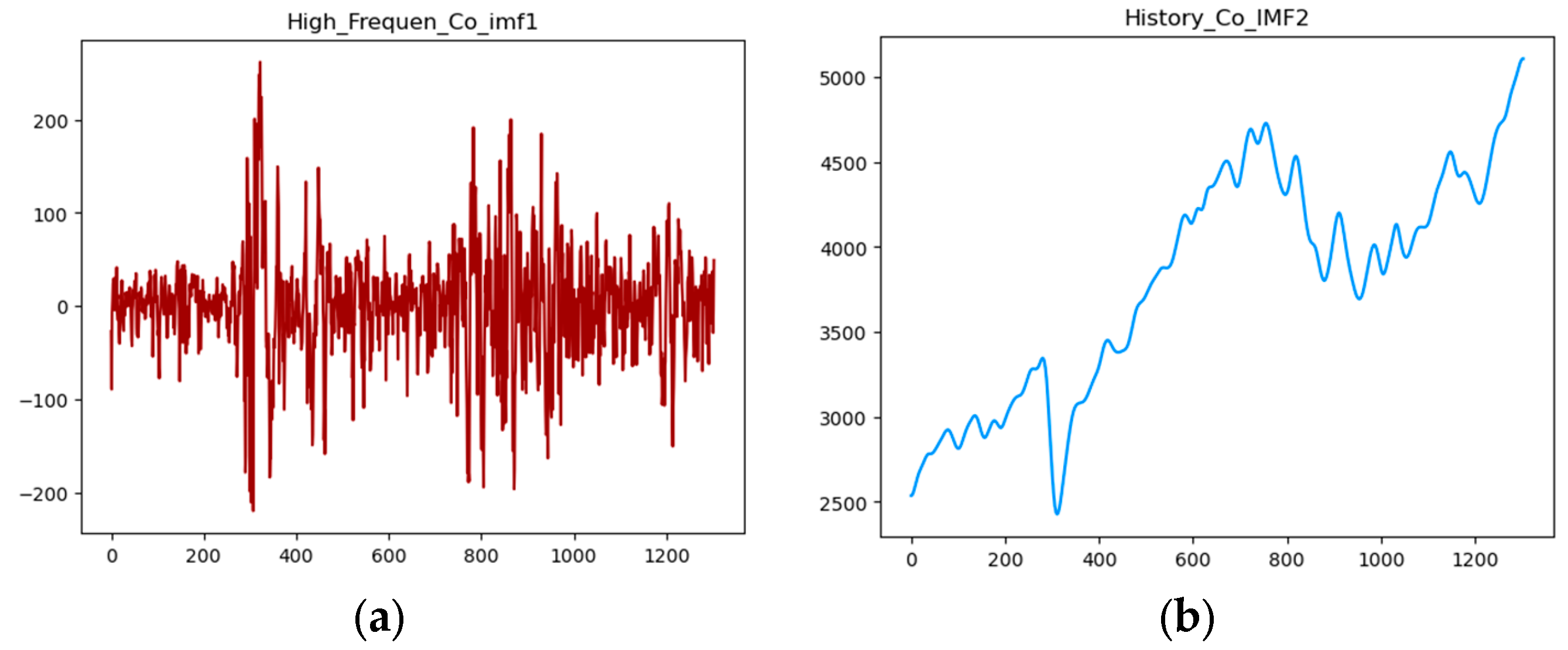
Based on the sample entropy of each IMF, the first three components can be integrated to represent the high-frequency oscillation sequence Co-IMF1, and the last four components can be integrated to represent the sequence Co-IMF2 that includes historical trends. A graph representing this integration is shown below in Figure 6.
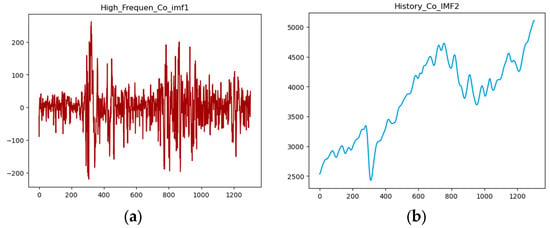
Figure 6.
(a) High_Frequen_Co-IMF1 and (b) History_Co-IMF2.
5.4. Determination of ARIMA for Co-IMF1 and the Prediction Result
- Test the Augmented Dickey–Fuller (ADF) value of the original data and generate Autocorrelation Function (ACF) and Partial Autocorrelation Function (PACF) plots of the original data.
- If the original data are non-stationary, perform differencing operations on the data at time t and t − 1 to achieve stationarity. Then, based on the plots, determine whether further differencing is necessary.
- Determine the order of the model parameters based on the Akaike Information Criterion (AIC) or Bayesian Information Criterion (BIC).
- Establish an ARIMA model using the parameters obtained from step 3 and obtain the results. Diagnose the model by examining the residuals obtained. If the model’s accuracy is low, re-select the model parameters.
In this experiment, the integrated high-frequency Co_IMF1 sequence was used, with the first 1158 data points used as the training set to predict the price curve for the next 30 days, and the last 30 data points served as the validation set. The results of the Augmented Dickey–Fuller (ADF) test for stationarity are as follows:
T-Statistic: −12.130488789892121.
p-value: 1.7405046813662053 × 10⁻²².
In the given results, the test T-statistic is −12.1305, which is a relatively small negative number, suggesting that the time series may be stationary. The p-value is 1.7405 × 10⁻²², which is significantly smaller than the commonly used significance level of 0.05. Therefore, the null hypothesis was rejected, indicating that the time series is stationary and does not contain a unit root. This means that the mean, variance, and autocorrelation structure of the time series do not change over time, satisfying the conditions for stationarity.
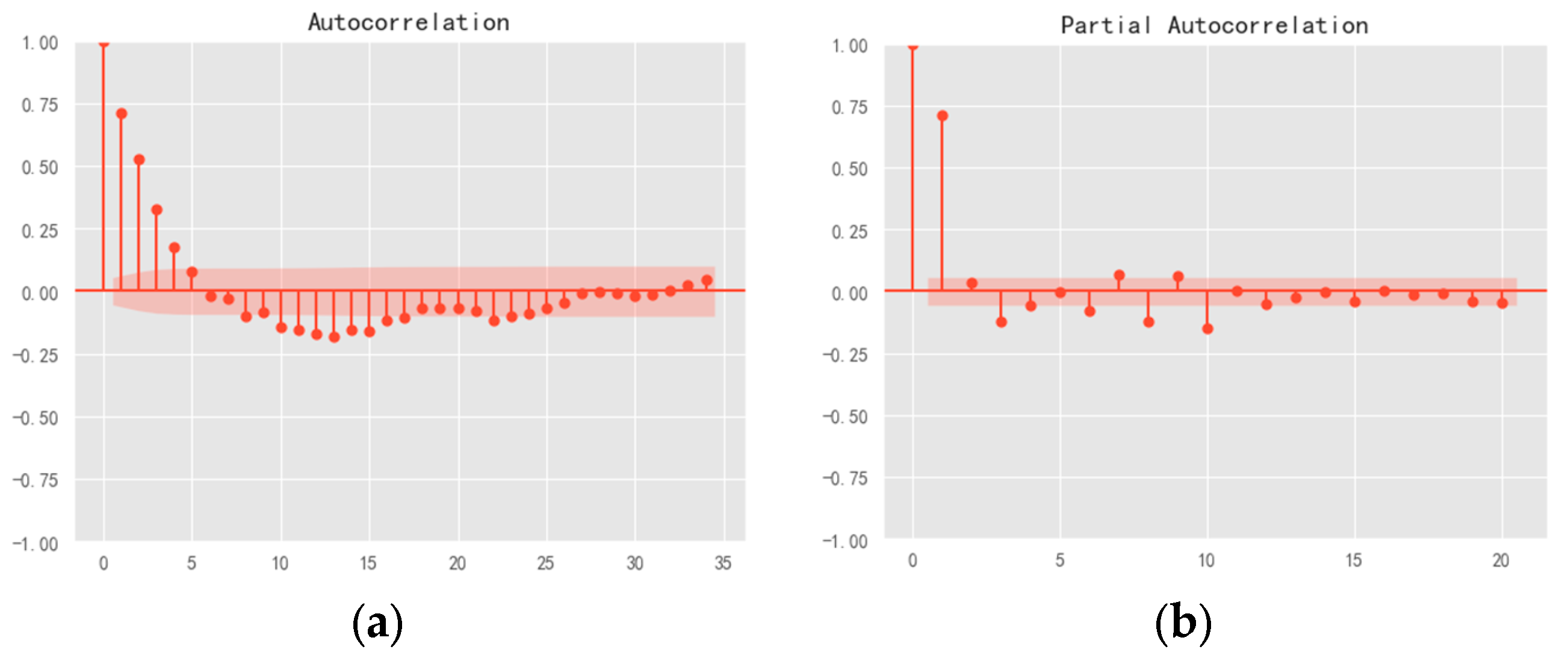
The ACF diagram and PACF diagram are as follows (Figure 7):
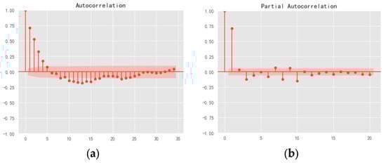
Figure 7.
(a) Autocorrelation and (b) partial autocorrelation.
The Autocorrelation Function (ACF) plot illustrates the correlation between a time series and its lagged values. The Partial Autocorrelation Function (PACF) plot, on the other hand, depicts the partial correlation between the time series and its lagged values. If the ACF cuts off at lag q, it can be concluded that the model is as MA(q). If the PACF cuts off at lag p, it can be determined as AR(p).
Analysis of the ACF and PACF plots reveals that both exhibit oscillatory behavior, indicating good persistence or tailing. The first four lags exhibit values exceeding twice the standard deviation, while subsequent lags do not show a clear excess over twice the standard deviation. Moreover, the transition from significant non-zero values to oscillations near zero occurred relatively quickly. Based on these observations, it was preliminarily determined that the ACF plot is four-order-truncated.
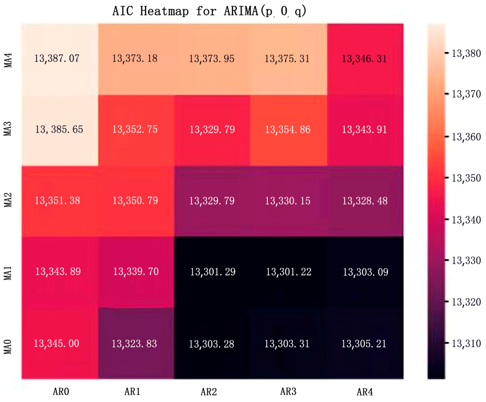
Finally, the parameters of the ARIMA model were determined to be (3, 0, 1) according to the heat map of the Akaike information value, and this heat map is shown below (Figure 8).
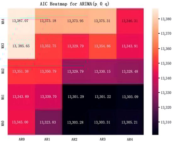
Figure 8.
Heatmap values of the ARIMA model.
Finally, the determined parameters were used for model fitting, employing the DW (Durbin–Watson) statistical test and the Ljung-Box Q statistical test. The DW value determined was 1.9966, which is closer to 2, indicating that there is no significant autocorrelation among the residual series, which means the residual series are independent. The p-value for the Ljung-Box Q test was 0.9813, which is much larger than the commonly used significance level of 0.05. Therefore, the null hypothesis cannot be rejected, suggesting that the residual series is a white noise sequence. These validations indicate that the residual series is non-autocorrelated and random, further confirming the good fit of the model.
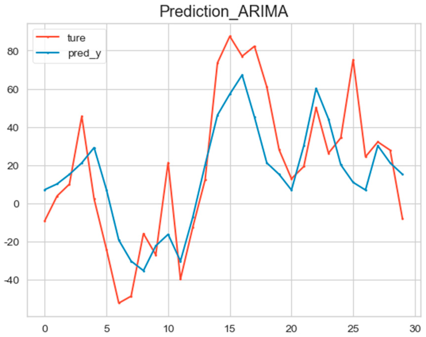
The ARIMA model (3, 0, 1) was used to predict the high-frequency Co-IMF1 data, and the prediction results are shown in the following figure (Figure 9).
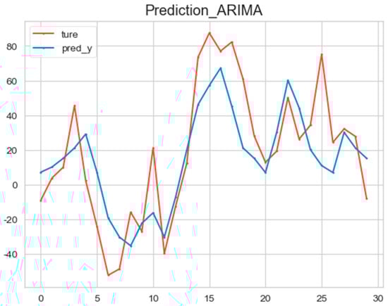
Figure 9.
The prediction result of the ARIMA model.
5.5. CNN−LSTM Prediction Model for Co−IMF2 and the Prediction Result
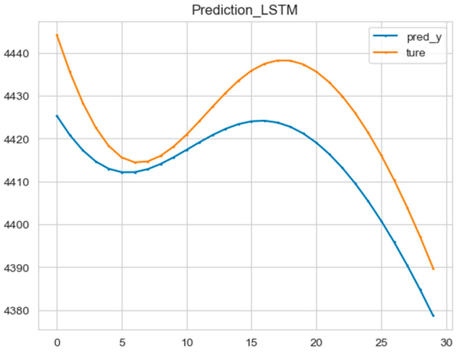
First, the historical dynamic data of Co-IMF2 were normalized using the MinMaxScaler function. Then, the original 1200 data points were divided into a training set and a validation set in a ratio of 8:2. The network structure parameters were defined as follows: the one-dimensional convolutional filter was set to be 32, kernel_size was set to be 2, and the activation was set to be sigmoid. The input dimension of the LSTM was 1, the hidden state dimension was 64, the number of LSTM layers was 5, and the training period was set to 500, with 64 data points per training batch. The Adam optimizer was used, with a learning rate of 0.001. The prediction results are shown in the following figure (Figure 10).
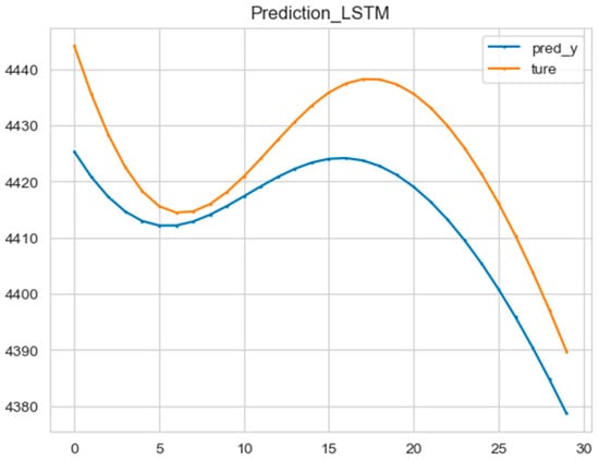
Figure 10.
The prediction result of the CNN-LSTM model.
5.6. Final Result and Error Evaluation
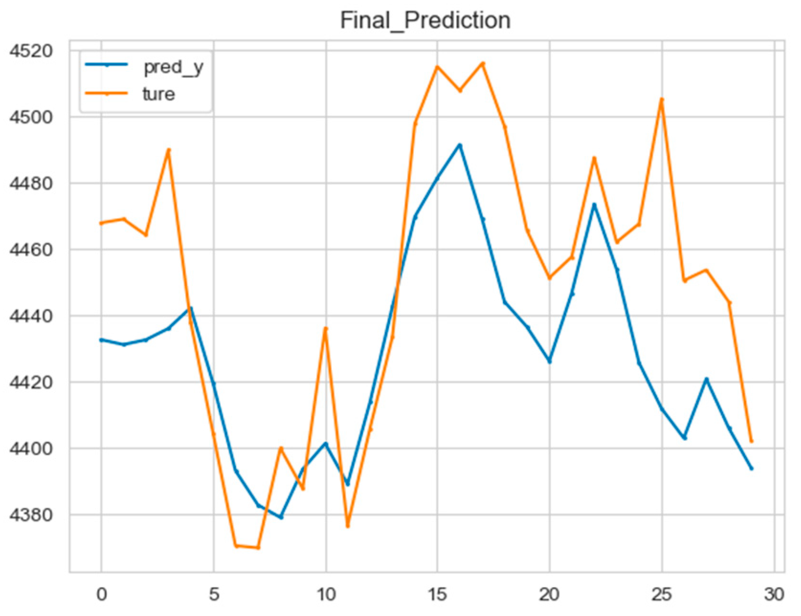
The ARIMA model and CNN-LSTM model were superimposed, and the error between them and the real price curve was calculated, as shown in the figure below (Figure 11):

Figure 11.
The final prediction of the hybrid model.
In this experiment, a comparative analysis of models was conducted, selecting the models LSTM, GRU, and CNN individually, as well as hybrid models. The method of directly predicting the original data without decomposition and reconstruction was compared with the proposed model based on decomposition and reconstruction in this paper. The Root Mean Square Error (RMSE), Mean Absolute Error (MAE), and Mean Absolute Percentage Error (MAPE) were used as evaluation metrics, with the results presented in the following table (Table 3).
Table 3.
The results of the comparative analysis.
Based on the comparative analysis of LSTM and GRU individually, the LSTM, which includes three gates and a cell state, is better at capturing long-term historical trends compared to the simplified GRU structure. This is reflected in the RMSE, MAE, and MAPE, which were reduced by 46.98, 36.86, and 0.82%, respectively, indicating that the LSTM model is more effective for long-term historical predictions. When comparing the convolutional hybrid models CNN-LSTM and CNN-GRU and the individual models, it can be gleaned that the addition of the CNN module resulted in a decrease in the RMSE, MAE, and MAPE errors of 12.14, 13.45, and 0.3% for the LSTM model and a decrease of 12.67, 10.25, and 0.23% for the GRU model. The analysis shows that the CNN performed well in extracting the volatility and frequency characteristics of time series data. Overall, the ARIMA-CNN-LSTM method based on CEEMDAN-SE decomposition and reconstruction proposed in this paper achieves relatively accurate precision in time series prediction.
6. Conclusions
For the task of non-stationary, stochastically complex financial time series prediction, we selected the gold futures prices as the prediction object because they have always played a crucial role in the global economy and finance, and we also proposed a method that combines statistical learning and deep learning to predict the sequences based on the decomposition and reconstruction method using CEEMDAN-SE. This algorithm first decomposes the raw data into a series of IMFs, significantly reducing nonlinearity and non-stationarity, and then calculates the sample entropy values of each IMF. To reduce computational complexity, the sequences with similar entropy values are integrated into the low-frequency and high-frequency components. For the high-frequency components, the ARIMA model was selected, and for the low-frequency components, the CNN-LSTM model was chosen. To enhance the practicality and scalability of the model presented in this paper, future studies could consider expanding the range of experimental prediction targets, such as crude oil prices and international natural gas prices. Another focal point of research in this area is feature selection for the prediction targets, including average daily prices, average opening prices, average closing prices, average highest and lowest prices, daily trading volumes, and economic technical trading indicators. The selection of different features is also of great importance for predicting final prices [39].
The comparison models include the GRU model and the CNN-GRU model with added convolutional blocks. The single LSTM model outperformed the GRU model in terms of RMSE, MAE, and MAPE errors. With added CNN modules, the CNN-LSTM model and the CNN-GRU model have lower RMSE, MAE, and MAPE errors compared to the single models. Additionally, the ARIMA-CNN-LSTM hybrid model proposed in this paper exhibited the best performance in the comparative experiments.
In summary, the following conclusions can be drawn:
- (1)
- The hybrid model that combines statistical learning and deep learning performs better than the individual models.
- (2)
- For low-frequency components, LSTM is more effective than GRU in capturing long-term historical dynamics.
- (3)
- Adding CNN convolutional blocks can better extract the fluctuation characteristics of time series.
Future work can further explore different combinations of statistical and deep learning models, such as by considering seasonal differencing with the SARIMA model and adding attention mechanisms to neural networks. Additionally, various external factors can impact the price of gold, such as the global economic situation, sudden political events, natural disasters, and so on. Considering that this experiment did not include a sentiment analysis module, in future research, we plan to incorporate sentiment analysis of news media texts and use it as an influencing factor to enhance the accuracy of our predictions.
Author Contributions
Conceptualization, Z.D.; methodology, Z.D.; software, Z.D.; validation, Z.D.; writing—original draft, Z.D.; formal analysis, Y.Z.; data curation, Y.Z.; writing—review and editing, Y.Z.; supervision, Y.Z.; project administration, Y.Z.; funding acquisition, Y.Z. All authors have read and agreed to the published version of the manuscript.
Funding
This document is the result of a research project funded by the Natural Science Foundation of China (11861025), the QKZYD of Guizhou [2022]4055, the Natural Science Research Project of the Guizhou Provincial Department of Education (No. QJJ [2023] 011), and Guizhou Provincial QKHPTRC-BQW [2024]015.
Data Availability Statement
The data used in this paper are all from the gold futures prices released by the New York COMEX exchange and the gold spot prices published by the World Gold Council.
Conflicts of Interest
The authors declare no conflicts of interest.
References
- Zhou, F.; Zhang, Q.; Sornette, D.; Jiang, L. Cascading logistic regression onto gradient boosted decision trees for forecasting and trading stock indices. Appl. Soft Comput. 2019, 84, 105747. [Google Scholar] [CrossRef]
- Yu, H.; Chen, R.; Zhang, G. A SVM stock selection model within PCA. Procedia Comput. Sci. 2014, 31, 406–412. [Google Scholar] [CrossRef]
- Alfonso, G.; Ramirez, D.R. Neural Networks in Narrow Stock Markets. Symmetry 2020, 12, 1272. [Google Scholar] [CrossRef]
- Heo, W.; Kim, E.; Kwak, E.J.; Grable, J.E. Identifying Hidden Factors Associated with Household Emergency Fund Holdings: A Machine Learning Application. Mathematics 2024, 12, 182. [Google Scholar] [CrossRef]
- Jeong, G.; Kim, H.Y. Improving financial trading decisions using deep Q-learning: Predicting the number of shares, action strategies, and transfer learning. Expert Syst. Appl. 2019, 117, 125–138. [Google Scholar] [CrossRef]
- Nabipour, M.; Nayyeri, P.; Jabani, H.; Mosavi, A.; Salwana, E. Deep learning for stock market prediction. Entropy 2020, 22, 840. [Google Scholar] [CrossRef]
- Huang, N.E.; Shen, Z.; Long, S.R.; Wu, M.C.; Shih, H.H.; Zheng, Q.; Yen, N.C.; Tung, C.C.; Liu, H.H. The empirical mode decomposition and the Hilbert spectrum for nonlinear and non-stationary time series analysis. Proc. R. Soc. Lond. Ser. A Math. Phys. Eng. Sci. 1998, 454, 903–995. [Google Scholar] [CrossRef]
- Wu, Z.; Huang, N.E. Ensemble empirical mode decomposition: A noise-assisted data analysis method. Adv. Adapt. Data Anal. 2009, 1, 1–41. [Google Scholar] [CrossRef]
- Torres, M.E.; Colominas, M.A.; Schlotthauer, G.; Flandrin, P. A complete ensemble empirical mode decomposition with adaptive noise. In Proceedings of the 2011 IEEE International Conference on Acoustics, Speech and Signal Processing (ICASSP), Prague, Czech Republic, 22–27 May 2011; pp. 4144–4147. [Google Scholar]
- Cao, J.; Wang, J. Stock price forecasting model based on modified convolution neural network and financial time series analysis. Int. J. Commun. Syst. 2019, 32, e3987. [Google Scholar] [CrossRef]
- Pang, X.; Zhou, Y.; Wang, P.; Lin, W.; Chang, V. An innovative neural network approach for stock market prediction. J. Supercomput. 2020, 76, 2098–2118. [Google Scholar] [CrossRef]
- Hochreiter, S.; Schmidhuber, J. Long short-term memory. Neural Comput. 1997, 9, 1735–1780. [Google Scholar] [CrossRef]
- Cao, J.; Li, Z.; Li, J. Financial time series forecasting model based on CEEMDAN and LSTM. Phys. A Stat. Mech. Its Appl. 2019, 519, 127–139. [Google Scholar] [CrossRef]
- Fjellström, C. Long short-term memory neural network for financial time series. In Proceedings of the 2022 IEEE International Conference on Big Data (Big Data), Osaka, Japan, 17–20 December 2022; pp. 3496–3504. [Google Scholar]
- Hoseinzade, E.; Haratizadeh, S. CNNpred: CNN-based stock market prediction using a diverse set of variables. Expert Syst. Appl. 2019, 129, 273–285. [Google Scholar] [CrossRef]
- Shi, Z.; Hu, Y.; Mo, G.; Wu, J. Attention-based CNN-LSTM and XGBoost hybrid model for stock prediction. arXiv 2022, arXiv:2204.02623. [Google Scholar]
- Chen, L.; Chi, Y.; Guan, Y.; Fan, J. A hybrid attention-based EMD-LSTM model for financial time series prediction. In Proceedings of the 2019 2nd International Conference on Artificial Intelligence and Big Data (ICAIBD), Chengdu, China, 25–28 May 2019; pp. 113–118. [Google Scholar]
- Yu, L.; Wang, S.; Lai, K.K. Forecasting crude oil price with an EMD-based neural network ensemble learning paradigm. Energy Econ. 2008, 30, 2623–2635. [Google Scholar] [CrossRef]
- Shu, W.; Gao, Q. Forecasting stock price based on frequency components by EMD and neural networks. IEEE Access 2020, 8, 206388–206395. [Google Scholar] [CrossRef]
- Tang, L.; Wu, Y.; Yu, L. A randomized-algorithm-based decomposition-ensemble learning methodology for energy price forecasting. Energy 2018, 157, 526–538. [Google Scholar] [CrossRef]
- Tang, L.; Lv, H.; Yu, L. An EEMD-based multi-scale fuzzy entropy approach for complexity analysis in clean energy markets. Appl. Soft Comput. 2017, 56, 124–133. [Google Scholar] [CrossRef]
- E, J.; Ye, J.; Jin, H. A novel hybrid model on the prediction of time series and its application for the gold price analysis and forecasting. Phys. A Stat. Mech. Its Appl. 2019, 527, 121454. [Google Scholar] [CrossRef]
- Zhou, S.; Lai, K.K.; Yen, J. A dynamic meta-learning rate-based model for gold market forecasting. Expert Syst. Appl. 2012, 39, 6168–6173. [Google Scholar] [CrossRef]
- Liang, Y.; Lin, Y.; Lu, Q. Forecasting gold price using a novel hybrid model with ICEEMDAN and LSTM-CNN-CBAM. Expert Syst. Appl. 2022, 206, 117847. [Google Scholar] [CrossRef]
- Vidal, A.; Kristjanpoller, W. Gold volatility prediction using a CNN-LSTM approach. Expert Syst. Appl. 2020, 157, 113481. [Google Scholar] [CrossRef]
- Lee, Y.H.; Kim, E. Deep Learning-based Delinquent Taxpayer Prediction: A Scientific Administrative Approach. KSII Trans. Internet Inf. Syst. 2024, 18, 30–45. [Google Scholar]
- Yang, Y.; Yang, Y. Hybrid method for short-term time series forecasting based on EEMD. IEEE Access 2020, 8, 61915–61928. [Google Scholar] [CrossRef]
- He, K.; Ji, L.; Wu, C.W.D.; Tso, K.F.G. Using SARIMA–CNN–LSTM approach to forecast daily tourism demand. J. Hosp. Tour. Manag. 2021, 49, 25–33. [Google Scholar] [CrossRef]
- Chung, W.H.; Gu, Y.H.; Yoo, S. District heater load forecasting based on machine learning and parallel CNN-LSTM attention. Energy 2022, 246, 123350. [Google Scholar] [CrossRef]
- Eapen, J.; Bein, D.; Verma, A. Novel deep learning model with CNN and bi-directional LSTM for improved stock market index prediction. In Proceedings of the 2019 IEEE 9th Annual Computing and Communication Workshop and Conference (CCWC), Las Vegas, NV, USA, 7–9 January 2019; pp. 0264–0270. [Google Scholar]
- Livieris, I.E.; Pintelas, E.; Pintelas, P. A CNN–LSTM model for gold price time-series forecasting. Neural Comput. Appl. 2020, 32, 17351–17360. [Google Scholar] [CrossRef]
- Zhang, R.; Yuan, Z.; Shao, X. A new combined CNN-RNN model for sector stock price analysis. In Proceedings of the 2018 IEEE 42nd Annual Computer Software and Applications Conference (COMPSAC), Tokyo, Japan, 23–27 July 2018; Volume 2, pp. 546–551. [Google Scholar]
- Richman, S.; Moorman, R. Physiological time-series analysis using approximate entropy and sample entropy. Am. J. Physiol.-Heart Circ. Physiol. 2000, 278, H2039–H2049. [Google Scholar] [CrossRef]
- Ma, X.; Tao, Z.; Wang, Y.; Yu, H.; Wang, Y. Long short-term memory neural network for traffic speed prediction using remote microwave sensor data. Transp. Res. Part C Emerg. Technol. 2015, 54, 187–197. [Google Scholar] [CrossRef]
- Graves, A.; Graves, A. Long short-term memory. In Supervised Sequence Labelling with Recurrent Neural Networks; Springer: Berlin/Heidelberg, Germany, 2012; pp. 37–45. [Google Scholar]
- Greff, K.; Srivastava, R.K.; Koutník, J.; Steunebrink, B.R.; Schmidhuber, J. LSTM: A search space odyssey. IEEE Trans. Neural Netw. Learn. Syst. 2016, 28, 2222–2232. [Google Scholar] [CrossRef]
- Lecun, Y.; Bottou, L.; Bengio, Y.; Haffner, P. Gradient-based learning applied to document recognition. Proc. IEEE 1998, 86, 2278–2324. [Google Scholar] [CrossRef]
- Valipour, M.; Banihabib, M.E.; Behbahani, S.M.R. Comparison of the ARMA, ARIMA, and the autoregressive artificial neural network models in forecasting the monthly inflow of Dez dam reservoir. J. Hydrol. 2013, 476, 433–441. [Google Scholar] [CrossRef]
- Ma, Y.; Yang, B.; Su, Y. Technical trading index, return predictability and idiosyncratic volatility. Int. Rev. Econ. Financ. 2020, 69, 879–900. [Google Scholar] [CrossRef]

Disclaimer/Publisher’s Note: The statements, opinions and data contained in all publications are solely those of the individual author(s) and contributor(s) and not of MDPI and/or the editor(s). MDPI and/or the editor(s) disclaim responsibility for any injury to people or property resulting from any ideas, methods, instructions or products referred to in the content. |
© 2024 by the authors. Licensee MDPI, Basel, Switzerland. This article is an open access article distributed under the terms and conditions of the Creative Commons Attribution (CC BY) license (https://creativecommons.org/licenses/by/4.0/).