Abstract
In this study, we examine how the strategies of the players over multiple time scales impact the decision making, resulting payoffs and the costs in non-cooperative strategic games. We propose a dynamic generalized Nash equilibrium problem for non-cooperative strategic games which evolve in multidimensions. We also define an equivalent dynamic quasi-variational inequality problem. The existence of equilibria is established, and a spot electricity market problem is reformulated in terms of the proposed dynamic generalized Nash equilibrium problem. Employing the theory of projected dynamical systems, we illustrate our approach by applying it to a 39-bus network case, which is based on the New England system. Moreover, we illustrate a comparative study between multiple time scales and a single time scale by a simple numerical experiment.
Keywords:
game theory; dynamic generalized Nash equilibrium problem; dynamic quasi-variational inequality problem; spot electricity market problem; projected dynamical system MSC:
49J40; 49J50; 90C33
1. Introduction
In order to simplify our presentation and emphasize the novelty of our work, we divide the introduction into two subsections. We start with the background and the relationship to previous works, and then present our own contribution.
1.1. Background and Relationship to Previous Works
A game is a tool for modeling any situation in which players interact and take decision to attain a certain goal. In game theory, there are two different approaches. One is the cooperative game approach started by von Neumann and Morgenstern [1], and the other is the non-cooperative game approach initiated by Nash [2,3]. In the non-cooperative game approach, the players are supposed to choose their actions individually, and selfishly seek their own goals and maximize their own profits. However, this does not mean that players are essentially antagonistic to other players. In fact, they are just not interested in the welfare of other players. In contrast, the cooperative game approach involves the players’ alliances and their willingness to share their benefits obtained from the cooperation. The difference between these two approaches can be concisely formulated as follows: a non-cooperative game describes the various available options of actions for players, while a cooperative game sets out the consequences when the players join each other in different combinations. In continuation of the study of these strategic games, the study of equilibrium problems was initiated by Cournot [4], who considered an oligopolistic economy. However, it was Nash [5,6] who introduced this concept formally. Subsequently, Arrow and Debreu [7] extended it to the generalized Nash equilibrium problem. For getting an overview of generalized Nash equilibrium problems, we refer the interested readers to the survey papers [8,9] and references therein. The generalized Nash equilibrium problem (GNEP) is very useful in mathematical modelings of various real world problems. We can find some of its recent applications in [10,11,12,13], to name but a few. In addition, time-dependent generalized Nash equilibrium problems are also investigated in [14,15]. Generalized Nash equilibrium problems are connected to quasi-variational inequality problems, a fact which was first observed by Bensoussan [16]. Thereafter, Harker [17] investigated these problems in Euclidean spaces. Quasi-variational inequality problems have been proven to be an efficient tool for studying the GNEP; see, for example, Aussel et al. [18]. Recently, Beuno and Cotrina [19] have shown the existence of projected solutions to the GNEP by using a generalization of Berge’s maximum theorem and Himmelberg’s fixed point theorem; see also [20] and references therein. We would also like to mention the very recent interesting relevant articles [21,22], which deal with the GNEP, its reformulation in terms of variational inequality problems, and its applications to the COVID-19 pandemic.
Several patterns of electricity market networks have been structured and studied in the literature. The main concern of this work is the electricity market centralized by an independent system operator (ISO) and the supply chain network perspective. Indeed, the role of the ISO is crucial in spot electricity markets, where the electrical energy is traded for immediate physical delivery, and the ISO schedules the dispatch quantities, prices, and the transmission of electricity. This kind of electricity structure is running successfully in the electric power industry of the United States, United Kingdom, and the Nordic countries. Hu and Ralph [23] studied a bilevel non-cooperative game-theoretic model for the ISO centralized spot electricity market by utilizing the mathematical model of equilibrium programs with equilibrium constraints (EPECs). Later, Aussel et al. [24] studied this bilevel optimization structure of electricity markets involving the influence of transmission losses. For more studies of the spot electricity market operated by an ISO, we refer interested readers to [14,25,26,27] and references therein. On the other hand, an electric power supply chain network model works with the decision-makers which operate in a decentralized manner. In particular, the mechanism of a supply chain network involves power generators, power suppliers (including power marketers, traders, and brokers), transmission service providers, and consumers (demand markets, or end users). Nagurney and Matsypura [28] studied this structure in detail, where the ISO controls the function of transmission service providers so that the prices of the transmission services are reasonable and not discriminatory. However, the price of transmission services is not constant, since it depends on the amount of electric power transmitted, the distance, and so on. Projected differential inclusions and pertinent existence results were first introduced by Henry [29]. Moreover, the book of Nagurney and Zhang [30] provides a study of projected dynamical systems, which not only permit to incorporate constraints, but are also related to the variational inequality problem. Indeed, the stationary points of the ordinary differential equation involved in the projected dynamical system coincide with the solutions to the associated variational inequality problem. Consequently, any equilibrium problem that can be reformulated as a finite-dimensional variational inequality problem can now also be studied as a projected dynamical system. These authors also developed iterative algorithms for computing stationary points of projected dynamical systems and used them to solve oligopolistic market, spatial price, and elastic and fixed demand traffic equilibrium problems. Later, Nagurney et al. [31] used this to study dynamic electric power supply chains as well. For more relevant works, see [32,33,34,35,36].
In parallel, the concept of a multidimensional optimization problem was also being studied. It originated in the calculus of variations in the context of functions of several independent variables. The study of this concept was initiated by Ekeland and Temam [37] in the 1970s. Such problems are also known as multidimensional control problems. Subsequently, the study of the notion of multidimensional optimization problems continued gradually. For example, Guseĭnov [38] investigated an extension of the multidimensional optimization problem, and Fonseca and Marcellini [39] studied the lower semicontinuity and relaxation of the multiple integrals which appear in multidimensional optimization problems. For more relevant studies, we refer the interested readers to [40,41,42,43,44]. In recent decades, Udrişte and Ţevy [45] have introduced the basic optimization problems involving path-independent curvilinear integrals and multiple integrals. They named them multi-time (multiple parameters of evolution) optimal control problems. These problems have evolved from the above-mentioned multidimensional optimization problems. However, the techniques developed and the results established by the research group of Udrişte [46,47,48] are different from those in the aforementioned papers regarding multidimensional optimization problems. It turns out that several science and engineering problems can be converted into optimization problems that are defined as m-flow type PDEs (multi-time evolution systems), where the associated cost functionals are expressed as path-independent curvilinear integrals or multiple integrals. Such cost functionals originated in physics and are known as mechanical work type integrals. For some recent relevant works, we refer the interested reader to [49,50] and references therein.
1.2. Our Contribution
Here, we explain in detail the novelty of our contributions.
- We introduce a dynamic generalized Nash equilibrium problem (DGNEP) in the terms of a path-independent curvilinear integral, which is a functional, and a dynamic quasi-variational inequality problem (DQVIP) over multiple time scales, which we call multiple parameters of evolution. First, we establish an equivalent relationship between the DGNEP and the DQVIP by using the classic tools of convex analysis. However, in this work, we exploit the form of the functionals, given in the terms of path-independent curvilinear integrals, by using the convexity of the considered functional. Furthermore, we also prove the existence of solutions to the DGNEP by exploiting its equivalence with the DQVIP, and by using the techniques of proving existence results for generalized vector quasi-variational inequality and quasi-equilibrium problems, studied in [51,52]. We note that papers [51,52] deal with functions of a finite number of independent variables, but our work deals with functions of a number of independent functions, i.e., functionals, and there is no such ‘universal’ space; indeed, problems are defined in a function space. Moreover, if all the functions are independent of the multiple parameters of evolutions t, then our introduced problems and established results can be converted into the problems and results of the static case, which were studied in [8,9,17,18,19,20,21,22,51,52,53]. In essence, our results can be seen as dynamic generalizations of the corresponding (static) derived results of the aforementioned papers. This outcome promotes a new approach aimed at relationships between mathematical programming and the classical calculus of variations. We recall that Hanson [54], who was the first to observe such kind of relationships, emphasized that some of the duality theorems of mathematical programming have analogues in the variational calculus.
- Our intention is to open a window to understanding and exploring the performance of the decision making models of non-cooperative strategic games with respect to multiple time scales, where we can investigate how the strategy of players over multiple time scales impact the decision making, resulting payoffs, and costs in this kind of games. We emphasize that neither theoretical results, nor experimental results related to generalized Nash equilibrium problems and concerning their applications to electricity market problems, have been investigated so far in the setting of multiple time scales (multiple parameters of evolution). In our recent study [55], we managed to formulate a multi-time generalized Nash equilibrium problem involving multiple integrals, and investigated its theoretical and experimental applications to solving traffic network problems, the aim of which is to minimize the traffic cost of each route, and to solving a river basin pollution problem.
- Motivated by the works of [14,23,24], we formulate a dynamic spot electricity market, which is managed by an ISO in the terms of our DGNEP.
- Following the works of [29,30,31,32,33,34,35,36], we formulate a projected dynamical system (PDS) which pertains to a set-valued map and establish an equivalence relationship between the solutions to the DGNEP and the critical points of the PDS.
- Using the developed PDS theory and synthesizing the data of a 39-bus network case of the New England system taken from the technical report [56], and articles [23,57], we perform several numerical experiments for the dynamic spot electricity market which we formulated.
- We also present a comparative numerical experiment for checking the evolution of resulting payoffs in multiple time scales in comparison to a single time scale. We find that the maximum profit value of each generator in the case of multiple time scales is higher than the corresponding value in the single time scale case.
- Our results also demonstrate how the three theories, (1) ISO-operated spot electricity markets, (2) projected dynamical system theory, and (3) multidimensional optimization problems, which have almost been developed in parallel, can be connected in the single frame of ‘Nash equilibrium problems’ in order to enhance the modeling and analysis of problems that arise in the disciplines of engineering, operations research and management, and economics. More precisely, we use the multidimensional optimization formulations, studied by the research group of Udrişte [46,47,48], to study the GNEP and its application to the ISO centralized dynamic spot electricity market, influenced by [14,23,24] and references therein, by using the techniques of projected dynamical system theory developed by Nagureny’s research group [30,31,32,33,34,35,36]. We would like to mention here that projected dynamical system theory [30,31,32,33,34,35,36] has also been used to study the electricity market from the perspective of supply chain networks.
- Today’s decisions can affect the long-run future. For example, companies like Nike, Disney, Walmart, MacDonald’s, Nestlé, Johnson & Johnson, and many more have realized that their actions in purchasing and supply chain management strongly affect their reputation and long-term success. They have suffered damage to their reputations and sales as a result of public awareness campaigns, external pressure from activists, and internal pressure from investors demanding that companies acknowledge responsibility for labor rights abuses in factories that make their products [58]. The same phenomena also occur in the setting of decision making problems in other industrial areas such as electricity markets and oligopoly markets, and we could go on. Aussel et al. [14], and Cotrina and Zúñiga [15] studied the decision making problem via the GNEP in single time settings, but the above-mentioned long-run effects are not considered by them. The mathematical framework of a decision making problem over multiple time scales makes us capable of capturing the long-term effects, and observing how the decision making, resulting payoffs, and costs evolve in a decision making game when players of such a game make their strategies over multiple time scales. These facts motivated us to study the GNEP in multiple time settings and to examine its application to solving spot electricity market network problems. Multi-period decision making problems with applications in supply chain networks are studied in [59,60] and in the references therein, but our approach and results are completely different from theirs.
The outline of our paper is as follows: preliminaries and formulations of the problem are presented in Section 2. The equivalence of the dynamic generalized Nash equilibrium problem with the quasi-variational inequality problem is established in Section 3. In Section 4, the existence of equilibria is obtained. The formulation of the dynamic spot electricity market model is given in Section 5. The development of a theory of projected dynamical systems is given in Section 6. Numerical experiments with a test case are presented in Section 7. A comparative numerical experiment between multiple time scales and a single time scale is provided in Section 8. Finally, Section 9 concludes our work.
2. Preliminaries and Problem Formulations
We begin our analysis by introducing the following important notations and mathematical tools; for better and deeper insights, we refer the readers to [61].
- (i)
- The abbreviation “a.e.” stands for “almost everywhere”, and represents the set of non-negative vectors in ;
- (ii)
- The non-cooperative strategic game comprises N players;
- (iii)
- in is the planning horizon of players. It is an m-dimensional hypercube with the fixed opposite diagonal points and in , which with the product order relation can be written as ;
- (iv)
- is a piecewise smooth curve joining the opposite diagonal points and in ;
- (v)
- The point is the multiple parameters of evolution, which we call time periods, where is the given time, is another given time, and so on. It follows that the evolution is m-dimensional, which leads us to say that the evolution is multidimensional;
- (vi)
- The dynamic behavior of the non-cooperative strategic game is described by the strategy vector of all the players. In fact, at a given point ;
- (vii)
- is the strategy vector of the player w, i.e., at a given point ;
- (viii)
- is the strategy vector of all the players except player w, i.e., at a given point ;
- (ix)
- ;
- (x)
- To emphasize the strategy vector of the player w, we write the strategy vector x of all the players as . This is just another way of writing the vector ;
- (xi)
- We recall that ;
- (xii)
- is a nonempty, closed, and convex subset;
- (xiii)
- is the nonempty, closed and convex feasible set of the player w for any given strategy vector of the rival players;
- (xiv)
- We say that the strategy vector x of all the players is feasible if for all and for all , we have ;
- (xv)
- We use the following notation, which we need in Section 6, to denote the value of the functional represented by p at the point q:for all , where represents the Euclidean inner product;
- (xvi)
- Each player w has an objective function, which is known as the cost/loss function and which depends on both the player’s own decision variable and on the rival players’ decision variables . We interpret the total cost/loss function that the player w incurs when the rival players have chosen the strategy , , in terms of the path-independent curvilinear integralwhere is the differential element of the multiple parameters of evolution , is a real-valued continuously differentiable function for every and the running cost/loss of the player w, and we use summation over the repeated indices , i.e.,We also assume that the condition , where and are the total derivative operators, is satisfied.
We now provide the following example in order to illustrate and clarify the above discussion.
Example 1.
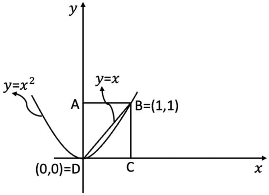
We compute a path-independent curvilinear integral for two-time parameters, i.e., for and . We let be a square with the fixed opposite diagonal points and , i.e., ; see Figure 1. Let the value of the strategy vector at the point be , and . Now, we consider the following two paths of integration, i.e., , just to illustrate the definition of a path-independent curvilinear integral.

Figure 1.
The square ABCD = with the diagonal points and , and the line connecting these points is BD = .
- is the line segment from to ;
- is a parabola from to .
Case 1.
For , on the diagonal connecting the points , , we have . Thus, the value of the integral is
Case 2.
Again, for , we consider the parabola connecting the points , . Thus, the value of the integral is
Evidently, the condition for and is satisfied, and this explains in a simple calculus language that the given vector field is conservative, and the line integral is path-independent.
Remark 1.
From the above example, we deduce the following two evident facts:
- I
- We need to use the condition for and for numerical experiments;
- II
- We can integrate the integrals over and, using a simple calculus rule, we see that the value of the integral is
Next, we formulate the dynamic generalized Nash equilibrium problem as follows:
(DGNEP) find a feasible strategy such that, for all , we have and
Special cases:
- (1)
- If the multiple parameters of evolution are reduced to the single time scale, i.e., and , then and are simply the closed real interval in (the set of non-negative real numbers). We may then write , where T denotes an arbitrary time. Now, the DGNEP reduces to the time-dependent generalized Nash equilibrium problem, which is studied by Aussel et al. in [14].
- (2)
- If all the functions are independent of the multiple parameters of evolution t, then the DGNEP reduces to the generalized Nash equilibrium problem, which is investigated, for example, in [8,9,17,18,19,20,21,22,53].For the formulation of the dynamic quasi-variational inequality problem, we first consider a nonempty, closed and convex subset K of , and define a set-valued map by
We also define a functional by , where is a real-valued continuously differentiable function, , and for and . Moreover, we denote by the partial derivative of the function with respect to the argument x at the strategy vector . The dynamic quasi-variational inequality problem is now formulated as follows.
(DQVIP) to find a vector , such that and
Keeping in mind the definitions of generalized convexities formulated in [62,63], we present the following definition of convexity for the aforementioned functional .
Definition 1.
The functional is said to be convex on the set K if for all , the following inequality holds:
Next, we recall two definitions and a theorem (compare with [51,52]), which are used in the proofs of our results.
Definition 2.
A subset D of K is said to be compactly open (respectively, compactly closed) in K if for any nonempty compact subset L of K, is open (respectively, closed) in L.
Remark 2.
- (a)
- It is evident from the above definition that every open (respectively, closed) set is compactly open (respectively, compactly closed).
- (b)
- The union or intersection of a finite number of compactly open (respectively, compactly closed) sets is compactly open (respectively, compactly closed).
- (c)
- If and are compactly open (respectively, compactly closed) in and , respectively, then is compactly open (respectively, compactly closed) in .
Definition 3.
A family of maps , , is called hemicontinuous if, for all and , the mapping with is continuous, where is the component of v.
Theorem 1
([51]). Assume that are set-valued maps, and the following hypotheses are satisfied:
- ;
- ;
- is convex;
- is compactly open;
- There exists a nonempty, closed and compact subset D of K and such that .
Then, there exists such that .
3. The Dynamic Generalized Nash Equilibrium Problem as a Quasi-Variational Inequality Problem
Our aim in this section is to present an equivalent form of the dynamic generalized Nash equilibrium problem in the terms of a dynamic quasi-variational inequality problem. This equivalent formulation will be beneficial for proving more results later. From now onwards, stands for the partial derivative of the function of a player w for with respect to the argument at the strategy vector .
Theorem 2.
Let for any , and for each and each , assume that the cost functional is convex on K in the argument . Then, is a dynamic generalized Nash equilibrium if and only if it is a solution to the DQVIP.
Proof.
Assume that is a solution to the DQVIP. In order to prove our assertion, we shall first prove that, for , and for each , satisfies the following inequality:
To this end, suppose to the contrary that there exists a and a strategy vector together with a piecewise smooth curve of positive measure, such that, for , the following inequality holds:
Now, we take a strategy vector , defined by
Then, . Thus, we have
By combining inequalities (2) and (3), we obtain
which yields a contradiction with the fact that solves the DQVIP. Consequently, inequality (1) is validated. Furthermore, for each , the convexity of the cost functional on the set K in the argument yields that
Therefore, is the dynamic generalized Nash equilibrium.
Conversely, we suppose that is a dynamic generalized Nash equilibrium, which yields inequality (5). Since is a convex set, for all , inequality (5) can be rewritten as
Dividing the above inequality by , taking the limit as , and using Taylor’s series, we obtain
By the hypothesis, , and so we have, for any ,
Since we already have , it follows that y is a solution to the DQVIP.
□
4. Existence of Equilibria
In this section, we establish the existence of dynamic generalized Nash equilibria. The equivalence of the dynamic generalized Nash equilibrium problem with the dynamic quasi-variational inequality problem allows us to take advantage of the techniques of [51,52]. Throughout this section, we consider the strategy vectors of each player w, and the strategy vectors of rival players excluding the player w, and the subset is given as and , where is a family of nonempty, closed and convex subsets with each . Now, the entire strategy vector can be written as . Furthermore, for all , the strategy set of each player w, is a subset of , and for all , . Using the above mathematical framework, we easily find the following fact:
We assume that, for each , the set is compactly open, and for all , the set is compactly open in . Therefore, Remark 2 (b) and (c) yield that is compactly open for all . Moreover, we also assume that the set is compactly closed.
Theorem 3.
Let be an arbitrary strategy vector, , and for each and a given , let the cost functional be convex on K in the argument . Assume that there exists a nonempty, closed and compact set and , such that
Then, the DQVIP has a solution.
Proof.
In order to prove this result, we first define two set-valued maps as follows: for each , let
and
The convexity of the cost function of each player w on the set K in the arguments of implies that, for all in K, the following inequality holds:
Interchanging the variables and in inequality (7), we are led to the following inequality:
It is evident that the point images of the set-valued maps and are convex for all , a fact which implies the convexity of the point images of the set-valued map for all . Moreover, for all . Now, for all points , we have
Furthermore, for each , the complement of in K can be written as
which is closed in K. Consequently, is open in K. Remark 2 (a) implies that is compactly open for all . We also see that, for all , and are compactly open. Hence, using the above formulation of , we find that it is also compactly open for all . Now, suppose that, for all , . On the other hand, we already know that the point images of the set-valued map are nonempty and convex for all . It follows that for all . Our hypothesis yields that there exist a nonempty and compact set and a point , such that . Thus, all the hypotheses of Theorem 1 are satisfied. This implies that there exists a point such that . The definitions of the set B and the set-valued map T imply that . Therefore, and . Consequently, . It follows that
which is impossible. Thus, we have reached a contradiction, and so there does exist a point such that . That is, and
By using the convexity of both sets and , we can, for all , rewrite the above inequality as
Since is hemicontinuous, by taking the limit as in the above inequality, we obtain
Using the hypothesis, we can rewrite the above inequality as
In other words, is a solution to the DQVIP, as asserted. □
5. The Dynamic Spot Electricity Market Problem
In this section, we first give some arguments in favor of the key element of this work, i.e., “multiple parameters of evolution ”. Moreover, we also explain what we model with the help of these multiple parameters of evolution, and why this is interesting and applicable. Furthermore, we demonstrate how the introduced concept of the DGNEP is associable with electricity markets.
In order to describe multiple parameters of evolution in a real world situation, we take a simple electricity spot market scenario, which is centralized by an independent system operator (ISO), the only agents in the market are generators/producers and the demands on each generator are inelastic and known. The non-cooperative strategic game model in this section is profit-seeking by each agent, which entails a bilevel optimization problem. This works as follows: each agent bids the cost of production of electricity to the ISO. This is a function of the multiple parameters of evolution . The ISO determines the best possible quantities of electricity at a given parameter by minimizing the social cost and then sends them off to each agent. Our model determines how much each agent should bid as the cost of production of electricity at a given to the ISO, so that the agents could maximize their own profit. The ISO’s social cost minimization problem is the lower-level program, while the profit maximization problem of the agents is a bilevel optimization. For a deeper understanding of this kind of a model, we refer the readers to [14,23], where Hu and Ralph [23] studied this electricity market model in the static case and Aussel et al. [14] studied it in the dynamic case only for a single time-parameter of evolution . We are also studying it in the dynamic case, but for multiple parameters of evolution .
Now, our arguments are as follows in order to gain the maximum profit for the long run future, the bidding strategy of producing electricity in the present time can depend on several factors such as the uncertain situation of the markets, the capacities of the generators, and many more, which here we could call the multiple parameters of evolution. This is why the multiple parameters of evolution could also be motivated differently. For instance, could be the time period of generation/delivery of electricity, could be the capacity of the generator to produce electricity, could be the uncertainty of the future. For example, in wind farms, the electricity generation situation depends on the uncertainty of the availability of natural wind. However, in our work, we take all of the parameters as time periods, and the strategy vectors, which are the bidding parameters of producing electricity, depend on or, simply said, are a function of . The motivation behind taking multiple parameters of evolution is to check the long-run effects of our current decisions. For example, if agents have to gain maximum profit by the end of the year 2050, for that, they have to make decisions for bidding the price of producing electricity here-and-now (say, in 2024). In this case, agents probably make decisions according to the first year, second year, third year, and so on up to the year 2050. Mathematically, we can consider the multiple parameters . At this point, one can ask “why not to take the multiple parameters of evolution as a single time parameter, i.e., , and study the model according to Aussel et al. [14]?”. We would like to emphasize here that we do not oppose this single time parameter approach, but as a matter of fact, the here-and-now decision cannot be taken directly for the long term future in one shot, because we also have to deal with other factors and uncertain situations of the future. This kind of situation can also be modeled using stochastic optimization by considering several possible scenarios of the future, but we do not use stochastic optimization in the present work. It is beneficial to take the decision according to small time periods by dividing long future time periods into several small periods of times, i.e., according to the multiple parameters of evolution, so that we can capture all the factors, which probably change every year and affect our current decisions in order to gain the maximum profit for the long run. This is what we try to illustrate in Section 8 by providing a simple numerical example, which shows that the maximum profit in the terms of multiple parameters of evolution is greater than the one obtained in the single time parameter case. However, in the present work, because we did not apply any real world data to check this fact, we plan to do this in our future work. We just try to justify the use of multiple parameters of evolution in the context of Nash equilibrium problems by providing some simple numerical evidence and by exploiting the structure of multidimensional optimization problems in the terms of curvilinear path-independent integrals, which were studied in [46,47,48,61] and references therein.
In order to define the model in terms of the DGNEP, we assume that the dynamic spot electricity market has N nodes and evolves over the multiple parameters of evolution , defined as in Section 2. We also assume that each node consists of only one generator/producer . Let denote the set of nonnegative real numbers, be the demand function, be the quantity of generated electricity (production function) by the generator w, be the quantity of generated electricity by all the generators except the generator w, and be the true cost to generate units of electricity by the generator w, where are the true parameter values. Next, we consider the dynamic spot electricity market problem in the terms of a bilevel optimization problem, where the following ISO problem is known as the lower-level program of the bilevel program.
5.1. The ISO Problem
Each generator bids an electricity generating cost to the ISO. Thus, the generator provides the bid function (bid generation cost) to the ISO, where the parameters are the bid parameters. Then, the ISO computes the production function for each generator w. Keeping in mind a fact pointed out by Aussel et al. [24], namely that if the distance between the generators is quite small, then it is reasonable to assume that there are no thermal losses, we assume that the thermal losses are negligible, and thus the total demand function on the whole network is given by . Now, clearly, the bid vectors and , given by the generators, are known to the ISO. Thus, the ISO computes a production vector in order to minimize the total generation cost bidden by all the generators. In other words, the ISO has to solve the following optimization problem:
The solution set of the optimization problem (10) is denoted by . In order to continue our study, we define the following set for a given :
5.2. The Generator Problem
Evidently, generators are dependent on each other, at least because of the finiteness of the demand, and they want to maximize their profit. Every generator w bids an electricity generating cost to the ISO, and then each generator w receives the best quantity of electricity from the ISO. Moreover, the market price of the generating electricity for the generator w is the marginal price, which is the derivative of the bid generation cost of the generator w, i.e., . Thus, the generator w receives the revenue . Therefore, the profit of the generator w is defined by . We note here that the production vector p is supplied by the ISO problem (10). In short, the dynamic spot electricity market problem for each generator w is to solve the following optimization problem:
where and define the feasible range for the bids . An equilibrium of the generator problem (11) is a dynamic generalized Nash equilibrium in the sense of our DGNEP, if we adopt the following notation:
6. The DGNEP as a Projected Dynamical System
This section concerns a study of the DGNEP via a projected dynamical system (PDS). Singh and Reich [64] have recently explored a projected dynamical system pertaining to a single-valued map in the context of a multi-time variational inequality problem. This section deals with the investigation of a projected dynamical system, which pertains to a set-valued map in the context of a dynamic quasi-variational inequality problem over a multiple time period. More precisely, we consider the following projected dynamical system (PDS) for :
where is the operator defined by
for all . The term is the nearest point projection of a given vector onto the set (see the definition below).
Remark 4.
In order to avoid the confusion between the multiple parameters of evolution t and the time τ in the PDS (12) formulation, we denote the elements of the space at fixed points by . Indeed, the characteristics of the parameter τ are different from the multiple parameters of evolution t in PDS (12). In fact, at each instant , the solution of the DQVIP represents a static state of the underlying system. As t varies over , the static states describe one or more curves of the equilibria. On the other hand, τ represents the time that describes the dynamics of the system over the interval until it reaches one of the equilibria of the curve. It is evident that the solutions of PDS (12) lie in the class of absolutely continuous functions with respect to τ, from to . An excellent explanation of the difference between these two times, i.e., t and τ, is provided by Cojocaru et al. in [33]. They literally found the mathematical relationship between these two times, and also calculated the value of τ in a dynamic traffic network example.
In order to describe the relationship between the DGNEP and the PDS, we need the following definitions, for each . They are inspired by [32,35,36,65].
Definition 4.
A point is called a critical point of (PDS) if and for , we have
Definition 5.
The nearest point projection of a point onto a set K is defined by
Remark 5.
For each , enjoys the following property:
Definition 6.
The polar set associated with K is defined by
Definition 7.
The tangent cone to the set K at a point is defined by
where denotes the closure operation.
Definition 8.
The normal cone of K at a point x is defined by
This can also be written as .
Lemma 1
(Lemma 1.2.8. of [66]). For each , let be a Hilbert space, be convex, and let . If metric projections exist, then a metric projection also exists and ,,.
We present the following propositions for each player and , and a given strategy of the rival players except the one of player w. They are direct consequences of Proposition and in [32].
Proposition 1.
For all and , exists and .
Proposition 2.
For all there exists such that .
The following theorem provides a strong relationship between the DGNEP and the PDS.
Theorem 4.
Assume that for any , and that for each and each , the cost functional is convex on K in the argument . Then, is a dynamic generalized Nash equilibrium if and only if it is a critical point of PDS.
Proof.
Let be a dynamic generalized Nash equilibrium. Then, it follows from the converse part of Theorem 2 that for each , we have
For , the above inequality can be rewritten as
Therefore, we have the following inequality:
Proposition 2 yields that
The convexity of the set for each , when combined with the hypothesis and Lemma 1, easily implies the following equality for :
Thus, y is a critical point of PDS, as claimed.
Conversely, assume that is a critical point of PDS. Then, it follows that we have inequality (15) and also (14). Proposition 1 gives
In view of Remark 5, the above expression yields
which implies that
This, in its turn, implies that y is a solution to DQVIP with . Furthermore, using the first part of the proof of Theorem 2, we can conclude that y is a dynamic generalized Nash equilibrium, as claimed. □
Remark 6.
Keeping in mind the proof techniques of Theorem 4 and using the fact that the normal cone of the product set is equal to the product of the normal cones (see [67], Proposition 6.41), we can write PDS (12), for , and , in the form of the following dynamical system:
7. Solving the DGNEP
In this section, we solve the dynamic spot electricity market problem of Section 5. More precisely, this section aims to present a method for solving DGNEP by taking advantage of Theorem 4, which tells us that any point of a dynamic generalized Nash equilibria curve is a critical point of PDS (12), and vice versa. To use this information in applications, we proceed by discretizing the planning horizon . The algorithmic procedure is described as follows:
- Step 1. Consider a partition of such thatwhich satisfies the following convention of equalities and inequalities:
- Step 3. According to Euler’s method for finding a critical point of a projected dynamical system, studied in [30,31], we have the following algorithm for finding critical points of PDS (17) at each discrete point :where is a sequence of positive scalars. Since , , and are all equal in the dynamic spot electricity market structure of Section 5, we can find a critical point of PDS (17) for any . Moreover, the solution to the ISO problem is unique for ; the reason behind this is explained in the further test case paragraph. Therefore, we take advantage of this and solve our problem for . Keeping in mind the terminologies given in (18), at each and the uniqueness the solution to the ISO problem, we obtain
The uniqueness of in (21) yields
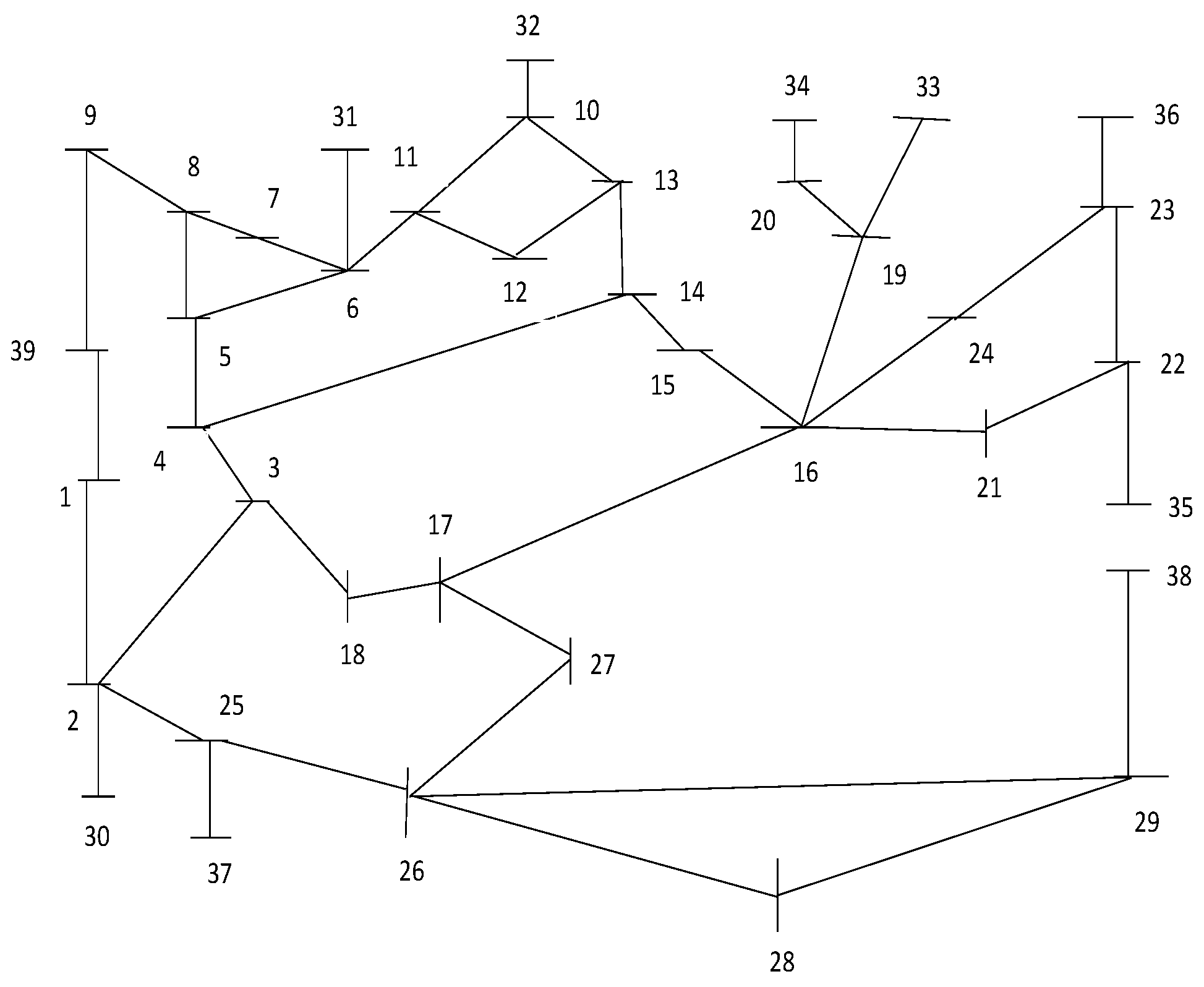
Test case: To test the above-mentioned algorithmic procedure in practice, we apply it to a 39-bus network case which is based on the New England system from the technical report [56] and from Alvarado et al. [57], and Hu and Ralph [23]. In this test system, the word “bus” stands for nodes such as generators and consumers. Originally the 39-bus network consists of 46 links and 39 nodes. This system is described as being typical of the New England electricity market; see Figure 6.1 in [56], and Figure 5 in Hu and Ralph [23], where 10 nodes represent the generators indicated by the bold dots and 17 nodes stands for the consumers displayed by the withdrawal arrows, and the remaining 12 nodes are reference nodes. Since, for simplicity, each node of our dynamic spot electricity market problem (11) only has a unique generator, we consider the 39-bus network to only have one generator at each node , and these generators play the role of players. This is indicated by small horizontal and vertical lines; see Figure 2. Moreover, every generator at each node w plays a non-cooperative game to maximize its own profit in the same way as mentioned in Section 5.
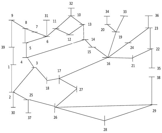
Figure 2.
The 39-bus test diagram based on the New England system.
Further, let and the multiple time parameters , where and are two moments of the given spot electricity market. We consider , and let be the piecewise smooth curve that links in . The constraint set of the ISO problem is given as
For and , we consider the following functional:
Now, for all p and , we have
From the above expression, it is clear that if , then the functional is strictly convex on the constraint set for each w, a fact which implies that is also strictly convex for on the constraint set . Consequently, the objective function of the ISO problem is strictly convex and, moreover, the constraint set is convex. Hence, the ISO’s optimization problem (10) has a unique solution, i.e., is a singleton set. In this way, the dynamic spot electricity market problem (the generator’s problem) (11) has a single value for p. Moreover, the cost functional of the DGNEP in the terms of dynamic spot electricity market problem (11) of Section 5 is given as

Table 1.
Numerical results ().
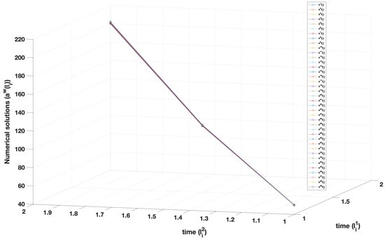
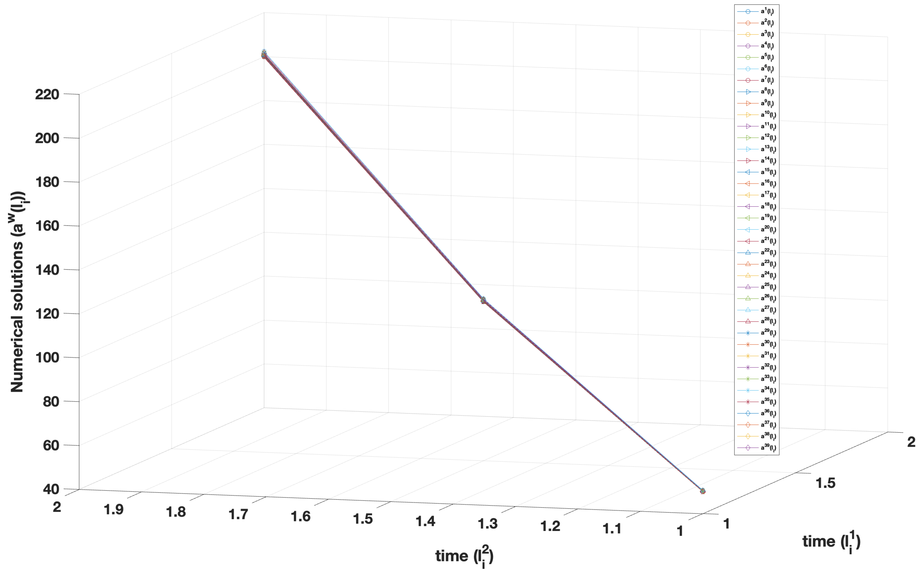
Figure 3.
Curves of equilibria for .
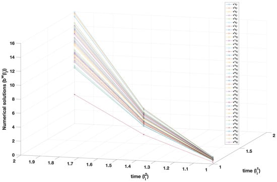
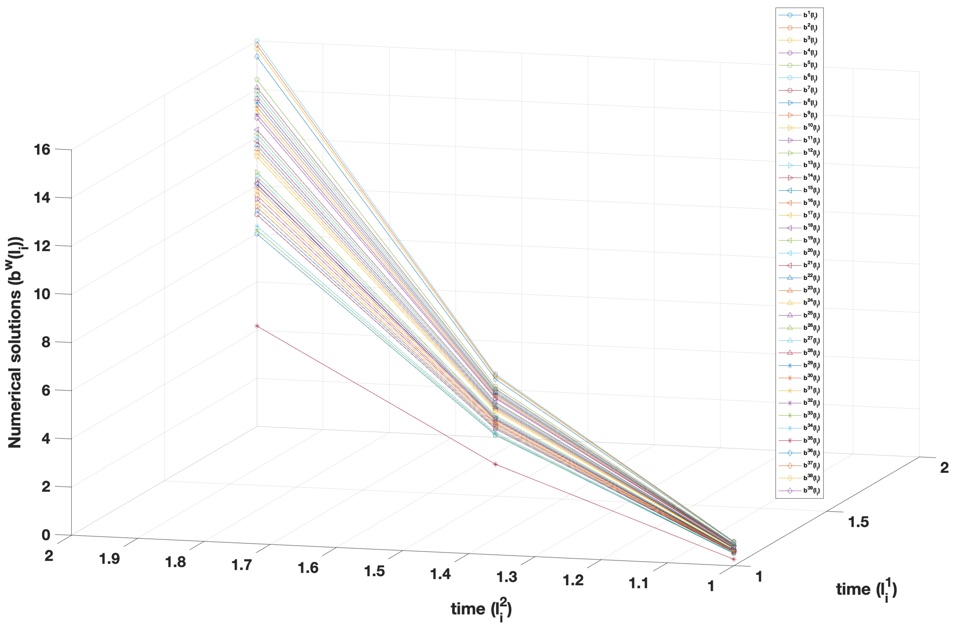
Figure 4.
Curves of equilibria for .
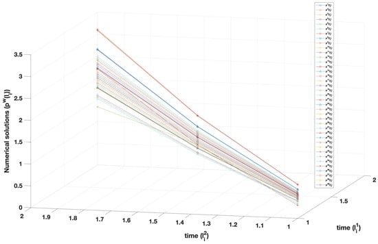
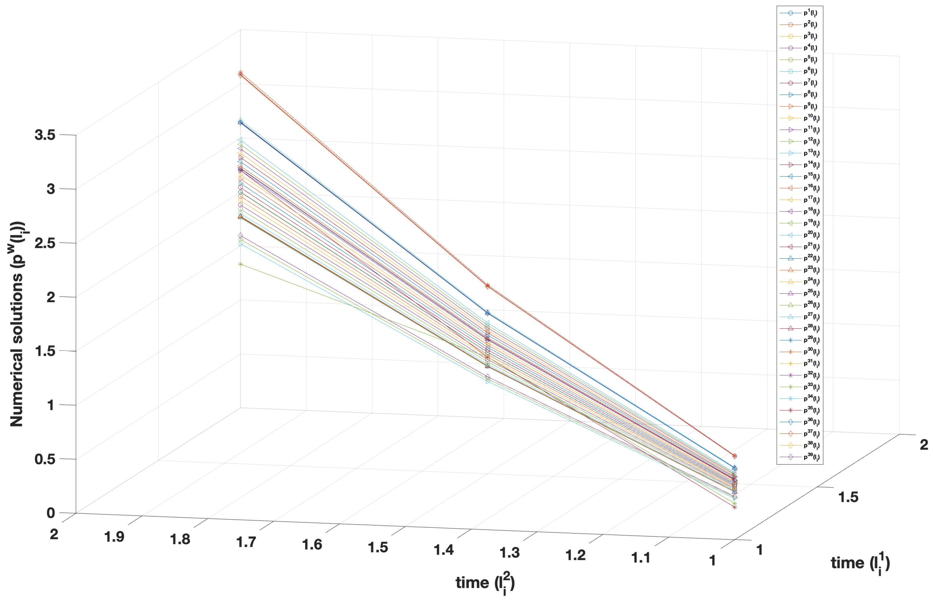
Figure 5.
Curves of equilibria for .

Table 2.
Curve of equilibria , for .

Table 3.
Numerical results ().
8. A Comparative Study
This section deals with the following question: “why do we need to consider multiple parameters of evolution instead of single parameter of evolution?”. In order to answer this question, we are going to compare our DGNEP with the single time-dependent generalized Nash equilibrium problem by solving the dynamic spot electricity market problem (11) and the dynamic spot electricity market problem of Aussel et al. [14] in terms of a simple numerical illustration. In the test case, we perform the numerical experiments for 39 generators. However, for the sake of simplicity, in this section we perform the numerical experiments only for three generators.
Case 1. We use the terminologies of Section 5 for three generators, and define the two-time parameters of evolution and as in the test case of Section 7. We consider the arguments of Section 5 for each as follows:
We have already observed in Section 7 that is a singleton if . For simplicity of the calculations, in this section, we will also perform the numerical experiments for . The dynamic spot electricity market problem is that each generator aims to maximize its profit by solving (11) in the sense of DGNEP. It is not difficult to prove that, for generator , , and , respectively, are the equilibria of (11). Now, for calculating the maximum profit of each generator, we consider the piecewise smooth curve as a straight line connecting the diagonals points and , i.e., for . For , the maximum profit of the generator can be calculated as follows:
Similarly, for the generators , their maximum profit can be calculated and the relevant values are and 822, respectively.
Case 2. We assume the multiple parameters of evolution t reduce to a single parameter of evolution, i.e., , , and that is simply a closed interval . Now, our formulated dynamic spot electricity market problem (11) becomes the dynamic spot electricity market problem of [14]. We have the corresponding arguments of Case 1, for each generator , as follows:
It is not difficult to calculate that for the generators , , and , respectively, are the equilibria of the dynamic spot electricity market problem of [14]. For , the maximum profit of the generator can be calculated as follows:
Similarly, for the generators , their maximum profit can be calculated and the relevant values are and , respectively.
This shows conclusively that the maximum profit value of each generator in the case of two-time parameters of evolution is higher than the corresponding value in the single time parameter of evolution case. This brings out the necessity and the advantage of formulating our DGNEP.
9. Conclusions and Further Developments
This paper is concerned with the areas of non-cooperative games and electricity market problems. We formulated a dynamic generalized Nash equilibrium problem and a dynamic quasi-variational inequality problem. We proved an equivalence between these two problems, as well as the existence of equilibria. Furthermore, as an application of our dynamic generalized Nash equilibrium problem, we reformulated a spot electricity market problem in the terms of such a problem. Moreover, we also presented a numerical method for solving the reformulated dynamic spot electricity market problem by using the theory of projected dynamical systems, and numerically solved a 39-bus network which is based on the New England system. We also presented a numerical experiment comparing the resulting payoffs of the multiple parameters and the single parameter cases.
The model developed in this paper provides a foundation for future studies that attempt to test the numerical comparison between the resulting payoffs/cost of GNEP in single and multiple time settings on the bigger and real-world data level. Our future research will also include the extension of the framework developed in the present paper to the supply chain network problems studied by Nagureny’s research group [12,21,28,31].
Author Contributions
Methodology, S.S., A.G. and S.R.; formal analysis, S.S., A.G. and S.R.; writing—review and editing, S.S., A.G. and S.R. All authors have read and agreed to the published version of the manuscript.
Funding
S.S. was financially supported by an European Research Consortium for Informatics and Mathematics (ERCIM) Alain Bensoussan postdoctoral fellowship. S.R. was partially supported by the Israel Science Foundation (Grant No. 820/17), by the Fund for the Promotion of Research at the Technion (Grant 2001893) and by the Technion General Research Fund (Grant 2016723).
Data Availability Statement
Dataset available on request from the authors.
Acknowledgments
All the authors are very grateful to two anonymous referees for their useful comments and helpful suggestions.
Conflicts of Interest
The authors declare no conflicts of interest.
References
- Neumann, J.V.; Morgenstern, O. Theory of Games and Economic Behavior; Princeton University Press: Princeton, NJ, USA, 1944. [Google Scholar]
- Nash, J.F. The bargaining problem. Econometrica 1950, 18, 155–162. [Google Scholar] [CrossRef]
- Nash, J.F. Two-person cooperative games. Econometrica 1953, 21, 128–140. [Google Scholar] [CrossRef]
- Cournot, A.A. Recherches sur les Principes Mathématiques de la Théorie des Richesses; Hachette: Paris, France, 1838. [Google Scholar]
- Nash, J.F. Equilibrium points in n-person games. Proc. Natl. Acad. Sci. USA 1950, 36, 48–49. [Google Scholar] [CrossRef] [PubMed]
- Nash, J.F. Non-cooperative games. Ann. Math. 1951, 54, 286–295. [Google Scholar] [CrossRef]
- Arrow, K.J.; Debreu, G. Existence of an equilibrium for a competitive economy. Econometrica 1954, 22, 265–290. [Google Scholar] [CrossRef]
- Facchinei, F.; Kanzow, C. Generalized Nash equilibrium problems. Ann. Oper. Res. 2010, 175, 177–211. [Google Scholar] [CrossRef]
- Fischer, A.; Herrich, M.; Schönefeld, K. Generalized Nash equilibrium problems-recent advances and challenges. Pesqui. Oper. 2014, 34, 521–558. [Google Scholar] [CrossRef]
- Britzelmeier, A.; Gerdts, M.; Rottmann, T. Control of interacting vehicles using model-predictive control, generalized Nash equilibrium problems, and dynamic inversion. IFAC PapersOnLine 2020, 53, 15146–15153. [Google Scholar] [CrossRef]
- Cadrea, H.L.; Jacquot, P.; Wan, C.; Alasseur, C. Peer-to-peer electricity market analysis: From variational to Generalized Nash Equilibrium. Eur. J. Oper. Res. 2020, 282, 753–771. [Google Scholar] [CrossRef]
- Nagurney, A.; Dutta, P. Supply chain network competition among blood service organizations: A Generalized Nash Equilibrium framework. Ann. Oper. Res. 2019, 275, 551–586. [Google Scholar] [CrossRef]
- Nagurney, A.; Flores, E.A.; Soylu, C. A Generalized Nash Equilibrium network model for post-disaster humanitarian relief. Transp. Res. Part E 2016, 95, 1–18. [Google Scholar] [CrossRef]
- Aussel, D.; Gupta, R.; Mehra, A. Evolutionary variational inequality formulation of the generalized Nash equilibrium problem. J. Optim. Theory Appl. 2016, 169, 74–90. [Google Scholar] [CrossRef]
- Cotrina, J.; Ziga, J. Time-Dependent Generalized Nash Equilibrium Problem. J. Optim. Theory Appl. 2018, 179, 1054–1064. [Google Scholar] [CrossRef]
- Bensoussan, A. Points de Nash dans le cas de fontionnelles quadratiques et jeux differentiels linéaires à N personnes. SIAM J. Control 1974, 12, 460–499. [Google Scholar] [CrossRef]
- Harker, P.T. Generalized Nash games and quasi-variational inequalities. Eur. J. Oper. Res. 1991, 54, 81–94. [Google Scholar] [CrossRef]
- Aussel, D.; Sultana, A.; Vetrivel, V. On the existence of projected solutions of quasi-variational inequalities and generalized Nash equilibrium problems. J. Optim. Theory Appl. 2016, 170, 818–837. [Google Scholar] [CrossRef]
- Bueno, O.; Cotrina, J. Existence of Projected Solutions for Generalized Nash Equilibrium Problems. J. Optim. Theory Appl. 2021, 191, 344–362. [Google Scholar] [CrossRef]
- Cotrina, J.; Ziga, J. Quasi-equilibrium problems with non-self constraint map. J. Glob. Optim. 2019, 75, 177–197. [Google Scholar] [CrossRef]
- Nagurney, A. Supply chain game theory network modeling under labor constraints: Applications to the COVID-19 pandemic. Eur. J. Oper. Res. 2021, 293, 880–891. [Google Scholar] [CrossRef]
- Nagurney, A.; Salarpour, M.; Dong, J.; Dutta, P. Competition for Medical Supplies Under Stochastic Demand in the Covid-19 Pandemic: A Generalized Nash Equilibrium Framework. In Nonlinear Analysis and Global Optimization; Themistocles M. Rassias, T.M., Pardalos, P.M., Eds.; Springer: Berlin/Heidelberg, Germany, 2021. [Google Scholar] [CrossRef]
- Hu, X.; Ralph, D. Using EPECs to model bilevel games in restructured electricity markets with locational prices. Oper. Res. 2007, 55, 809–827. Available online: http://www.jstor.org/stable/25147124 (accessed on 1 July 2024). [CrossRef]
- Aussel, D.; Correa, R.; Marechal, M. Electricity spot market with transmission losses. J. Ind. Manag. Optim. 2013, 9, 275–290. [Google Scholar] [CrossRef]
- Berry, C.A.; Hobbs, B.F.; Meroney, W.A.; O’Neill, R.P.; Stewart, W.R., Jr. Understanding how market power can arise in network competition: A game theoretic approach. Util. Policy 1999, 8, 139–158. [Google Scholar] [CrossRef]
- Escobar, J.F.; Jofré, A. Monopolistic competition in electricity networks with resistance losses. Econ. Theory 2010, 44, 101–121. [Google Scholar] [CrossRef][Green Version]
- Hobbs, B.J.; Member Metzler, C.B.; Pang, J.-S. Strategic gaming analysis for electric power systems: An MPEC approach. IEEE Trans. Power Syst. 2000, 15, 638–645. [Google Scholar] [CrossRef]
- Nagurney, A.; Matsypura, D. A Supply Chain Network Perspective for Electric Power Generation, Supply, Transmission, and Consumption. In Optimisation, Econometric and Financial; Kontoghiorghes, E.J., Gatu, C., Eds.; Springer: Berlin/Heidelberg, Germany; New York, NY, USA, 2007. [Google Scholar] [CrossRef]
- Henry, C. An existence theorem for a class of differential equations with multivalued right-hand side. J. Math. Anal. Appl. 1973, 41, 179–186. [Google Scholar] [CrossRef]
- Nagurney, A.; Zhang, D. Projected Dynamical Systems and Variational Inequalities with Applications; Springer: New York, NY, USA, 1996. [Google Scholar] [CrossRef]
- Nagurney, A.; Liu, Z.; Cojocaru, M.-G.; Daniele, P. Dynamic electric power supply chains and transportation networks: An evolutionary variational inequality formulation. Transp. Res. Part E 2007, 43, 624–646. [Google Scholar] [CrossRef]
- Cojocaru, M.G.; Daniele, P.; Nagurney, A. Projected dynamical systems and evolutionary variational inequalities via Hilbert spaces with applications. J. Optim. Theory Appl. 2005, 127, 549–563. [Google Scholar] [CrossRef]
- Cojocaru, M.G.; Daniele, P.; Nagurney, A. Double-layered dynamics: A unified theory of projected dynamical systems and evolutionary variational inequalities. Eur. J. Oper. Res. 2006, 175, 494–507. [Google Scholar] [CrossRef]
- Cojocaru, M.G.; Daniele, P.; Nagurney, A. Projected dynamical systems, evolutinary variational inequalities, applications, and a computational procedure. In Pareto Optimality, Game Theory and Equilibria; Springer: New York, NY, USA, 2006. [Google Scholar] [CrossRef]
- Cojocaru, M.G.; Jonker, L.B. Existence of solutions to projected differential equations in Hilbert spaces. Proc. Am. Math. Soc. 2004, 132, 183–193. [Google Scholar] [CrossRef]
- Migot, T.; Cojocaru, M.-G. Nonsmooth dynamics of generalized Nash games. J. Nonlinear Var. Anal. 2020, 4, 27–44. [Google Scholar] [CrossRef]
- Ekeland, I.; Témam, R. Convex Analysis and Variational Problems; North-Holland: Amsterdam, The Netherlands, 1976. [Google Scholar]
- Guseĭnov, F.V. On the question of extension of multidimensional variational problems. Math. USSR-Izv. 1987, 28, 1–19. [Google Scholar] [CrossRef]
- Fonseca, I.; Marcellini, P. Relaxation of Multiple Integrals in Subcritical Sobolev Spaces. J. Geom. Anal. 1997, 7, 57–81. [Google Scholar] [CrossRef]
- Hüsseinov, F. Relaxation of multidimensional variational problems with constraints of general form. Nonlinear Anal. 2001, 45, 651–659. [Google Scholar] [CrossRef]
- Pickenhain, S.; Wagner, M. Pontryagin principle for state-constrained control problems governed by a first-order PDE system. J. Optim. Theory Appl. 2000, 107, 297–330. [Google Scholar] [CrossRef]
- Pickenhain, S.; Wagner, M. Piecewise continuous controls in Dieudonne-Rashevsky type problems. J. Optim. Theory Appl. 2005, 127, 145–163. [Google Scholar] [CrossRef]
- Wagner, M. Pontryagin’s maximum principle for Dieudonné-Rashevsky type problems involving lipschitz functions. Optimization 1999, 46, 165–184. [Google Scholar] [CrossRef]
- Wagner, M. Pontryagin’s Maximum Principle for multidimensional control problems in image processing. J. Optim. Theory Appl. 2009, 140, 543–576. [Google Scholar] [CrossRef]
- Udrişte, C.; Ţevy, I. Multi-time Euler-Lagrange-Hamilton theory. WSEAS Trans. Math. 2007, 6, 701–709. [Google Scholar]
- Udrişte, C. Multitime controllability, observability and bang-bang principle. J. Optim. Theory Appl. 2008, 139, 141–157. [Google Scholar] [CrossRef]
- Udrişte, C.; Dogaru, O.; Ţevy, I. Null Lagrangian forms and Euler-Lagrange PDEs. J. Adv. Math. Study 2008, 1, 143–156. [Google Scholar]
- Udrişte, C.; Ferrara, M. Multitime models of optimal growth. WSEAS Trans. Math. 2008, 7, 51–55. [Google Scholar]
- Singh, S.; Pitea, A.; Qin, X. An iterative method and weak sharp solutions for multitime-type variational inequalities. Appl. Anal. 2021, 302, 265–287. [Google Scholar] [CrossRef]
- Treanţă, S.; Singh, S. Weak sharp solutions associated with a multidimensional variational-type inequality. Positivity 2021, 25, 329–351. [Google Scholar] [CrossRef]
- Ansari, Q.H.; Schaible, S.; Yao, J.C. Generalized vector quasi-variational inequality problems over product sets. J. Glob. Optim. 2005, 32, 437–449. [Google Scholar] [CrossRef]
- Ding, X.P. Existence of solutions for quasi-equilibrium problems in noncompact topological spaces. Comput. Math. Appl. 2000, 39, 13–21. [Google Scholar] [CrossRef]
- Pang, J.S.; Fukushima, M. Quasi-variational inequalities, generalized Nash equilibria, and multi-leader-follower games. Comput. Manag. Sci. 2005, 2, 21–56. [Google Scholar] [CrossRef]
- Hanson, M.A. Bounds for functionally convex optimal control problems. J. Math. Anal. Appl. 1964, 8, 84–89. [Google Scholar] [CrossRef]
- Singh, S.; Gibali, G.; Reich, S. Multi-time generalized Nash equilibria with dynamic flow applications. Mathematics 2021, 9, 1658. [Google Scholar] [CrossRef]
- Alvarado, F.L.; Demarco, C.L.; Dobson, I.; Sauer, P.W.; Greene, S.; Engdahl, H.; Zhang, J. Electric Power Transfer Capability: Concepts, Applications, Sensitivity and Uncertainty. March 2001. Available online: https://www.researchgate.net/publication/2892623 (accessed on 1 July 2024).
- Alvarado, F.L.; Meng, J.; Demarco, C.L.; Mota, W.S. Stability analysis of interconnected power systems coupled with market dynamics. IEEE Trans. Power Syst. 2001, 16, 695–701. [Google Scholar] [CrossRef]
- Svendsen, A.; Boutilier, R.G.; Abbott, R.M.; Wheeler, D. Measuring the Business Value of Stakeholder Relationships (Part One). Available online: https://partnersinchange.co.nz/wp-content/uploads/2017/10/Canadian-Measuring-the-value-of-Stakeholder-relationships.pdf (accessed on 1 July 2024).
- Cruz, J.M.; Liu, Z. Modeling and analysis of the multiperiod effects of social relationship on supply chain networks. Eur. J. Oper. Res. 2011, 214, 39–52. [Google Scholar] [CrossRef]
- Cruz, J.M.; Wakolbinger, T. Multiperiod effects of corporate social responsibility on supply chain networks, transaction costs, emissions, and risk. Int. J. Prod. Econ. 2008, 116, 61–74. [Google Scholar] [CrossRef]
- Treanţă, S. On a modified optimal control problem with first-order PDE constraints and the associated saddle-point optimality criterion. Eur. J. Control 2020, 51, 1–9. [Google Scholar] [CrossRef]
- Jayswal, A.; Singh, S.; Kurdi, A. Multitime multiobjective variational problems and vector variational-like inequalities. Eur. J. Oper. Res. 2016, 254, 739–745. [Google Scholar] [CrossRef]
- Mititelu, Ş.; Treanţă, S. Efficiency conditions in vector control problems governed by multiple integrals. J. Appl. Math. Comput. 2018, 57, 647–665. [Google Scholar] [CrossRef]
- Singh, S.; Reich, S. A multidimensional approach to traffic analysis. Pure Appl. Funct. Anal. 2021, 6, 383–397. [Google Scholar]
- Matsushita, S.-Y.; Xu, L. On finite convergence of iterative methods for variational inequalities in Hilbert spaces. J. Optim. Theory Appl. 2014, 161, 701–715. [Google Scholar] [CrossRef]
- Cegielski, A. Iterative Methods for Fixed Point Problems in Hilbert Spaces; Springer: Berlin/Heidelberg, Germany, 2012. [Google Scholar]
- Rockafellar, R.T.; Wets, R.J.-B. Variational Analysis; Springer Science & Business Media: Berlin/Heidelberg, Germany, 2009. [Google Scholar]
- Saadat, H. Power System Analysis; McGraw-Hill: Boston, MA, USA, 1999. [Google Scholar]
Disclaimer/Publisher’s Note: The statements, opinions and data contained in all publications are solely those of the individual author(s) and contributor(s) and not of MDPI and/or the editor(s). MDPI and/or the editor(s) disclaim responsibility for any injury to people or property resulting from any ideas, methods, instructions or products referred to in the content. |
© 2024 by the authors. Licensee MDPI, Basel, Switzerland. This article is an open access article distributed under the terms and conditions of the Creative Commons Attribution (CC BY) license (https://creativecommons.org/licenses/by/4.0/).


