Several Characterizations of the Generalized 1-Parameter 3-Variable Hermite Polynomials

Abstract

This paper presents a novel framework for introducing generalized 1-parameter 3-variable Hermite polynomials. These polynomials are characterized through generating functions and series definitions, elucidating their fundamental properties. Moreover, utilising a factorisation method, this study establishes recurrence relations, shift operators, and various differential equations, including differential, integro-differential, and partial differential equations.

1. Introduction and Preliminaries

In recent years, notable progress has been made in developing various generalizations of special functions within mathematical physics. These advancements provide a robust analytical framework for solving various mathematical physics problems and have extensive practical applications across diverse domains. Particularly, the significance of generalized Hermite polynomials has been underscored, as noted in previous studies [1,2,3]. These polynomials find utility in addressing challenges in quantum mechanics, optical beam transport, and a spectrum of problems spanning partial differential equations to abstract group theory.

The “2-variable Hermite Kampé de Feriet polynomials (2VHKdFP)”, denoted as ${\mathcal{Q}}_n({\lambda }_1,{\lambda }_2)$ [4], are expressed through the following generating function:

$$e^{{\lambda }_1\Omega +{\lambda }_2{\Omega }^2}=\sum _{n=0}^{\infty }{\mathcal{Q}}_n({\lambda }_1,{\lambda }_2){\displaystyle \frac{{\Omega }^n}{n!}},$$

(1)

which for ${\lambda }_2=0$, gives

$$e^{{\lambda }_1\Omega }=\sum _{n=0}^{\infty }{\mathcal{Q}}_n\left({\lambda }_1\right){\displaystyle \frac{{\Omega }^n}{n!}}.$$

(2)

Similarly, the “2-variable 1-parameter Hermite polynomials (2V1PHP)”, represented as ${\mathcal{Q}}_n({\lambda }_1,{\lambda }_2,\mathcal{C})$, are defined using the subsequent generating function [5]:

$${\mathcal{C}}^{{\lambda }_1\Omega +{\lambda }_2{\Omega }^2}=\sum _{n=0}^{\infty }{\mathcal{Q}}_n({\lambda }_1,{\lambda }_2,\mathcal{C}){\displaystyle \frac{{\Omega }^n}{n!}},\mathcal{C}>1,$$

(3)

which for ${\lambda }_2=0$ reduces to

$${\mathcal{C}}^{{\lambda }_1\Omega }=\sum _{n=0}^{\infty } {\mathbb{R}}_n({\lambda }_1,\mathcal{C}){\displaystyle \frac{{\Omega }^n}{n!}},\mathcal{C}>1.$$

(4)

The “3-variable Hermite polynomials (3VHP)”, denoted as ${\mathcal{Q}}_n({\lambda }_1,{\lambda }_2,{\lambda }_3)$ [6], are characterized by the following generating function:

$$e^{{\lambda }_1\Omega +{\lambda }_2{\Omega }^2+{\lambda }_3{\Omega }^3}=\sum _{n=0}^{\infty } {\mathcal{Q}}_n({\lambda }_1,{\lambda }_2,{\lambda }_3){\displaystyle \frac{{\Omega }^n}{n!}}.$$

(5)

The orthogonality of Hermite polynomials is crucial in various fields, such as quantum mechanics, probability theory, and numerical analysis. In quantum mechanics, they form the basis for the wave functions of the quantum harmonic oscillator, ensuring the orthogonality and completeness needed for accurate probability calculations. In probability theory, they are key in studying Gaussian distributions and polynomial chaos expansions. Additionally, they play a significant role in signal processing and are eigenfunctions of the Fourier transform, making them indispensable in theoretical and applied mathematics. In their 3-variable formulation, these polynomials find widespread application across numerous fields in both pure and applied mathematics and physics. They serve as fundamental tools in addressing problems ranging from Laplace’s equation in parabolic coordinates to various quantum mechanics and probability theory scenarios. Notably, for any integral value of n, these polynomials represent specific solutions to the heat or generalized heat problem facilitated by the corresponding existence of Gauss–Weierstrass transforms.

Consider ${\left\{{\varphi }_n\left({\lambda }_1\right)\right\}}_{n=0}^{\infty }$, which signifies a series of polynomials; we can observe that $\mathrm{deg}\left({\varphi }_n\left({\lambda }_1\right)\right)=n,(n\in {\mathbb{N}}_0:=\{0,1,2,\cdots \}$. The differential operators ${\Psi }_n^{-}$ and ${\Psi }_n^{+}$ meeting the criteria

$${\Psi }_n^{-}\left\{{\varphi }_n\left({\lambda }_1\right)\right\}={\varphi }_{n-1}\left({\lambda }_1\right),$$

(6)

$${\Psi }_n^{+}\left\{{\varphi }_n\left({\lambda }_1\right)\right\}={\varphi }_{n+1}\left({\lambda }_1\right)$$

(7)

are referred to as multiplicative and derivative operators, in turn. ${\left\{{\varphi }_n\left({\lambda }_1\right)\right\}}_{n=0}^{\infty }$ is a series of polynomials that are considered quasi-monomial if and only if Equations (6) and (7) hold. A differential equation like this can be found by finding the derivative and multiplicative operators for a given polynomial family as

$$\left({\Psi }_{n+1}^{-}{\Psi }_n^{+}\right)\left\{{\varphi }_n\left({\lambda }_1\right)\right\}={\varphi }_n\left({\lambda }_1\right).$$

(8)

The factorization technique is the name given to this process. Determining the multiplicative operator ${\Psi }_n^{+}$ and the derivative operator ${\Psi }_n^{-}$ forms the basis of the factorization approach [7,8,9,10,11,12,13,14,15]. The monomiality principle is another way to think about this method. When the factorization approach is applied to the domain of multivariable special functions, new analytical techniques are presented to solve a wide variety of partial differential equations frequently encountered in practical situations.

Differential equations cover a wide range of topics in “physics, engineering, and pure and applied mathematics”. Problems from various scientific and technical fields typically take the form of differential equations, solved using specialised functions. Differential equation theory has attracted renewed attention in the last thirty years due to developments in nonlinear analysis, dynamical systems, and their useful applications in science and engineering.

Several studies employing different generating function approaches and analytical procedures have been carried out to present and analyse hybrid families of special polynomials methodically [16,17]. The recurrence relations, explicit relations, functional and differential equations, summation formulae, and symmetric and convolution identities are just a few of the fundamental characteristics of multi-variable hybrid special polynomials that make them important. “Number theory, combinatorics, classical and numerical analysis, theoretical physics, approximation theory, and other fields of pure and practical mathematics” are just a few of the fields in which these polynomials can be useful to researchers. Various scientific areas can use the qualities of hybrid special polynomials to address new problems.

The article is organised as follows: Section 2 overviews the 3-variable 1-parameter generalized Hermite polynomials utilizing series definitions and generating functions. It also describes how to derive the related differential, integro-differential, and partial differential equations. Section 3 examines particular instances from this polynomial family to demonstrate the usefulness of the major conclusions. Section 4 investigates specific cases of the 1-parameter, 3-variable, generalized Hermite polynomials. Finally, the last part contains closing thoughts.

2. Polynomials Based on Generalized Hermite Polynomials with One Parameter and Three Variables

This section introduces a hybrid family known as the generalized 1-parameter 3-variable Hermite polynomials (G-1P3-VHP) via the following generating relation:

$${\mathcal{C}}^{{\lambda }_1\Omega +{\lambda }_2{\Omega }^2+{\lambda }_3{\Omega }^3}=\sum _{n=0}^{\infty } {\mathcal{Q}}_n({\lambda }_1,{\lambda }_2,{\lambda }_3;\mathcal{C}){\displaystyle \frac{{\Omega }^n}{n!}},\mathcal{C}>1,$$

The definition is proven in Theorem 2.1. Additionally, various properties of these polynomials are established. To obtain the generating function for the G-1P3-VHP, a key result is demonstrated as follows:

Theorem 1.

For the G-1P3-VHP ${\mathcal{Q}}_n({\lambda }_1,{\lambda }_2,{\lambda }_3;\mathcal{C})$, the following generating relation is demonstrated:

$${\mathcal{C}}^{{\lambda }_1\Omega +{\lambda }_2{\Omega }^2+{\lambda }_3{\Omega }^3}=\sum _{n=0}^{\infty } {\mathcal{Q}}_n({\lambda }_1,{\lambda }_2,{\lambda }_3;\mathcal{C}){\displaystyle \frac{{\Omega }^n}{n!}},\mathcal{C}>1,$$

(9)

or, equivalently

$$e^{\ln \mathcal{C}({\lambda }_1\Omega +{\lambda }_2{\Omega }^2+{\lambda }_3{\Omega }^3)}=\sum _{n=0}^{\infty } {\mathcal{Q}}_n({\lambda }_1,{\lambda }_2,{\lambda }_3;\mathcal{C}){\displaystyle \frac{{\Omega }^n}{n!}},\mathcal{C}>1.$$

(10)

Proof. 

Substituting the exponents of $\Omega$, i.e., ${\lambda }_1^0,{\lambda }_1^1,{\lambda }_1^2,\cdots ,{\lambda }_1^n$ in the expansion of $e^{{\lambda }_1\Omega }$ by the polynomials ${\mathcal{Q}}_0({\lambda }_1,{\lambda }_2,{\lambda }_3;\mathcal{C}), {\mathcal{Q}}_2({\lambda }_1,{\lambda }_2,{\lambda }_3;\mathcal{C})$, $\cdots , {\mathcal{Q}}_n({\lambda }_1,{\lambda }_2,{\lambda }_3;\mathcal{C})$ in the left hand part and ${\lambda }_1$ by ${\mathcal{Q}}_n({\lambda }_1,{\lambda }_2,{\lambda }_3;\mathcal{C})$ in the right hand part of the expression (2), which indicates the resulting G-1P3-VHP in the right hand side, leading to (9). The generating function (10) is obtained by simplifying the left-hand side of Equation (9). □

The following theorem gives the series definition for the G-1P3-VHP ${\mathcal{Q}}_n({\lambda }_1,{\lambda }_2,{\lambda }_3;\mathcal{C})$:

Theorem 2.

For the G-1P3-VHP ${\mathcal{Q}}_n({\lambda }_1,{\lambda }_2,{\lambda }_3;\mathcal{C})$, the following series representation is demonstrated:

$${\mathcal{Q}}_n({\lambda }_1,{\lambda }_2,{\lambda }_3;\mathcal{C})=n!\sum _{k=0}^{[n/3]}{\displaystyle \frac{{\mathcal{Q}}_{n-3k}({\lambda }_1,{\lambda }_2){\lambda }_3^k}{(n-3k)!k!}}{\left(\ln \mathcal{C}\right)}^{n-2k}.$$

(11)

Proof. 

Inserting the expressions (3) and the expansion of $e^{\ln \mathcal{C}\left({\lambda }_3{\Omega }^3\right)}$ in left hand part of the expression (5), it follows that

$$\sum _{n=0}^{\infty } {\mathcal{Q}}_n({\lambda }_1,{\lambda }_2,{\lambda }_3;\mathcal{C}){\displaystyle \frac{{\Omega }^n}{n!}}=\sum _{n=0}^{\infty }{ \mathcal{Q}}_n({\lambda }_1,{\lambda }_2){\displaystyle \frac{{(\ln \mathcal{C}\Omega )}^n}{n!}}\sum _{k=0}^{\infty }{\lambda }_3^k{\displaystyle \frac{{\left(\ln \mathcal{C}{\Omega }^3\right)}^k}{k!}},$$

(12)

thus, operating the Cauchy-product rule

$$\sum _{n=0}^{\infty }\sum _{k=0}^{\infty }\mathcal{A}(n,k)=\sum _{n=0}^{\infty }\sum _{k=0}^{\left[{\displaystyle \frac{n}{3}}\right]}\mathcal{A}(n-3k,k)$$

yields the expression:

$$\sum _{n=0}^{\infty } {\mathcal{Q}}_n({\lambda }_1,{\lambda }_2,{\lambda }_3;\mathcal{C}){\displaystyle \frac{{\Omega }^n}{n!}}=n!\sum _{n=0}^{\infty }\sum _{k=0}^{[n/3]}{\displaystyle \frac{{\mathcal{Q}}_{n-3k}({\lambda }_1,{\lambda }_2){\lambda }_3^k}{(n-3k)!k!}}{\left(\ln \mathcal{C}\right)}^{n-2k}{\displaystyle \frac{{\Omega }^n}{n!}}.$$

(13)

Assertion (11) is obtained by comparing the coefficients of the identical powers of $\Omega$ on both sides of the above expression. □

For $\mathcal{C}=1.5,2,2.5,3$, the first six G-1P3-VHP ${\mathcal{Q}}_n({\lambda }_1,{\lambda }_2,{\lambda }_3;\mathcal{C})$ are given as:

$$\begin{array}{ccc}\hfill {\mathcal{Q}}_0\left({\lambda }_1,{\lambda }_2,{\lambda }_3;1.5\right)& =& 1,\hfill \\ \hfill {\mathcal{Q}}_1\left({\lambda }_1,{\lambda }_2,{\lambda }_3;1.5\right)& =& 0.405465{\lambda }_1,\hfill \\ \hfill {\mathcal{Q}}_2\left({\lambda }_1,{\lambda }_2,{\lambda }_3;1.5\right)& =& 0.082201\left(1.{\lambda }_1^2+4.93261{\lambda }_2\right),\hfill \\ \hfill {\mathcal{Q}}_3\left({\lambda }_1,{\lambda }_2,{\lambda }_3;1.5\right)& =& 0.0111099\left(1.{\lambda }_1^3+14.7978{\lambda }_1{\lambda }_2+36.4959{\lambda }_3\right),\hfill \\ \hfill {\mathcal{Q}}_4\left({\lambda }_1,{\lambda }_2,{\lambda }_3;1.5\right)& =& 0.082201\left(0.0137002{\lambda }_1^4+0.405465{\lambda }_1^2{\lambda }_2+1.{\lambda }_2^2+2.{\lambda }_1{\lambda }_3\right),\hfill \\ \hfill {\mathcal{Q}}_5\left({\lambda }_1,{\lambda }_2,{\lambda }_3;1.5\right)& =& 0.0000913243\left(1.{\lambda }_1^5+49.3261{\lambda }_1^3{\lambda }_2+364.959{\lambda }_1{\lambda }_2^2+364.959{\lambda }_1^2{\lambda }_3+1800.2{\lambda }_2{\lambda }_3\right),\hfill \\ \hfill {\mathcal{Q}}_6\left({\lambda }_1,{\lambda }_2,{\lambda }_3;1.5\right)& =& 0.082201\left(0.0000750778{\lambda }_1^6+0.00555494{\lambda }_1^4{\lambda }_2+0.082201{\lambda }_1^2{\lambda }_2^2+0.135155{\lambda }_2^3+0.0548007{\lambda }_1^3{\lambda }_3\right)\hfill \\ & & +0.082201\left(0.81093{\lambda }_1{\lambda }_2{\lambda }_3+{\lambda }_3^2\right).\hfill \end{array}$$

$$\begin{array}{ccc}\hfill {\mathcal{Q}}_0\left({\lambda }_1,{\lambda }_2,{\lambda }_3;2\right)& =& 1,\hfill \\ \hfill {\mathcal{Q}}_1\left({\lambda }_1,{\lambda }_2,{\lambda }_3;2\right)& =& {\lambda }_{1}log\left[2\right],\hfill \\ \hfill {\mathcal{Q}}_2\left({\lambda }_1,{\lambda }_2,{\lambda }_3;2\right)& =& {\displaystyle \frac{1}{2}}\left(2{\lambda }_{2}log\left[2\right]+{\lambda }_1^{2}log{\left[2\right]}^2\right),\hfill \\ \hfill {\mathcal{Q}}_3\left({\lambda }_1,{\lambda }_2,{\lambda }_3;2\right)& =& {\displaystyle \frac{1}{6}}\left(6{\lambda }_{3}log\left[2\right]+6{\lambda }_1{\lambda }_{2}log{\left[2\right]}^2+{\lambda }_1^{3}log{\left[2\right]}^3\right),\hfill \\ \hfill {\mathcal{Q}}_4\left({\lambda }_1,{\lambda }_2,{\lambda }_3;2\right)& =& {\displaystyle \frac{1}{24}}\left(12{\lambda }_2^{2}log{\left[2\right]}^2+24{\lambda }_1{\lambda }_{3}log{\left[2\right]}^2+12{\lambda }_1^2{\lambda }_{2}log{\left[2\right]}^3+{\lambda }_1^{4}log{\left[2\right]}^4\right),\hfill \\ \hfill {\mathcal{Q}}_5\left({\lambda }_1,{\lambda }_2,{\lambda }_3;2\right)& =& {\displaystyle \frac{1}{120}}\left(120{\lambda }_2{\lambda }_{3}log{\left[2\right]}^2+60{\lambda }_1{\lambda }_2^{2}log{\left[2\right]}^3+60{\lambda }_1^2{\lambda }_{3}log{\left[2\right]}^3+20{\lambda }_1^3{\lambda }_{2}log{\left[2\right]}^4+{\lambda }_1^{5}log{\left[2\right]}^5\right),\hfill \\ \hfill {\mathcal{Q}}_6\left({\lambda }_1,{\lambda }_2,{\lambda }_3;2\right)& =& {\displaystyle \frac{1}{720}}\left(360{\lambda }_3^{2}log{\left[2\right]}^2+120{\lambda }_2^{3}log{\left[2\right]}^3+720{\lambda }_1{\lambda }_2{\lambda }_{3}log{\left[2\right]}^3+180{\lambda }_1^2{\lambda }_2^{2}log{\left[2\right]}^4+120{\lambda }_1^3{\lambda }_{3}log{\left[2\right]}^4\right)\hfill \\ & & +{\displaystyle \frac{1}{720}}\left(30{\lambda }_1^4{\lambda }_{2}log{\left[2\right]}^5+{\lambda }_1^{6}log{\left[2\right]}^6\right).\hfill \end{array}$$

$$\begin{array}{ccc}\hfill {\mathcal{Q}}_0\left({\lambda }_1,{\lambda }_2,{\lambda }_3;2.5\right)& =& 1,\hfill \\ \hfill {\mathcal{Q}}_1\left({\lambda }_1,{\lambda }_2,{\lambda }_3;2.5\right)& =& 0.916291{\lambda }_1,\hfill \\ \hfill {\mathcal{Q}}_2\left({\lambda }_1,{\lambda }_2,{\lambda }_3;2.5\right)& =& 0.419794\left(1.{\lambda }_1^2+2.18271{\lambda }_2\right),\hfill \\ \hfill {\mathcal{Q}}_3\left({\lambda }_1,{\lambda }_2,{\lambda }_3;2.5\right)& =& 0.128218\left(1.{\lambda }_1^3+6.54814{\lambda }_1{\lambda }_2+7.14636{\lambda }_3\right),\hfill \\ \hfill {\mathcal{Q}}_4\left({\lambda }_1,{\lambda }_2,{\lambda }_3;2.5\right)& =& 0.419794\left(0.0699657{\lambda }_1^4+0.916291{\lambda }_1^2{\lambda }_2+1.{\lambda }_2^2+2.{\lambda }_1{\lambda }_3\right),\hfill \\ \hfill {\mathcal{Q}}_5\left({\lambda }_1,{\lambda }_2,{\lambda }_3;2.5\right)& =& 0.00538251\left(1.{\lambda }_1^5+21.8271{\lambda }_1^3{\lambda }_2+71.4636{\lambda }_1{\lambda }_2^2+71.4636{\lambda }_1^2{\lambda }_3+155.984{\lambda }_2{\lambda }_3\right),\hfill \\ \hfill {\mathcal{Q}}_6\left({\lambda }_1,{\lambda }_2,{\lambda }_3;2.5\right)& =& 0.419794\left(0.00195808{\lambda }_1^6+0.0641089{\lambda }_1^4{\lambda }_2+0.419794{\lambda }_1^2{\lambda }_2^2+0.30543{\lambda }_2^3+0.279863{\lambda }_1^3{\lambda }_3\right)\hfill \\ & & +0.419794\left(1.83258{\lambda }_1{\lambda }_2{\lambda }_3+{\lambda }_3^2\right).\hfill \end{array}$$

$$\begin{array}{ccc}\hfill {\mathcal{Q}}_0\left({\lambda }_1,{\lambda }_2,{\lambda }_3;3\right)& =& 1,\hfill \\ \hfill {\mathcal{Q}}_1\left({\lambda }_1,{\lambda }_2,{\lambda }_3;3\right)& =& {\lambda }_{1}log\left[3\right],\hfill \\ \hfill {\mathcal{Q}}_2\left({\lambda }_1,{\lambda }_2,{\lambda }_3;3\right)& =& {\displaystyle \frac{1}{2}}\left(2{\lambda }_{2}log\left[3\right]+{\lambda }_1^{2}log{\left[3\right]}^2\right),\hfill \\ \hfill {\mathcal{Q}}_3\left({\lambda }_1,{\lambda }_2,{\lambda }_3;3\right)& =& {\displaystyle \frac{1}{6}}\left(6{\lambda }_{3}log\left[3\right]+6{\lambda }_1{\lambda }_{2}log{\left[3\right]}^2+{\lambda }_1^{3}log{\left[3\right]}^3\right),\hfill \\ \hfill {\mathcal{Q}}_4\left({\lambda }_1,{\lambda }_2,{\lambda }_3;3\right)& =& {\displaystyle \frac{1}{24}}\left(12{\lambda }_2^{2}log{\left[3\right]}^2+24{\lambda }_1{\lambda }_{3}log{\left[3\right]}^2+12{\lambda }_1^2{\lambda }_{2}log{\left[3\right]}^3+{\lambda }_1^{4}log{\left[3\right]}^4\right),\hfill \\ \hfill {\mathcal{Q}}_5\left({\lambda }_1,{\lambda }_2,{\lambda }_3;3\right)& =& {\displaystyle \frac{1}{120}}\left(120{\lambda }_2{\lambda }_{3}log{\left[3\right]}^2+60{\lambda }_1{\lambda }_2^{2}log{\left[3\right]}^3+60{\lambda }_1^2{\lambda }_{3}log{\left[3\right]}^3+20{\lambda }_1^3{\lambda }_{2}log{\left[3\right]}^4+{\lambda }_1^{5}log{\left[3\right]}^5\right),\hfill \\ \hfill {\mathcal{Q}}_6\left({\lambda }_1,{\lambda }_2,{\lambda }_3;3\right)& =& {\displaystyle \frac{1}{720}}\left(360{\lambda }_3^{2}log{\left[3\right]}^2+120{\lambda }_2^{3}log{\left[3\right]}^3+720{\lambda }_1{\lambda }_2{\lambda }_{3}log{\left[3\right]}^3+180{\lambda }_1^2{\lambda }_2^{2}log{\left[3\right]}^4+120{\lambda }_1^3{\lambda }_{3}log{\left[3\right]}^4\right)\hfill \\ & & +{\displaystyle \frac{1}{720}}\left(30{\lambda }_1^4{\lambda }_{2}log{\left[3\right]}^5+{\lambda }_1^{6}log{\left[3\right]}^6\right).\hfill \end{array}$$

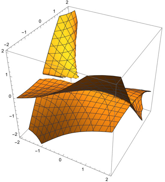
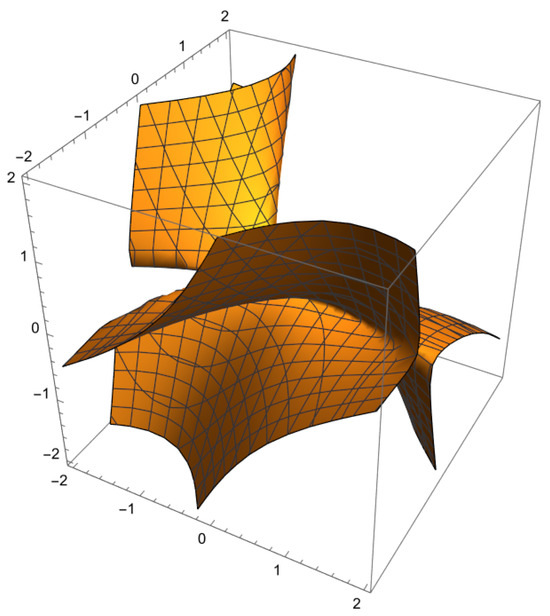
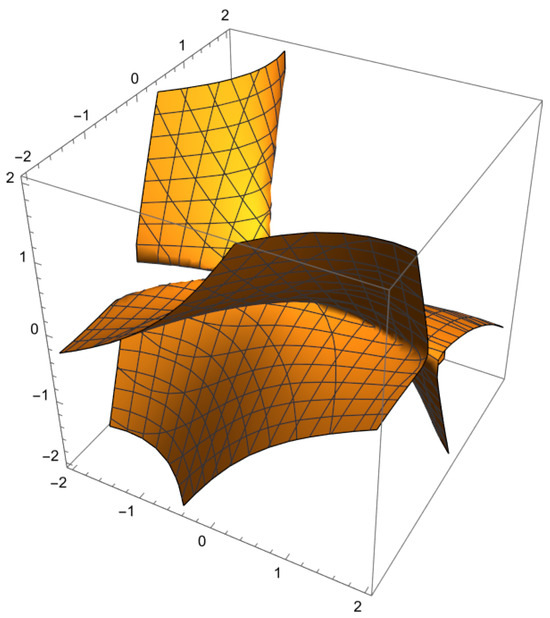
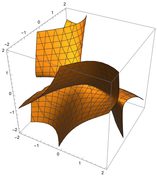
The graphs of ${\mathcal{Q}}_6\left({\lambda }_1,{\lambda }_2,{\lambda }_3;1.5\right)$, ${\mathcal{Q}}_6\left({\lambda }_1,{\lambda }_2,{\lambda }_3;2\right)$, ${\mathcal{Q}}_6\left({\lambda }_1,{\lambda }_2,{\lambda }_3;2.5\right)$ and ${\mathcal{Q}}_6\left({\lambda }_1,{\lambda }_2,{\lambda }_3;3\right)$ are expressed in Figure 1, Figure 2, Figure 3 and Figure 4, respectively as:

Operational techniques for special polynomials involve using specific algebraic and analytical methods to manipulate and apply these polynomials in various mathematical contexts. Techniques such as generating functions, which encode polynomial sequences into a single function, facilitate the derivation and proof of polynomial identities and relationships. Differential operators, another key method, express recurrence relations and transform polynomials to simplify solving differential equations. Additionally, integral transforms, such as the Laplace and Fourier transforms, help extend the applicability of special polynomials to solving physical problems in fields like quantum mechanics and signal processing. These operational techniques streamline complex calculations, making special polynomials powerful tools in pure and applied mathematics.

Differentiating (9) or (10) with reference to ${\lambda }_1$ successively, we find

$$\begin{array}{cc}\hfill {\displaystyle \frac{\partial }{\partial {\lambda }_1}}\left( {\mathcal{C}}^{{\lambda }_1\Omega +{\lambda }_2{\Omega }^2+{\lambda }_3{\Omega }^3}\right)& =\left(\ln \mathcal{C}\right)\Omega \left( {\mathcal{C}}^{{\lambda }_1\Omega +{\lambda }_2{\Omega }^2+{\lambda }_3{\Omega }^3}\right),\hfill \end{array}$$

which can be expressed further as

$${\displaystyle \frac{\partial }{\partial {\lambda }_1}}\left(\sum _{n=0}^{\infty } {\mathcal{Q}}_n({\lambda }_1,{\lambda }_2,{\lambda }_3;\mathcal{C}){\displaystyle \frac{{\Omega }^n}{n!}}\right)=\left(\ln \mathcal{C}\right)\left(\sum _{n=0}^{\infty } {\mathcal{Q}}_n({\lambda }_1,{\lambda }_2,{\lambda }_3;\mathcal{C}){\displaystyle \frac{{\Omega }^{n+1}}{n!}}\right),$$

replacing $n\to n-1$ in the right-hand side of the preceding expression and then comparing the coefficients of the same exponents on both sides of the resultant expression, we find

$${\displaystyle \frac{\partial }{\partial {\lambda }_1}}{\mathcal{Q}}_n({\lambda }_1,{\lambda }_2,{\lambda }_3;\mathcal{C})=n\ln \mathcal{C}{\mathcal{Q}}_{n-1}({\lambda }_1,{\lambda }_2,{\lambda }_3;\mathcal{C}).$$

(14)

Continuing similarly, we have

$${\displaystyle \frac{{\partial }^2}{\partial {\lambda }_1^2}}{\mathcal{Q}}_n({\lambda }_1,{\lambda }_2,{\lambda }_3;\mathcal{C})=n(n-1){\left(\ln \mathcal{C}\right)}^2{\mathcal{Q}}_{n-2}({\lambda }_1,{\lambda }_2,{\lambda }_3;\mathcal{C}),$$

(15)

$${\displaystyle \frac{{\partial }^3}{\partial {\lambda }_1^3}}{\mathcal{Q}}_n({\lambda }_1,{\lambda }_2,{\lambda }_3;\mathcal{C})=n(n-1)(n-2){\left(\ln \mathcal{C}\right)}^3{\mathcal{Q}}_{n-3}({\lambda }_1,{\lambda }_2,{\lambda }_3;\mathcal{C}),$$

(16)

$$⋮⋮$$

$${\displaystyle \frac{{\partial }^m}{\partial {\lambda }_1^m}}{\mathcal{Q}}_n({\lambda }_1,{\lambda }_2,{\lambda }_3;\mathcal{C})=n(n-1)\cdots (n-m+1){\left(\ln \mathcal{C}\right)}^m{\mathcal{Q}}_{n-m}({\lambda }_1,{\lambda }_2,{\lambda }_3;\mathcal{C}).$$

(17)

Further, differentiating (9) or (10) with reference to ${\lambda }_2$ successively, we find

$$\begin{array}{cc}\hfill {\displaystyle \frac{\partial }{\partial {\lambda }_2}}\left( {\mathcal{C}}^{{\lambda }_1\Omega +{\lambda }_2{\Omega }^2+{\lambda }_3{\Omega }^3}\right)& =\left(\ln \mathcal{C}\right){\Omega }^2\left( {\mathcal{C}}^{{\lambda }_1\Omega +{\lambda }_2{\Omega }^2+{\lambda }_3{\Omega }^3}\right),\hfill \end{array}$$

which further can be expressed as

$${\displaystyle \frac{\partial }{\partial {\lambda }_2}}\left(\sum _{n=0}^{\infty } {\mathcal{Q}}_n({\lambda }_1,{\lambda }_2,{\lambda }_3;\mathcal{C}){\displaystyle \frac{{\Omega }^n}{n!}}\right)=\left(\ln \mathcal{C}\right)\left(\sum _{n=0}^{\infty } {\mathcal{Q}}_n({\lambda }_1,{\lambda }_2,{\lambda }_3;\mathcal{C}){\displaystyle \frac{{\Omega }^{n+2}}{n!}}\right),$$

replacing $n\to n-2$ in the right-hand side of the preceding expression and then comparing the coefficients of the same exponents on both sides of the resultant expression, we find

$${\displaystyle \frac{\partial }{\partial {\lambda }_2}}{\mathcal{Q}}_n({\lambda }_1,{\lambda }_2,{\lambda }_3;\mathcal{C})=n(n-1)\ln \mathcal{C}{\mathcal{Q}}_{n-2}({\lambda }_1,{\lambda }_2,{\lambda }_3;\mathcal{C}),$$

(18)

similarly, we have

$${\displaystyle \frac{\partial }{\partial {\lambda }_3}}{\mathcal{Q}}_n({\lambda }_1,{\lambda }_2,{\lambda }_3;\mathcal{C})=n(n-1)(n-2)\ln \mathcal{C}{\mathcal{Q}}_{n-3}({\lambda }_1,{\lambda }_2,{\lambda }_3;\mathcal{C}).$$

(19)

Thus, the expressions (14)–(19) satisfy the relations:

$${\displaystyle \frac{1}{\ln \mathcal{C}}}{\displaystyle \frac{\partial }{\partial {\lambda }_2}}{\mathcal{Q}}_n({\lambda }_1,{\lambda }_2,{\lambda }_3;\mathcal{C})={\displaystyle \frac{{\partial }^2}{\partial {\lambda }_1^2}}{\mathcal{Q}}_n({\lambda }_1,{\lambda }_2,{\lambda }_3;\mathcal{C})$$

and

$${\displaystyle \frac{1}{{\left(\ln \mathcal{C}\right)}^2}}{\displaystyle \frac{\partial }{\partial {\lambda }_3}}{\mathcal{Q}}_n({\lambda }_1,{\lambda }_2,{\lambda }_3;\mathcal{C})={\displaystyle \frac{{\partial }^3}{\partial {\lambda }_1^3}}{\mathcal{Q}}_n({\lambda }_1,{\lambda }_2,{\lambda }_3;\mathcal{C}),$$

which in consideration of the initial condition:

$${\displaystyle \frac{1}{{\left(\ln \mathcal{C}\right)}^n}}{\mathcal{Q}}_n({\lambda }_1,0,0;0)={\lambda }_1^n$$

(20)

provides the operational representation for ${\mathcal{Q}}_n({\lambda }_1,{\lambda }_2,{\lambda }_3;\mathcal{C})$ via the result:

Theorem 3.

For the G-1P3-VHP ${\mathcal{Q}}_n({\lambda }_1,{\lambda }_2,{\lambda }_3;\mathcal{C})$, the following operational representation is demonstrated:

$${\mathcal{Q}}_n({\lambda }_1,{\lambda }_2,{\lambda }_3;\mathcal{C})=exp\left({\lambda }_2\left(\ln \mathcal{C}\right){\displaystyle \frac{{\partial }^2}{\partial {\lambda }_1^2}}+{\lambda }_3{\left(\ln \mathcal{C}\right)}^2{\displaystyle \frac{{\partial }^3}{\partial {\lambda }_1^3}}\right)\left\{{\lambda }_1^n\right\}.$$

(21)

3. Recurrence Relations, Shift Operators and Families of Differential Equations

Theorem 4.

The G-1P3-VHP ${\mathcal{Q}}_n({\lambda }_1,{\lambda }_2,{\lambda }_3;\mathcal{C})$ adhere to the following recurrence relation:

$$\begin{array}{cc} {\mathcal{Q}}_{n+1}({\lambda }_1,{\lambda }_2,{\lambda }_3;\mathcal{C})\hfill & =\left({\lambda }_1\ln \mathcal{C}\right) {\mathcal{Q}}_n({\lambda }_1,{\lambda }_2,{\lambda }_3;\mathcal{C})\hfill \\ \hfill & +2n{\lambda }_2\ln \mathcal{C} {\mathcal{Q}}_{n-2}({\lambda }_1,{\lambda }_2,{\lambda }_3;\mathcal{C})+3n(n-1){\lambda }_3\ln \mathcal{C} {\mathcal{Q}}_{n-2}({\lambda }_1,{\lambda }_2,{\lambda }_3;\mathcal{C}),\hfill \end{array}$$

(22)

where

$${\mathcal{Q}}_{-k}({\lambda }_1,{\lambda }_2,{\lambda }_3;\mathcal{C}):=0,k=1,2.$$

(23)

Proof. 

After taking $\Omega$ into account and differentiating both sides of the generating function (9), we arrive at:

$${\displaystyle \frac{\partial }{\partial \Omega }}\left\{ {\mathcal{C}}^{{\lambda }_1\Omega +{\lambda }_2{\Omega }^2+{\lambda }_3{\Omega }^3}\right\}={\displaystyle \frac{\partial }{\partial \Omega }}\left\{\sum _{n=0}^{\infty } {\mathcal{Q}}_n({\lambda }_1,{\lambda }_2,{\lambda }_3;\mathcal{C}){\displaystyle \frac{{\Omega }^n}{n!}}\right\}$$

(24)

which can be simplified as

$$\left\{{\lambda }_1\ln \left(\mathcal{C}\right)+2{\lambda }_2\ln \left(\mathcal{C}\right)\Omega +3{\lambda }_2\ln \left(\mathcal{C}\right){\Omega }^2\right\}\sum _{n=0}^{\infty } {\mathcal{Q}}_n({\lambda }_1,{\lambda }_2,{\lambda }_3;\mathcal{C}){\displaystyle \frac{{\Omega }^n}{n!}}=\sum _{n=0}^{\infty }n {\mathcal{Q}}_n({\lambda }_1,{\lambda }_2,{\lambda }_3;\mathcal{C}){\displaystyle \frac{{\Omega }^{n-1}}{n!}}.$$

Further, the preceding expression, in consideration of the Cauchy-product formula, can be expressed as:

$$\begin{array}{cc}\hfill \sum _{n=0}^{\infty }[{\lambda }_1\ln \left(\mathcal{C}\right) {\mathcal{Q}}_n({\lambda }_1,{\lambda }_2,{\lambda }_3;\mathcal{C})+2n{\lambda }_2\ln \left(\mathcal{C}\right) {\mathcal{Q}}_{n-1}({\lambda }_1,{\lambda }_2,{\lambda }_3;\mathcal{C})+3n(n-1){\lambda }_3\ln \left(\mathcal{C}\right)& \\ \hfill \times {\mathcal{Q}}_{n-2}({\lambda }_1,{\lambda }_2,{\lambda }_3;\mathcal{C})] {\mathcal{Q}}_n({\lambda }_1,{\lambda }_2,{\lambda }_3;\mathcal{C}){\displaystyle \frac{{\Omega }^n}{n!}}=\sum _{n=0}^{\infty } {\mathcal{Q}}_{n+1}({\lambda }_1,{\lambda }_2,{\lambda }_3;\mathcal{C}){\displaystyle \frac{{\Omega }^n}{n!}}.\end{array}$$

(25)

Assertion (22) is obtained by comparing the coefficients of the identical powers of $\Omega$ on both sides of the preceding statement. □

Theorem 5.

For, the G-1P3-VHP ${\mathcal{Q}}_n({\lambda }_1,{\lambda }_2,{\lambda }_3;\mathcal{C})$, the following shift operators hold true:

$${\lambda }_1{\mathcal{L}}_n^{-}:={\displaystyle \frac{1}{n\left(\ln \mathcal{C}\right)}}{D}_{{\lambda }_1},$$

(26)

$${\lambda }_2{\mathcal{L}}_n^{-}:={\displaystyle \frac{1}{n\left(\ln \mathcal{C}\right)}}{D}_{{\lambda }_1}^{-1}{D}_{{\lambda }_2},$$

(27)

$${\lambda }_3{\mathcal{L}}_n^{-}:={\displaystyle \frac{1}{n\left(\ln \mathcal{C}\right)}}{D}_{{\lambda }_1}^{-2}{D}_{{\lambda }_3},$$

(28)

$${\lambda }_1{\mathcal{L}}_n^{+}:=\left({\lambda }_1\ln \mathcal{C}\right)+2{\lambda }_2{D}_{{\lambda }_1}+3{\lambda }_3{\left(\ln \mathcal{C}\right)}^{-1}{D}_{{\lambda }_1}^2,$$

(29)

$${\lambda }_2{\mathcal{L}}_n^{+}:=\left({\lambda }_1\ln \mathcal{C}\right)+2{\lambda }_2{D}_{{\lambda }_1}^{-1}{D}_{{\lambda }_2}+3{\lambda }_3{\left(\ln \mathcal{C}\right)}^{-1}{D}_{{\lambda }_1}^{-2}{D}_{{\lambda }_2}^2$$

(30)

and

$${\lambda }_3{\mathcal{L}}_n^{+}:=\left({\lambda }_1\ln \mathcal{C}\right)+2{\lambda }_2{D}_{{\lambda }_1}^{-1}{D}_{{\lambda }_3}+3{\lambda }_3{\left(\ln \mathcal{C}\right)}^{-1}{D}_{{\lambda }_1}^{-4}{D}_{{\lambda }_3}^2$$

(31)

respectively, where

$$D_{{\lambda }_1}:={\displaystyle \frac{\partial }{{\partial }_{{\lambda }_1}}},D_{{\lambda }_2}:={\displaystyle \frac{\partial }{{\partial }_{{\lambda }_2}}};D_{{\lambda }_3}:={\displaystyle \frac{\partial }{{\partial }_{{\lambda }_3}}}{D}_{{\lambda }_1}^{-1}:=\underset{0}{\overset{{\lambda }_1}{\int }}g(\Omega )d\Omega .$$

(32)

Proof. 

After rearranging the powers and differentiating both sides of Equation (9) concerning ${\lambda }_1$, we equate the coefficients of the identical powers of $\Omega$ in both sides of the resulting equation as follows:

$$D_{{\lambda }_1}\left\{ {\mathcal{Q}}_n({\lambda }_1,{\lambda }_2,{\lambda }_3;\mathcal{C})\right\}=n\left(\ln \mathcal{C}\right) {\mathcal{Q}}_{n-1}({\lambda }_1,{\lambda }_2,{\lambda }_3;\mathcal{C}),$$

(33)

as a result, the operator provided by Equation (26) satisfies the following equation:

$${\lambda }_1{\mathcal{L}}_n^{-}\left\{{\mathcal{Q}}_n({\lambda }_1,{\lambda }_2,{\lambda }_3;\mathcal{C})\right\}= {\mathcal{Q}}_{n-1}({\lambda }_1,{\lambda }_2,{\lambda }_3;\mathcal{C}).$$

(34)

Subsequently, we differentiate both sides of Equation (9) concerning ${\lambda }_2$, rearrange the powers, and then calculate the coefficients of the identical powers of $\Omega$ on both sides of the resulting equation:

$$D_{{\lambda }_2}\left\{ {\mathcal{Q}}_n({\lambda }_1,{\lambda }_2,{\lambda }_3;\mathcal{C})\right\}=\left(\ln \mathcal{C}\right)n(n-1) {\mathcal{Q}}_{n-2}({\lambda }_1,{\lambda }_2,{\lambda }_3;\mathcal{C}),$$

(35)

which further can be stated as

$$D_{{\lambda }_2}\left\{ {\mathcal{Q}}_n({\lambda }_1,{\lambda }_2,{\lambda }_3;\mathcal{C})\right\}=n\left(\ln \mathcal{C}\right)D_{{\lambda }_1} {\mathcal{Q}}_{n-1}({\lambda }_1,{\lambda }_2,{\lambda }_3;\mathcal{C}),$$

(36)

thus, it follows that

$${\displaystyle \frac{1}{n\left(\ln \mathcal{C}\right)}}{D}_{{\lambda }_2}{D}_{{\lambda }_1}^{-1}\left\{ {\mathcal{Q}}_n({\lambda }_1,{\lambda }_2,{\lambda }_3;\mathcal{C})\right\}= {\mathcal{Q}}_{n-1}({\lambda }_1,{\lambda }_2,{\lambda }_3;\mathcal{C}).$$

(37)

Thus, the above equation is satisfied by the operator provided by Equation (27).

Again, differentiating both sides of Equation (9) with respect to ${\lambda }_3$, we have

$$D_{{\lambda }_3}\left\{ {\mathcal{Q}}_n({\lambda }_1,{\lambda }_2,{\lambda }_3;\mathcal{C})\right\}=\left(\ln \mathcal{C}\right)n(n-1)(n-2) {\mathcal{Q}}_{n-3}({\lambda }_1,{\lambda }_2,{\lambda }_3;\mathcal{C})$$

(38)

and further stated as

$$D_{{\lambda }_3}\left\{ {\mathcal{Q}}_n({\lambda }_1,{\lambda }_2,{\lambda }_3;\mathcal{C})\right\}=n\left(\ln \mathcal{C}\right)D_{{\lambda }_1}^2 {\mathcal{Q}}_{n-1}({\lambda }_1,{\lambda }_2,{\lambda }_3;\mathcal{C}),$$

(39)

thus, it follows that

$${\displaystyle \frac{1}{n\left(\ln \mathcal{C}\right)}}{D}_{{\lambda }_3}{D}_{{\lambda }_1}^{-2}\left\{ {\mathcal{Q}}_n({\lambda }_1,{\lambda }_2,{\lambda }_3;\mathcal{C})\right\}= {\mathcal{Q}}_{n-1}({\lambda }_1,{\lambda }_2,{\lambda }_3;\mathcal{C}).$$

(40)

Thus, the above equation is satisfied by the operator provided by Equation (28).

The raising operator (29) may be found using the following relation:

$${\mathcal{Q}}_{n-k}({\lambda }_1,{\lambda }_2,{\lambda }_3;\mathcal{C})=\left({\lambda }_1{\mathcal{L}}_{n-k+1}^{-}{\lambda }_1{\mathcal{L}}_{n-k+2}^{-}\cdots {\lambda }_1{\mathcal{L}}_{n-1}^{-}{\lambda }_1{\mathcal{L}}_n^{-}\right)\left\{ {\mathcal{Q}}_n({\lambda }_1,{\lambda }_2,{\lambda }_3;\mathcal{C})\right\}.$$

(41)

Using Equation (26) in conjunction with Equation (41), we obtain

$${\mathcal{Q}}_{n-k}({\lambda }_1,{\lambda }_2,{\lambda }_3;\mathcal{C})=\left({\displaystyle \frac{1}{(n-k+1)\left(\ln \mathcal{C}\right)}}{D}_{{\lambda }_1}\cdots {\displaystyle \frac{1}{(n-1)\left(\ln \mathcal{C}\right)}}{D}_{{\lambda }_1}{\displaystyle \frac{1}{n\left(\ln \mathcal{C}\right)}}{D}_{{\lambda }_1}\right)\left\{ {\mathcal{Q}}_n({\lambda }_1,{\lambda }_2,{\lambda }_3;\mathcal{C})\right\}$$

(42)

and further stated as

$${\mathcal{Q}}_{n-k}({\lambda }_1,{\lambda }_2,{\lambda }_3;\mathcal{C})={\displaystyle \frac{(n-k)!}{n!}}{\left(\ln \mathcal{C}\right)}^{-k}{D}_{{\lambda }_1}^k\left\{{\mathcal{Q}}_n({\lambda }_1,{\lambda }_2,{\lambda }_3;\mathcal{C})\right\}.$$

(43)

Further, we have

$${\mathcal{Q}}_{n-1}({\lambda }_1,{\lambda }_2,{\lambda }_3;\mathcal{C})={\displaystyle \frac{1}{n}}{\left(\ln \mathcal{C}\right)}^{-1}{D}_{{\lambda }_1}\left\{{\mathcal{Q}}_n({\lambda }_1,{\lambda }_2,{\lambda }_3;\mathcal{C})\right\}.$$

(44)

Thus, inserting expressions (41) and (43) in Equation (22), we find

$$\begin{array}{cc}\hfill {\mathcal{Q}}_{n+1}({\lambda }_1,{\lambda }_2,{\lambda }_3;\mathcal{C})& =\left(\left({\lambda }_1\ln \mathcal{C}\right)+2{\lambda }_2{D}_{{\lambda }_1}^{-1}{D}_{{\lambda }_2}+3{\lambda }_3{\left(\ln \mathcal{C}\right)}^{-1}{D}_{{\lambda }_1}^{-2}{D}_{{\lambda }_2}^2\right)\left\{ {\mathcal{Q}}_n({\lambda }_1,{\lambda }_2,{\lambda }_3;\mathcal{C})\right\},\hfill \end{array}$$

thus yielding the expression (29) of the raising operator ${\lambda }_3{\mathcal{L}}_n^{+}$.

We employ the relation below to determine the raising operator (30):

$${\mathcal{Q}}_{n-k}({\lambda }_1,{\lambda }_2,{\lambda }_3;\mathcal{C})=\left({\lambda }_2{\mathcal{L}}_{n-k+1}^{-}{\lambda }_2{\mathcal{L}}_{n-k+2}^{-}\cdots {\lambda }_2{\mathcal{L}}_{n-1}^{-}{\lambda }_2{\mathcal{L}}_n^{-}\right)\left\{ {\mathcal{Q}}_n({\lambda }_1,{\lambda }_2,{\lambda }_3;\mathcal{C})\right\}$$

(45)

Using Equation (27) in Equation (45) and simplifying, we find

$${\mathcal{Q}}_{n-k}({\lambda }_1,{\lambda }_2,{\lambda }_3;\mathcal{C})={\displaystyle \frac{(n-k)!}{n!}}{\left(\ln \mathcal{C}\right)}^{-k}{D}_{{\lambda }_1}^{-k}{D}_{{\lambda }_2}^k\left\{ {\mathcal{Q}}_n({\lambda }_1,{\lambda }_2,{\lambda }_3;\mathcal{C})\right\}.$$

(46)

Also, we have

$${\mathcal{Q}}_{n-1}({\lambda }_1,{\lambda }_2,{\lambda }_3;\mathcal{C})={\displaystyle \frac{1}{n}}{\left(\ln \mathcal{C}\right)}^{-1}{D}_{{\lambda }_1}^{-1}{D}_{{\lambda }_2}\left\{ {\mathcal{Q}}_n({\lambda }_1,{\lambda }_2,{\lambda }_3;\mathcal{C})\right\}.$$

(47)

Using Equations (46) and (47) in Equation (22), we find

$$\begin{array}{cc} {\mathcal{Q}}_{n+1}({\lambda }_1,{\lambda }_2,{\lambda }_3;\mathcal{C})=\hfill & \left(\left({\lambda }_1\ln \mathcal{C}\right)+2{\lambda }_2{D}_{{\lambda }_1}^{-1}{D}_{{\lambda }_2}+3{\lambda }_3{\left(\ln \mathcal{C}\right)}^{-1}{D}_{{\lambda }_1}^{-2}{D}_{{\lambda }_2}^2\right) {\mathcal{Q}}_n({\lambda }_1,{\lambda }_2,{\lambda }_3;\mathcal{C}),\hfill \end{array}$$

(48)

thus yielding the expression (30) of the raising operator ${\lambda }_3{\mathcal{L}}_n^{+}$.

Lastly, we employ the relation below to determine the raising operator (31):

$${\mathcal{Q}}_{n-k}({\lambda }_1,{\lambda }_2,{\lambda }_3;\mathcal{C})=\left({\lambda }_3{\mathcal{L}}_{n-k+1}^{-}{\lambda }_3{\mathcal{L}}_{n-k+2}^{-}\cdots {\lambda }_3{\mathcal{L}}_{n-1}^{-}{\lambda }_3{\mathcal{L}}_n^{-}\right)\left\{ {\mathcal{Q}}_n({\lambda }_1,{\lambda }_2,{\lambda }_3;\mathcal{C})\right\}$$

(49)

Using Equation (28) in Equation (49) and simplifying, we find

$${\mathcal{Q}}_{n-k}({\lambda }_1,{\lambda }_2,{\lambda }_3;\mathcal{C})={\displaystyle \frac{(n-k)!}{n!}}{\left(\ln \mathcal{C}\right)}^{-k}{D}_{{\lambda }_1}^{-2k}{D}_{{\lambda }_2}^k\left\{ {\mathcal{Q}}_n({\lambda }_1,{\lambda }_2,{\lambda }_3;\mathcal{C})\right\}.$$

(50)

Also, we have

$${\mathcal{Q}}_{n-1}({\lambda }_1,{\lambda }_2,{\lambda }_3;\mathcal{C})={\displaystyle \frac{1}{n}}{\left(\ln \mathcal{C}\right)}^{-1}{D}_{{\lambda }_1}^{-2}{D}_{{\lambda }_3}\left\{ {\mathcal{Q}}_n({\lambda }_1,{\lambda }_2,{\lambda }_3;\mathcal{C})\right\}.$$

(51)

Using Equations (50) and (51) in Equation (22), we find

$$\begin{array}{cc} {\mathcal{Q}}_{n+1}({\lambda }_1,{\lambda }_2,{\lambda }_3;\mathcal{C})=\hfill & \left(\left({\lambda }_1\ln \mathcal{C}\right)+2{\lambda }_2{D}_{{\lambda }_1}^{-1}{D}_{{\lambda }_3}+3{\lambda }_3{\left(\ln \mathcal{C}\right)}^{-1}{D}_{{\lambda }_1}^{-4}{D}_{{\lambda }_3}^2\right) {\mathcal{Q}}_n({\lambda }_1,{\lambda }_2,{\lambda }_3;\mathcal{C}),\hfill \end{array}$$

(52)

thus yielding the expression (31) of the raising operator ${\lambda }_3{\mathcal{L}}_n^{+}$. □

Next, we find the “differential, integro-differential and partial differential equation” for the 3V1PGHbAP ${\mathcal{Q}}_n({\lambda }_1,{\lambda }_2,{\lambda }_3;\mathcal{C})$. For this, we consider the following results:

Theorem 6.

The generalized 1-parameter 3-variable Hermite polynomials ${\mathcal{Q}}_n({\lambda }_1,{\lambda }_2,{\lambda }_3;\mathcal{C})$ satisfy the following differential equation:

$$\left({\lambda }_1{D}_{{\lambda }_1}+2{\lambda }_2{\left(\ln \mathcal{C}\right)}^{-1}{D}_{{\lambda }_1}^2+3{\lambda }_3{\left(\ln \mathcal{C}\right)}^{-2}{D}_{{\lambda }_1}^3-(n+1)\right) {\mathcal{Q}}_n({\lambda }_1,{\lambda }_2,{\lambda }_3;\mathcal{C})=0.$$

(53)

Proof. 

Making use of expressions (26) and (28) of the shift operators ${\lambda }_1{\mathcal{L}}_n^{-}$ and ${\lambda }_1{\mathcal{L}}_n^{+}$ in the factorization equation ${\lambda }_1{\mathcal{L}}_{n+1}^{-}{\lambda }_1{\mathcal{L}}_n^{+}\left\{ {\mathcal{Q}}_n({\lambda }_1,{\lambda }_2,{\lambda }_3;\mathcal{C})\right\}= {\mathcal{Q}}_n({\lambda }_1,{\lambda }_2,{\lambda }_3;\mathcal{C})$, we adhere to the expression (53). □

Theorem 7.

The generalized 1-parameter 3-variable Hermite polynomials ${\mathcal{Q}}_n({\lambda }_1,{\lambda }_2,{\lambda }_3;\mathcal{C})$ satisfy the following integro-differential equations:

$$\begin{array}{c}\hfill \left({\lambda }_1{D}_{{\lambda }_2}+2{\lambda }_2{\left(\ln \mathcal{C}\right)}^{-1}{D}_{{\lambda }_1}^{-1}{D}_{{\lambda }_2}^2+3{\lambda }_3{\left(\ln \mathcal{C}\right)}^{-2}{D}_{{\lambda }_1}^{-2}{D}_{{\lambda }_2}^3-(n+1)D_{{\lambda }_1}\right) {\mathcal{Q}}_n({\lambda }_1,{\lambda }_2,{\lambda }_3;\mathcal{C})=0.\end{array}$$

(54)

$$\begin{array}{c}\hfill \left({\lambda }_1{D}_{{\lambda }_3}+2{\lambda }_2{\left(\ln \mathcal{C}\right)}^{-1}{D}_{{\lambda }_1}^{-1}{D}_{{\lambda }_3}^2+3{\lambda }_3{\left(\ln \mathcal{C}\right)}^{-2}{D}_{{\lambda }_1}^{-4}{D}_{{\lambda }_3}^3-(n+1)D_{{\lambda }_1}^2\right) {\mathcal{Q}}_n({\lambda }_1,{\lambda }_2,{\lambda }_3;\mathcal{C})=0.\end{array}$$

(55)

$$\begin{array}{c}\hfill \left({\lambda }_1{D}_{{\lambda }_3}+2{\lambda }_2{\left(\ln \mathcal{C}\right)}^{-1}{D}_{{\lambda }_1}^{-1}{D}_{{\lambda }_2}^2{D}_{{\lambda }_3}+3{\lambda }_3{\left(\ln \mathcal{C}\right)}^{-2}{D}_{{\lambda }_1}^{-2}{D}_{{\lambda }_2}^3{D}_{{\lambda }_3}-(n+1)D_{{\lambda }_1}^2\right) {\mathcal{Q}}_n({\lambda }_1,{\lambda }_2,{\lambda }_3;\mathcal{C})=0.\end{array}$$

(56)

$$\begin{array}{c}\hfill \left({\lambda }_1{D}_{{\lambda }_2}+2{\lambda }_2{\left(\ln \mathcal{C}\right)}^{-1}{D}_{{\lambda }_1}^{-1}{D}_{{\lambda }_2}{D}_{{\lambda }_3}+3{\lambda }_3{\left(\ln \mathcal{C}\right)}^{-2}{D}_{{\lambda }_1}^{-4}{D}_{{\lambda }_2}{D}_{{\lambda }_3}^2-(n+1)D_{{\lambda }_1}\right) {\mathcal{Q}}_n({\lambda }_1,{\lambda }_2,{\lambda }_3;\mathcal{C})=0.\end{array}$$

(57)

Proof. 

Making use of expressions (27), (30) and (28), (31) of the shift operators ${\mathcal{L}}_n^{-}$ and ${\mathcal{L}}_n^{+}$ in the factorization equation ${\mathcal{L}}_{n+1}^{-} {\mathcal{L}}_n^{+}\left\{ {\mathcal{Q}}_n({\lambda }_1,{\lambda }_2,{\lambda }_3;\mathcal{C})\right\}= {\mathcal{Q}}_n({\lambda }_1,{\lambda }_2,{\lambda }_3;\mathcal{C})$, we adhere to the expression (54) and (55).

Further, making use of expressions (27), (31) and (28), (30) of the shift operators ${\mathcal{L}}_n^{-}$ and ${\mathcal{L}}_n^{+}$ in above factorization relation, we adhere to the expression (56) and (57). □

Theorem 8.

The generalized 1-parameter 3-variable Hermite polynomials ${\mathcal{Q}}_n({\lambda }_1,{\lambda }_2,{\lambda }_3;\mathcal{C})$ satisfy the following partial differential equations:

$$\begin{array}{c}({\lambda }_1{D}_{{\lambda }_1}^n{D}_{{\lambda }_2}+n{D}_{{\lambda }_1}^{n-1}{D}_{{\lambda }_2}+2{\lambda }_2{\left(\ln \mathcal{C}\right)}^{-1}{D}_{{\lambda }_1}^{n-1}{D}_{{\lambda }_2}^2+2{\left(\ln \mathcal{C}\right)}^{-1}{D}_{{\lambda }_1}^{n-1}{D}_{{\lambda }_2}+3{\lambda }_3{\left(\ln \mathcal{C}\right)}^{-2}{D}_{{\lambda }_1}^{n-2}{D}_{{\lambda }_2}^3\hfill \\ \hfill -(n+1)D_{{\lambda }_1}^{n+1}) {\mathcal{Q}}_n({\lambda }_1,{\lambda }_2,{\lambda }_3;\mathcal{C})=0.\end{array}$$

(58)

$$\begin{array}{c}({\lambda }_1{D}_{{\lambda }_1}^{2n}{D}_{{\lambda }_3}+2n{D}_{{\lambda }_1}^{2n-1}{D}_{{\lambda }_3}+2{\lambda }_2{\left(\ln \mathcal{C}\right)}^{-1}{D}_{{\lambda }_1}^{-1}{D}_{{\lambda }_3}^2+3{\lambda }_3{\left(\ln \mathcal{C}\right)}^{-2}{D}_{{\lambda }_1}^{2n-4}{D}_{{\lambda }_3}^3+3{\left(\ln \mathcal{C}\right)}^{-2}{D}_{{\lambda }_1}^{2n-4}{D}_{{\lambda }_3}^2\hfill \\ \hfill -(n+1)D_{{\lambda }_1}^{2n+2}) {\mathcal{Q}}_n({\lambda }_1,{\lambda }_2,{\lambda }_3;\mathcal{C})=0.\end{array}$$

(59)

$$\begin{array}{c}({\lambda }_1{D}_{{\lambda }_1}^n{D}_{{\lambda }_3}+n{D}_{{\lambda }_1}^{n-1}{D}_{{\lambda }_3}+2{\lambda }_2{\left(\ln \mathcal{C}\right)}^{-1}{D}_{{\lambda }_1}^{n-1}{D}_{{\lambda }_2}^2{D}_{{\lambda }_3}+3{\left(\ln \mathcal{C}\right)}^{-2}{D}_{{\lambda }_1}^{n-2}{D}_{{\lambda }_2}^2+3{\lambda }_3{\left(\ln \mathcal{C}\right)}^{-2}{D}_{{\lambda }_1}^{n-2}{D}_{{\lambda }_2}^3{D}_{{\lambda }_3}\hfill \\ \hfill -(n+1)D_{{\lambda }_1}^{n+2}) {\mathcal{Q}}_n({\lambda }_1,{\lambda }_2,{\lambda }_3;\mathcal{C})=0.\end{array}$$

(60)

$$\begin{array}{c}({\lambda }_1{D}_{{\lambda }_1}^{2n}{D}_{{\lambda }_2}+2n{D}_{{\lambda }_1}^{2n-1}{D}_{{\lambda }_2}+2{\left(\ln \mathcal{C}\right)}^{-1}{D}_{{\lambda }_1}^{2n-1}{D}_{{\lambda }_3}+2{\lambda }_2{\left(\ln \mathcal{C}\right)}^{-1}{D}_{{\lambda }_1}^{2n-1}{D}_{{\lambda }_2}{D}_{{\lambda }_3}+3{\lambda }_3{\left(\ln \mathcal{C}\right)}^{-2}{D}_{{\lambda }_1}^{2n-4}{D}_{{\lambda }_2}{D}_{{\lambda }_3}^2\hfill \\ \hfill -(n+1)D_{{\lambda }_1}^{2n}) {\mathcal{Q}}_n({\lambda }_1,{\lambda }_2,{\lambda }_3;\mathcal{C})=0.\end{array}$$

(61)

Proof. 

Differentiating the expressions (54) and (56) with reference to $D_{{\lambda }_1}$n times, we obtain the partial differential Equations (58) and (60). Similarly, upon differentiating the expressions (55) and (57) with reference to $D_{{\lambda }_1}$$2n$ times, we obtain the partial differential Equations (59) and (61). □

4. Summation Formulae

Summation formulae are vital tools in mathematics, significantly impacting fields like probability theory, combinatorics, and algebra. They enable the calculating of expected values in probabilistic models, aid in polynomial interpolation, and simplify combinatorial counting problems. These formulae are also crucial in number theory for analyzing arithmetic functions and in applied mathematics, such as in signal processing and optimization. By providing efficient methods to sum sequences and series, summation formulae for generalized 1-parameter 3-variable Hermite polynomials may facilitate the resolution of complex mathematical problems across diverse domains. Therefore, the summation formulae for the generalized 1-parameter 3-variable Hermite polynomials are demonstrated as follows:

Theorem 9.

For the G-1P3-VHP ${\mathcal{Q}}_n({\lambda }_1,{\lambda }_2,{\lambda }_3;\mathcal{C})$, the following summation formulae holds true:

$${\mathcal{Q}}_n({\lambda }_1+\mu ,{\lambda }_2,{\lambda }_3;\mathcal{C})=\sum _{k=0}^n\left({\displaystyle \genfrac{}{}{0pt}{}{n}{k}}\right) {\mathcal{Q}}_{n-k}({\lambda }_1,{\lambda }_2,{\lambda }_3;\mathcal{C}){\mathbb{R}}_k(\mu ,\mathcal{C}).$$

(62)

Proof. 

By substituting ${\lambda }_1\to {\lambda }_1+\mu$ in expression (9), it follows that

$${\mathcal{C}}^{({\lambda }_1+\mu )\Omega +{\lambda }_2{\Omega }^2+{\lambda }_3{\Omega }^3}=\sum _{n=0}^{\infty } {\mathcal{Q}}_n({\lambda }_1+\mu ,{\lambda }_2,{\lambda }_3;\mathcal{C}){\displaystyle \frac{{\Omega }^n}{n!}},\mathcal{C}>1,$$

(63)

Inserting expressions (4) and (9) in the left-hand part of preceding expression, we find

$$\sum _{n=0}^{\infty }{\mathcal{Q}}_n({\lambda }_1,{\lambda }_2,{\lambda }_3;\mathcal{C}){\displaystyle \frac{{\Omega }^n}{n!}}\sum _{k=0}^{\infty }{\mathbb{R}}_k(\mu ,\mathcal{C}){\displaystyle \frac{{\Omega }^k}{k!}}=\sum _{n=0}^{\infty } {\mathcal{Q}}_n({\lambda }_1+\mu ,{\lambda }_2,{\lambda }_3;\mathcal{C}){\displaystyle \frac{{\Omega }^n}{n!}},\mathcal{C}>1,$$

(64)

thus, operating the Cauchy-product rule in the left-hand part, yields the expression:

$$\sum _{n=0}^{\infty } {\mathcal{Q}}_n({\lambda }_1+\mu ,{\lambda }_2,{\lambda }_3;\mathcal{C}){\displaystyle \frac{{\Omega }^n}{n!}}=\sum _{n=0}^{\infty }\sum _{k=0}^n\left({\displaystyle \genfrac{}{}{0pt}{}{n}{k}}\right) {\mathcal{Q}}_{n-k}({\lambda }_1,{\lambda }_2,{\lambda }_3;\mathcal{C}){\mathbb{R}}_k(\mu ,\mathcal{C}){\displaystyle \frac{{\Omega }^n}{n!}}.$$

(65)

Assertion (62) is obtained by comparing the coefficients of the identical powers of $\Omega$ on both sides of the above expression. □

Theorem 10.

For the G-1P3-VHP ${\mathcal{Q}}_n({\lambda }_1,{\lambda }_2,{\lambda }_3;\mathcal{C})$, the following summation formulae holds true:

$${\mathcal{Q}}_n({\lambda }_1+\mu ,{\lambda }_2+\nu ,{\lambda }_3;\mathcal{C})=\sum _{k=0}^n\left({\displaystyle \genfrac{}{}{0pt}{}{n}{k}}\right) {\mathcal{Q}}_{n-k}({\lambda }_1,{\lambda }_2,{\lambda }_3;\mathcal{C}){\mathbb{R}}_k(\mu ,\nu ,\mathcal{C}).$$

(66)

Proof. 

By substituting ${\lambda }_1\to {\lambda }_1+\mu$ and ${\lambda }_{2}1\to {\lambda }_2+\nu$ in expression (9), it follows that

$${\mathcal{C}}^{({\lambda }_1+\mu )\Omega +({\lambda }_2+\nu ){\Omega }^2+{\lambda }_3{\Omega }^3}=\sum _{n=0}^{\infty } {\mathcal{Q}}_n({\lambda }_1+\mu ,{\lambda }_2+\nu ,{\lambda }_3;\mathcal{C}){\displaystyle \frac{{\Omega }^n}{n!}},\mathcal{C}>1,$$

(67)

Inserting expressions (3) and (9) in the left hand part of preceding expression, we find

$$\sum _{n=0}^{\infty }{\mathcal{Q}}_n({\lambda }_1,{\lambda }_2,{\lambda }_3;\mathcal{C}){\displaystyle \frac{{\Omega }^n}{n!}}\sum _{k=0}^{\infty }{\mathbb{R}}_k(\mu ,\nu ,\mathcal{C}){\displaystyle \frac{{\Omega }^k}{k!}}=\sum _{n=0}^{\infty } {\mathcal{Q}}_n({\lambda }_1+\mu ,{\lambda }_2+\nu ,{\lambda }_3;\mathcal{C}){\displaystyle \frac{{\Omega }^n}{n!}},\mathcal{C}>1,$$

(68)

thus, operating the Cauchy-product rule in the left-hand part yields the expression:

$$\sum _{n=0}^{\infty } {\mathcal{Q}}_n({\lambda }_1+\mu ,{\lambda }_2+\nu ,{\lambda }_3;\mathcal{C}){\displaystyle \frac{{\Omega }^n}{n!}}=\sum _{n=0}^{\infty }\sum _{k=0}^n\left({\displaystyle \genfrac{}{}{0pt}{}{n}{k}}\right) {\mathcal{Q}}_{n-k}({\lambda }_1,{\lambda }_2,{\lambda }_3;\mathcal{C}){\mathbb{R}}_k(\mu ,\nu ,\mathcal{C}){\displaystyle \frac{{\Omega }^n}{n!}}.$$

(69)

Assertion (66) is obtained by comparing the coefficients of the identical powers of $\Omega$ on both sides of the above expression. □

Theorem 11.

For the G-1P3-VHP ${\mathcal{Q}}_n({\lambda }_1,{\lambda }_2,{\lambda }_3;\mathcal{C})$, the following summation formulae holds true:

$${\mathcal{Q}}_n({\lambda }_1+\mu ,{\lambda }_2+\nu ,{\lambda }_3+\eta ;\mathcal{C})=\sum _{k=0}^n\left({\displaystyle \genfrac{}{}{0pt}{}{n}{k}}\right) {\mathcal{Q}}_{n-k}({\lambda }_1,{\lambda }_2,{\lambda }_3;\mathcal{C}){\mathbb{R}}_k(\mu ,\nu ,\eta ,\mathcal{C}).$$

(70)

Proof. 

By substituting ${\lambda }_1\to {\lambda }_1+\mu$, ${\lambda }_2\to {\lambda }_2+\nu$ and ${\lambda }_3\to {\lambda }_3+\eta$ in expression (9), it follows that

$${\mathcal{C}}^{({\lambda }_1+\mu )\Omega +({\lambda }_2+\nu ){\Omega }^2+({\lambda }_3+\eta ){\Omega }^3}=\sum _{n=0}^{\infty } {\mathcal{Q}}_n({\lambda }_1+\mu ,{\lambda }_2+\nu ,{\lambda }_3+\eta ;\mathcal{C}){\displaystyle \frac{{\Omega }^n}{n!}},\mathcal{C}>1,$$

(71)

Inserting expression (9) in the left hand part of preceding expression, we find

$$\sum _{n=0}^{\infty }{\mathcal{Q}}_n({\lambda }_1,{\lambda }_2,{\lambda }_3;\mathcal{C}){\displaystyle \frac{{\Omega }^n}{n!}}\sum _{k=0}^{\infty }{\mathbb{R}}_k(\mu ,\nu ,\eta ,\mathcal{C}){\displaystyle \frac{{\Omega }^k}{k!}}=\sum _{n=0}^{\infty } {\mathcal{Q}}_n({\lambda }_1+\mu ,{\lambda }_2+\nu ,{\lambda }_3+\eta ;\mathcal{C}){\displaystyle \frac{{\Omega }^n}{n!}},\mathcal{C}>1,$$

(72)

thus, operating the Cauchy-product rule in the left hand part yields the expression:

$$\sum _{n=0}^{\infty } {\mathcal{Q}}_n({\lambda }_1+\mu ,{\lambda }_2+\nu ,{\lambda }_3+\eta ;\mathcal{C}){\displaystyle \frac{{\Omega }^n}{n!}}=\sum _{n=0}^{\infty }\sum _{k=0}^n\left({\displaystyle \genfrac{}{}{0pt}{}{n}{k}}\right) {\mathcal{Q}}_{n-k}({\lambda }_1,{\lambda }_2,{\lambda }_3;\mathcal{C}){\mathbb{R}}_k(\mu ,\nu ,\eta ,\mathcal{C}){\displaystyle \frac{{\Omega }^n}{n!}}.$$

(73)

Assertion (70) is obtained by comparing the coefficients of the identical powers of $\Omega$ on both sides of the above expression. □

5. Conclusions

Here, we presented a novel framework for introducing generalized 1-parameter 3-variable Hermite polynomials. The essential characteristics of these polynomials are explained, utilizing generating functions and series definitions. This research uses a factorization technique to build recurrence relations, shift operators, and several differential equations, such as integro-differential, partial, and differential.

Further, future research could focus on extending the current framework to include more than three variables, exploring the associated complexities and new properties. Further examination of additional analytical properties, such as orthogonality, asymptotic behaviour, and zeros, is also warranted. Developing efficient computational algorithms to facilitate the practical application of these polynomials in various fields, such as numerical analysis, physics, and engineering, will be beneficial. Additionally, investigating their application in solving higher-order and more complex differential equations, particularly in modelling real-world phenomena, could yield significant insights. Interdisciplinary applications in finance, biology, and data science and enhanced graphical and numerical analyses could provide deeper insights and lead to new theoretical advancements.

References

- Dattoli, G.; Chiccoli, C.; Lorenzutta, S.; Maino, G.; Torre, A. Generalized Bessel functions and generalized Hermite polynomials. J. Math. Anal. Appl. 1993, 178, 509–516. [Google Scholar] [CrossRef]
- Dattoli, G.; Lorenzutta, S.; Maino, G.; Torre, A.; Cesarano, C. Generalized Hermite polynomials and super-Gaussian forms. J. Math. Anal. Appl. 1996, 203, 597–609. [Google Scholar] [CrossRef]
- Fadel, M.; Raza, N.; Du, W.-S. On q-Hermite Polynomials with Three Variables: Recurrence Relations, q-Differential Equations, Summation and Operational Formulas. Symmetry 2024, 16, 385. [Google Scholar] [CrossRef]
- Appell, P.; Kampé de Fériet, J. Fonctions Hypergéométriques et Hypersphériques: Polynômes d’ Hermite; Gauthier-Villars: Paris, France, 1926. [Google Scholar]
- Yilmaz, B.; Özarslan, M.A. Differential equations for the extended 2D Bernoulli and Euler polynomials. Adv. Differ. Equ. 2013, 107, 1–16. [Google Scholar] [CrossRef]
- Khan, S.; Yasmin, G.; Khan, R.; Hassan, N.A.M. Hermite polynomials: Properties and Applications. J. Math. Anal. Appl. 2009, 351, 756–764. [Google Scholar] [CrossRef]
- He, M.X.; Ricci, P.E. Differential equation of Appell polynomials via the factorization method. J. Comput. Appl. Math. 2002, 139, 231–237. [Google Scholar] [CrossRef]
- Infeld, L.; Hull, T.E. The factorization method. Rev. Mod. Phys. 1951, 23, 21–68. [Google Scholar] [CrossRef]
- Dattoli, G.; Licciardi, S. Monomiality and a New Family of Hermite Polynomials. Symmetry 2023, 15, 1254. [Google Scholar] [CrossRef]
- Alyusof, R.; Shaikh, M.B.J. Some families of differential equations associated with the Gould-Hopper-Frobenius-Genocchi polynomials. Aims Math. 2021, 7, 4851–4860. [Google Scholar] [CrossRef]
- Kim, T.; Kim, D.S. On some degenerate differential and degenerate difference operators. Russ. J. Math. Phys. 2022, 29, 37–46. [Google Scholar] [CrossRef]
- Wani, S.A.; Khan, S. Certain properties and applications of the 2D Sheffer and related polynomials. Bol. Soc. Mat. Mex. 2020, 26, 947–971. [Google Scholar] [CrossRef]
- Wani, S.A.; Khan, S. Properties and applications of the Gould-Hopper-Frobenius-Euler polynomials. Tbil. Math. J. 2019, 12, 93–104. [Google Scholar] [CrossRef]
- Alkahtani, B.S.T.; Alazman, I.; Wani, S.A. Some Families of Differential Equations Associated with Multivariate Hermite Polynomials. Fractal Fract. 2023, 7, 390. [Google Scholar] [CrossRef]
- Araci, S.; Riyasat, M.; Wani, S.A. Subuhi Khan Differential and integral equations for the 3-variable Hermite-Frobenius-Euler and Frobenius-Genocchi polynomials. App. Math. Inf. Sci. 2017, 11, 1335–1346. [Google Scholar] [CrossRef]
- Khan, S.; Raza, N. General-Appell polynomials within the context of monomiality principle. Int. J. Anal. 2013, 2013, 328032. [Google Scholar] [CrossRef]
- Srivastava, H.M.; Özarslan, M.A.; Yilmaz, B. Some families of differential equations associated with the Hermite polynomials and other classes of Hermite-based polynomials. Filomat 2014, 28, 695–708. [Google Scholar] [CrossRef]
Disclaimer/Publisher’s Note: The statements, opinions and data contained in all publications are solely those of the individual author(s) and contributor(s) and not of MDPI and/or the editor(s). MDPI and/or the editor(s) disclaim responsibility for any injury to people or property resulting from any ideas, methods, instructions or products referred to in the content. |
© 2024 by the authors. Licensee MDPI, Basel, Switzerland. This article is an open access article distributed under the terms and conditions of the Creative Commons Attribution (CC BY) license (https://creativecommons.org/licenses/by/4.0/).