Article

Adaptive Mission Abort Planning Integrating Bayesian Parameter Learning

1
School of Reliability and Systems Engineering, Beihang University, Beijing 100191, China
2
School of Management, Beijing Institute of Technology, Beijing 100081, China
*
Authors to whom correspondence should be addressed.
Mathematics 2024, 12(16), 2461; https://doi.org/10.3390/math12162461
Submission received: 21 July 2024 / Revised: 6 August 2024 / Accepted: 6 August 2024 / Published: 8 August 2024

Abstract

:
Failure of a safety-critical system during mission execution can result in significant financial losses. Implementing mission abort policies is an effective strategy to mitigate the system failure risk. This research delves into systems that are subject to cumulative shock degradation, considering uncertainties in shock damage. To account for the varied degradation parameters, we employ a dynamic Bayesian learning method using real-time sensor data for accurate degradation estimation. Our primary focus is on modeling the mission abort policy with an integrated parameter learning approach within the framework of a finite-horizon Markov decision process. The key objective is to minimize the expected costs related to routine inspections, system failures, and mission disruptions. Through an examination of the structural aspects of the value function, we establish the presence and monotonicity of optimal mission abort thresholds, thereby shaping the optimal policy into a controlled limit strategy. Additionally, we delve into the relationship between optimal thresholds and cost parameters to discern their behavior patterns. Through a series of numerical experiments, we showcase the superior performance of the optimal policy in mitigating losses compared with traditional heuristic methods.

1. Introduction

For safety-critical systems carrying out critical tasks, managing failure risks and ensuring mission reliability are paramount [1,2,3,4,5] due to significant failure consequences. While maintenance policies are commonly used to mitigate risks [6,7,8,9,10], these maintenance actions often involve system downtime, which is impractical for systems engaged in critical operations. As a solution, the adoption of a mission abort policy has proven to be an effective approach to stop operations upon the detection of critical risk levels, thereby preventing potential catastrophic failures [11,12,13,14,15,16].
Over the years, research on mission abort policies has advanced significantly. Myers initially introduced the k-out-of-n mission abort problem, which used the number of failed components for mission termination [17]. Levitin et al. later enhanced this concept by incorporating warm standby systems and evaluated mission success probability and system survivability [18,19]. Expanding on this, recent studies have investigated mission abort strategies for systems operating in shock environments, utilizing the number of external impacts as a criterion for aborting the mission [20,21,22]. Furthermore, research has delved into mission abort policies for continuous state systems, using system degradation levels as the termination criterion [23,24,25]. Various factors, such as mission duration and system age, have been proposed to broaden the application of mission abort models to real-world scenarios [26,27,28,29]. Moreover, the scope of mission abort policies has been extended to encompass multi-attempt mission abort strategies, mission abort policies for repairable systems, and other related approaches [30,31,32,33].
The integration between advancements in mission policy and sensor technology has revolutionized real-time system degradation monitoring [34,35,36,37]. Integration of sensors within the Internet of Things (IoT) framework has streamlined the analysis of degradation data, paving the way for robust, data-driven decision-making frameworks [38,39,40,41,42,43]. Traditionally, maintenance and mission abort policies were developed assuming fixed degradation parameters [44,45,46,47,48]. However, practical scenarios often exhibit significant variability in these parameters due to environmental shifts, operational needs, and component quality discrepancies [49,50,51,52]. Despite the critical need to account for degradation parameter heterogeneity, exploration in this domain has been limited. Addressing this gap, our study focuses on incorporating variable degradation parameters into mission abort models, a move that is poised to significantly advance the field by designing strategies that better align with diverse operational environments. These advancements have the potential to not only enhance system safety but also to elevate the success rates of critical missions.
To take the study of mission abort policies a step further, this paper presents an innovative approach that delves into the uncertain impact damage and explores the integrated parameter learning of mission abort policies. The safety-critical system operates in a shock-prone environment, where shock occurrences follow a Poisson process, and damage from each shock conforms to an inverse Gaussian distribution with an unknown position parameter. This leads to a stochastic degradation process modeled using a compound Poisson process. The system undergoes periodic inspections, and the unknown parameter is dynamically estimated based on real-time degradation signals from sensors using a dynamic Bayesian learning approach. At each inspection juncture, the decision maker faces the option to either abort the mission or proceed, aiming to minimize failure risks and economic losses. A finite-horizon Markov decision process (MDP) is used to effectively model the decision challenge to dynamically adjust the mission abort decision based on the real-time state of the system. Subsequently, an in-depth analysis is conducted to analyze the structural properties concerning the optimal abort decision, providing valuable insights into the dynamic decision-making framework within this critical operational context.
In summary, the main theoretical contributions of this study can be summarized as follows:
  • A rigorous modeling approach has been employed to account for heterogeneity in the cumulative shock degradation process, a critical factor often overlooked in traditional models. Global Bayesian analysis has been leveraged to enhance the precision of estimating the unknown degradation parameter using real-time degradation signals.
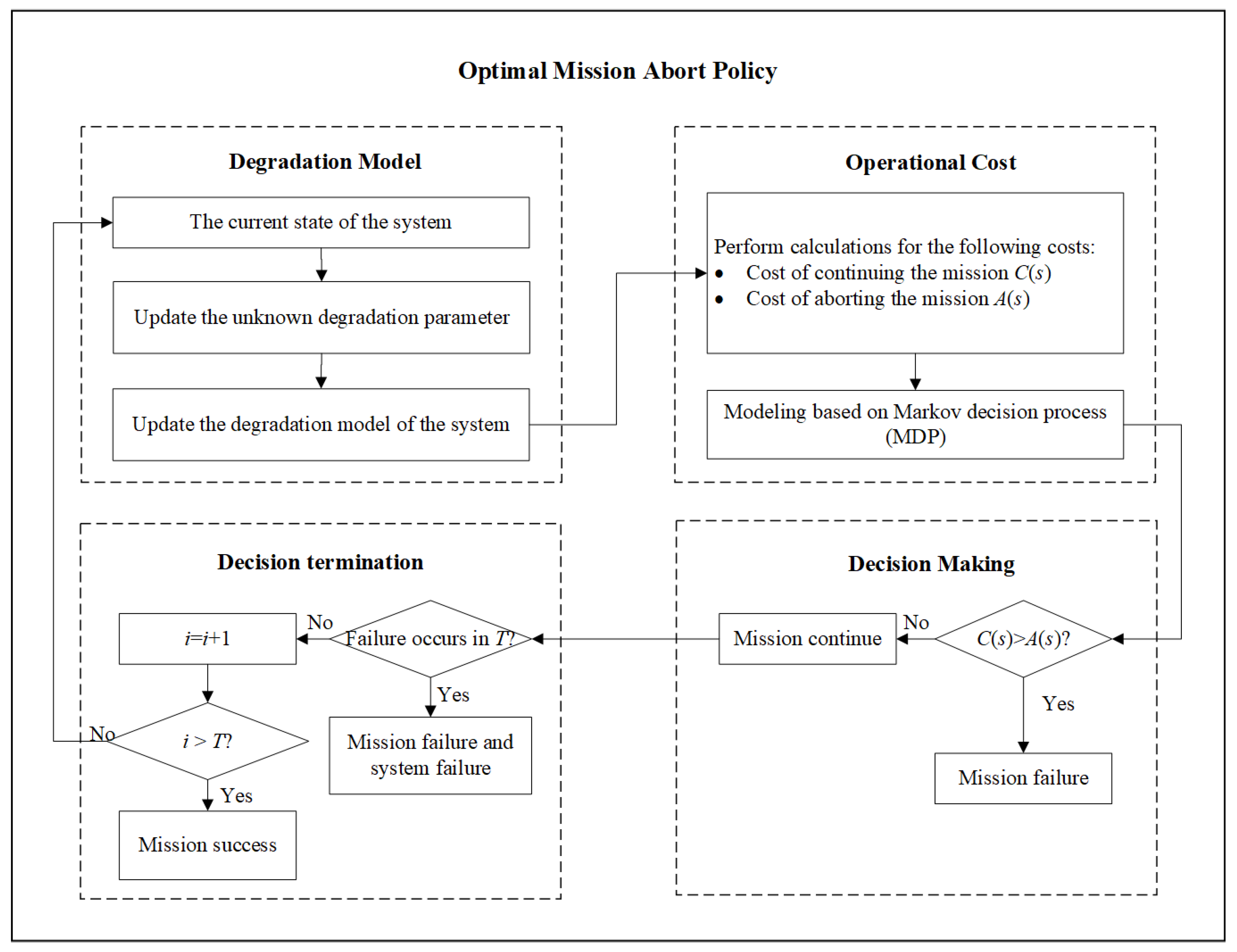
  • In order to mitigate the risk of system failure while maintaining mission reliability, an adaptive mission abort policy with integrated parameter learning is proposed, offering a significant advancement over static models. This strategy enables the dynamic adjustment of the abort decision based on the current state of the system.
  • The optimal mission abort policy is characterized as an optimal control limit policy. The monotonicity of the value function is examined, and the existence and monotonicity of the optimal abort threshold are established.
The remainder of the paper is structured as follows: In Section 2, we employ an online parameter learning approach to model the cumulative shock degradation process, taking into account heterogeneity. Section 3 introduces the optimal mission abort problem into the MDP framework. Section 4 presents the optimal mission abort policy and investigates its structural properties. Comparative policies are presented and evaluated in Section 5. Section 6 presents a series of numerical examples to illustrate the practical applicability of the optimal policy. The paper concludes with Section 7.

2. Compound Poisson Process with Heterogeneity

We investigate the problem of mission risk control for a safety-critical system that performs a mission of duration T. The system operates in a random shock environment; that is, the system degrades with the arrival of random shocks. The shocks arrive as a Poisson process, where the Poisson intensity of the shock arrival is denoted by λ . The amount of random damage caused by each shock is characterized by an inverse Gaussian distribution:
f y μ , σ = σ 2 π y 3 exp σ y μ 2 2 μ 2 y ,
where σ > 0 is the shape parameter that controls the degradation volatility, and μ > 0 is the position parameter controlling the degradation rate. The inverse Gaussian process has good mathematical properties and is similar to the Gamma process with monotonous degradation paths. Thus, the system degradation process is a compound Poisson process.
When the system degradation level exceeds a specific threshold L, we consider the system to have failed. Since the degradation state of the system cannot be directly observed except for the failure state, we can discover the degradation level of the system and the total number of shocks experienced through condition monitoring. To simplify our analysis, we assume that condition monitoring takes place at regular intervals, each set to one unit of time. Considering that the length of the mission performed by the system is T, the maximum number of inspections is T.
In practice, different individual systems typically exhibit different degradation patterns that are influenced by various factors, including manufacturing and assembly variability, material fatigue, wear, and environmental conditions. These factors contribute to the unique degradation profiles observed in different systems. Considering the effect of heterogeneity, we assume that the inverse Gaussian distribution parameter μ is stochastic. To accurately estimate the parameter, we use a dynamic Bayesian approach to infer the random variable μ . Specifically, since μ 1 represents the reciprocal of the degradation rate, which should be positive, a truncated normal distribution is chosen to ensure that all values in the priors are positive. This helps to avoid unreasonable negative estimates of the model while still maintaining the advantages of the conjugate priors. Therefore, it is assumed that the prior distribution of μ 1 follows a truncated normal distribution T N m 0 , s 0   2 .
f μ 1 m 0 , s 0   2 = s 0 ϕ s 0 μ 1 m 0 1 Φ m 0 s 0 = s 0 ϕ s 0 μ 1 m 0 Φ m 0 s 0 ,
where ϕ and Φ are the probability density function (PDF) and cumulative distribution function (CDF) of the standard normal distribution, respectively. The prior distribution can be obtained from historical data.
Since the system performs one inspection per time unit, at the i-th inspection ( i = 1 , 2 , , T ), it is possible to observe the degradation level of the system, X i , and the total number of shocks experienced, N i . Let X 1 : i : = X 1 , , X i denote a sequence of the observed degradation levels and N 1 : i : = N 1 , , N i represent the sequence of the observed total number of shocks. Then, given the observations X 1 : i and N 1 : i , the posterior distribution of the parameter μ 1 can be updated using a Bayesian approach, as shown in Proposition 1.
Proposition 1. 
Given the observed system degradation levels,  X 1 : i , and the total number of shocks up to the i-th inspection,  N 1 : i , the posterior distribution of  μ 1  is a truncated normal distribution  μ 1 T N σ N i + s 0   2 m 0 σ X i + s 0   2 , 1 σ X i + s 0   2 .
The proof of Proposition 1 is given in Appendix A. Proposition 1 states that at the i-th inspection, the posterior distribution of the parameter μ 1 depends only on the system degradation level, X i , and the total number of shocks suffered, N i . Thus, we can determine the posterior predictive distribution of the observed degradation level of the system at the i-th inspection moment, X i + 1 , based on the observed degradation signal.
Lemma 1. 
Given the observed system degradation levels,  X 1 : i , and the total number of shocks suffered  N 1 : i  up to the i-th inspection moment, the posterior predictive distribution of the system degradation level  X i + 1  at the next inspection moment can be expressed as
f X i + 1 = x N 1 : i , X 1 : i = k = 0 + λ k e λ k ! k 2 σ 2 π x X i 3 s i   2 s ^ i   2 Φ m ^ i s ^ i Φ m i s i exp m ^ i   2 s ^ i   2 m i   2 s i   2 2 k 2 σ 2 x X i ,
where  m i = σ N i + s 0   2 m 0 σ X i + s 0   2 ,  s i   2 = σ X i + s 0   2 ,  m ^ i = σ N i + k + s 0   2 m 0 σ x + s 0   2 , and  s ^ i   2 = σ x + s 0   2 .
The proof of Lemma 1 is shown in Appendix B. Lemma 1 constructs the posterior predictive distribution for the next observed degradation level of the system at the i-th inspection moment based on the current degradation level and the total number of shocks. Thus, the degradation process remains Markovian in nature, and its evolution is caused by the degradation trajectory of the current system.

3. Mission Abort Problem for Heterogeneity Degradation

For safety-critical systems performing a mission of fixed duration, the degradation process obeys the assumptions made in the previous section, and in order to control the risk of system failure while improving mission reliability, the mission can be aborted as soon as the level of system degradation exceeds a certain level. Let c I denote the inspection cost, c f represent the system failure cost, and c m indicate the mission failure cost. The choice of the mission abort threshold is the crux of the matter. Higher mission abort thresholds reduce the system reliability and lead to higher expected system failure costs; however, lower abort thresholds reduce the mission completion probability and increase expected mission failure costs. Therefore, our goal is to determine the optimal mission abort threshold for each inspection to minimize the expected total cost of inspections, system failures, and mission failures.
According to the model assumptions of the previous section, a system inspection is performed every unit of time, and at the i-th inspection, the total number of shocks experienced n and the system degradation level x are observed. Thus, i , n , x forms a discrete-time Markov chain with continuous states. Thus, the optimal mission abort policy can be formulated as a finite-horizon discrete-time Markov decision process (MDP). Specifically, at the i-th inspection moment, i = 0 , 1 , , T , and the total number of shocks and the degradation level are revealed, which are denoted by i , n , x and constitute the state of the MDP. In each state, an action can be chosen from C , A , where C denotes continuing the mission and A represents aborting the mission. If the system degradation level exceeds the failure threshold L, the total cost of system failure and mission failure, c f + c m , is incurred. If the system is in state i , n , x with x L , and action A is chosen, only the mission failure cost, c m , is incurred. Let A i , n , x denote the expected cost of aborting the mission when the system is in state i , n , x ; then, A i , n , x = c m . However, at this point, if action C is chosen, nothing will be done, while decision making will be postponed until the next inspection. Until the next inspection, the system may enter a failure state. The reliability of the system when it is in state i , n , x is
R i , n , x = Pr X i + 1 L N i = n , X i = x = x L k = 0 + λ k e λ k ! k 2 σ 2 π x x 3 s i   2 s ^ i   2 Φ m ^ i s ^ i Φ m i s i exp m ^ i   2 s ^ i   2 m i   2 s i   2 2 k 2 σ 2 x x d x ,
where m i = σ n + s 0   2 m 0 σ x + s 0   2 , s i   2 = σ x + s 0   2 , m ^ i = σ n + k + s 0   2 m 0 σ x + s 0   2 and s ^ i   2 = σ x + s 0   2 . If no failure occurs before the next inspection, the system transfers to state i + 1 , n , x . The transition probability density from state i , n , x to state i + 1 , n , x is
f i + 1 , n , x i , n , x = f N i + 1 = n , X i + 1 = x N i = n , X i = x = f X i + 1 = x N i + 1 = n , N i = n , X i = x P N i + 1 = n N i = n , X i = x = λ n n e λ n n ! n n 2 σ 2 π x x 3 s i   2 s ^ i   2 Φ m ^ i s ^ i Φ m i s i exp m ^ i   2 s ^ i   2 m i   2 s i   2 2 n n 2 σ 2 x x ,
where m i = σ n + s 0   2 m 0 σ x + s 0   2 , s i   2 = σ x + s 0   2 , m ^ i = σ n + s 0   2 m 0 σ x + s 0   2 , and s ^ i   2 = σ x + s 0   2 . Let C i , n , x represent the expected cost of continuing the mission; then, it is equal to
C i , n , x = E V i + 1 , n , x i , n , x = c I + c f + c m 1 R i , n , x + n = n + x L V i + 1 , n , x f i + 1 , n , x i , n , x d x .
Define V i , n , x as the minimal expected total cost with initial state i , n , x . Then, the value function V i , n , x satisfies the following Bellman equation:
V i , n , x = min A i , n , x , C i , n , x , x L , c f + c m , x > L .
Here A i , n , x = c m and C i , n , x can be obtained from Equation (6).
If the system does not fail until the mission is completed, it obtains a mission completion reward, r. Otherwise, it incurs the total cost of system failure and mission failure. Therefore, the boundary condition is
V T , n , x = r , x L , c f + c m , x > L .
Based on the value function and decision scheme established above, the flowchart for optimal decision making is shown in Figure 1.

4. Structural Properties

In this section, we delve into exploring the structural properties of the optimal mission abort policy. Our investigation begins with establishing the structural characteristics of the value function. Subsequently, we move on to confirming the existence and monotonic behavior of the optimal mission abort policy based on these properties. We first determine the monotonicity of the predicted degradation level, X i + 1 , for the next inspection. Before doing so, we recall the following two definitions:
Definition 1. 
A random variable X is stochastically larger than a random variable Y in the usual stochastic order, denoted by  X s t Y , if, and only if,  Pr X > t Pr Y > t  for all t.
Definition 2. 
Let X and Y be continuous random variables with probability densities f and g, respectively, such that  g t f t  increases in t over the union of the supports of X and Y, or, equivalently,  f x g y f y g x , for all  x y . Then, X is said to be smaller than Y in the likelihood ratio order, denoted by  X l r Y .
Note that the likelihood ratio order is stronger than the usual stochastic order; as such, if  X l r Y , then  X s t Y .
Proposition 2. 
The random variable  X i + 1 N i = n , X i = x  is stochastically increasing in x in the usual stochastic order.
The proof of Proposition 2 can be found in Appendix C. Proposition 2 suggests that with a fixed inspection moment and total number of shocks, an increase in the system degradation level at the current moment will correspond to a higher expected degradation level at the next inspection moment. Intuitively, a higher degradation level implies faster system degradation, leading to an anticipated larger increment of degradation in the future. Drawing on Proposition 2, Lemma 2 establishes the monotonicity of the optimal value function. This monotonic relationship underscores the importance of system degradation levels in shaping optimal decision-making processes.
Lemma 2. 
The optimal value function  V i , n , x  is a nondecreasing function of x, and a nonincreasing function of i.
The proof of Lemma 2 is given in Appendix D. Lemma 2 illustrates that when the total number of shocks at the same inspection moment is given, a higher system degradation level leads to an increase in the expected costs. Conversely, given the total number of shocks and the system degradation level, the higher the number of system inspections at the current moment, the lower the expected cost. Building on Lemma 2, we can further investigate the existence of optimal mission abort thresholds.
Theorem 1. 
At the i-th inspection epoch, for a given total number of shocks n, there exists a threshold  x i , n  such that the optimal decision is to continue the mission if  x x i , n  and to abort the mission if  x > x i , n . The abort threshold  x i , n  is a nondecreasing function of i.
The proof of Theorem 1 is presented in Appendix E. Theorem 1 establishes the existence of the optimal control threshold for a fixed total number of shocks at the same inspection moment. When the system degradation level exceeds the abort threshold, it is advisable to abort the mission. This is because with a higher system degradation level, the probability of system and mission failure increases, making it preferable to abort the mission to avoid the high penalty cost associated with failure. Additionally, Theorem 1 proves the monotonicity of the abort threshold with respect to the number of inspections. This is due to the fact that as the mission nears completion, the probability of system failure and mission failure decreases, and therefore a higher level of degradation is acceptable.
Corollary 1. 
The abort threshold  x i , n  is nonincreasing as the system failure cost  c f  increases, and nondecreasing as the mission failure cost  c m  increases.
The proof of Corollary 1 can be found in Appendix F. Corollary 1 proves the monotonicity of the optimal abort threshold with respect to the cost parameters. When the system failure cost is high, it is optimal to choose to abort the mission at a lower degradation level in order to reduce the risk of system failure. Conversely, when the mission failure cost is high, a higher mission abort threshold should be set to avoid mission failure.
Theorem 2. 
For a given level of system degradation x and total number of shocks n, there exists a threshold  i n , x  such that the optimal decision is to abort the mission if  i i n , x  and to continue the mission if  i > i n , x . The abort threshold  i n , x  is a nondecreasing function of x.
The proof of Theorem 2 is similar to Theorem 1. Theorem 2 asserts the existence of the optimal abort threshold under a fixed total number of shocks and system degradation level. It demonstrates that when the system degrades to a certain level, opting for a mission abort becomes optimal if the completed inspections are below the abort threshold. This decision is driven by the higher risk of system failure at lower inspection counts, making an early mission abort the favorable choice to prevent the significant costs associated with system and mission failures. Moreover, Theorem 2 establishes the monotonic relationship of the abort threshold with the system degradation level. A higher system degradation level signifies diminished mission reliability, prompting an early mission abort to ensure the mission’s success.
Corollary 2. 
The abort threshold  i n , x  is nondecreasing as the system failure cost  c f  increases, and nonincreasing as the mission failure cost  c m  increases.
Corollary 2, similarly to Corollary 1, confirms the monotonic relationship between the optimal mission abort threshold and the cost parameters. As the cost of system failure increases, it necessitates earlier mission aborts to reduce system failure risk. Conversely, with higher costs associated with mission failure, delaying the mission abort becomes favorable to increase the likelihood of mission completion. This adaptive strategy ensures that decision making adjusts in response to changing cost dynamics, optimizing mission outcomes accordingly.

5. Comparative Policies

In this section, we provide several heuristic mission abort policies as comparisons and construct the value function under each comparison policy.

5.1. Offline Parameter Learning Approach (Policy 1)

Under this policy, parameter heterogeneity and real-time degradation signals are disregarded. The decision maker is able to obtain a point estimate, μ ˜ , of the parameter μ based on the observed degradation signal using a maximum likelihood estimation (MLE) method. At the i-th inspection moment, given the observation state i , n , x , the point estimate μ ˜ i of parameter μ is μ ˜ i = x n .
Under this assumption, the reliability of the system when it is in state i , n , x and the transition probability density from state i , n , x to state i + 1 , n , x are, respectively:
R i , n , x = Pr X i + 1 L i , n , x = x L k = 0 + λ k e λ k ! k 2 σ 2 π x x 3 exp σ x x k μ ˜ i 2 2 μ ˜ i   2 x x d x = x L k = 0 + λ k e λ k ! k 2 σ 2 π x x 3 exp σ n x / x 1 k 2 2 x x d x
f i + 1 , n , x i , n , x = f N i + 1 = n , X i + 1 = x N i = n , X i = x = λ n n e λ n n ! n n 2 σ 2 π x x 3 exp σ x x n n μ ˜ i 2 2 μ ˜ i   2 x x = λ n n e λ n n ! n n 2 σ 2 π x x 3 exp σ n x / x 1 n n 2 2 x x
Therefore, the value function under this policy is
V i , n , x = min A i , n , x , C i , n , x , x L , c f + c m , x > L , = min c m , c I + c f + c m L + k = 0 + λ k e λ k ! k 2 σ 2 π x x 3 exp σ n x / x 1 k 2 2 x x d x + n = n + x L V i + 1 , n , x λ n n e λ n n ! n n 2 σ 2 π x x 3 exp σ n x / x 1 n n 2 2 x x d x , x L , c f + c m , x > L .

5.2. Fixed Abort Threshold (Policy 2)

With this policy, the heterogeneity of the degradation parameter is still taken into account when modeling the cumulative degradation process. However, in contrast to the optimal policy proposed in this paper, this policy assumes that the mission abort threshold, denoted by l, is fixed. In other words, the mission is terminated as soon as the observed degradation level exceeds the threshold l at each decision point. In consequence of the aforementioned assumption, the value function is
V i , n , x = C i , n , x , x l , A i , n , x , l < x L , c f + c m , x > L ,
Here, A i , n , x = c m , and C i , n , x can be obtained from Equation (6).

6. Numerical Experiment

In this section, we delve into the application of the proposed optimal mission abort policy to unmanned aerial vehicles (UAVs), which play a crucial role in modern technology and military operations. The typical structure of a UAV, as depicted in Figure 2 [53], showcases its intricate design. UAVs are prized for their high mobility, cost-effectiveness, and the absence of risk to human lives, making them indispensable for tasks like reconnaissance, surveillance, logistics, transportation, and disaster relief efforts. However, as safety-critical systems, UAVs are continually exposed to various shocks during flight, ranging from airflow disruptions and mechanical vibrations to bird collisions and abrupt weather changes. These shocks can result in fatigue, wear, and potential structural or component failure within the UAVs. Given these challenges, developing a robust mission abort policy for UAVs is vital to safeguard mission success and to mitigate damage in dynamic and demanding operational environments.

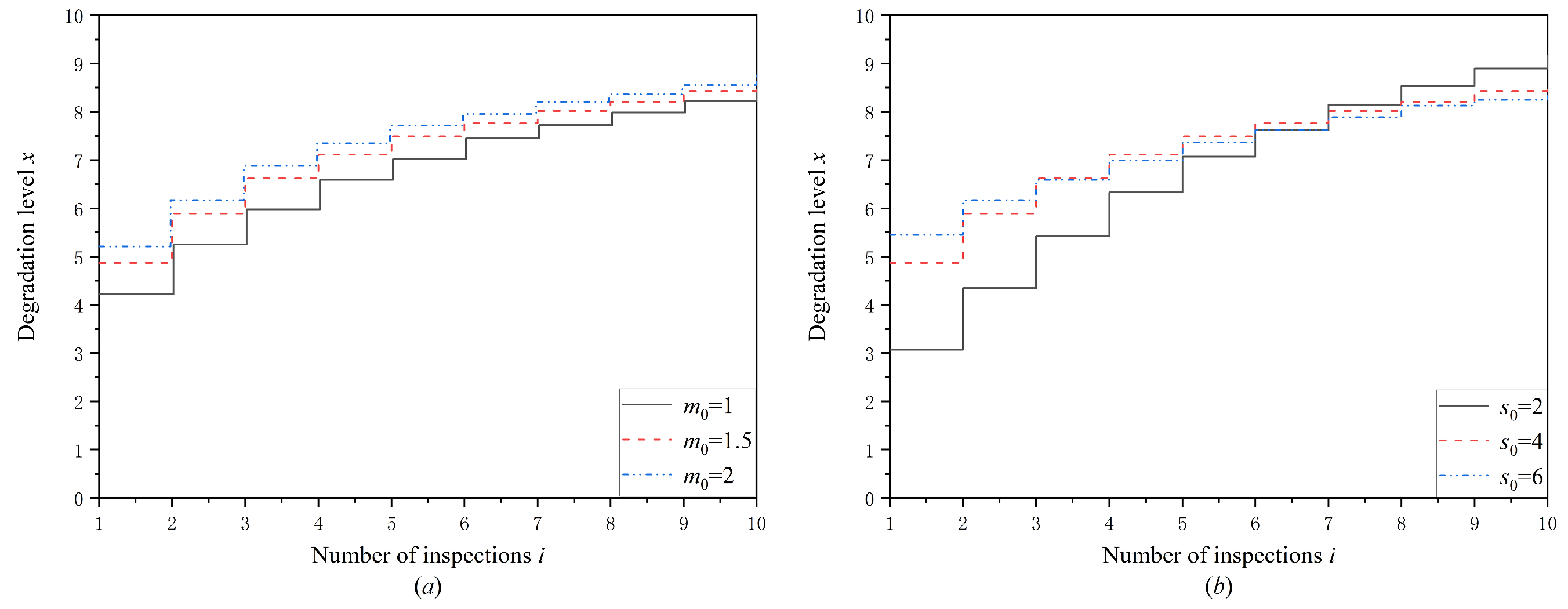
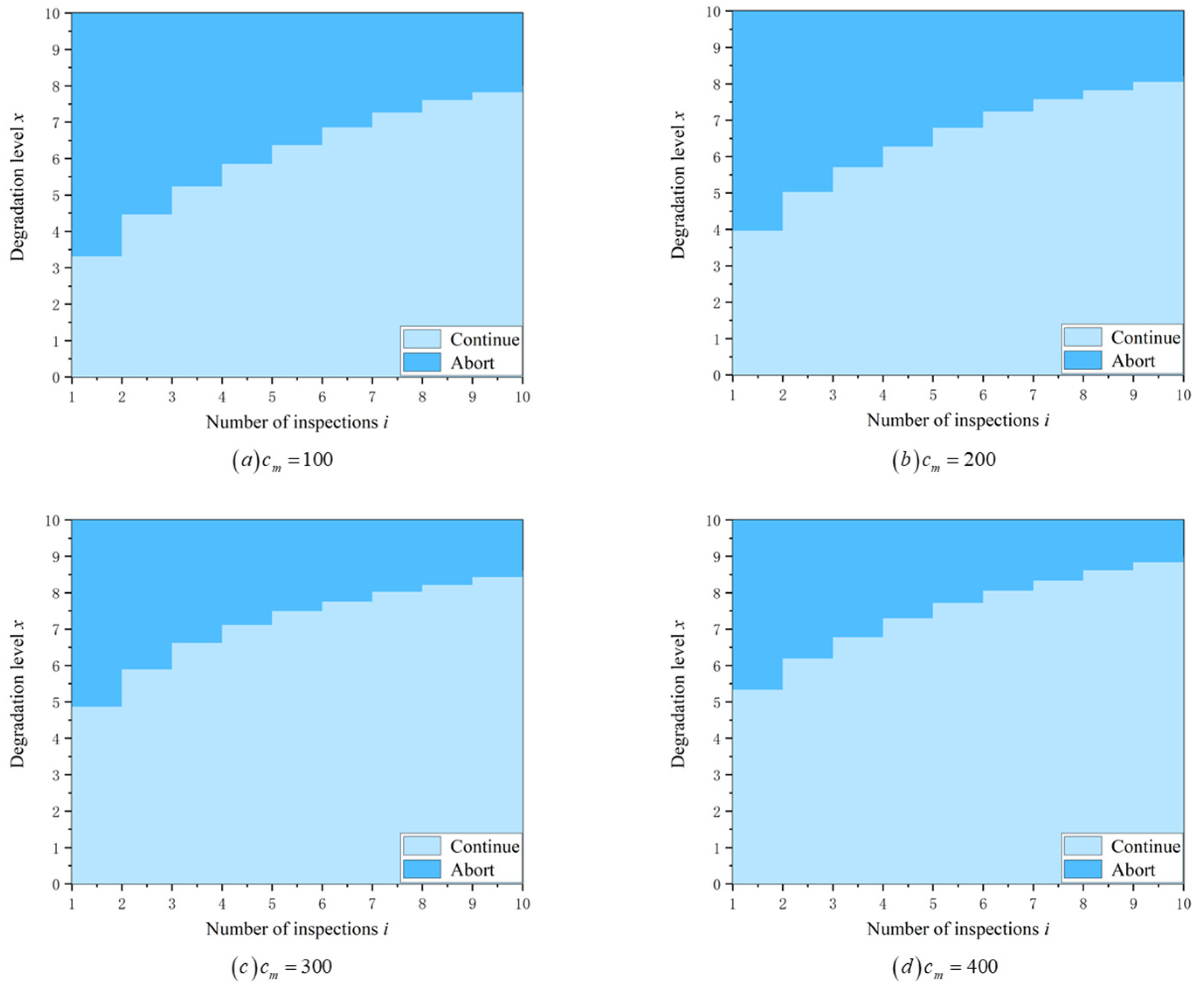
6.1. Optimal Mission Abort Policy

The degradation process of the UAV is modeled using the compound Poisson process assumed in this paper. Shock arrivals follow a Poisson process with an arrival rate of λ = 2 . The damage to the UAV caused by each shock follows an inverse Gaussian distribution, where the shape parameter σ = 0.1 and the position parameter μ is unknown. The prior distribution of the parameter μ 1 follows a truncated normal distribution, i.e., μ 1 T N m 0 , s 0   2 , where m 0 = 1.5 , s 0 = 4 . The failure threshold of the system is D = 10 . The maximum number of inspections during the mission of the UAV is T = 10 . The costs of periodic inspection, system failure, and mission failure are USD 200, USD 100,000 and USD 30,000, respectively. In the following, we abbreviate the cost parameters as c I = 2 , c f = 1000 , and c m = 300 , respectively.
Based on the current parametric assumptions, we conducted numerical experiments on the proposed optimal task abort policy. Figure 3 shows the existence and monotonicity of the optimal abort threshold for different hyperparameter settings. As can be seen in Figure 3, under different hyperparameter assumptions, the optimal action is to abort the mission if the degradation level is higher than the optimal abort threshold x i , n at each decision time. When the system is degraded to the same level, the optimal action is to abort the mission if the current number of inspections is less than the optimal threshold i n , x . In addition, it can be seen in Figure 3 that the threshold x i , n increases with the number of inspections i, and the threshold i n , x increases with the degradation level x. This is consistent with the conclusions obtained above.
Also, Figure 3a illustrates the optimal policy for varying values of m 0 when s 0 = 4 . From Figure 3a, it can be observed that when the hyperparameter m 0 is larger, the abort threshold at the early inspection moment is higher. This is because the available system degradation signals at an earlier moment are limited, and at this time, the degradation modeling and decision making depend more on the hyperparameter settings. Therefore, an elevated parameter m 0 is correlated with a diminished parameter μ , indicating that the system degradation rate is relatively low and thus capable of withstanding a greater degradation level. However, at subsequent inspection stages, an increase in the number of observed degradation signals indicates a reduction in the influence of the hyperparameter m 0 on decision-making processes. Therefore, the abort threshold gradually converges as the inspection progresses. Furthermore, Figure 3b illustrates the optimal abort strategy when m 0 = 1.5 with varying values of the hyperparameter s 0 . As observed in Figure 3b, the smaller the hyperparameter s 0 , the greater the variability in the abort threshold. As the value of s 0 decreases, the variance of the parameter μ increases, resulting in a greater degree of heterogeneity. However, as the examination continues, the impact of the hyperparameter on the abort decision gradually diminishes, resulting in a gradual convergence of the abort threshold.
Figure 4 shows the optimal actions corresponding to the same total number of shocks for different settings of the mission failure cost. From each of the plots in Figure 4, we can observe that it is preferable to choose to abort the mission at the same inspection moment when the total number of shocks is fixed and when the degradation level of the system is higher than the optimal abort threshold x i , n . When the degradation level and the total number of shocks of the system are fixed, it is preferable to choose to abort the mission if the number of inspections of the system at the current moment is less than the optimal threshold i n , x . Also, as can be seen from Figure 4, at the same inspection moment, as the mission failure cost increases from 100 to 400, the threshold corresponding to the degradation level keeps increasing. However, when the system reaches the same degradation level, the threshold corresponding to the number of inspections decreases with the increase in mission failure cost. This is because as the mission failure cost increases, the importance of mission success continues to increase in order to obtain a smaller expected total cost. Therefore, to increase the probability of mission completion, longer mission durations and higher degradation levels can be accepted.
Figure 5 depicts the presence and monotonic behavior of the optimal abort threshold. Importantly, the graph showcases a notable trend where, with an increase in the cost of system failure, the abort threshold related to the number of inspections rises, while the threshold associated with the degree of degradation decreases. This observed pattern reflects a strategic shift—when confronted with higher system failure costs, prioritizing system survivability over mission completion becomes imperative. Consequently, to enhance system reliability, preemptive mission aborts at lower degradation levels are preferred to avoid the risk of failure.

6.2. Comparison with Other Policies

In this subsection, we conducted a comparative analysis of the optimal policy proposed in this paper against two other heuristic methods. Table 1 and Table 2 present a comparison of the total cost incurred by the optimal policy and the alternative heuristics across various cost parameter configurations. The findings reveal that the offline parameter learning approach policy (Policy 1) outperforms the fixed abort threshold policy (Policy 2). This superiority stems from Policy 1’s utilization of dynamic thresholding informed by real-time system degradation data, in contrast to Policy 2’s reliance on a static abort threshold, which may result in substantial losses from system and mission failures. Furthermore, Table 2 highlights that as the system failure cost rises, the disparity in total costs between the optimal policy and the heuristics becomes more pronounced. Hence, the optimal policy demonstrates markedly superior performance, especially in scenarios with elevated system failure costs.

7. Conclusions

This paper delves into the optimization of mission abort policies while considering cumulative shock degradation. The system operates in a shock environment where the shock arrivals follow a Poisson distribution, and the random damage caused by each shock follows an inverse Gaussian distribution with an unknown position parameter. By employing the global Bayesian method for online parameter learning based on real-time degradation signals, the research enhances the precision of estimating the unknown parameter. Within the framework of MDP, the paper formulates a mission abort policy that integrates parameter learning to manage system failure risks effectively. Structural properties of the optimal abort policy are analyzed, defining it as a control limit policy. Furthermore, the study delves into investigating the existence and monotonic nature of the optimal abort threshold. Through comparative analysis with heuristic approaches, the superior efficacy of the optimal policy in enhancing system reliability and reducing failure risks is underscored.
This study lays the groundwork for potential extensions in future research endeavors. While the current focus addresses the uncertainty of shock damage, forthcoming studies could explore the joint influence of both uncertain shock arrival rates and damage, paving the way for a more holistic system degradation modeling approach that considers dynamic environmental factors. Moreover, while the study delves into a single-mission abort policy, there is room for future investigations to broaden the scope to phased mission abort policies. This extension holds promise for offering insights into tackling the intricacies of phased missions in practical applications, enhancing strategies to better align with real-world operational scenarios.

Author Contributions

Methodology, Y.M.; formal analysis, Y.M.; resources, X.M. and L.Y.; writing—original draft preparation, Y.M.; writing—review and editing, F.W., Q.Q. and L.Y.; visualization, Y.M.; supervision, X.M. and Q.Q.; funding acquisition, L.Y. All authors have read and agreed to the published version of the manuscript.

Funding

This research was funded by the National Natural Science Foundation of China (Grant No. 72101010).

Data Availability Statement

No new data were created or analyzed in this study. Data sharing is not applicable to this article.

Conflicts of Interest

The authors declare no conflict of interest.

Appendix A

Proof of Proposition 1. 
Assume that the total number of shocks between the (i-1)-th and the i-th inspection is denoted as K i , and the amount of damage caused by the j-th shock between the (i-1)-th inspection and the i-th inspection is denoted as Y i j . Then, let Y i : = Y i 1 , , Y i K i . Thus, given μ 1 , the joint likelihood of observations N 1 : i and X 1 : i is
L N 1 : i , X 1 : i μ 1 = l = 1 i λ K l e λ K l ! j = 1 K l σ 2 π Y l j 3 exp σ Y l j μ 2 2 μ 2 Y l j = l = 1 i λ K l e λ K l ! j = 1 K l σ 2 π Y l j 3 exp l = 1 i j = i K l σ μ 1 Y l j 1 2 2 Y l j
This yields
f μ 1 | N 1 : i , X 1 : i = L N 1 : i , X 1 : i | μ 1 f μ 1 m 0 , s 0   2 L N 1 : i , X 1 : i | μ 1 f μ 1 m 0 , s 0   2 d μ 1 = l = 1 i λ K l e λ K l ! j = 1 K l σ 2 π Y l j 3 exp l = 1 i j = i K l σ μ 1 Y l j 1 2 2 Y l j s 0 ϕ s 0 μ 1 m 0 Φ m 0 s 0 0 + l = 1 i λ K l e λ K l ! j = 1 K l σ 2 π Y l j 3 exp l = 1 i j = i K l σ μ 1 Y l j 1 2 2 Y l j s 0 ϕ s 0 μ 1 m 0 Φ m 0 s 0 d μ 1 = σ X i + s 0   2 2 π exp σ X i + s 0   2 2 μ 1 σ N i + s 0   2 m 0 σ X i + s 0   2 0 + σ X i + s 0   2 2 π exp σ X i + s 0   2 2 μ 1 σ N i + s 0   2 m 0 σ X i + s 0   2 d μ 1 = σ X i + s 0   2 ϕ σ X i + s 0   2 μ 1 σ N i + s 0   2 m 0 σ X i + s 0   2 Φ σ N i + s 0   2 m 0 σ X i + s 0   2 σ X i + s 0   2
Apparently, the posterior distribution of μ 1 is also a truncated normal distribution, which can be denoted as T N m i , s i   2 , where m i = σ N i + s 0   2 m 0 σ X i + s 0   2 , and s i   2 = σ X i + s 0   2 . □

Appendix B

Proof of Lemma 1. 
We first consider the posterior predictive distribution conditioned on the shock number increment K i :
f X i + 1 = x K i = k , N 1 : i , X 1 : i = 0 + f k x X i μ 1 f μ 1 N 1 : i , X 1 : i d μ 1 = 0 + k 2 σ 2 π x X i 3 exp k 2 σ x X i k μ 2 2 k 2 μ 2 x X i s i ϕ s i μ 1 m i Φ m i s i d μ 1 = k 2 σ 2 π x X i 3 s i   2 s ^ i   2 Φ m ^ i s ^ i Φ m i s i exp m ^ i   2 s ^ i   2 m i   2 s i   2 2 k 2 σ 2 x X i
where m i = σ N i + s 0   2 m 0 σ X i + s 0   2 , s i   2 = σ X i + s 0   2 , m ^ i = σ N i + k + s 0   2 m 0 σ x + s 0   2 , and s ^ i   2 = σ x + s 0   2 .
Thus, the posterior predictive distribution of the random variable X i + 1 is
f X i + 1 = x N 1 : i , X 1 : i = k = 0 + f X i + 1 = x K i = k , N 1 : i , X 1 : i P K i = k = k = 0 + λ k e λ k ! k 2 σ 2 π x X i 3 s i   2 s ^ i   2 Φ m ^ i s ^ i Φ m i s i exp m ^ i   2 s ^ i   2 m i   2 s i   2 2 k 2 σ 2 x X i
Thus, we complete the proof. □

Appendix C

Proof of Proposition 2. 
We consider two different degradation levels, x 1 and x 2 ( x 1 < x 2 ), at the same inspection epoch i in which we observed the same total number of shocks n. For any 0 < μ 1   1 < μ 2   1 , we have the likelihood ratio
f y μ 2   1 f y μ 1   1 = exp σ y μ 2 2 2 μ 2   2 y + σ y μ 1 2 2 μ 1   2 y = exp σ y 2 μ 1   2 μ 2   2 σ μ 1   1 μ 2   1
Since μ 1   1 < μ 2   1 , the ratio is decreasing in y. This yields the likelihood ratio order and, as a consequence, the usual stochastic order. This now reveals that the random variables Y μ 1 = Y μ 1 are stochastically decreasing in μ 1 , i.e., μ 1   1 < μ 2   1 implies Y μ 1   1 s t Y μ 2   1 .
Then, for x 1 < x 2 , consider the likelihood ratio
f μ 1 x 2 f μ 1 x 1 = s i , 2   2 s i , 1   2 Φ m i , 1 s i , 1 Φ m i , 2 s i , 2 exp s i , 2   2 μ 1 m i , 2 2 / 2 exp s i , 1   2 μ 1 m i , 1 2 / 2
where s i , 1   2 = σ x 1 + s 0   2 , m i , 1 = σ n + s 0   2 m 0 σ x 1 + s 0   2 , s i , 2   2 = σ x 2 + s 0   2 , and m i , 2 = σ n + s 0   2 m 0 σ x 2 + s 0   2 .
Thus, we have
f μ 1 x 2 f μ 1 x 1 exp s i , 1   2 s i , 2   2 2 μ 2 s i , 1   2 m i , 1 s i , 2   2 m i , 2 μ 1 = exp σ x 1 x 2 2 μ 2
Since x 1 < x 2 , the ratio is decreasing in μ 1 . Thus, we can determine that μ 1 x 1 s t μ 1 x 2 . Thus, from the stochastic monotonicity of Y μ 1 , the above yields Y x 1 : = Y μ 1 x 1 s t Y μ 1 x 2 : = Y x 2 . Finally, it is evident that
X i + 1 x 1 : = x 1 + k = 1 K i + 1 Y k x 1 s t x 2 + k = 1 K i + 1 Y k x 2 : = X i + 1 x 2
In conclusion, the random variable X i + 1 N i = n , X i = x is stochastically increasing in x. □

Appendix D

Proof of Lemma 2. 
We first prove the monotonicity of the value function on x. By Proposition 2, we show that X i + 1 N i = n , X i = x is stochastically increasing in x. Then, we use a recursive algorithm to prove the monotonicity of the value function. Obviously, V T , n , x is a nondecreasing function of x. Now assume that V j , n , x is a nondecreasing function of x for all j T and n > 0 : then, for x 1 < x 2 , it follows that
V j 1 , n , x 1 = min c m , E V j , N j , X j | N j 1 = n , X j 1 = x 1 min c m , E V j , N j , X j | N j 1 = n , X j 1 = x 2 = V j 1 , n , x 2
Thus, V j 1 , n , x is a nondecreasing function of x. Therefore, combined with the recursive process, we can prove that V i , n , x is a nondecreasing function of x.
Next, we prove the monotonicity of the value function on i. Similarly, we assume that V i , n , x is a nonincreasing function in i; thus, for V i 1 , n , x , we have
V i , n , x = min c m , E V i + 1 , N i + 1 , X i + 1 | N i = n , X i = x min c m , E V i , N i , X i | N i 1 = n , X i 1 = x = V i 1 , n , x
Therefore, combined with the recursive process, we can prove that the value function V i , n , x is a nonincreasing function of i. □

Appendix E

Proof of Theorem 1. 
By Lemma 1, C i , n , x is a nondecreasing function of x. Also, considering A i , n , x = c m , we can determine that for x 1 < x 2 ,
C i , n , x 1 C i , n , x 2 A i , n , x 1 A i , n , x 2 = 0
Therefore, the following inequality holds:
C i , n , x 1 A i , n , x 1 C i , n , x 2 A i , n , x 2
Thus, for a given i and n, there exists a threshold x i , n that satisfies the following: for x x i , n , the optimal action is to continue the mission; for x > x i , n , the optimal action is to abort the mission.
Next, we prove the monotonicity of x i , n . If there exists j such that C j , n , x A j , n , x , then since C i , n , x is a nonincreasing function of i and A i , n , x = c m , it follows that for all i j , we have C i , n , x A i , n , x . That is, for all i j , we have x i , n x j , n . Thus, the abort threshold x i , n is a nondecreasing function of i. □

Appendix F

Proof of Corollary 1. 
We use the contradiction to prove the monotonicity of the threshold x i , n with respect to the costs. Assume that c f 1 and c f 2 are the two system failure costs ( c f 1 < c f 2 ), and that x 1 * i , n and x 2 * i , n are the optimal abort thresholds corresponding to these two system failure costs, respectively. Also, let C 1 i , n , x and C 2 i , n , x be the expected costs of continuing the mission under c f 1 and c f 2 , respectively. Assuming that x 1 * i , n < x 2 * i , n , it follows from Theorem 1 that for x x 2 i , n , the optimal action is to continue the mission when the system failure cost is c f 2 ; thus, we have
C 2 i , n , x 1 * i , n = c I + c f 2 + c m 1 R i , n , x 1 * i , n + n = n + x 1 * i , n L V i + 1 , n , x f i + 1 , n , x | i , n , x 1 * i , n d x < c m
In addition, considering that c f 1 < c f 2 , we obtain
C 2 i , n , x 1 * i , n = c I + c f 2 + c m 1 R i , n , x 1 * i , n + n = n + x 1 * i , n L V i + 1 , n , x f i + 1 , n , x | i , n , x 1 * i , n d x c I + c f 1 + c m 1 R i , n , x 1 * i , n + n = n + x 1 * i , n L V i + 1 , n , x f i + 1 , n , x | i , n , x 1 * i , n d x = C 1 i , n , x 1 * i , n c m
From the above two equations, we obtain C 2 i , n , x 1 * i , n < c m and C 2 i , n , x 1 * i , n c m , respectively, which is a contradiction. Thus, x 1 * i , n x 2 * i , n , i.e., x i , n is nonincreasing as the system failure cost c f increases.
Similarly, we can prove that x i , n is nondecreasing as the mission failure cost c m increases. □

References

  1. Dui, H.; Xu, H.; Zhang, Y.-A. Reliability Analysis and Redundancy Optimization of a Command Post Phased-Mission System. Mathematics 2022, 10, 4180. [Google Scholar] [CrossRef]
  2. Qiu, Q.; Maillart, L.M.; Prokopyev, O.A.; Cui, L. Optimal condition-based mission abort decisions. IEEE Trans. Reliab. 2023, 72, 408–425. [Google Scholar] [CrossRef]
  3. Shang, L.; Liu, B.; Gao, K.; Yang, L. Random Warranty and Replacement Models Customizing from the Perspective of Heterogeneity. Mathematics 2023, 11, 3330. [Google Scholar] [CrossRef]
  4. Jia, H.; Peng, R.; Yang, L.; Wu, T.; Liu, D.; Li, Y. Reliability evaluation of demand-based warm standby systems with capacity storage. Reliab. Eng. Syst. Saf. 2022, 218, 108132. [Google Scholar] [CrossRef]
  5. Zhao, X.; Li, B.; Mizutani, S.; Nakagawa, T. A Revisit of Age-Based Replacement Models With Exponential Failure Distributions. IEEE Trans. Reliab. 2022, 71, 1477–1487. [Google Scholar] [CrossRef]
  6. Kim, M.J.; Makis, V. Joint optimization of sampling and control of partially observable failing systems. Oper. Res. 2013, 61, 777–790. [Google Scholar] [CrossRef]
  7. Wu, D.; Han, R.; Ma, Y.; Yang, L.; Wei, F.; Peng, R. A two-dimensional maintenance optimization framework balancing hazard risk and energy consumption rates. Comput. Ind. Eng. 2022, 169, 108193. [Google Scholar] [CrossRef]
  8. Yang, L.; Chen, Y.; Ma, X.; Qiu, Q.; Peng, R. A Prognosis-centered Intelligent Maintenance Optimization Framework under Uncertain Failure Threshold. IEEE Trans. Reliab. 2024, 73, 115–130. [Google Scholar] [CrossRef]
  9. Wei, F.; Wang, J.; Ma, X.; Yang, L.; Qiu, Q. An Optimal Opportunistic Maintenance Planning Integrating Discrete- and Continuous-State Information. Mathematics 2023, 11, 3322. [Google Scholar] [CrossRef]
  10. Chen, Y.; Ma, X.; Wei, F.; Yang, L.; Qiu, Q. Dynamic Scheduling of Intelligent Group Maintenance Planning under Usage Availability Constraint. Mathematics 2022, 10, 2730. [Google Scholar] [CrossRef]
  11. Levitin, G.; Xing, L.; Dai, Y. Optimal system loading and aborting in additive multi-attempt missions. Reliab. Eng. Syst. Saf. 2024, 251, 110315. [Google Scholar] [CrossRef]
  12. Chen, K.; Zhao, X.; Qiu, Q. Optimal Task Abort and Maintenance Policies Considering Time Redundancy. Mathematics 2022, 10, 1360. [Google Scholar] [CrossRef]
  13. Xiao, H.; Yi, K.; Peng, R.; Kou, G. Reliability of a Distributed Computing System With Performance Sharing. IEEE Trans. Reliab. 2022, 71, 1555–1566. [Google Scholar] [CrossRef]
  14. Levitin, G.; Xing, L.; Dai, Y. Multi-attempt missions with multiple rescue options. Reliab. Eng. Syst. Saf. 2024, 248, 110168. [Google Scholar] [CrossRef]
  15. Qiu, Q.; Li, R.; Zhao, X. Failure risk management: Adaptive performance control and mission abort decisions. Risk Anal. 2024, 1–20. [Google Scholar] [CrossRef] [PubMed]
  16. Yang, L.; Wei, F.; Qiu, Q. Mission Risk Control via Joint Optimization of Sampling and Abort Decisions. Risk Anal. 2024, 44, 666–685. [Google Scholar] [CrossRef] [PubMed]
  17. Myers, A. Probability of loss assessment of critical k-out-of-n: G systems having a mission abort policy. IEEE Trans. Reliab. 2009, 58, 694–701. [Google Scholar] [CrossRef]
  18. Levitin, G.; Xing, L.; Dai, Y. Mission Abort Policy in Heterogeneous Nonrepairable 1-Out-of-N Warm Standby Systems. IEEE Trans. Reliab. 2018, 67, 342–354. [Google Scholar] [CrossRef]
  19. Levitin, G.; Xing, L.; Dai, Y. Co-optimization of state dependent loading and mission abort policy in heterogeneous warm standby systems. Reliab. Eng. Syst. Saf. 2018, 172, 151–158. [Google Scholar] [CrossRef]
  20. Wang, J.; Ma, X.; Zhao, Y.; Gao, K.; Yang, L. Condition-based maintenance management for two-stage continuous deterioration with two-dimensional inspection errors. Qual. Reliab. Eng. Int. 2024. [Google Scholar] [CrossRef]
  21. Zhao, X.; Chai, X.; Sun, J.; Qiu, Q. Optimal bivariate mission abort policy for systems operate in random shock environment. Reliab. Eng. Syst. Saf. 2021, 205, 107244. [Google Scholar] [CrossRef]
  22. Levitin, G.; Xing, L.; Xiang, Y.; Dai, Y. Mixed failure-driven and shock-driven mission aborts in heterogeneous systems with arbitrary structure. Reliab. Eng. Syst. Saf. 2021, 212, 107581. [Google Scholar] [CrossRef]
  23. Qiu, Q.; Cui, L. Gamma process based optimal mission abort policy. Reliab. Eng. Syst. Saf. 2019, 190, 106496. [Google Scholar] [CrossRef]
  24. Cheng, G.; Li, L.; Zhang, L.; Yang, N.; Jiang, B.; Shangguan, C.; Su, Y. Optimal Joint Inspection and Mission Abort Policies for Degenerative Systems. IEEE Trans. Reliab. 2023, 72, 137–150. [Google Scholar] [CrossRef]
  25. Wang, J.; Peng, R.; Qiu, Q.; Zhou, S.; Yang, L. An inspection-based replacement planning in consideration of state-driven imperfect inspections. Reliab. Eng. Syst. Saf. 2023, 232, 109064. [Google Scholar] [CrossRef]
  26. Yang, L.; Chen, Y.; Qiu, Q.; Wang, J. Risk Control of Mission-Critical Systems: Abort Decision-Makings Integrating Health and Age Conditions. IEEE Trans. Ind. Inform. 2022, 18, 6887–6894. [Google Scholar] [CrossRef]
  27. Mizutani, S.; Dong, W.; Zhao, X.; Nakagawa, T. Preventive replacement policies with products update announcements. Commun. Stat. -Theory Methods 2020, 49, 3821–3833. [Google Scholar] [CrossRef]
  28. Qiu, Q.; Kou, M.; Chen, K.; Deng, Q.; Kang, F.; Lin, C. Optimal stopping problems for mission oriented systems considering time redundancy. Reliab. Eng. Syst. Saf. 2021, 205, 107226. [Google Scholar] [CrossRef]
  29. Ma, X.; Liu, B.; Yang, L.; Peng, R.; Zhang, X. Reliability analysis and condition-based maintenance optimization for a warm standby cooling system. Reliab. Eng. Syst. Saf. 2020, 193, 106588. [Google Scholar] [CrossRef]
  30. Levitin, G.; Xing, L. Mission Aborting Policies and Multiattempt Missions. IEEE Trans. Reliab. 2024, 73, 51–52. [Google Scholar] [CrossRef]
  31. Meng, S.; Xing, L.; Levitin, G. Activation delay and aborting policy minimizing expected losses in consecutive attempts having cumulative effect on mission success. Reliab. Eng. Syst. Saf. 2024, 247, 110078. [Google Scholar] [CrossRef]
  32. Wang, J.; Tan, L.; Ma, X.; Gao, K.; Jia, H.; Yang, L. Prognosis-driven reliability analysis and replacement policy optimization for two-phase continuous degradation. Reliab. Eng. Syst. Saf. 2023, 230, 108909. [Google Scholar] [CrossRef]
  33. Levitin, G.; Finkelstein, M.; Xiang, Y. Optimal mission abort policies for repairable multistate systems performing multi-attempt mission. Reliab. Eng. Syst. Saf. 2021, 209, 107497. [Google Scholar] [CrossRef]
  34. Chen, Y.; Wu, T.; Ma, X.; Wang, J.; Peng, R.; Yang, L. System Maintenance Optimization Under Structural Dependency: A Dynamic Grouping Approach. IEEE Syst. J. 2024. [Google Scholar] [CrossRef]
  35. Yang, L.; Ye, Z.S.; Lee, C.G.; Yang, S.F.; Peng, R. A two-phase preventive maintenance policy considering imperfect repair and postponed replacement. Eur. J. Oper. Res. 2019, 274, 966–977. [Google Scholar] [CrossRef]
  36. Shang, L.; Liu, B.; Qiu, Q.; Yang, L. Three-dimensional warranty and post-warranty maintenance of products with monitored mission cycles. Reliab. Eng. Syst. Saf. 2023, 239, 109506. [Google Scholar] [CrossRef]
  37. Drent, C.; Drent, M.; Arts, J.; Kapodistria, S. Real-Time Integrated Learning and Decision Making for Cumulative Shock Degradation. Manuf. Serv. Oper. Manag. 2022, 25, 235–253. [Google Scholar] [CrossRef]
  38. Chen, N.; Tsui, K.L. Condition monitoring and residual life prediction using degradation signals: Revisited. IIE Trans. 2013, 45, 939–952. [Google Scholar] [CrossRef]
  39. Yang, L.; Peng, R.; Li, G.; Lee, C.G. Operations management of wind farms integrating multiple impacts of wind conditions and resource constraints. Energy Convers. Manag. 2020, 205, 112162. [Google Scholar] [CrossRef]
  40. Qu, L.; Liao, J.; Gao, K.; Yang, L. Joint Optimization of Production Lot Sizing and Preventive Maintenance Threshold Based on Nonlinear Degradation. Appl. Sci. 2022, 12, 8638. [Google Scholar] [CrossRef]
  41. Yang, L.; Chen, Y.; Ma, X. A State-age-dependent Opportunistic Intelligent Maintenance Framework for Wind Turbines under Dynamic Wind Conditions. IEEE Trans. Ind. Inform. 2023, 19, 10434–10443. [Google Scholar] [CrossRef]
  42. Zhang, Z.; Yang, L. Postponed maintenance scheduling integrating state variation and environmental impact. Reliab. Eng. Syst. Saf. 2020, 202, 107065. [Google Scholar] [CrossRef]
  43. Meng, S.; Xing, L.; Levitin, G. Optimizing component activation and operation aborting in missions with consecutive attempts and common abort command. Reliab. Eng. Syst. Saf. 2024, 243, 109842. [Google Scholar] [CrossRef]
  44. Wang, J.; Ma, X.; Qiu, Q.; Yang, L.; Shang, L.; Wang, J. A hybrid inspection-replacement policy for multi-stage degradation considering imperfect inspection with variable probabilities. Reliab. Eng. Syst. Saf. 2023, 241, 109629. [Google Scholar] [CrossRef]
  45. Xiao, H.; Yi, K.; Liu, H.; Kou, G. Reliability modeling and optimization of a two-dimensional sliding window system. Reliab. Eng. Syst. Saf. 2021, 215, 107870. [Google Scholar] [CrossRef]
  46. Yang, L.; Li, G.; Zhang, Z.; Ma, X.; Zhao, Y. Operations & Maintenance Optimization of Wind Turbines Integrating Wind and Aging Information. IEEE Trans. Sustain. Energy 2021, 12, 211–221. [Google Scholar]
  47. Zhao, X.; Qian, C.; Nakagawa, T. Comparisons of replacement policies with periodic times and repair numbers. Reliab. Eng. Syst. Saf. 2017, 168, 161–170. [Google Scholar] [CrossRef]
  48. Wang, J.; Yang, L.; Ma, X.; Peng, R. Joint optimization of multi-window maintenance and spare part provisioning policies for production systems. Reliab. Eng. Syst. Saf. 2021, 216, 108006. [Google Scholar] [CrossRef]
  49. Levitin, G.; Xing, L.; Dai, Y. A new self-adaptive mission aborting policy for systems operating in uncertain random shock environment. Reliab. Eng. Syst. Saf. 2024, 248, 110184. [Google Scholar] [CrossRef]
  50. Qiu, Q.; Cui, L. Optimal mission abort policy for systems subject to random shocks based on virtual age process. Reliab. Eng. Syst. Saf. 2019, 189, 11–20. [Google Scholar] [CrossRef]
  51. Zhang, Z.; Yang, L. State-Based Opportunistic Maintenance with Multifunctional Maintenance Windows. IEEE Trans. Reliab. 2021, 70, 1481–1494. [Google Scholar] [CrossRef]
  52. Wang, L.; Song, Y.; Qiu, Q.; Yang, L. Warranty Cost Analysis for Multi-State Products Protected by Lemon Laws. Appl. Sci. 2023, 13, 1541. [Google Scholar] [CrossRef]
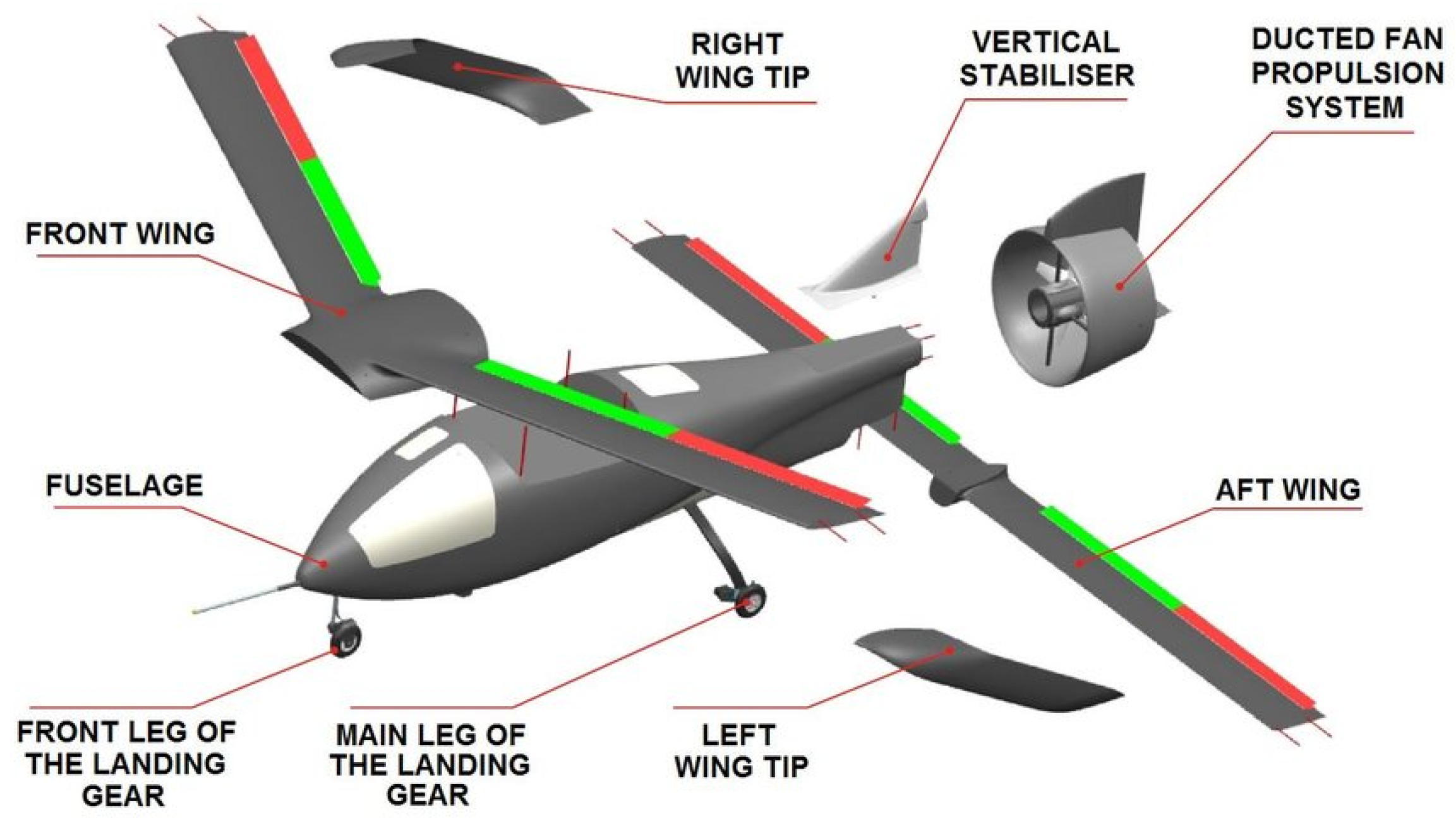
  53. Galiński, C.; Hajduk, J.; Kalinowski, M.; Wichulski, M.; Stefanek, L. Inverted joined wing scaled demonstrator programme. In Proceedings of the 29th Congress of the International Council of the Aeronautical Sciences (ICAS 2014), St. Petersburg, Russia, 7–12 September 2014. [Google Scholar]
Figure 1. Flowchart for integrating parameter learning and mission abort policy.
Mathematics 12 02461 g001
Figure 2. Schematic diagram of the structure of a UAV.
Mathematics 12 02461 g002
Figure 3. Optimal actions under different hyperparameters.
Mathematics 12 02461 g003
Figure 4. Optimal actions under different mission failure costs.
Mathematics 12 02461 g004
Figure 5. Optimal actions under different system failure costs.
Mathematics 12 02461 g005
Table 1. Comparison of policies under different mission failure costs.
c m = 100 c m = 200 c m = 300 c m = 400
CostIncrease (%)CostIncrease (%)CostIncrease (%)CostIncrease (%)
Optimal policy46-78-113-149-
Policy 1551996231362019430
Policy 27256123581755524162
Table 2. Comparison of policies under different system failure costs.
c s = 500 c s = 1000 c s = 1500 c s = 2000
CostIncrease (%)CostIncrease (%)CostIncrease (%)CostIncrease (%)
Optimal policy72-113-141-168-
Policy 18112136201732321729
Policy 210444175552235827262
Disclaimer/Publisher’s Note: The statements, opinions and data contained in all publications are solely those of the individual author(s) and contributor(s) and not of MDPI and/or the editor(s). MDPI and/or the editor(s) disclaim responsibility for any injury to people or property resulting from any ideas, methods, instructions or products referred to in the content.

