Bounds of Different Integral Operators in Tensorial Hilbert and Variable Exponent Function Spaces

Abstract

In dynamical systems, Hilbert spaces provide a useful framework for analyzing and solving problems because they are able to handle infinitely dimensional spaces. Many dynamical systems are described by linear operators acting on a Hilbert space. Understanding the spectrum, eigenvalues, and eigenvectors of these operators is crucial. Functional analysis typically involves the use of tensors to represent multilinear mappings between Hilbert spaces, which can result in inequality in tensor Hilbert spaces. In this paper, we study two types of function spaces and use convex and harmonic convex mappings to establish various operator inequalities and their bounds. In the first part of the article, we develop the operator Hermite–Hadamard and upper and lower bounds for weighted discrete Jensen-type inequalities in Hilbert spaces using some relational properties and arithmetic operations from the tensor analysis. Furthermore, we use the Riemann–Liouville fractional integral and develop several new identities which are used in operator Milne-type inequalities to develop several new bounds using different types of generalized mappings, including differentiable, quasi-convex, and convex mappings. Furthermore, some examples and consequences for logarithm and exponential functions are also provided. Furthermore, we provide an interesting example of a physics dynamical model for harmonic mean. Lastly, we develop Hermite–Hadamard inequality in variable exponent function spaces, specifically in mixed norm function space (${\mathcal{l}}^{\mathtt{q}(·)}\left({\mathtt{L}}^{\mathtt{p}(·)}\right)$). Moreover, it was developed using classical Lebesgue space (${\mathtt{L}}_{\mathtt{p}}$) space, in which the exponent is constant. This inequality not only refines Jensen and triangular inequality in the norm sense, but we also impose specific conditions on exponent functions to show whether this inequality holds true or not.

1. Introduction

Fractional calculus serves as the foundation for enhancing our comprehension and modeling abilities across a wide range of disciplines. Mathematical analysis based on fractional calculus looks at non-integer computations such as differentiation and integration. Leibniz and L’Hôpital’s correspondence gave rise to the idea of fractional derivatives, which has become a strong field with a variety of uses. Fractional calculus can reflect non-local behaviors, whereas integer-order calculus primarily concentrates on local interactions. This is particularly useful for systems with significant spatial correlations or long-range interactions. Using fractional-order derivatives and integrals, these non-local processes can be theoretically explained. Fractional calculus has various applications, some of which include the following: fractional calculus techniques are useful in signal-processing work when analyzing signals having fractal-like properties or long-range correlations. The process of extracting useful information from these signals is made easier by fractional differentiation and integration operators, which enhances the processing and analysis capabilities. Fractional calculus is used to understand electrochemical processes including charge transport in batteries and supercapacitors, as well as analyze impedance spectroscopy results. Numerous applications can be found in the fields of engineering [1], biochemistry [2], biology [3], physics [4], and finance [5].

In order to guarantee the precision, stability, and durability of models, which results in more accurate forecasts and superior performance in real-world applications, fractional integral inequalities offer an essential mathematical basis. The comprehension of several mathematical systems and models depends on these kinds of inequalities. Integral inequalities involving convex functions are important for many theoretical and practical areas of convex analysis. These inequalities are useful in optimization, economics, and other disciplines as they shed light on the behavior of convex functions. This can be helpful in many mathematical applications since it allows one to represent the integral of a convex function in terms of bounds or estimates.

Generalizations of convex mappings enable more flexible and extensive frameworks for addressing various problems in mathematical analysis and applications. In [6], authors introduced the concept of harmonic Godunova–Levin mappings, which demonstrate that log-convex functions on certain domains do not belong to classical convex mappings, whereas harmonic Godunova–Levin functions include that function as a class member and also satisfy a double inequality with the log function. Here, is a list of several newly introduced generalized convex mappings: $\mathtt{s}$-convex, bidimensional convex, exponential convex, harmonic convex, Godunova and Levin convex, preinvex, logarithmic-convex, and many more (see refs. [7,8,9,10,11]).

The concept of tensors originated in the field of mathematics, particularly in differential geometry and linear algebra. Late in the nineteenth century, Italian mathematician Gregorio Ricci-Curbastro and his pupil Tullio Levi-Civita introduced the concept of a tensor, which revolutionized several fields of mathematics and physics. As part of machine learning and deep learning algorithms, they are also used to represent multidimensional data structures and transforms, especially in the field of deep neural networks. There is extensive use of tensors in several branches of physics, such as classical mechanics, electromagnetism, general relativity, and quantum mechanics. As a result, they can be used to describe physical quantities such as stress, strain, electromagnetic fields, and spacetime curvature (see refs. [12,13,14]).

Functional analysis typically involves the use of tensors to represent multilinear mappings between Hilbert spaces, which can result in inequality in tensor Hilbert spaces. Mathematical operations defined on tensor spaces can also be included in these inequalities. Inequalities involving the operator and relational properties of tensor calculus are very rarely considered, but some recent advancements are presented here by different authors. There are multiple variational inequalities introduced, where the involved function is the product of a homogeneous tensor and a vector (see refs. [15,16]). In the framework of economic equilibrium, Annamaria and Serena [17] investigate the ill-posedness and stability of tensor variational inequalities. Tong and Guo [18] established a set of mixed polynomial variational inequalities that generalize both affine and tensor variations. There are some interesting tensor methods used by Ostroukhov et al. for problems involving saddle points and variational inequalities that are strongly convex and strongly concave. James V. Bondar [19] adapted Schur majorization inequalities for symmetrized sums to tensor products, with multiple applications. Jaspal and Jean [20] created eigenvalue inequalities for convex and log-convex functions that use operator convex mappings and tensor relational characteristics. Huzihiro and Frank [21] constructed Jensen’s operator inequality for mappings of multiple variables by employing tensorial Hilbert spaces. Silvestru Sever [22] developed multiple new inequalities for synchronous functions using the tensorial and Hadamard Product. For additional information on these kinds of inequalities, the reader is directed to [23,24,25,26,27,28,29,30,31,32] and the references therein.

Corollary 1 

(See [22]). Assume that $\mathsf{\theta },\Phi ,\mathsf{\psi },\mathsf{\vartheta }$ are synchronous and continuous functions on Ω. If ${\mathtt{G}}_{\mathtt{j}},{\mathtt{H}}_{\mathtt{j}}$ are self-adjoined operators with associated spectrum $\mathtt{Sp}\left({\mathtt{G}}_{\mathtt{j}}\right),\mathtt{Sp}\left({\mathtt{H}}_{\mathtt{j}}\right)\subset \mathsf{\Omega }$ and ${\mathtt{r}}_{\mathtt{j}},{\mathtt{s}}_{\mathtt{j}}\ge 0,$ $\mathtt{j}\in \{1,\dots ,\mathtt{n}\}$, then

$$\begin{array}{cc}& \left(\sum _{\mathtt{j}=1}^{\mathtt{n}}{\mathtt{r}}_{\mathtt{j}}\mathtt{H}\left({\mathtt{G}}_{\mathtt{j}}\right)\mathsf{\theta }\left({\mathtt{G}}_{\mathtt{j}}\right)\Phi \left({\mathtt{G}}_{\mathtt{j}}\right)\right)\otimes \left(\sum _{\mathtt{i}=1}^{\mathtt{n}}{\mathtt{s}}_{\mathtt{i}}\mathsf{\vartheta }\left({\mathtt{H}}_{\mathtt{i}}\right)\right)+\left(\sum _{\mathtt{j}=1}^{\mathtt{n}}{\mathtt{r}}_{\mathtt{j}}\mathtt{H}\left({\mathtt{G}}_{\mathtt{j}}\right)\right)\otimes \left(\sum _{\mathtt{i}=1}^{\mathtt{n}}{\mathtt{s}}_{\mathtt{i}}\mathsf{\vartheta }\left({\mathtt{H}}_{\mathtt{i}}\right)\mathsf{\theta }\left({\mathtt{H}}_{\mathtt{i}}\right)\Phi \left({\mathtt{H}}_{\mathtt{i}}\right)\right)\hfill \\ & \ge \left(\sum _{\mathtt{j}=1}^{\mathtt{n}}{\mathtt{r}}_{\mathtt{j}}\mathtt{H}\left({\mathtt{G}}_{\mathtt{j}}\right)\mathsf{\theta }\left({\mathtt{G}}_{\mathtt{j}}\right)\right)\otimes \left(\sum _{\mathtt{i}=1}^{\mathtt{n}}{\mathtt{s}}_{\mathtt{i}}\mathsf{\vartheta }\left({\mathtt{H}}_{\mathtt{i}}\right)\Phi \left({\mathtt{H}}_{\mathtt{i}}\right)\right)+\left(\sum _{\mathtt{j}=1}^{\mathtt{n}}{\mathtt{r}}_{\mathtt{j}}\mathtt{H}\left({\mathtt{G}}_{\mathtt{j}}\right)\Phi \left({\mathtt{G}}_{\mathtt{j}}\right)\right)\otimes \left(\sum _{\mathtt{i}=1}^{\mathtt{n}}{\mathtt{s}}_{\mathtt{i}}\mathsf{\vartheta }\left({\mathtt{H}}_{\mathtt{i}}\right)\mathsf{\theta }\left({\mathtt{H}}_{\mathtt{i}}\right)\right).\hfill \end{array}$$

Based on Hilbert spaces, Shuhei Wada generalized the following matrix inequality in the tensorial framework and provided some refinement of the Cauchy–Schwarz inequality.

Theorem 1 

(See [33]). Assume that on a Hilbert space, $\mathtt{G}$ and $\mathtt{H}$ are positive semidefinite operators. Then,

$$\begin{array}{cc}\hfill (\mathtt{G}\#\mathtt{H})\otimes (\mathtt{G}\#\mathtt{H})& ⩽{\displaystyle \frac{1}{2}}\left\{\left(\mathtt{G}\mathsf{\sigma }\mathtt{H}\right)\otimes \left(\mathtt{G}{\mathsf{\sigma }}^{\perp }\mathtt{H}\right)+\left(\mathtt{G}{\mathsf{\sigma }}^{\perp }\mathtt{H}\right)\otimes \left(\mathtt{G}\mathsf{\sigma }\mathtt{H}\right)\right\}\hfill \\ & ⩽{\displaystyle \frac{1}{2}}\{(\mathtt{G}\otimes \mathtt{H})+(\mathtt{H}\otimes \mathtt{G})\}.\hfill \end{array}$$

where the operator mean and its dual are denoted by $\mathsf{\sigma }$ and ${\mathsf{\sigma }}^{\perp }$.

The Hermite–Hadamard inequality, named after Charles Hermite and Jacques Hadamard, is a basic finding in real analysis. It defines the average value of a convex function. The Hermite–Hadamard inequality provides a useful tool to estimate the cumulative behavior of the convex function over a certain interval. This inequality plays a significant role in many areas of mathematics such as mathematical analysis, functional analysis, number theory, optimization theory and economics. Hermite–Hadamard inequality is a useful tool for proving the existence and uniqueness of solutions to equilibrium models that arise in economics. Digital communication and data storage, error-correcting codes and information theory are some of the examples where this inequality is relevant. It is one of the basic fundamental results in convex analysis which deals with convex sets and functions. Various authors developed Hermite–Hadamard and Jensen-type inequalities by using different approaches. For example, in [34], authors used fractional integral operator by using harmonically convex mappings, in [35], authors used Riemann–Liouville fractional integrals via two different kinds of convexity, in [36], authors used the idea of generalized p-convex stochastic processes, and in [37], authors show various refinements by using Hilfer fractional integrals. For further detail on these types of inequalities, see [38,39,40,41,42,43,44] and the references therein. If $\mathsf{\theta }$ is convex on a given domain. Then, for any ${\mathsf{\nu }}_1,{\mathsf{\nu }}_2\in \Theta$, the Hermite–Hadamard inequality reads as follows:

$$\mathsf{\theta }\left({\displaystyle \frac{{\mathsf{\nu }}_1+{\mathsf{\nu }}_2}{2}}\right)\le {\int }_0^1\mathsf{\theta }[(1-\mathsf{\sigma }){\mathsf{\nu }}_1+\mathsf{\sigma }{\mathsf{\nu }}_2]\mathtt{d}\mathsf{\sigma }\le {\displaystyle \frac{\mathsf{\theta }\left({\mathsf{\nu }}_1\right)+\mathsf{\theta }\left({\mathsf{\nu }}_2\right)}{2}}.$$

If we take, $\mathsf{\theta }(\mathsf{\nu })={\parallel \mathsf{\nu }\parallel }^{\mathtt{p}}(\mathsf{\nu }\in \mathtt{Y}$ and $p\in [1,\infty )),$ then $\mathsf{\theta }$ is a convex function on the linear space $\mathtt{Y}$. In this case, for any ${\mathsf{\nu }}_1,{\mathsf{\nu }}_2\in \mathtt{Y}$, we have the following norm inequality defined on classical ${\mathtt{L}}_{\mathtt{p}}$ space [45],

$${∥{\displaystyle \frac{{\mathsf{\nu }}_1+{\mathsf{\nu }}_2}{2}}∥}^{\mathtt{p}}\le {\int }_0^1{\parallel (1-\mathsf{\sigma }){\mathsf{\nu }}_1+\mathsf{\sigma }{\mathsf{\nu }}_2\parallel }^{\mathtt{p}}\mathtt{d}\mathsf{\sigma }\le {\displaystyle \frac{\parallel {\mathsf{\nu }}_1{\parallel }^{\mathtt{p}}+{\parallel {\mathsf{\nu }}_2\parallel }^{\mathtt{p}}}{2}}.$$

In function spaces with variable exponents, the traditional fixed exponent $\mathtt{p}$ is replaced by a variable exponent function $\mathtt{p}(·)$. Their origins can be found in Orlicz’s work [46]. Despite having many properties similar to Lebesgue spaces, the Banach function space ${\mathtt{L}}_{\mathtt{p}}(·)$ shows surprising and subtle deviations from classical Lebesgue spaces. Thus, the study of variable Lebesgue spaces is not only interesting from a mathematical perspective but also applicable to the problems of practical nature arising in nonlinear elastic mechanics [47], electrorheological fluids [48], and image restoration [49].

Recently, much attention has been given to the related spaces with varying exponents such as Herz and Lebesgue spaces, Besov and Triebel–Lizorkin spaces (see refs. [50,51]). The Besov space ${\mathtt{B}}_{\mathtt{p}}{(·)\mathtt{q}(·)}^{\mathtt{s}(·)}$ with a variable exponent is defined with the help of mixed norm Lebesgue sequence space ${\mathcal{l}}^{\mathtt{q}(·)}\left({\mathtt{L}}^{\mathtt{p}(·)}\right)$. Some of their properties have been studied and investigated in [52,53,54,55,56,57,58]. We first review the concept of variable Lebesgue space, denoted as ${\mathtt{L}}_{\mathtt{p}}(·)(\Theta )$ where Θ denotes a measurable subset of ${\mathsf{R}}^{\mathtt{n}}$. A variable exponent function $\mathtt{p}:\Theta \to (0,\infty ]$ that is bounded away from zero and their associated class is represented by $\mathcal{P}\left({\mathsf{R}}^{\mathtt{n}}\right)$. Let Θ be a measurable set in ${\mathsf{R}}^n$ and $\mathtt{p}(·):\Theta \to [1,\infty )$ be a measurable function. We suppose that

$$1\le {\mathtt{p}}_{-}(\Theta )\le \mathtt{p}\left(\mathsf{\theta }\right)\le {\mathtt{p}}_{+}(\Theta )<\infty ,$$

where ${\mathtt{p}}_{-}:=\underset{\mathsf{\theta }\in G}{ess}{inf}_{\mathsf{\theta }\in }\mathtt{p}\left(\mathsf{\theta }\right),{\mathtt{p}}_{+}:=ess{sup}_{\mathsf{\theta }\in \Theta }\mathtt{p}\left(\mathsf{\theta }\right)$. Specifically, ${\mathtt{L}}_{\mathtt{p}}(·)(\Theta )$ includes all measurable functions $\mathsf{\theta }$ for which there is a $\varsigma >0$ such that the following modular exist

$${\varrho }_{{\mathtt{L}}_{\mathtt{p}}(·)(\Theta )}\left({\displaystyle \frac{\mathsf{\theta }}{\varsigma }}\right)={\int }_{\Theta }{\vartheta }_{\mathtt{p}(\mathsf{\nu })}\left({\displaystyle \frac{\left|\mathsf{\theta }\right(\mathsf{\nu }\left)\right|}{\varsigma }}\right)\mathtt{d}\mathsf{\nu }$$

is finite, where

$${\vartheta }_{\mathtt{p}}\left(\mathtt{r}\right)=\left\{\begin{array}{cc}{\mathtt{r}}^{\mathtt{p}}\hfill & \mathrm{if}0<\mathtt{p}<\infty \hfill \\ 0\hfill & \mathrm{if}\mathtt{p}=\infty \mathrm{and}-\infty <\mathtt{r}\le 1.\hfill \\ \infty \hfill & \mathrm{if}\mathtt{p}=\infty \mathrm{and}1<\mathtt{r}<\infty \hfill \end{array}\right.$$

This definition is currently regarded as standard as in [50,51]. If we define ${\Theta }_{\infty }=\{\mathsf{\nu }\in \Theta :\mathtt{p}(\mathsf{\nu })=\infty \}$ and ${\Theta }_0=\Theta \backslash {\Theta }_{\infty }$, then the associated norm of a function $\mathsf{\theta }\in {\mathtt{L}}_{\mathtt{p}}(·)(\Theta )$ is defined as:

$$\begin{array}{cc}\hfill {\parallel \mathsf{\theta }\parallel }_{{\mathtt{L}}^{\mathtt{p}(·)}}& =inf\left\{\varsigma >0:{\varrho }_{{\mathtt{L}}_{\mathtt{p}}(·)(\Theta )}\left({\displaystyle \frac{\mathsf{\theta }}{\varsigma }}\right)\le 1\right\}\hfill \\ & =inf\left\{\varsigma >0:{\int }_{{\Theta }_0}{\left({\displaystyle \frac{\left|\mathsf{\theta }\right(\mathsf{\nu }\left)\right|}{\varsigma }}\right)}^{\mathtt{p}(\mathsf{\nu })}\mathtt{d}\mathsf{\nu }\le 1\mathrm{and}\left|\mathsf{\theta }(\mathsf{\nu })\right|\le \varsigma \mathrm{for}\mathrm{a}.\mathrm{e}.\mathsf{\nu }\in {\Theta }_{\infty }\right\}.\hfill \end{array}$$

If $\mathtt{p}(·)>1$, then it is a norm, and if the essential infimum is non-zero, then it is always a quasi-norm. Variable exponent sequence spaces were presented by Władysław Orlicz [46] as a generalization of classical sequence spaces with variable exponents. His work paved the way for future advances in sequence space theory and functional analysis.

$${\mathcal{l}}_{\mathtt{p}(·)}=\left\{\left\{{\chi }_{\mathsf{\nu }}\right\}\subset \mathsf{R};\sum _{\mathsf{\nu }=0}^{\infty }{\left|\mathsf{\lambda }{\chi }_{\mathsf{\nu }}\right|}^{\mathtt{p}(\mathsf{\nu })}<\infty \mathrm{for}\mathrm{some}\mathsf{\lambda }>0\right\},$$

where $\left\{\mathtt{p}\right(\mathsf{\nu }\left)\right\}\subset [1,\infty )$. A comprehensive analysis of these spaces may be found in [59,60]. Now, we define the sequence vector space as follows:

$${\mathcal{l}}_{\mathtt{p}(·)}=\left\{\left\{{\chi }_{\mathsf{\nu }}\right\}\subset \mathsf{R};\sum _{\mathsf{\nu }=0}^{\infty }{\displaystyle \frac{1}{\mathtt{p}\left(\nu \right)}}{\left|\mathsf{\lambda }{\chi }_{\mathsf{\nu }}\right|}^{\mathtt{p}(\mathsf{\nu })}<\infty \mathrm{for}\mathrm{some}\mathsf{\lambda }>0\right\},$$

if $\mathtt{p}:\mathcal{N}\to [1,\infty ).$

In terms of nomenclature, Orlicz did not employ variable exponent sequence spaces for ${\mathcal{l}}_{\mathtt{p}(·)}$. Afterward, these spaces became central to the new idea of variable exponent spaces, which is a broader notion. It was Nakano [60] who first proposed the idea of modular vector spaces, drawing inspiration from the organization of these spaces. Let $\mathtt{v}:{\mathcal{l}}_{\mathtt{p}(·)}\to [0,\infty ]$ be defined as

$$\mathtt{v}(\mathsf{\nu })=\mathtt{v}\left(\left({\chi }_{\mathsf{\nu }}\right)\right)=\sum _{\mathsf{\nu }=0}^{\infty }{\displaystyle \frac{1}{\mathtt{p}(\mathsf{\nu })}}{\left|{\chi }_{\mathsf{\nu }}\right|}^{\mathtt{p}(\mathsf{\nu })}.$$

Then, the subsequent properties apply:

• $\mathtt{v}(\mathsf{\nu })=0$ iff $\mathsf{\nu }=0$;
• $\mathtt{v}(\mathsf{\alpha }\mathsf{\nu })=\mathtt{v}(\mathsf{\nu })$, if $\left|\mathsf{\alpha }\right|=1$;
• $\mathtt{v}(\mathsf{\sigma }{\mathsf{\nu }}_1+(1-\mathsf{\sigma }){\mathsf{\nu }}_2)\le \mathsf{\sigma }\mathtt{v}\left({\mathsf{\nu }}_1\right)+(1-\mathsf{\sigma })\mathtt{v}\left({\mathsf{\nu }}_2\right)$, for any $\mathsf{\sigma }\in [0,1]$,

for any ${\mathsf{\nu }}_1,{\mathsf{\nu }}_2\in {\mathcal{l}}_{\mathtt{p}(·)}$. In this scenario, we refer to $\mathtt{v}$ as a convex modular. To define the mixed spaces ${\mathcal{l}}_{\mathtt{q}(·)}\left({\mathtt{L}}_{\mathtt{p}}(·)\right),$ we provide modified modular that simulates dealing with two spaces at a time, that is,

$${\varrho }_{{\mathcal{l}}_{\mathtt{q}(·)}\left({\mathtt{L}}_{\mathtt{p}}(·)\right.}\left({\chi }_{\mathsf{\nu }}\right)=\sum _{\mathsf{\nu }=0}^{\infty }inf\left\{{\varsigma }_{\mathsf{\nu }}>0:{\varrho }_{\mathtt{p}(·)}\left({\displaystyle \frac{{\chi }_{\mathsf{\nu }}}{{\varsigma }_{\mathsf{\nu }}^{\frac{1}{\mathtt{q}(·)}}}}\right)\le 1\right\},$$

where, ${\varsigma }^{{\displaystyle \frac{1}{\infty }}}=1$. The quasi-norm in the space ${\mathcal{l}}_{\mathtt{q}(·)}\left({\mathtt{L}}_{\mathtt{p}}(·)\right)$ is defined as follows:

$${∥{\chi }_{\mathsf{\nu }}∥}_{{\mathtt{L}}_{\mathtt{p}}(·)}^{\mathtt{q}(·)}=inf\left\{\mathsf{\mu }>0:{\varrho }_{{\mathcal{l}}_{\mathtt{q}(·)}\left({\mathtt{L}}_{\mathtt{p}}(·)\right)}\left({\displaystyle \frac{{\chi }_{\mathsf{\nu }}}{\mathsf{\mu }}}\right)\le 1\right\}.$$

A novel and significant aspect of the study is that it introduces new and original findings. We have developed Hermite–Hadamard inequality in variable exponent mixed norm spaces that are applicable to a variety of other function spaces assuming certain exponent settings. In addition to the Hermite–Hadamard and Jensen bounds, we developed some interesting new fractional identities, as well as introduced fractional Milne type operator inequalities based on different classes of convex mappings on tensor Hilbert spaces.

The works of these authors [21,22,50,53] particularly motivate us to develop a new and improved form of various inequalities in two different function spaces. Our research extends and enhances the existing knowledge base by introducing innovative methodologies and novel perspectives. In addition to supporting their findings, our study advances the theory of inequality by addressing the gaps identified in these influential works. The paper is divided into six sections, starting with an introduction and a preliminary discussion of the subject. In Section 3, we develop Hermite–Hadamard, Jensen, and Milne-type operator inequalities on tensor Hilbert spaces as auxiliary findings. Section 4 contains some examples and consequences of exponential and logarithmic functions. In Section 5, we developed Hermite–Hadamard inequality in function space using variable exponent mixed norm space. Finally, in Section 6, we provide a precise conclusion and some future possible directions.

2. Preliminaries

The following part primarily covers some basic concepts related to fractional calculus and their integral identities, and some relational properties of Hilbert spaces in the framework of tensor analysis. There are some notions that are essential to the article’s progression that are not precisely described here, so we refer to [22] for those.

Let $\mathsf{\theta }:{\mathsf{\Omega }}_1\times \dots \times {\mathsf{\Omega }}_{\mathtt{z}}\to \mathsf{R}$ be a bounded real-valued mapping defined on the Cartesian product of the intervals. Let $\mathtt{T}=\left({\mathtt{T}}_1,\dots ,{\mathtt{T}}_{\mathtt{z}}\right)$ be a $\mathtt{z}$-tuple of selfadjoint operators on Hilbert spaces ${\mathtt{S}}_1,\dots ,{\mathtt{S}}_{\mathtt{z}}$ such that the spectra of each ${\mathtt{S}}_{\mathtt{i}}$ is restrained in ${\mathsf{\Omega }}_{\mathtt{i}}$ for every $\mathtt{i}=1,\dots ,\mathtt{z}$. Such $\mathtt{z}$-tuple is referred to as being in the $\mathsf{\theta }$ domain. If

$${\mathtt{T}}_{\mathtt{i}}={\int }_{{\mathsf{\Omega }}_{\mathtt{i}}}{\mathsf{\delta }}_{\mathtt{i}}{\mathtt{dE}}_{\mathtt{i}}\left({\mathsf{\delta }}_{\mathtt{i}}\right)$$

is the spectrum of ${\mathtt{T}}_{\mathtt{i}}$ for $\mathtt{i}=1,\dots ,\mathtt{z}$; by adhering to [33], we define

$$\mathsf{\theta }\left({\mathtt{T}}_1,\dots ,{\mathtt{T}}_{\mathtt{z}}\right):={\int }_{{\mathsf{\Omega }}_1}\dots {\int }_{{\mathsf{\Omega }}_{\mathtt{z}}}\mathsf{\theta }\left({\mathsf{\delta }}_1,\dots ,{\mathsf{\delta }}_1\right){\mathtt{dE}}_1\left({\mathsf{\delta }}_1\right)\otimes \dots \otimes {\mathtt{dE}}_{\mathtt{z}}\left({\mathsf{\delta }}_{\mathtt{z}}\right)$$

within the tensorial product ${\mathtt{S}}_1\otimes \dots \otimes {\mathtt{S}}_{\mathtt{z}}$, behave as a bounded selfadjoint operator.

If the Hilbert spaces have finite dimensions, then the operations that involve integration can be simplified to finite summations, allowing the application of functional calculus to real functions more straightforwardly. The definition of Korányi [61] for functions of two variables is expanded by this construction [33]. It possesses the attribute that

$$\mathsf{\theta }\left({\mathtt{T}}_1,\dots ,{\mathtt{T}}_{\mathtt{z}}\right)={\mathsf{\theta }}_1\left({\mathtt{T}}_1\right)\otimes \dots \otimes {\mathsf{\theta }}_{\mathtt{z}}\left({\mathtt{T}}_{\mathtt{z}}\right),$$

whenever $\mathsf{\theta }$ can be split as a product $\mathsf{\theta }\left({\mathtt{a}}_1,\dots ,{\mathtt{a}}_{\mathtt{z}}\right)={\mathsf{\theta }}_1\left({\mathtt{a}}_1\right)\dots {\mathsf{\theta }}_{\mathtt{z}}\left({\mathtt{a}}_{\mathtt{z}}\right)$ of $\mathtt{z}$ mappings each relying on just one variable.

It is known that on $[0,\infty$ ), if $\mathsf{\theta }$ is super (sub)-multiplicative, then

$$\mathsf{\theta }\left({\mathsf{\mu }}_1{\mathsf{\mu }}_2\right)\ge (\le )\mathsf{\theta }\left({\mathsf{\mu }}_1\right)\mathsf{\theta }\left({\mathsf{\mu }}_2\right)\mathrm{for}\mathrm{all}{\mathsf{\mu }}_1{\mathsf{\mu }}_2\in [0,\infty )$$

and if $\mathsf{\theta }$ is continuous on $[0,\infty )$, then

$$\mathsf{\theta }(\mathtt{G}\otimes \mathtt{H})\ge (\le )\mathsf{\theta }\left(\mathtt{G}\right)\otimes \mathsf{\theta }\left(\mathtt{H}\right)\mathrm{for}\mathrm{all}\mathtt{G},\mathtt{H}\ge 0.$$

This leads to the observation that, if

$$\mathtt{G}={\int }_{[0,\infty )}{\mathsf{\mu }}_1\mathtt{dE}\left({\mathsf{\mu }}_1\right)\mathrm{and}\mathtt{H}={\int }_{[0,\infty )}{\mathsf{\mu }}_2\mathtt{dF}\left({\mathsf{\mu }}_2\right)$$

are the spectral resolutions of $\mathtt{G}$ and $\mathtt{H}$, then

$$\mathsf{\theta }(\mathtt{G}\otimes \mathtt{H})={\int }_{[0,\infty )}{\int }_{[0,\infty )}\mathsf{\theta }\left({\mathsf{\mu }}_1{\mathsf{\mu }}_2\right)\mathtt{dE}\left({\mathsf{\mu }}_1\right)\otimes \mathtt{dF}\left({\mathsf{\mu }}_2\right)$$

for the continuous function $\mathsf{\theta }$ on $[0,\infty )$.

Remember the geometric mean for positive operators. $\mathtt{G},\mathtt{H}>0$

$$\mathtt{G}{\#}_{\mathtt{p}}\mathtt{H}:={\mathtt{G}}^{1/2}{\left({\mathtt{G}}^{-1/2}\mathtt{H}{\mathtt{G}}^{-1/2}\right)}^{\mathtt{p}}{\mathtt{G}}^{1/2},$$

where $\mathtt{p}\in [0,1]$ and

$$\mathtt{G}\#\mathtt{H}:={\mathtt{G}}^{1/2}{\left({\mathtt{G}}^{-1/2}\mathtt{H}{\mathtt{G}}^{-1/2}\right)}^{1/2}{\mathtt{G}}^{1/2}.$$

By the definitions of # and ⊗ we have

$$\mathtt{G}\#\mathtt{H}=\mathtt{H}\#\mathtt{G}\mathrm{and}(\mathtt{G}\#\mathtt{H})\otimes (\mathtt{H}\#\mathtt{G})=(\mathtt{G}\otimes \mathtt{H})\#(\mathtt{H}\otimes \mathtt{G}).$$

Take into account the tensorial product’s following characteristics:

$$\left(\mathtt{G}\mathtt{J}\right)\otimes \left(\mathtt{H}\mathtt{L}\right)=(\mathtt{G}\otimes \mathtt{H})(\mathtt{J}\otimes \mathtt{L})$$

that holds for all $\mathtt{G},\mathtt{H},\mathtt{J},\mathtt{L}\in \mathtt{B}\left({\mathsf{\mu }}_{\mathtt{2}}\right)$. If we take $\mathtt{J}=\mathtt{G}$ and $\mathtt{L}=\mathtt{H}$, then we obtain

$${\mathtt{G}}^2\otimes {\mathtt{H}}^2={(\mathtt{G}\otimes \mathtt{H})}^2.$$

Through induction, we have

$${\mathtt{G}}^{\mathtt{s}}\otimes {\mathtt{H}}^{\mathtt{s}}={(\mathtt{G}\otimes \mathtt{H})}^{\mathtt{s}}\mathrm{for}\mathrm{natural}\mathtt{s}\ge 0.$$

In particular

$${\mathtt{G}}^{\mathtt{s}}\otimes 1={(\mathtt{G}\otimes 1)}^{\mathtt{s}}\mathrm{and}1\otimes {\mathtt{H}}^{\mathtt{s}}={(1\otimes \mathtt{H})}^{\mathtt{s}}$$

for all $\mathtt{s}\ge 0$. We also observe that the operators $\mathtt{G}\otimes 1$ and $1\otimes \mathtt{H}$ are commutative and

$$(\mathtt{G}\otimes 1)(1\otimes \mathtt{H})=(1\otimes \mathtt{H})(\mathtt{G}\otimes 1)=\mathtt{G}\otimes \mathtt{H}.$$

Furthermore, we have two natural numbers $\mathtt{s},\mathtt{t}$

$${(\mathtt{G}\otimes 1)}^{\mathtt{s}}{(1\otimes \mathtt{H})}^{\mathtt{t}}={(1\otimes \mathtt{H})}^{\mathtt{s}}{(\mathtt{G}\otimes 1)}^{\mathtt{t}}={\mathtt{G}}^{\mathtt{t}}\otimes {\mathtt{H}}^{\mathtt{s}}.$$

It is important to recall a classical variant of harmonic convex mappings since our main findings make use of harmonic convex mappings in the tensor domain and operator convex mappings on Hilbert spaces.

Definition 1 

(See [10]). A real-valued mapping $\mathsf{\theta }:\mathsf{\Omega }\subseteq \mathsf{R}\to \mathsf{R}$ is convex (concave) on Ω if

$$\mathsf{\theta }(\mathsf{\delta }{\mathsf{\mu }}_1+(1-\mathsf{\delta }){\mathsf{\mu }}_2)\le (\ge )\mathsf{\delta }\mathsf{\theta }\left({\mathsf{\mu }}_1\right)+(1-\mathsf{\delta })\mathsf{\theta }\left({\mathsf{\mu }}_2\right)$$

holds for all ${\mathsf{\mu }}_1,{\mathsf{\mu }}_2\in \mathsf{\Omega }$ and $\mathsf{\delta }\in [0,1]$.

Definition 2 

(See [29]). A real-valued function $\mathsf{\theta }:\mathsf{\Omega }\to \mathsf{R}$ is quasi-convex, if

$$\mathsf{\theta }((1-\mathsf{\delta }){\mathsf{\mu }}_1+\mathsf{\delta }{\mathsf{\mu }}_2)\le max\{\mathsf{\theta }\left({\mathsf{\mu }}_2\right),\mathsf{\theta }\left({\mathsf{\mu }}_1\right)\}={\displaystyle \frac{1}{2}}(\mathsf{\theta }\left({\mathsf{\mu }}_2\right)+\mathsf{\theta }\left({\mathsf{\mu }}_1\right)+|\mathsf{\theta }\left({\mathsf{\mu }}_2\right)-\Phi \left({\mathsf{\mu }}_1\right)\left|\right)$$

for all ${\mathsf{\mu }}_1,{\mathsf{\mu }}_2\in \mathsf{\Omega }$ and $\mathsf{\delta }\in [0,1]$.

Definition 3 

(See [10]). A set $\mathsf{\Omega }\subset {\mathsf{R}}^{\mathtt{n}}\backslash \left\{0\right\}$ is harmonic convex, if

$${\displaystyle \frac{{\mathsf{\mu }}_1{\mathsf{\mu }}_2}{\mathsf{\delta }{\mathsf{\mu }}_1+(1-\mathsf{\delta }){\mathsf{\mu }}_2}}\in \mathsf{\Omega },\forall {\mathsf{\mu }}_1,{\mathsf{\mu }}_2\in \mathsf{\Omega },\mathsf{\delta }\in [0,1].$$

Definition 4 

(See [10]). Let $\mathsf{\theta }:\mathsf{\Omega }\to \mathsf{R}$, where Ω is a harmonic convex set in ${\mathsf{R}}^{\mathtt{n}}\backslash \left\{0\right\}$. The function $\mathsf{\theta }$ is harmonic convex function $\left(\mathtt{HCF}\right)$ on Ω, if

$$\mathsf{\theta }\left({\displaystyle \frac{{\mathsf{\mu }}_1{\mathsf{\mu }}_2}{\mathsf{\delta }{\mathsf{\mu }}_1+(1-\mathsf{\delta }){\mathsf{\mu }}_2}}\right)\le \mathsf{\delta }\mathsf{\theta }\left({\mathsf{\mu }}_1\right)+(1-\mathsf{\delta })\mathsf{\theta }\left({\mathsf{\mu }}_2\right),\forall {\mathsf{\mu }}_1,{\mathsf{\mu }}_2\in \mathsf{\Omega },\mathsf{\delta }\in [0,1].$$

Remark 1. 

• The function $\mathsf{\theta }(\mathsf{\nu })=ln\mathsf{\nu }$ is a $\mathtt{HCF}$ on the interval $(0,\infty )$, although not convex. $\mathsf{\theta }(\mathsf{\nu })=\left\{\begin{array}{cc}{\displaystyle \frac{1-\mathsf{\nu }}{\mathsf{\nu }}},\hfill & 0<\mathsf{\nu }\le 1,\hfill \\ 0,\hfill & 1<\mathsf{\nu }\le 2,\hfill \\ {\displaystyle \frac{\mathsf{\nu }-2}{\mathsf{\nu }}},\hfill & \mathsf{\nu }>2\hfill \end{array}\right.$ is one more interesting example of $\mathtt{HCF}$ that is not convex or concave.

Note: It is evident from the above two examples that harmonic convex mappings cover a large class of functions in a convex sense compared to classical convex mappings.

Proposition 1. 

Consider $\mathsf{\Omega }\subseteq \mathsf{R}\backslash \left\{0\right\}$, a function $\mathsf{\theta }:\mathsf{\Omega }⟶\mathsf{R}$, the following implications are valid:

• If $\mathsf{\Omega }\subset (0,\infty )$ and $\mathsf{\theta }$ is non-decreasing and convex, then $\mathsf{\theta }$ is $\mathtt{HCF}$.
• If $\mathsf{\Omega }\subset (0,\infty )$ and $\mathsf{\theta }$ is non-increasing $\mathtt{HCF}$, then $\mathsf{\theta }$ is convex.
• If $\mathsf{\Omega }\subset (-\infty ,0)$ and $\mathsf{\theta }$ is non-decreasing $\mathtt{HCF}$, then $\mathsf{\theta }$ is convex.
• If $\mathsf{\Omega }\subset (-\infty ,0)$ and $\mathsf{\theta }$ is non-increasing and convex, then $\mathsf{\theta }$ is $\mathtt{HCF}$.

Definition 5 

(See [62]). Let ${\mathsf{\mu }}_1\le {\mathsf{\mu }}_2$ the harmonic mean of ${\mathsf{\mu }}_1$ and ${\mathsf{\mu }}_2$ is defined as

$$\mathtt{H}({\mathsf{\mu }}_1,{\mathsf{\mu }}_2)=:{\displaystyle \frac{2}{\frac{1}{{\mathsf{\mu }}_1}+\frac{1}{{\mathsf{\mu }}_2}}}={\displaystyle \frac{2{\mathsf{\mu }}_1{\mathsf{\mu }}_2}{{\mathsf{\mu }}_1+{\mathsf{\mu }}_2}}.$$

Our next step is to extend the above definition to the $\mathsf{\alpha }$-harmonic mean and use it to illustrate some applications of the physics dynamic model.

Definition 6. 

Let ${\mathsf{\mu }}_1\le {\mathsf{\mu }}_2$ and $\mathsf{\alpha }\notin [{\mathsf{\mu }}_1,{\mathsf{\mu }}_2]$. The $\mathsf{\alpha }$-harmonic mean of ${\mathsf{\mu }}_1$ and ${\mathsf{\mu }}_2$, denoted by ${\mathtt{H}}_{\mathsf{\alpha }}({\mathsf{\mu }}_1,{\mathsf{\mu }}_2)$ or ${\mathtt{H}}_{\mathsf{\alpha }}({\mathsf{\mu }}_2,{\mathsf{\mu }}_1)$ is defined by

$${\mathtt{H}}_{\mathsf{\alpha }}({\mathsf{\mu }}_1,{\mathsf{\mu }}_2)={\mathtt{H}}_{\mathsf{\alpha }}({\mathsf{\mu }}_2,{\mathsf{\mu }}_1)=:{\displaystyle \frac{2}{\frac{1}{{\mathsf{\mu }}_1-\mathsf{\alpha }}+\frac{1}{{\mathsf{\mu }}_2-\mathsf{\alpha }}}}+\mathsf{\alpha }$$

Remark 2 

Setting $\mathsf{\alpha }=0$ in ${\mathtt{H}}_{\mathsf{\alpha }}({\mathsf{\mu }}_1,{\mathsf{\mu }}_2)$, we obtain

$${\mathtt{H}}_0({\mathsf{\mu }}_1,{\mathsf{\mu }}_2)={\mathtt{H}}_0({\mathsf{\mu }}_2,{\mathsf{\mu }}_1)={\displaystyle \frac{2}{\frac{1}{{\mathsf{\mu }}_1}+\frac{1}{{\mathsf{\mu }}_2}}}:=\mathsf{\psi }({\mathsf{\mu }}_1,{\mathsf{\mu }}_2).$$

2.1. Application in Mathematical Physics

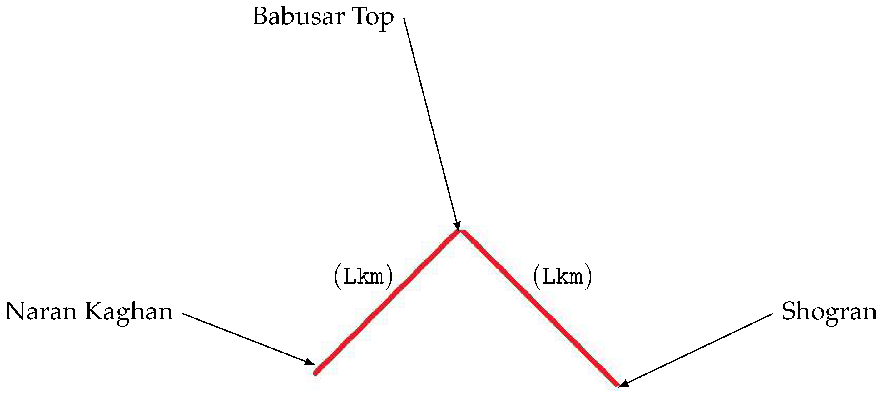
In this example, we demonstrate how harmonic mean and physics dynamics model are related. The problem refers to a university trip to some hilly regions of Pakistan to be organized by Government College University Lahore, which will include visits to Naran Kaghan, Babusar Top, and Shogran.

As shown in Figure 1, there is a track from Naran Kaghan to Shogran. In the absence of land sliding, drivers are likely to travel from Naran Kaghan to Babusar Top at a distance of ($\mathtt{L}\mathtt{km}$) at a pace of (${\mathtt{S}}_{\mathtt{1}}\mathtt{km}/\mathtt{h}$) and to depart from Babusar Top to Shogran at the same distance as Naran Kaghan to Babusar Top but with a speed of (${\mathtt{S}}_{\mathtt{2}}\mathtt{km}/\mathtt{h}$). Therefore, the mean speed of a driver from point Naran Kaghan to Shogran may be determined using the harmonic mean and equals $\mathtt{H}\left({\mathtt{S}}_{\mathtt{1}},{\mathtt{S}}_{\mathtt{2}}\right)\mathtt{km}/\mathtt{h}$ on typical days when there is no land sliding. In case of rainy days or some minor land sliding, the authority instructed tourists to slow down their vehicles by $\mathsf{\alpha }\mathtt{km}/\mathtt{h}$ where $\left(0\le \mathsf{\alpha }\le min\left\{{\mathtt{S}}_{\mathtt{1}},{\mathtt{S}}_{\mathtt{2}}\right\}\right)$. As a result, tourists are permitted to go from Naran Kaghan to Shogran at an average vehicle speed of $\mathtt{H}\left({\mathtt{S}}_{\mathtt{1}},{\mathtt{S}}_{\mathtt{2}}\right)-\mathsf{\alpha }\mathtt{km}/\mathtt{h}$ when the weather conditions are not good.

However, drivers wrongly travel the distance from Naran Kaghan to Babusar Top at ${\mathtt{S}}_{\mathtt{1}}-\mathsf{\alpha }\mathtt{km}/\mathtt{h}$ and the distance from Babusar Top to Shogran at ${\mathtt{S}}_{\mathtt{2}}-\mathsf{\alpha }\mathtt{km}/\mathtt{h}$. As a result, the average speed can be calculated as follows:

$$\mathtt{H}\left({\mathtt{S}}_{\mathtt{1}}-\mathsf{\alpha },{\mathtt{S}}_{\mathtt{2}}-\mathsf{\alpha }\right)={\mathtt{H}}_{\mathsf{\alpha }}\left({\mathtt{S}}_{\mathtt{1}},{\mathtt{S}}_{\mathtt{2}}\right)-\mathsf{\alpha }\mathtt{km}/\mathtt{h}.$$

When the weather conditions are not more reliable, all drivers travel the distance from Naran Kaghan to Shogran at an average speed of

$$\mathtt{H}\left({\mathtt{S}}_{\mathtt{1}},{\mathtt{S}}_{\mathtt{2}}\right)-\mathsf{\alpha }-\mathtt{H}\left({\mathtt{S}}_{\mathtt{1}}-\mathsf{\alpha },{\mathtt{S}}_{\mathtt{2}}-\mathsf{\alpha }\right)=\mathtt{H}\left({\mathtt{S}}_{\mathtt{1}},{\mathtt{S}}_{\mathtt{2}}\right)-{\mathtt{H}}_{\mathsf{\alpha }}\left({\mathtt{S}}_{\mathtt{1}},{\mathtt{S}}_{\mathtt{2}}\right)\mathtt{km}/\mathtt{h}.$$

In this instance, the following formula may be used to determine how long it takes to go from Naran Kaghan to Shogran:

$$\mathtt{t}={\displaystyle \frac{2\mathtt{L}}{\mathtt{H}\left({\mathtt{S}}_{\mathtt{1}},{\mathtt{S}}_{\mathtt{2}}\right)-{\mathtt{H}}_{\mathsf{\alpha }}\left({\mathtt{S}}_{\mathtt{1}},{\mathtt{S}}_{\mathtt{2}}\right)}}\mathtt{h}$$

It is evident from the above that $\mathtt{H}\left({\mathtt{S}}_{\mathtt{1}},{\mathtt{S}}_{\mathtt{2}}\right)-\mathsf{\alpha }$ and $\mathtt{H}\left({\mathtt{S}}_{\mathtt{1}}-\mathsf{\alpha },{\mathtt{S}}_{\mathtt{2}}-\mathsf{\alpha }\right)$ are not same. To reduce the mean speed by factor $\mathsf{\alpha }\mathtt{km}$ $\left(0<\mathsf{\alpha }<min\left\{{\mathtt{S}}_{\mathtt{1}},{\mathtt{S}}_{\mathtt{2}}\right\}\right)$, many drivers likely to cover the distance from Naran Kaghan to Babusar Top at a pace of ${\mathtt{S}}_{\mathtt{1}}-{\mathtt{x}}_{\mathtt{0}}\mathtt{km}/\mathtt{h}$ and from Babusar Top to Shogran at a pace of ${\mathtt{S}}_{\mathtt{2}}-{\mathtt{x}}_{\mathtt{0}}\mathtt{km}/\mathtt{h}$ for some ${\mathtt{x}}_{\mathtt{0}}\left(0<{\mathtt{x}}_{\mathtt{0}}<min\left\{{\mathtt{S}}_{\mathtt{1}},{\mathtt{S}}_{\mathtt{2}}\right\}\right)$. Therefore, one has

$$\begin{array}{cc}& \left|\mathtt{H}\left({\mathtt{S}}_{\mathtt{1}},{\mathtt{S}}_{\mathtt{2}}\right)-\mathsf{\alpha }-\mathtt{H}\left({\mathtt{S}}_{\mathtt{1}}-{\mathtt{x}}_{\mathtt{0}},{\mathtt{S}}_{\mathtt{2}}-{\mathtt{x}}_{\mathtt{0}}\right)\right|\hfill \\ & =\underset{0<\mathtt{x}<min\left\{{\mathtt{S}}_{\mathtt{1}},{\mathtt{S}}_{\mathtt{2}}\right\}}{inf}\left\{\left|\mathtt{H}\left({\mathtt{S}}_{\mathtt{1}},{\mathtt{S}}_{\mathtt{2}}\right)-\mathsf{\alpha }-\mathtt{H}\left({\mathtt{S}}_{\mathtt{1}}-\mathtt{x},{\mathtt{S}}_{\mathtt{2}}-\mathtt{x}\right)\right|\right\}\hfill \\ & =\underset{0<\mathtt{x}<min\left\{{\mathtt{S}}_{\mathtt{1}},{\mathtt{S}}_{\mathtt{2}}\right\}}{inf}\left\{\left|\mathtt{H}\left({\mathtt{S}}_{\mathtt{1}},{\mathtt{S}}_{\mathtt{2}}\right)-{\mathtt{H}}_{\mathtt{x}}\left({\mathtt{S}}_{\mathtt{1}},{\mathtt{S}}_{\mathtt{2}}\right)+\mathtt{x}-\mathsf{\alpha }\right|\right\}\hfill \end{array}$$

It can be easily seen that

$$\begin{array}{cc}\hfill & \underset{0<\mathtt{x}<min\left\{{\mathtt{S}}_{\mathtt{1}},{\mathtt{S}}_{\mathtt{2}}\right\}}{inf}\left\{\left|\mathtt{H}\left({\mathtt{S}}_{\mathtt{1}},{\mathtt{S}}_{\mathtt{2}}\right)-{\mathtt{H}}_{\mathtt{x}}\left({\mathtt{S}}_{\mathtt{1}},{\mathtt{S}}_{\mathtt{2}}\right)+\mathtt{x}-\mathsf{\alpha }\right|\right\}\hfill \\ \hfill & \underset{0<\mathtt{x}<min\left\{{\mathtt{S}}_{\mathtt{1}},{\mathtt{S}}_{\mathtt{2}}\right\}}{inf}\left\{2\left({\mathtt{S}}_{\mathtt{1}}+{\mathtt{S}}_{\mathtt{2}}\right){\mathtt{x}}^2-\left(2{\mathtt{S}}_{\mathtt{1}}^2+2{\mathtt{S}}_{\mathtt{2}}^2+2\mathsf{\vartheta }\left({\mathtt{S}}_{\mathtt{1}}+{\mathtt{S}}_{\mathtt{2}}\right)\right)x+{\left({\mathtt{S}}_{\mathtt{1}}+{\mathtt{S}}_{\mathtt{2}}\right)}^2\right.\hfill \\ \hfill & =0\}\hfill \\ \hfill & =0\hfill \end{array}$$

(1)

and is obtained at point

$$\begin{array}{c}\hfill {\mathtt{x}}_{\mathtt{0}}={\displaystyle \frac{{\mathtt{S}}_{\mathtt{1}}^2+{\mathtt{S}}_{\mathtt{2}}^2+\mathsf{\vartheta }\left({\mathtt{S}}_{\mathtt{1}}+{\mathtt{S}}_{\mathtt{2}}\right)-\sqrt{{\delta }_{\mathsf{\alpha }}\left({\mathtt{S}}_{\mathtt{1}},{\mathtt{S}}_{\mathtt{2}}\right)}}{2\left({\mathtt{S}}_{\mathtt{1}}+{\mathtt{S}}_{\mathtt{2}}\right)}}.\end{array}$$

(2)

where

$${\delta }_{\mathsf{\alpha }}\left({\mathtt{S}}_{\mathtt{1}},{\mathtt{S}}_{\mathtt{2}}\right):={\left({\mathtt{S}}_{\mathtt{1}}^2-\mathsf{\alpha }{\mathtt{S}}_{\mathtt{2}}\right)}^2+{\left({\mathtt{S}}_{\mathtt{2}}^2-\mathsf{\alpha }{\mathtt{S}}_{\mathtt{1}}\right)}^2+2{\mathtt{S}}_{\mathtt{1}}{\mathtt{S}}_{\mathtt{2}}\left({\mathtt{S}}_{\mathtt{1}}-\mathsf{\alpha }\right)\left({\mathtt{S}}_{\mathtt{2}}-\mathsf{\alpha }\right)$$

Example 1. 

Assume that the driver accelerates to $25\mathtt{km}/\mathtt{h}$ as they go from Naran Kaghan to Babusar Top and at the rate of $70\mathtt{km}/\mathtt{h}$ from Babusar Top to Shogran for the distance from Naran Kaghan to Shogran (see Figure 1). Consequently, their average speed as they go from Naran Kaghan to Shogran is $\mathtt{H}(25,70)=37\mathtt{km}/\mathtt{h}$. By (2) we have ${\mathtt{x}}_{\mathtt{0}}=4.9$.

Hence, if a driver decreases his speed from Naran Kaghan to Shogran with the average speed of factor $\mathsf{\alpha }=5\mathtt{km}/\mathtt{h}$, by (2) he will be able to travel from Naran Kaghan to Babusar Top at $25-4.9=20.1\mathtt{km}/\mathtt{h}$ and from Babusar Top to Shogran at $75-4.9=70.1\mathtt{km}/\mathtt{h}$.

2.2. Some Fractional Identities

In this section, we use the following definition of Riemann–Liouville fractional ($\mathtt{RLF}$) integral to develop some fractional identities that we use in several main results for Milne-type inequalities.

Definition 7 

(See [63]). Let $\mathsf{\theta }:[{\mathsf{\mu }}_1,{\mathsf{\mu }}_2]\to \mathsf{R}$ be Lebesgue integrable continuous function on $[{\mathsf{\mu }}_1,{\mathsf{\mu }}_2]$. The $\mathtt{RLF}$ integrals are defined for $\mathsf{\alpha }>0$ by

$${\mathsf{J}}_{{\mathsf{\mu }}_1+}^{\mathsf{\alpha }}\mathsf{\theta }\left(x\right)={\displaystyle \frac{1}{\Gamma \left(\mathsf{\alpha }\right)}}{\int }_{{\mathsf{\mu }}_1}^x{(x-\mathsf{\nu })}^{\mathsf{\alpha }-1}\mathsf{\theta }(\mathsf{\nu })\mathtt{d}\mathsf{\nu }$$

for ${\mathsf{\mu }}_1<x⩽{\mathsf{\mu }}_2$ and

$${\mathsf{J}}_{{\mathsf{\mu }}_2-}^{\mathsf{\alpha }}\mathsf{\theta }\left(x\right)={\displaystyle \frac{1}{\Gamma \left(\mathsf{\alpha }\right)}}{\int }_{\mathtt{x}}^{{\mathsf{\mu }}_2}{(\mathsf{\nu }-x)}^{\mathsf{\alpha }-1}\mathsf{\theta }(\mathsf{\nu })\mathtt{d}\mathsf{\nu }$$

for ${\mathsf{\mu }}_1⩽x<{\mathsf{\mu }}_2$, where Γ is the special function.

Lemma 1. 

Let $\mathsf{\theta }:[{\mathsf{\mu }}_1,{\mathsf{\mu }}_2]\to \mathsf{R}$ be an absolutely continuous function on $[{\mathsf{\mu }}_1,{\mathsf{\mu }}_2]$.

• For any $\mathtt{x}\in ({\mathsf{\mu }}_1,{\mathsf{\mu }}_2)$ we have

$$\begin{array}{cc}\hfill & {\mathsf{J}}_{{\mathsf{\mu }}_1+}^{\mathsf{\alpha }}\mathsf{\theta }\left(x\right)+{\mathsf{J}}_{{\mathsf{\mu }}_2-}^{\mathsf{\alpha }}\mathsf{\theta }\left(x\right)\hfill \\ \hfill & ={\displaystyle \frac{1}{\Gamma (\mathsf{\alpha }+1)}}\left[{(x-{\mathsf{\mu }}_1)}^{\mathsf{\alpha }}\mathsf{\theta }\left(\mathtt{G}\right)+{({\mathsf{\mu }}_2-\mathtt{x})}^{\mathsf{\alpha }}\mathsf{\theta }\left(\mathtt{H}\right)\right]\hfill \\ \hfill & +{\displaystyle \frac{1}{\Gamma (\mathsf{\alpha }+1)}}\left[{\int }_{{\mathsf{\mu }}_1}^x{(x-\mathsf{\nu })}^{\mathsf{\alpha }}{\mathsf{\theta }}^{\prime }(\mathsf{\nu })\mathtt{d}\mathsf{\nu }-{\int }_{\mathtt{x}}^{{\mathsf{\mu }}_2}{(\mathsf{\nu }-\mathtt{x})}^{\mathsf{\alpha }}{\mathsf{\theta }}^{\prime }(\mathsf{\nu })\mathtt{d}\mathsf{\nu }\right].\hfill \end{array}$$

(3)

Proof. 

Since $\mathsf{\theta }:[{\mathsf{\mu }}_1,{\mathsf{\mu }}_2]\to \mathsf{R}$ be an absolutely continuous function on $[{\mathsf{\mu }}_1,{\mathsf{\mu }}_2]$, then the integrals

$${\int }_{{\mathsf{\mu }}_1}^x{(x-\mathsf{\nu })}^{\mathsf{\alpha }}{\mathsf{\theta }}^{\prime }(\mathsf{\nu })\mathtt{d}\mathsf{\nu }\mathrm{and}{\int }_{\mathtt{x}}^{{\mathsf{\mu }}_2}{(\mathsf{\nu }-\mathtt{x})}^{\mathsf{\alpha }}{\mathsf{\theta }}^{\prime }(\mathsf{\nu })\mathtt{d}\mathsf{\nu }$$

exist and integrating by parts, we have

$$\begin{array}{cc}\hfill & {\displaystyle \frac{1}{\Gamma (\mathsf{\alpha }+1)}}{\int }_{{\mathsf{\mu }}_1}^x{(x-\mathsf{\nu })}^{\mathsf{\alpha }}{\mathsf{\theta }}^{\prime }(\mathsf{\nu })\mathtt{d}\mathsf{\nu }\hfill \\ \hfill & ={\displaystyle \frac{1}{\Gamma \left(\mathsf{\alpha }\right)}}{\int }_{{\mathsf{\mu }}_1}^x{(x-\mathsf{\nu })}^{\mathsf{\alpha }-1}\mathsf{\theta }(\mathsf{\nu })\mathtt{d}\mathsf{\nu }-{\displaystyle \frac{1}{\Gamma (\mathsf{\alpha }+1)}}{(x-{\mathsf{\mu }}_1)}^{\mathsf{\alpha }}\mathsf{\theta }\left({\mathsf{\mu }}_1\right)\hfill \\ \hfill & ={\mathsf{J}}_{{\mathsf{\mu }}_1+}^{\mathsf{\alpha }}\mathsf{\theta }\left(x\right)-{\displaystyle \frac{1}{\Gamma (\mathsf{\alpha }+1)}}{(x-{\mathsf{\mu }}_1)}^{\mathsf{\alpha }}\mathsf{\theta }\left({\mathsf{\mu }}_1\right)\hfill \end{array}$$

(4)

for ${\mathsf{\mu }}_1<x⩽{\mathsf{\mu }}_2$ and

$$\begin{array}{cc}\hfill & {\displaystyle \frac{1}{\Gamma (\mathsf{\alpha }+1)}}{\int }_{\mathtt{x}}^{{\mathsf{\mu }}_2}{(\mathsf{\nu }-\mathtt{x})}^{\mathsf{\alpha }}{\mathsf{\theta }}^{\prime }(\mathsf{\nu })\mathtt{d}\mathsf{\nu }\hfill \\ \hfill & ={\displaystyle \frac{1}{\Gamma (\mathsf{\alpha }+1)}}{({\mathsf{\mu }}_2-\mathtt{x})}^{\mathsf{\alpha }}\mathsf{\theta }\left({\mathsf{\mu }}_2\right)-{\displaystyle \frac{1}{\Gamma \left(\mathsf{\alpha }\right)}}{\int }_{\mathtt{x}}^{{\mathsf{\mu }}_2}{(\mathsf{\nu }-\mathtt{x})}^{\mathsf{\alpha }-1}\mathsf{\theta }(\mathsf{\nu })\mathtt{d}\mathsf{\nu }\hfill \\ \hfill & ={\displaystyle \frac{1}{\Gamma (\mathsf{\alpha }+1)}}{({\mathsf{\mu }}_2-\mathtt{x})}^{\mathsf{\alpha }}\mathsf{\theta }\left({\mathsf{\mu }}_2\right)-{\mathsf{J}}_{{\mathsf{\mu }}_2-}^{\mathsf{\alpha }}\mathsf{\theta }\left(x\right)\hfill \end{array}$$

(5)

for ${\mathsf{\mu }}_1⩽\mathtt{x}<{\mathsf{\mu }}_2$. From (4) we have

$${\mathsf{J}}_{{\mathsf{\mu }}_1+}^{\mathsf{\alpha }}\mathsf{\theta }\left(x\right)={\displaystyle \frac{1}{\Gamma (\mathsf{\alpha }+1)}}{(x-{\mathsf{\mu }}_1)}^{\mathsf{\alpha }}\mathsf{\theta }\left({\mathsf{\mu }}_1\right)+{\displaystyle \frac{1}{\Gamma (\mathsf{\alpha }+1)}}{\int }_{{\mathsf{\mu }}_1}^x{(x-\mathsf{\nu })}^{\mathsf{\alpha }}{\mathsf{\theta }}^{\prime }(\mathsf{\nu })\mathtt{d}\mathsf{\nu }$$

for ${\mathsf{\mu }}_1<x⩽{\mathsf{\mu }}_2$ and from (5) we have

$${\mathsf{J}}_{{\mathsf{\mu }}_2-}^{\mathsf{\alpha }}\mathsf{\theta }\left(x\right)={\displaystyle \frac{1}{\Gamma (\mathsf{\alpha }+1)}}{({\mathsf{\mu }}_2-\mathtt{x})}^{\mathsf{\alpha }}\mathsf{\theta }\left({\mathsf{\mu }}_2\right)-{\displaystyle \frac{1}{\Gamma (\mathsf{\alpha }+1)}}{\int }_{\mathtt{x}}^{{\mathsf{\mu }}_2}{(\mathsf{\nu }-\mathtt{x})}^{\mathsf{\alpha }}{\mathsf{\theta }}^{\prime }(\mathsf{\nu })\mathtt{d}\mathsf{\nu }.$$

□

Lemma 2. 

Let $\mathsf{\theta }:[{\mathsf{\mu }}_1,{\mathsf{\mu }}_2]\to \mathsf{R}$ be an absolutely continuous function on $[{\mathsf{\mu }}_1,{\mathsf{\mu }}_2]$.

• For any $x\in ({\mathsf{\mu }}_1,{\mathsf{\mu }}_2)$ we have

  $$\begin{array}{cc}& {\mathsf{J}}_{x-}^{\mathsf{\alpha }}\mathsf{\theta }\left({\mathsf{\mu }}_1\right)+{\mathsf{J}}_{x+}^{\mathsf{\alpha }}\mathsf{\theta }\left({\mathsf{\mu }}_2\right)\hfill \\ & ={\displaystyle \frac{1}{\Gamma (\mathsf{\alpha }+1)}}\left[{(x-{\mathsf{\mu }}_1)}^{\mathsf{\alpha }}+{({\mathsf{\mu }}_2-\mathtt{x})}^{\mathsf{\alpha }}\right]\mathsf{\theta }\left(x\right)\hfill \\ & +{\displaystyle \frac{1}{\Gamma (\mathsf{\alpha }+1)}}\left[{\int }_{\mathtt{x}}^{{\mathsf{\mu }}_2}{({\mathsf{\mu }}_2-\mathsf{\nu })}^{\mathsf{\alpha }}{\mathsf{\theta }}^{\prime }(\mathsf{\nu })\mathtt{d}\mathsf{\nu }-{\int }_{{\mathsf{\mu }}_1}^x{(\mathsf{\nu }-{\mathsf{\mu }}_1)}^{\mathsf{\alpha }}{\mathsf{\theta }}^{\prime }(\mathsf{\nu })\mathtt{d}\mathsf{\nu }\right].\hfill \end{array}$$

Proof. 

Since we have

$${\mathsf{J}}_{x+}^{\mathsf{\alpha }}\mathsf{\theta }\left({\mathsf{\mu }}_2\right)={\displaystyle \frac{1}{\Gamma \left(\mathsf{\alpha }\right)}}{\int }_{\mathtt{x}}^{{\mathsf{\mu }}_2}{({\mathsf{\mu }}_2-\mathsf{\nu })}^{\mathsf{\alpha }-1}\mathsf{\theta }(\mathsf{\nu })\mathtt{d}\mathsf{\nu }$$

for ${\mathsf{\mu }}_1⩽\mathtt{x}<{\mathsf{\mu }}_2$ and

$${\mathsf{J}}_{x-}^{\mathsf{\alpha }}\mathsf{\theta }\left({\mathsf{\mu }}_1\right)={\displaystyle \frac{1}{\Gamma \left(\mathsf{\alpha }\right)}}{\int }_{{\mathsf{\mu }}_1}^x{(\mathsf{\nu }-{\mathsf{\mu }}_1)}^{\mathsf{\alpha }-1}\mathsf{\theta }(\mathsf{\nu })\mathtt{d}\mathsf{\nu }$$

for ${\mathsf{\mu }}_1<x⩽{\mathsf{\mu }}_2$. Since $\mathsf{\theta }:[{\mathsf{\mu }}_1,{\mathsf{\mu }}_2]\to \mathsf{R}$ be an absolutely continuous function $[{\mathsf{\mu }}_1,{\mathsf{\mu }}_2]$, then the integrals

$${\int }_{{\mathsf{\mu }}_1}^x{(\mathsf{\nu }-{\mathsf{\mu }}_1)}^{\mathsf{\alpha }}{\mathsf{\theta }}^{\prime }(\mathsf{\nu })\mathtt{d}\mathsf{\nu }\mathrm{and}{\int }_{\mathtt{x}}^{{\mathsf{\mu }}_2}{({\mathsf{\mu }}_2-\mathsf{\nu })}^{\mathsf{\alpha }}{\mathsf{\theta }}^{\prime }(\mathsf{\nu })\mathtt{d}\mathsf{\nu }$$

exist and integrating by parts, we have

$$\begin{array}{cc}\hfill & {\displaystyle \frac{1}{\Gamma (\mathsf{\alpha }+1)}}{\int }_{{\mathsf{\mu }}_1}^x{(\mathsf{\nu }-{\mathsf{\mu }}_1)}^{\mathsf{\alpha }}{\mathsf{\theta }}^{\prime }(\mathsf{\nu })\mathtt{d}\mathsf{\nu }\hfill \\ \hfill & ={\displaystyle \frac{1}{\Gamma (\mathsf{\alpha }+1)}}{(x-{\mathsf{\mu }}_1)}^{\mathsf{\alpha }}\mathsf{\theta }\left(x\right)-{\displaystyle \frac{1}{\Gamma \left(\mathsf{\alpha }\right)}}{\int }_{{\mathsf{\mu }}_1}^x{(\mathsf{\nu }-{\mathsf{\mu }}_1)}^{\mathsf{\alpha }-1}\mathsf{\theta }(\mathsf{\nu })\mathtt{d}\mathsf{\nu }\hfill \\ \hfill & ={\displaystyle \frac{1}{\Gamma (\mathsf{\alpha }+1)}}{(x-{\mathsf{\mu }}_1)}^{\mathsf{\alpha }}\mathsf{\theta }\left(x\right)-{\mathsf{J}}_{x-}^{\mathsf{\alpha }}\mathsf{\theta }\left({\mathsf{\mu }}_1\right)\hfill \end{array}$$

(6)

for ${\mathsf{\mu }}_1<x⩽{\mathsf{\mu }}_2$ and

$$\begin{array}{cc}\hfill & {\displaystyle \frac{1}{\Gamma (\mathsf{\alpha }+1)}}{\int }_{\mathtt{x}}^{{\mathsf{\mu }}_2}{({\mathsf{\mu }}_2-\mathsf{\nu })}^{\mathsf{\alpha }}{\mathsf{\theta }}^{\prime }(\mathsf{\nu })\mathtt{d}\mathsf{\nu }\hfill \\ \hfill & ={\displaystyle \frac{1}{\Gamma \left(\mathsf{\alpha }\right)}}{\int }_{\mathtt{x}}^{{\mathsf{\mu }}_2}{({\mathsf{\mu }}_2-\mathsf{\nu })}^{\mathsf{\alpha }-1}\mathsf{\theta }(\mathsf{\nu })\mathtt{d}\mathsf{\nu }-{\displaystyle \frac{1}{\Gamma (\mathsf{\alpha }+1)}}{({\mathsf{\mu }}_2-\mathtt{x})}^{\mathsf{\alpha }}\mathsf{\theta }\left(x\right)\hfill \\ \hfill & ={\mathsf{J}}_{x+}^{\mathsf{\alpha }}\mathsf{\theta }\left({\mathsf{\mu }}_2\right)-{\displaystyle \frac{1}{\Gamma (\mathsf{\alpha }+1)}}{({\mathsf{\mu }}_2-\mathtt{x})}^{\mathsf{\alpha }}\mathsf{\theta }\left(x\right)\hfill \end{array}$$

(7)

for ${\mathsf{\mu }}_1⩽\mathtt{x}<{\mathsf{\mu }}_2$. From (6) we have

$${\mathsf{J}}_{x-}^{\mathsf{\alpha }}\mathsf{\theta }\left({\mathsf{\mu }}_1\right)={\displaystyle \frac{1}{\Gamma (\mathsf{\alpha }+1)}}{(x-{\mathsf{\mu }}_1)}^{\mathsf{\alpha }}\mathsf{\theta }\left(x\right)-{\displaystyle \frac{1}{\Gamma (\mathsf{\alpha }+1)}}{\int }_{{\mathsf{\mu }}_1}^x{(\mathsf{\nu }-{\mathsf{\mu }}_1)}^{\mathsf{\alpha }}{\mathsf{\theta }}^{\prime }(\mathsf{\nu })\mathtt{d}\mathsf{\nu }$$

for ${\mathsf{\mu }}_1<x⩽{\mathsf{\mu }}_2$ and from (7)

$${\mathsf{J}}_{x+}^{\mathsf{\alpha }}\mathsf{\theta }\left({\mathsf{\mu }}_2\right)={\displaystyle \frac{1}{\Gamma (\mathsf{\alpha }+1)}}{({\mathsf{\mu }}_2-\mathtt{x})}^{\mathsf{\alpha }}\mathsf{\theta }\left(x\right)+{\displaystyle \frac{1}{\Gamma (\mathsf{\alpha }+1)}}{\int }_{\mathtt{x}}^{{\mathsf{\mu }}_2}{({\mathsf{\mu }}_2-\mathsf{\nu })}^{\mathsf{\alpha }}{\mathsf{\theta }}^{\prime }(\mathsf{\nu })\mathtt{d}\mathsf{\nu }.$$

□

Corollary 2. 

Let $\mathsf{\theta }:[{\mathsf{\mu }}_1,{\mathsf{\mu }}_2]\to \mathsf{R}$ be an absolutely continuous function on $[{\mathsf{\mu }}_1,{\mathsf{\mu }}_2]$. We now possess the midpoint equality

$$\begin{array}{cc}& {\mathsf{J}}_{{\mathsf{\mu }}_1+}^{\mathsf{\alpha }}\mathsf{\theta }\left({\displaystyle \frac{{\mathsf{\mu }}_1+{\mathsf{\mu }}_2}{2}}\right)+{\mathsf{J}}_{{\mathsf{\mu }}_2-}^{\mathsf{\alpha }}\mathsf{\theta }\left({\displaystyle \frac{{\mathsf{\mu }}_1+{\mathsf{\mu }}_2}{2}}\right)\hfill \\ & ={\displaystyle \frac{1}{2^{\mathsf{\alpha }-1}\Gamma (\mathsf{\alpha }+1)}}{\displaystyle \frac{\mathsf{\theta }\left({\mathsf{\mu }}_1\right)+\mathsf{\theta }\left({\mathsf{\mu }}_2\right)}{2}}\hfill \\ & +{\displaystyle \frac{1}{\Gamma (\mathsf{\alpha }+1)}}\left[{\int }_{{\mathsf{\mu }}_1}^{{\displaystyle \frac{{\mathsf{\mu }}_1+{\mathsf{\mu }}_2}{2}}}{\left({\displaystyle \frac{{\mathsf{\mu }}_1+{\mathsf{\mu }}_2}{2}}-\mathsf{\nu }\right)}^{\mathsf{\alpha }}{\mathsf{\theta }}^{\prime }(\mathsf{\nu })\mathtt{d}\mathsf{\nu }-{\int }_{{\displaystyle \frac{{\mathsf{\mu }}_1+{\mathsf{\mu }}_2}{2}}}^{{\mathsf{\mu }}_2}{\left(\mathsf{\nu }-{\displaystyle \frac{{\mathsf{\mu }}_1+{\mathsf{\mu }}_2}{2}}\right)}^{\mathsf{\alpha }}{\mathsf{\theta }}^{\prime }(\mathsf{\nu })\mathtt{d}\mathsf{\nu }\right]\hfill \end{array}$$

and

$$\begin{array}{cc}\hfill & {\mathsf{J}}_{{\displaystyle \frac{{\mathsf{\mu }}_1+{\mathsf{\mu }}_2}{2}}-}^{\mathsf{\alpha }}\mathsf{\theta }\left({\mathsf{\mu }}_1\right)+{\mathsf{J}}_{{\displaystyle \frac{{\mathsf{\mu }}_1+{\mathsf{\mu }}_2}{2}}+}^{\mathsf{\alpha }}\mathsf{\theta }\left({\mathsf{\mu }}_2\right)\hfill \\ \hfill & ={\displaystyle \frac{1}{2^{\mathsf{\alpha }-1}\Gamma (\mathsf{\alpha }+1)}}\mathsf{\theta }\left({\displaystyle \frac{{\mathsf{\mu }}_1+{\mathsf{\mu }}_2}{2}}\right){({\mathsf{\mu }}_2-{\mathsf{\mu }}_1)}^{\mathsf{\alpha }}\hfill \\ \hfill & +{\displaystyle \frac{1}{\Gamma (\mathsf{\alpha }+1)}}\left[{\int }_{{\displaystyle \frac{{\mathsf{\mu }}_1+{\mathsf{\mu }}_2}{2}}}^{{\mathsf{\mu }}_2}{({\mathsf{\mu }}_2-\mathsf{\nu })}^{\mathsf{\alpha }}{\mathsf{\theta }}^{\prime }(\mathsf{\nu })\mathtt{d}\mathsf{\nu }-{\int }_{{\mathsf{\mu }}_1}^{{\displaystyle \frac{{\mathsf{\mu }}_1+{\mathsf{\mu }}_2}{2}}}{(\mathsf{\nu }-{\mathsf{\mu }}_1)}^{\mathsf{\alpha }}{\mathsf{\theta }}^{\prime }(\mathsf{\nu })\mathtt{d}\mathsf{\nu }\right],\hfill \end{array}$$

(8)

for ${\mathsf{\mu }}_1⩽{\displaystyle \frac{{\mathsf{\mu }}_1+{\mathsf{\mu }}_2}{2}}<{\mathsf{\mu }}_2$. From (8) we have

$$\begin{array}{cc}\hfill & {\mathsf{J}}_{{\displaystyle \frac{{\mathsf{\mu }}_1+{\mathsf{\mu }}_2}{2}}-}^{\mathsf{\alpha }}\mathsf{\theta }\left({\mathsf{\mu }}_1\right)={\displaystyle \frac{1}{2^{\mathsf{\alpha }-1}\Gamma (\mathsf{\alpha }+1)}}\mathsf{\theta }\left({\displaystyle \frac{{\mathsf{\mu }}_1+{\mathsf{\mu }}_2}{2}}\right){({\mathsf{\mu }}_2-{\mathsf{\mu }}_1)}^{\mathsf{\alpha }}-{\displaystyle \frac{1}{\Gamma (\mathsf{\alpha }+1)}}\left[{\int }_{{\mathsf{\mu }}_1}^{{\displaystyle \frac{{\mathsf{\mu }}_1+{\mathsf{\mu }}_2}{2}}}{(\mathsf{\nu }-{\mathsf{\mu }}_1)}^{\mathsf{\alpha }}{\mathsf{\theta }}^{\prime }(\mathsf{\nu })\mathtt{d}\mathsf{\nu }\right]\hfill \\ & ={\displaystyle \frac{1}{2^{\mathsf{\alpha }-1}\Gamma (\mathsf{\alpha }+1)}}\mathsf{\theta }\left({\displaystyle \frac{{\mathsf{\mu }}_1+{\mathsf{\mu }}_2}{2}}\right){({\mathsf{\mu }}_2-{\mathsf{\mu }}_1)}^{\mathsf{\alpha }}-{\displaystyle \frac{{\mathsf{\delta }}^{\mathsf{\alpha }}{({\mathsf{\mu }}_2-{\mathsf{\mu }}_1)}^{\mathsf{\alpha }+1}}{2^{\mathsf{\alpha }+1}\Gamma (\mathsf{\alpha }+1)}}\left[{\int }_0^1{\mathsf{\theta }}^{\prime }\left((1-\mathsf{\delta }){\mathsf{\mu }}_1+\left({\displaystyle \frac{{\mathsf{\mu }}_1+{\mathsf{\mu }}_2}{2}}\right)\mathsf{\delta }\right)\mathtt{d}\mathsf{\delta }\right],\hfill \end{array}$$

(9)

for ${\mathsf{\mu }}_1<{\displaystyle \frac{{\mathsf{\mu }}_1+{\mathsf{\mu }}_2}{2}}⩽{\mathsf{\mu }}_2$ and from (8) we have

$$\begin{array}{cc}\hfill & {\mathsf{J}}_{{\displaystyle \frac{{\mathsf{\mu }}_1+{\mathsf{\mu }}_2}{2}}+}^{\mathsf{\alpha }}\mathsf{\theta }\left({\mathsf{\mu }}_2\right)={\displaystyle \frac{1}{2^{\mathsf{\alpha }-1}\Gamma (\mathsf{\alpha }+1)}}\mathsf{\theta }\left({\displaystyle \frac{{\mathsf{\mu }}_1+{\mathsf{\mu }}_2}{2}}\right){({\mathsf{\mu }}_2-{\mathsf{\mu }}_1)}^{\mathsf{\alpha }}+{\displaystyle \frac{1}{\Gamma (\mathsf{\alpha }+1)}}\left[{\int }_{{\displaystyle \frac{{\mathsf{\mu }}_1+{\mathsf{\mu }}_2}{2}}}^{{\mathsf{\mu }}_2}{({\mathsf{\mu }}_2-\mathsf{\nu })}^{\mathsf{\alpha }}{\mathsf{\theta }}^{\prime }(\mathsf{\nu })\mathtt{d}\mathsf{\nu }\right]\hfill \\ & ={\displaystyle \frac{1}{2^{\mathsf{\alpha }-1}\Gamma (\mathsf{\alpha }+1)}}\mathsf{\theta }\left({\displaystyle \frac{{\mathsf{\mu }}_1+{\mathsf{\mu }}_2}{2}}\right){({\mathsf{\mu }}_2-{\mathsf{\mu }}_1)}^{\mathsf{\alpha }}-{\displaystyle \frac{{(1-\mathsf{\delta })}^{\mathsf{\alpha }}{({\mathsf{\mu }}_2-{\mathsf{\mu }}_1)}^{\mathsf{\alpha }+1}}{2^{\mathsf{\alpha }+1}\Gamma (\mathsf{\alpha }+1)}}\left[{\int }_0^1{\mathsf{\theta }}^{\prime }\left((1-\mathsf{\delta })\left({\displaystyle \frac{{\mathsf{\mu }}_1+{\mathsf{\mu }}_2}{2}}\right)+{\mathsf{\mu }}_2\mathsf{\delta }\right)\mathtt{d}\mathsf{\delta }\right].\hfill \end{array}$$

(10)

3. Main Results

Based on some relational properties and arithmetic operations of tensor analysis, we can extend classical harmonic convex mappings in the operator sense by utilizing the spectrum of a self-adjoint operator in a Hilbert space.

Definition 8. 

$\mathtt{G}$ and $\mathtt{H}$ are selfadjoint operators with $\mathtt{Sp}\left(\mathtt{G}\right),\mathtt{Sp}\left(\mathtt{H}\right)\subset \mathsf{\Omega }$. Assume that $\mathsf{\theta }$ is a continuous and harmonically convex (concave) function on Ω, then for all $\mathsf{\nu }\in [0,1],$ one has

$$\mathsf{\theta }\left({\displaystyle \frac{A\otimes 1\otimes \mathtt{H}\otimes 1}{(1-\mathsf{\nu })\mathtt{G}\otimes 1+\mathsf{\nu }1\otimes \mathtt{H}}}\right)\le (\ge )(1-\mathsf{\nu })\mathsf{\theta }\left(\mathtt{G}\right)\otimes 1+\mathsf{\nu }1\otimes \mathsf{\theta }\left(\mathtt{H}\right).$$

Our main findings are based on the following representation results derived using various arithmetic operations for continuous functions:

Lemma 3. 

Let $\mathtt{G}$ and $\mathtt{H}$ be selfadjoint operators with $\mathtt{Sp}\left(\mathtt{G}\right)\subset {\mathsf{\Omega }}_1$ and $\mathtt{Sp}\left(\mathtt{H}\right)\subset$ ${\mathsf{\Omega }}_2$. Assume $\mathsf{\theta },\mathsf{\psi }$ be continuous on ${\mathsf{\Omega }}_1$ and $\Phi ,\mathsf{\vartheta }$ continuous on ${\mathsf{\Omega }}_2$ and $\mathsf{\phi }$ continuous on Ω it comprises the sum of the intervals $\mathsf{\psi }\left({\mathsf{\Omega }}_1\right)+\mathsf{\vartheta }\left({\mathsf{\Omega }}_2\right)$, then one has

$$\begin{array}{cc}\hfill & \left(\mathsf{\theta }\right(\mathtt{G})\otimes 1+1\otimes \Phi (\mathtt{H}\left)\right)\mathsf{\phi }\left(\mathsf{\psi }\right(\mathtt{G})\otimes 1+1\otimes \mathsf{\vartheta }(\mathtt{H}\left)\right)\hfill \\ \hfill & ={\int }_{{\mathsf{\Omega }}_1}{\int }_{{\mathsf{\Omega }}_2}(\mathsf{\theta }\left({\mathsf{\mu }}_2\right)+\Phi \left({\mathsf{\mu }}_1\right))\mathsf{\phi }(\mathsf{\psi }\left({\mathsf{\mu }}_2\right)+\mathsf{\vartheta }\left({\mathsf{\mu }}_1\right))\mathtt{d}{\mathtt{E}}_{{\mathsf{\Omega }}_1}\otimes {\mathtt{dF}}_{{\mathsf{\Omega }}_2},\hfill \end{array}$$

(11)

where $\mathtt{G}$ and $\mathtt{H}$ have the spectral resolutions

$$\mathtt{G}={\int }_{{\mathsf{\Omega }}_1}{\mathsf{\mu }}_2\mathtt{dE}\left({\mathsf{\mu }}_2\right)\mathrm{and}\mathtt{H}={\int }_{{\mathsf{\Omega }}_2}{\mathsf{\mu }}_1\mathtt{dF}\left({\mathsf{\mu }}_1\right).$$

Proof. 

A polynomial sequence can be used to approximate any continuous function, according to Stone–Weierstrass; hence, confirming the exponential function’s equality is sufficient. Consider $\mathsf{\phi }\left(\mathsf{\mu }\right)=e^{{\mathsf{\mu }}^{\mathtt{n}}}$ with $\mathtt{n}$ is any natural number, then we have

$$\begin{array}{cc}\hfill \mathcal{F}& :={\int }_{{\mathsf{\Omega }}_1}{\int }_{{\mathsf{\Omega }}_2}(\mathsf{\theta }\left({\mathsf{\mu }}_2\right)+\Phi \left({\mathsf{\mu }}_1\right))e^{{(\mathsf{\psi }\left({\mathsf{\mu }}_2\right)+\mathsf{\vartheta }\left({\mathsf{\mu }}_1\right))}^{\mathtt{n}}}\mathtt{d}{\mathtt{E}}_{{\mathsf{\Omega }}_1}\otimes {\mathtt{dF}}_{{\mathsf{\Omega }}_2}\hfill \\ & ={\int }_{{\mathsf{\Omega }}_1}{\int }_{{\mathsf{\Omega }}_2}(\mathsf{\theta }\left({\mathsf{\mu }}_2\right)+\Phi \left({\mathsf{\mu }}_1\right))\sum _{\mathtt{m}=\mathtt{0}}^{\mathtt{n}}{C}_{\mathtt{n}}^{\mathtt{m}}{e}^{{\left[\mathsf{\psi }\left({\mathsf{\mu }}_2\right)\right]}^{\mathtt{m}}}{e}^{{\left[\mathsf{\vartheta }\left({\mathsf{\mu }}_1\right)\right]}^{\mathtt{n}-\mathtt{m}}}\mathtt{d}{\mathtt{E}}_{{\mathsf{\Omega }}_1}\otimes {\mathtt{dF}}_{{\mathsf{\Omega }}_2}\hfill \\ & =\sum _{\mathtt{m}=\mathtt{0}}^{\mathtt{n}}{C}_{\mathtt{n}}^{\mathtt{m}}{\int }_{{\mathsf{\Omega }}_1}{\int }_{{\mathsf{\Omega }}_2}(\mathsf{\theta }\left({\mathsf{\mu }}_2\right)+\Phi \left({\mathsf{\mu }}_1\right))e^{{\left[\mathsf{\psi }\left({\mathsf{\mu }}_2\right)\right]}^{\mathtt{m}}}{e}^{{\left[\mathsf{\vartheta }\left({\mathsf{\mu }}_1\right)\right]}^{\mathtt{n}-\mathtt{m}}}\mathtt{d}{\mathtt{E}}_{{\mathsf{\Omega }}_1}\otimes {\mathtt{dF}}_{{\mathsf{\Omega }}_2}\hfill \\ & =\sum _{\mathtt{m}=\mathtt{0}}^{\mathtt{n}}{C}_{\mathtt{n}}^{\mathtt{m}}\left[{\int }_{{\mathsf{\Omega }}_1}{\int }_{{\mathsf{\Omega }}_2}\mathsf{\theta }\left({\mathsf{\mu }}_2\right)e^{{\left[\mathsf{\psi }\left({\mathsf{\mu }}_2\right)\right]}^{\mathtt{m}}}{e}^{{\left[\mathsf{\vartheta }\left({\mathsf{\mu }}_1\right)\right]}^{\mathtt{n}-\mathtt{m}}}\mathtt{d}{\mathtt{E}}_{{\mathsf{\Omega }}_1}\otimes {\mathtt{dF}}_{{\mathsf{\Omega }}_2}\right.\hfill \\ & \left.+{\int }_{{\mathsf{\Omega }}_1}{\int }_{{\mathsf{\Omega }}_2}{e}^{{\left[\mathsf{\psi }\left({\mathsf{\mu }}_2\right)\right]}^{\mathtt{m}}}\Phi \left({\mathsf{\mu }}_1\right)e^{{\left[\mathsf{\vartheta }\left({\mathsf{\mu }}_1\right)\right]}^{\mathtt{n}-\mathtt{m}}}\mathtt{d}{\mathtt{E}}_{{\mathsf{\Omega }}_1}\otimes {\mathtt{dF}}_{{\mathsf{\Omega }}_2}\right].\hfill \end{array}$$

Observe that

$$\begin{array}{cc}& {\int }_{{\mathsf{\Omega }}_1}{\int }_{{\mathsf{\Omega }}_2}\mathsf{\theta }\left({\mathsf{\mu }}_2\right)e^{{\left[\mathsf{\psi }\left({\mathsf{\mu }}_2\right)\right]}^{\mathtt{m}}}{e}^{{\left[\mathsf{\vartheta }\left({\mathsf{\mu }}_1\right)\right]}^{\mathtt{n}-\mathtt{m}}}\mathtt{d}{\mathtt{E}}_{{\mathsf{\Omega }}_1}\otimes {\mathtt{dF}}_{{\mathsf{\Omega }}_2}\hfill \\ & =\mathsf{\theta }\left(\mathtt{G}\right)e^{{\left[\mathsf{\psi }\left(\mathtt{G}\right)\right]}^{\mathtt{m}}}\otimes e^{{\left[\mathsf{\vartheta }\left(\mathtt{H}\right)\right]}^{\mathtt{n}-\mathtt{m}}}=(\mathsf{\theta }\left(\mathtt{G}\right)\otimes 1)e^{\left({\left[\mathsf{\psi }\left(\mathtt{G}\right)\right]}^{\mathtt{m}}\otimes {\left[\mathsf{\vartheta }\left(\mathtt{H}\right)\right]}^{\mathtt{n}-\mathtt{m}}\right)}\hfill \\ & =(\mathsf{\theta }\left(\mathtt{G}\right)\otimes 1)e^{\left({\left[\mathsf{\psi }\left(\mathtt{G}\right)\right]}^{\mathtt{m}}\otimes 1\right)}{e}^{\left(1\otimes {\left[\mathsf{\vartheta }\left(\mathtt{H}\right)\right]}^{\mathtt{n}-\mathtt{m}}\right)}\hfill \\ & =(\mathsf{\theta }\left(\mathtt{G}\right)\otimes 1)e^{{(\mathsf{\psi }\left(\mathtt{G}\right)\otimes 1)}^{\mathtt{m}}}{e}^{{(1\otimes \mathsf{\vartheta }\left(\mathtt{H}\right))}^{\mathtt{n}-\mathtt{m}}}\hfill \end{array}$$

and

$$\begin{array}{cc}& {\int }_{{\mathsf{\Omega }}_1}{\int }_{{\mathsf{\Omega }}_2}{e}^{{\left[\mathsf{\psi }\left({\mathsf{\mu }}_2\right)\right]}^{\mathtt{m}}}\Phi \left({\mathsf{\mu }}_1\right)e^{{\left[\mathsf{\vartheta }\left({\mathsf{\mu }}_1\right)\right]}^{\mathtt{n}-\mathtt{m}}}\mathtt{d}{\mathtt{E}}_{{\mathsf{\Omega }}_1}\otimes {\mathtt{dF}}_{{\mathsf{\Omega }}_2}\hfill \\ & =e^{{\left[\mathsf{\psi }\left(\mathtt{G}\right)\right]}^{\mathtt{m}}}\otimes \left(\Phi \left(\mathtt{H}\right)e^{{\left[\mathsf{\vartheta }\left(\mathtt{H}\right)\right]}^{\mathtt{n}-\mathtt{m}}}\right)=(1\otimes \Phi \left(\mathtt{H}\right))e^{\left({\left[\mathsf{\psi }\left(\mathtt{G}\right)\right]}^{\mathtt{m}}\otimes {\left[\mathsf{\vartheta }\left(\mathtt{H}\right)\right]}^{\mathtt{n}-\mathtt{m}}\right)}\hfill \\ & =(1\otimes \Phi \left(\mathtt{H}\right))e^{\left({\left[\mathsf{\psi }\left(\mathtt{G}\right)\right]}^{\mathtt{m}}\otimes 1\right)}{e}^{\left(1\otimes {\left[\mathsf{\vartheta }\left(\mathtt{H}\right)\right]}^{\mathtt{n}-\mathtt{m}}\right)}\hfill \\ & =(1\otimes \Phi \left(\mathtt{H}\right))e^{{(\mathsf{\psi }\left(\mathtt{G}\right)\otimes 1)}^{\mathtt{m}}}{e}^{{(1\otimes \mathsf{\vartheta }\left(\mathtt{H}\right))}^{\mathtt{n}-\mathtt{m}}}\hfill \end{array}$$

with $e^{\left(\mathsf{\psi }\right(\mathtt{G})\otimes 1)}$ and $e^{(1\otimes \mathsf{\vartheta }(\mathtt{H}\left)\right)}$ commutative. Therefore,

$$\begin{array}{cc}\hfill \mathcal{F}& =(\mathsf{\theta }\left(\mathtt{G}\right)\otimes 1+1\otimes \Phi \left(\mathtt{H}\right))\sum _{\mathtt{m}=\mathtt{0}}^{\mathtt{n}}{C}_{\mathtt{n}}^{\mathtt{m}}{e}^{{(\mathsf{\psi }\left(\mathtt{G}\right)\otimes 1)}^{\mathtt{m}}}{e}^{{(1\otimes \mathsf{\vartheta }\left(\mathtt{H}\right))}^{\mathtt{n}-\mathtt{m}}}\hfill \\ & =(\mathsf{\theta }\left(\mathtt{G}\right)\otimes 1+1\otimes \Phi \left(\mathtt{H}\right))e^{{(\mathsf{\psi }\left(\mathtt{G}\right)\otimes 1+1\otimes \mathsf{\vartheta }\left(\mathtt{H}\right))}^{\mathtt{n}}},\hfill \end{array}$$

whereby the commutativity of $1\otimes \mathsf{\vartheta }\left(\mathtt{H}\right)$ and $\mathsf{\psi }\left(\mathtt{G}\right)\otimes 1$ has been used. □

Lemma 4. 

Let $\mathtt{G}$ and $\mathtt{H}$ be selfadjoint operators with $\mathtt{Sp}\left(\mathtt{G}\right)\subset {\mathsf{\Omega }}_1$ and $\mathtt{Sp}\left(\mathtt{H}\right)\subset$ ${\mathsf{\Omega }}_2$. Assume $\mathsf{\theta },\mathsf{\psi }$ be continuous on ${\mathsf{\Omega }}_1$ and $\Phi ,\mathsf{\vartheta }$ continuous on ${\mathsf{\Omega }}_2$ and $\mathsf{\phi }$ continuous on Ω it comprises the the product of the intervals $\mathsf{\theta }\left({\mathsf{\Omega }}_1\right)\Phi \left({\mathsf{\Omega }}_2\right),\mathsf{\vartheta }\left({\mathsf{\Omega }}_1\right)\mathsf{\vartheta }\left({\mathsf{\Omega }}_2\right)$, then one has

$$\begin{array}{c}\hfill \mathsf{\phi }(\mathsf{\theta }\left(\mathtt{G}\right)\otimes \Phi \left(\mathtt{H}\right))\mathsf{\chi }(\mathsf{\psi }\left(\mathtt{G}\right)\otimes \mathsf{\vartheta }\left(\mathtt{H}\right))={\int }_{{\mathsf{\Omega }}_1}{\int }_{{\mathsf{\Omega }}_2}\mathsf{\phi }(\mathsf{\theta }\left({\mathsf{\mu }}_2\right)\Phi \left({\mathsf{\mu }}_1\right))\mathsf{\chi }\left(\mathsf{\psi }\left({\mathsf{\mu }}_2\right)\mathsf{\vartheta }\left({\mathsf{\mu }}_1\right)\right)\mathtt{d}{\mathtt{E}}_{{\mathsf{\mu }}_1}\otimes {\mathtt{dF}}_{{\mathsf{\mu }}_2}\end{array}$$

(12)

where $\mathtt{G}$ and $\mathtt{H}$ have the spectral resolutions

$$\mathtt{G}={\int }_{{\mathsf{\Omega }}_1}{\mathsf{\mu }}_2\mathtt{dE}\left({\mathsf{\mu }}_2\right)\mathrm{and}\mathtt{H}={\int }_{{\mathsf{\Omega }}_2}{\mathsf{\mu }}_1\mathtt{dF}\left({\mathsf{\mu }}_1\right).$$

Proof. 

A polynomial sequence can be used to approximate any continuous function, according to Stone–Weierstrass; hence, confirming the exponential function’s equality is sufficient. Consider $\mathsf{\phi }\left(\mathsf{\mu }\right)=e^{{\mathsf{\mu }}^{\mathtt{m}}}$ and $\mathsf{\chi }\left(\mathsf{\mu }\right)=e^{{\mathsf{\mu }}^{\mathtt{n}}}$ with $\mathtt{n}$ and $\mathtt{m}$ any natural numbers. We have

$$\begin{array}{cc}& {\int }_{{\mathsf{\Omega }}_1}{\int }_{{\mathsf{\Omega }}_2}{\left(e^{{\mathsf{\mu }}_1}{e}^{{\mathsf{\mu }}_2}\right)}^{\mathtt{m}}{\left(e^{{\mathsf{\mu }}_1}{e}^{{\mathsf{\mu }}_2}\right)}^{\mathtt{n}}\mathtt{d}{\mathtt{E}}_{{\mathsf{\mu }}_1}\otimes {\mathtt{dF}}_{{\mathsf{\mu }}_2}\hfill \\ & ={\int }_{{\mathsf{\Omega }}_1}{\int }_{{\mathsf{\Omega }}_2}{\left[e^{{\mathsf{\mu }}_1}\right]}^{\mathtt{m}}{\left[e^{{\mathsf{\mu }}_2}\right]}^{\mathtt{m}}{\left[e^{{\mathsf{\mu }}_1}\right]}^{\mathtt{n}}{\left[e^{{\mathsf{\mu }}_2}\right]}^{\mathtt{n}}\mathtt{d}{\mathtt{E}}_{{\mathsf{\mu }}_1}\otimes {\mathtt{dF}}_{{\mathsf{\mu }}_2}\hfill \\ & ={\int }_{{\mathsf{\Omega }}_1}{\int }_{{\mathsf{\Omega }}_2}{\left[e^{{\mathsf{\mu }}_1}\right]}^{\mathtt{m}}{\left[e^{{\mathsf{\mu }}_1}\right]}^{\mathtt{n}}{\left[e^{{\mathsf{\mu }}_2}\right]}^{\mathtt{m}}{\left[e^{{\mathsf{\mu }}_2}\right]}^{\mathtt{n}}\mathtt{d}{\mathtt{E}}_{{\mathsf{\mu }}_1}\otimes {\mathtt{dF}}_{{\mathsf{\mu }}_2}\hfill \\ & =\left({\left[e^{\mathtt{G}}\right]}^{\mathtt{m}}{\left[e^{\mathtt{G}}\right]}^{\mathtt{n}}\right)\otimes \left({\left[e^{\mathtt{H}}\right]}^{\mathtt{m}}{\left[e^{\mathtt{H}}\right]}^{\mathtt{n}}\right)\hfill \\ & =\left({\left[e^{\mathtt{G}}\right]}^{\mathtt{m}}\otimes {\left[e^{\mathtt{H}}\right]}^{\mathtt{m}}\right)\left({\left[e^{\mathtt{G}}\right]}^{\mathtt{n}}\otimes {\left[e^{\mathtt{H}}\right]}^{\mathtt{n}}\right)\hfill \\ & ={(e^{\mathtt{G}}\otimes e^{\mathtt{H}})}^{\mathtt{m}}{(e^{\mathtt{G}}\otimes e^{\mathtt{H}})}^{\mathtt{n}}\hfill \end{array}$$

and the equality (12) is proven. □

3.1. Hermite–Hadamard Inequality for Harmonic Convex Functions in Tensorial Domain

Theorem 2. 

Let selfadjoint operators $\mathtt{G}$ and $\mathtt{H}$ be with $\mathtt{Sp}\left(\mathtt{G}\right)\subset \mathsf{\Omega }$ and $\mathtt{Sp}\left(\mathtt{H}\right)\subset$ Ω. Assume that $\mathsf{\theta }$ is a continuous and harmonically convex (concave) function on $\mathsf{\Omega },$ then for all $\mathsf{\delta }\in [0,1]$, we have

$$\begin{array}{c}\hfill \mathsf{\theta }\left({\displaystyle \frac{\mathtt{G}\otimes 1\otimes \mathtt{H}\otimes 1}{(1-\mathsf{\delta })\mathtt{G}\otimes 1+\mathsf{\delta }1\otimes \mathtt{H}}}\right)\le (\ge )(1-\mathsf{\delta })\mathsf{\theta }\left(\mathtt{G}\right)\otimes 1+\mathsf{\delta }1\otimes \mathsf{\theta }\left(\mathtt{H}\right)\end{array}$$

(13)

and

$$\begin{array}{cc}\hfill & \mathsf{\theta }\left({\displaystyle \frac{2\mathtt{G}\otimes 1\otimes \mathtt{H}\otimes 1}{\mathtt{G}\otimes 1+1\otimes \mathtt{H}}}\right)\hfill \\ \hfill & \le (\ge ){\displaystyle \frac{1}{2}}\left[\mathsf{\theta }\left({\displaystyle \frac{\mathtt{G}\otimes 1\otimes \mathtt{H}\otimes 1}{(1-\mathsf{\delta })\mathtt{G}\otimes 1+\mathsf{\delta }1\otimes \mathtt{H}}}\right)+\mathsf{\theta }\left({\displaystyle \frac{\mathtt{G}\otimes 1\otimes \mathtt{H}\otimes 1}{\mathsf{\delta }\mathtt{G}\otimes 1+(1-\mathsf{\delta })1\otimes \mathtt{H}}}\right)\right]\hfill \\ \hfill & \le (\ge ){\displaystyle \frac{\mathsf{\theta }\left(\mathtt{G}\right)\otimes 1+1\otimes \mathsf{\theta }\left(\mathtt{H}\right)}{2}}.\hfill \end{array}$$

(14)

Additionally, we have the double inequality for harmonically convex (concave) functions.

$$\begin{array}{cc}\hfill & \mathsf{\theta }\left({\displaystyle \frac{2\mathtt{G}\otimes 1\otimes \mathtt{H}\otimes 1}{\mathtt{G}\otimes 1+1\otimes \mathtt{H}}}\right)\hfill \\ \hfill & \le (\ge ){\displaystyle \frac{1}{2}}{\int }_0^1\mathsf{\theta }\left({\displaystyle \frac{\mathtt{G}\otimes 1\otimes \mathtt{H}\otimes 1}{(1-\mathsf{\delta })\mathtt{G}\otimes 1+\mathsf{\delta }1\otimes \mathtt{H}}}\right)\mathtt{d}\mathsf{\delta }+{\displaystyle \frac{1}{2}}{\int }_0^1\mathsf{\theta }\left({\displaystyle \frac{\mathtt{G}\otimes 1\otimes \mathtt{H}\otimes 1}{\mathsf{\delta }\mathtt{G}\otimes 1+(1-\mathsf{\delta })1\otimes \mathtt{H}}}\right)\mathtt{d}\mathsf{\delta }\hfill \\ \hfill & \le (\ge ){\displaystyle \frac{\mathsf{\theta }\left(\mathtt{G}\right)\otimes 1+1\otimes \mathsf{\theta }\left(\mathtt{H}\right)}{2}}.\hfill \end{array}$$

(15)

Proof. 

Let $\mathtt{G}$ and $\mathtt{H}$ have the spectral resolutions

$$\mathtt{G}={\int }_{\mathsf{\Omega }}{\mathsf{\mu }}_2\mathtt{dE}\left({\mathsf{\mu }}_2\right)\mathrm{and}\mathtt{H}={\int }_{\mathsf{\Omega }}{\mathsf{\mu }}_1\mathtt{dF}\left({\mathsf{\mu }}_1\right).$$

By (11) and the harmonic convexity of $\mathsf{\theta }$, we have successively

$$\begin{array}{cc}\hfill & \mathsf{\theta }\left({\displaystyle \frac{\mathtt{G}\otimes 1\otimes \mathtt{H}\otimes 1}{(1-\mathsf{\delta })\mathtt{G}\otimes 1+\mathsf{\delta }1\otimes \mathtt{H}}}\right)\hfill \\ \hfill & ={\int }_{\mathsf{\Omega }}{\int }_{\mathsf{\Omega }}\mathsf{\theta }\left({\displaystyle \frac{{\mathsf{\mu }}_1{\mathsf{\mu }}_2}{(1-\mathsf{\delta }){\mathsf{\mu }}_1+\mathsf{\delta }{\mathsf{\mu }}_2}}\right)\mathtt{d}\mathtt{E}\left({\mathsf{\mu }}_2\right)\otimes \mathtt{d}\mathtt{F}\left({\mathsf{\mu }}_1\right)\hfill \\ \hfill & \le {\int }_{\mathsf{\Omega }}{\int }_{\mathsf{\Omega }}[(1-\mathsf{\delta })\mathsf{\theta }\left({\mathsf{\mu }}_2\right)+\mathsf{\delta }\mathsf{\theta }\left({\mathsf{\mu }}_1\right)]\mathtt{d}\mathtt{E}\left({\mathsf{\mu }}_2\right)\otimes \mathtt{d}\mathtt{F}\left({\mathsf{\mu }}_1\right)\hfill \\ \hfill & =(1-\mathsf{\delta }){\int }_{\mathsf{\Omega }}{\int }_{\mathsf{\Omega }}\mathsf{\theta }\left({\mathsf{\mu }}_2\right)\mathtt{d}\mathtt{E}\left({\mathsf{\mu }}_2\right)\otimes \mathtt{d}\mathtt{F}\left({\mathsf{\mu }}_1\right)+\mathsf{\delta }{\int }_{\mathsf{\Omega }}{\int }_{\mathsf{\Omega }}\mathsf{\theta }\left({\mathsf{\mu }}_1\right)\mathtt{d}\mathtt{E}\left({\mathsf{\mu }}_2\right)\otimes \mathtt{d}\mathtt{F}\left({\mathsf{\mu }}_1\right)\hfill \\ \hfill & =(1-\mathsf{\delta })\mathsf{\theta }\left(\mathtt{G}\right)\otimes 1+\mathsf{\delta }1\otimes \mathsf{\theta }\left(\mathtt{H}\right)\hfill \end{array}$$

for all $\mathsf{\delta }\in [0,1]$.

Now, if we take $1-\mathsf{\delta }$ instead of $\mathsf{\delta }$ in (13)

$$\begin{array}{c}\hfill \mathsf{\theta }\left({\displaystyle \frac{\mathtt{G}\otimes 1\otimes \mathtt{H}\otimes 1}{\mathsf{\delta }\mathtt{G}\otimes 1+(1-\mathsf{\delta })1\otimes \mathtt{H}}}\right)\le \mathsf{\delta }\mathsf{\theta }\left(\mathtt{G}\right)\otimes 1+(1-\mathsf{\delta })1\otimes \mathsf{\theta }\left(\mathtt{H}\right)\end{array}$$

(16)

for all $\mathsf{\delta }\in [0,1]$.

Finally, we obtain the double inequalities for a harmonical convex function $\mathsf{\theta }$ defined on Ω

$$\mathsf{\theta }\left({\displaystyle \frac{2{\mathsf{\mu }}_1{\mathsf{\mu }}_2}{{\mathsf{\mu }}_1+{\mathsf{\mu }}_2}}\right)\le {\displaystyle \frac{1}{2}}\left[\mathsf{\theta }\left({\displaystyle \frac{{\mathsf{\mu }}_1{\mathsf{\mu }}_2}{(1-\mathsf{\delta }){\mathsf{\mu }}_1+\mathsf{\delta }{\mathsf{\mu }}_2}}\right)+\mathsf{\theta }\left({\displaystyle \frac{{\mathsf{\mu }}_1{\mathsf{\mu }}_2}{\mathsf{\delta }{\mathsf{\mu }}_1+(1-\mathsf{\delta }){\mathsf{\mu }}_2}}\right)\right]\le {\displaystyle \frac{\mathsf{\theta }\left({\mathsf{\mu }}_2\right)+\mathsf{\theta }\left({\mathsf{\mu }}_1\right)}{2}}$$

for all ${\mathsf{\mu }}_1,{\mathsf{\mu }}_2\in \mathsf{\Omega }$ and $\mathsf{\delta }\in [0,1]$.

Taking the double integral ${\int }_{\mathsf{\Omega }}{\int }_{\mathsf{\Omega }}$ over $\mathtt{dE}\left({\mathsf{\mu }}_2\right)\otimes \mathtt{dF}\left({\mathsf{\mu }}_1\right)$ in the inequality (16) yields

$$\begin{array}{cc}\hfill & {\int }_{\mathsf{\Omega }}{\int }_{\mathsf{\Omega }}\mathsf{\theta }\left({\displaystyle \frac{2{\mathsf{\mu }}_1{\mathsf{\mu }}_2}{{\mathsf{\mu }}_1+{\mathsf{\mu }}_2}}\right)\mathtt{d}\mathtt{E}\left({\mathsf{\mu }}_2\right)\otimes \mathtt{d}\mathtt{F}\left({\mathsf{\mu }}_1\right)\hfill \\ \hfill & \le {\displaystyle \frac{1}{2}}{\int }_{\mathsf{\Omega }}{\int }_{\mathsf{\Omega }}\left[\mathsf{\theta }\left({\displaystyle \frac{{\mathsf{\mu }}_1{\mathsf{\mu }}_2}{(1-\mathsf{\delta }){\mathsf{\mu }}_1+\mathsf{\delta }{\mathsf{\mu }}_2}}\right)+\mathsf{\theta }\left({\displaystyle \frac{{\mathsf{\mu }}_1{\mathsf{\mu }}_2}{\mathsf{\delta }{\mathsf{\mu }}_1+(1-\mathsf{\delta }){\mathsf{\mu }}_2}}\right)\right]\mathtt{d}\mathtt{E}\left({\mathsf{\mu }}_2\right)\otimes \mathtt{d}\mathtt{F}\left({\mathsf{\mu }}_1\right)\hfill \\ \hfill & \le {\displaystyle \frac{1}{2}}{\int }_{\mathsf{\Omega }}{\int }_{\mathsf{\Omega }}[\mathsf{\theta }\left({\mathsf{\mu }}_2\right)+\mathsf{\theta }\left({\mathsf{\mu }}_1\right)]\mathtt{d}\mathtt{E}\left({\mathsf{\mu }}_2\right)\otimes \mathtt{d}\mathtt{F}\left({\mathsf{\mu }}_1\right).\hfill \end{array}$$

(17)

Since

$$\begin{array}{cc}& {\int }_{\mathsf{\Omega }}{\int }_{\mathsf{\Omega }}\mathsf{\theta }\left({\displaystyle \frac{2{\mathsf{\mu }}_1{\mathsf{\mu }}_2}{{\mathsf{\mu }}_1+{\mathsf{\mu }}_2}}\right)\mathtt{d}\mathtt{E}\left({\mathsf{\mu }}_2\right)\otimes \mathtt{d}\mathtt{F}\left({\mathsf{\mu }}_1\right)=\mathsf{\theta }\left({\displaystyle \frac{2\mathtt{G}\otimes 1\otimes \mathtt{H}\otimes 1}{\mathtt{G}\otimes 1+1\otimes \mathtt{H}}}\right),\hfill \\ & {\int }_{\mathsf{\Omega }}{\int }_{\mathsf{\Omega }}\left[\mathsf{\theta }\left({\displaystyle \frac{\mathtt{G}\otimes 1\otimes \mathtt{H}\otimes 1}{(1-\mathsf{\delta })\mathtt{G}\otimes 1+\mathsf{\delta }1\otimes \mathtt{H}}}\right)\mathtt{d}\mathsf{\delta }+{\int }_0^1\mathsf{\theta }\left({\displaystyle \frac{\mathtt{G}\otimes 1\otimes \mathtt{H}\otimes 1}{\mathsf{\delta }\mathtt{G}\otimes 1+(1-\mathsf{\delta })1\otimes \mathtt{H}}}\right)\right]dE\left({\mathsf{\mu }}_2\right)\otimes \mathtt{d}\mathtt{F}\left({\mathsf{\mu }}_1\right)\hfill \\ & =\mathsf{\theta }\left({\displaystyle \frac{\mathtt{G}\otimes 1\otimes \mathtt{H}\otimes 1}{(1-\mathsf{\delta })\mathtt{G}\otimes 1+\mathsf{\delta }1\otimes \mathtt{H}}}\right)+\mathsf{\theta }\left({\displaystyle \frac{\mathtt{G}\otimes 1\otimes \mathtt{H}\otimes 1}{\mathsf{\delta }\mathtt{G}\otimes 1+(1-\mathsf{\delta })1\otimes \mathtt{H}}}\right)\hfill \end{array}$$

and

$${\int }_{\mathsf{\Omega }}{\int }_{\mathsf{\Omega }}[\mathsf{\theta }\left({\mathsf{\mu }}_2\right)+\mathsf{\theta }\left({\mathsf{\mu }}_1\right)]dE\left({\mathsf{\mu }}_2\right)\otimes \mathtt{dF}\left({\mathsf{\mu }}_1\right)=\mathsf{\theta }\left(\mathtt{G}\right)\otimes 1+1\otimes \mathsf{\theta }\left(\mathtt{H}\right),$$

hence by (17) we obtain (14).

Further, if we take the integral over $\mathsf{\delta }\in [0,1]$ in (14), then we obtain

$$\begin{array}{cc}\hfill & \mathsf{\theta }\left({\displaystyle \frac{\mathtt{G}\otimes 1\otimes \mathtt{H}\otimes 1}{\mathtt{G}\otimes 1+1\otimes \mathtt{H}}}\right)\hfill \\ \hfill & \le (\ge ){\displaystyle \frac{1}{2}}{\int }_0^1\left[\mathsf{\theta }\left({\displaystyle \frac{\mathtt{G}\otimes 1\otimes \mathtt{H}\otimes 1}{(1-\mathsf{\delta })\mathtt{G}\otimes 1+\mathsf{\delta }1\otimes \mathtt{H}}}\right)\mathtt{d}\mathsf{\delta }+{\int }_0^1\mathsf{\theta }\left({\displaystyle \frac{\mathtt{G}\otimes 1\otimes \mathtt{H}\otimes 1}{\mathsf{\delta }\mathtt{G}\otimes 1+(1-\mathsf{\delta })1\otimes \mathtt{H}}}\right)\right]\mathtt{d}\mathsf{\delta }\hfill \\ \hfill & \le (\ge ){\displaystyle \frac{\mathsf{\theta }\left(\mathtt{G}\right)\otimes 1+1\otimes \mathsf{\theta }\left(\mathtt{H}\right)}{2}}.\hfill \end{array}$$

(18)

Since

$${\int }_0^1\mathsf{\theta }\left({\displaystyle \frac{\mathtt{G}\otimes 1\otimes \mathtt{H}\otimes 1}{(1-\mathsf{\delta })\mathtt{G}\otimes 1+\mathsf{\delta }1\otimes \mathtt{H}}}\right)\mathtt{d}\mathsf{\delta }={\int }_0^1\mathsf{\theta }\left({\displaystyle \frac{\mathtt{G}\otimes 1\otimes \mathtt{H}\otimes 1}{\mathsf{\delta }\mathtt{G}\otimes 1+(1-\mathsf{\delta })1\otimes \mathtt{H}}}\right)\mathtt{d}\mathsf{\delta },$$

hence by (18) we derive (15). □

3.2. Upper and Lower Bounds for Weighted Jensen’s Discrete Inequality for Harmonic Convex Functions in Tensorial Domain

This part seeks upper and lower bounds for weighted Jensen’s discrete inequality for harmonic convex functions by using the above Theorem 2.

Theorem 3. 

Let selfadjoint operators $\mathtt{G}$ and $\mathtt{H}$ with $\mathtt{Sp}\left(\mathtt{G}\right)\subset \mathsf{\Omega }$ and $\mathtt{Sp}\left(\mathtt{H}\right)\subset$ Ω. Assume that $\mathsf{\theta }$ is a continuous and harmonically convex (concave) function on $\mathsf{\Omega },$ then for all $\mathtt{r},\mathtt{s}\in (0,1)$, we have

$$\begin{array}{cc}\hfill & min\left\{{\displaystyle \frac{\mathtt{r}}{\mathtt{s}}},{\displaystyle \frac{1-\mathtt{r}}{\mathtt{s}}}\right\}\hfill \\ \hfill & \times \left[\mathtt{s}\mathsf{\theta }\left(\mathtt{G}\right)\otimes 1+(1-\mathtt{s})1\otimes \mathsf{\theta }\left(\mathtt{H}\right)-\mathsf{\theta }\left({\displaystyle \frac{\mathtt{G}\otimes 1\otimes \mathtt{H}\otimes 1}{\mathtt{s}\mathtt{G}\otimes 1+(1-\mathtt{s})1\otimes \mathtt{H}}}\right)\right]\hfill \\ \hfill & \le \mathtt{r}\mathsf{\theta }\left(\mathtt{G}\right)\otimes 1+(1-\mathtt{r})1\otimes \mathsf{\theta }\left(\mathtt{H}\right)-\mathsf{\theta }\left({\displaystyle \frac{\mathtt{G}\otimes 1\otimes \mathtt{H}\otimes 1}{\mathtt{r}\mathtt{G}\otimes 1+(1-\mathtt{r})1\otimes \mathtt{H}}}\right)\hfill \\ \hfill & \le max\left\{{\displaystyle \frac{\mathtt{r}}{\mathtt{s}}},{\displaystyle \frac{1-\mathtt{r}}{\mathtt{s}}}\right\}\hfill \\ \hfill & \times \left[\mathtt{s}\mathsf{\theta }\left(\mathtt{G}\right)\otimes 1+(1-\mathtt{s})1\otimes \mathsf{\theta }\left(\mathtt{H}\right)-\mathsf{\theta }\left({\displaystyle \frac{\mathtt{G}\otimes 1\otimes \mathtt{H}\otimes 1}{\mathtt{s}\mathtt{G}\otimes 1+(1-\mathtt{s})1\otimes \mathtt{H}}}\right)\right].\hfill \end{array}$$

(19)

In particular,

$$\begin{array}{cc}& 2min\{\mathtt{r},1-\mathtt{r}\}\left[{\displaystyle \frac{\mathsf{\theta }\left(\mathtt{G}\right)\otimes 1+1\otimes \mathsf{\theta }\left(\mathtt{H}\right)}{2}}-\mathsf{\theta }\left({\displaystyle \frac{2\mathtt{G}\otimes 1\otimes \mathtt{H}\otimes 1}{\mathtt{G}\otimes 1+1\otimes \mathtt{H}}}\right)\right]\hfill \\ & \le \mathtt{r}\mathsf{\theta }\left(\mathtt{G}\right)\otimes 1+(1-\mathtt{r})1\otimes \mathsf{\theta }\left(\mathtt{H}\right)-\mathsf{\theta }(\mathtt{r}\mathtt{G}\otimes 1+(1-\mathtt{r})1\otimes \mathtt{H})\hfill \\ & \le 2min\{\mathtt{r},1-\mathtt{r}\}\left[{\displaystyle \frac{\mathsf{\theta }\left(\mathtt{G}\right)\otimes 1+1\otimes \mathsf{\theta }\left(\mathtt{H}\right)}{2}}-\mathsf{\theta }\left({\displaystyle \frac{2\mathtt{G}\otimes 1\otimes \mathtt{H}\otimes 1}{\mathtt{G}\otimes 1+1\otimes \mathtt{H}}}\right)\right].\hfill \end{array}$$

Proof. 

Remember the following result, which offers a reversal and refinement for the weighted Jensen’s discrete inequality for harmonic convex mappings, that was obtained by the author in 2021 [64]:

$$\begin{array}{cc}\hfill & \underset{\mathtt{j}\in \{1,2,\dots ,\mathtt{n}\}}{min}\left\{{\displaystyle \frac{{\mathtt{r}}_{\mathtt{j}}}{{\mathtt{s}}_{\mathtt{j}}}}\right\}\left[{\displaystyle \frac{1}{{\mathtt{S}}_{\mathtt{n}}}}\sum _{\mathtt{j}=1}^{\mathtt{n}}{\mathtt{s}}_{\mathtt{j}}\mathsf{\theta }\left({\mathtt{x}}_{\mathtt{j}}\right)-\mathsf{\theta }\left({\displaystyle \frac{1}{\frac{1}{{\mathtt{S}}_{\mathtt{n}}}{\sum }_{\mathtt{j}=1}^{\mathtt{n}}\frac{{\mathtt{s}}_{\mathtt{j}}}{{\mathtt{x}}_{\mathtt{j}}}}}\right)\right]\hfill \\ \hfill & \le {\displaystyle \frac{1}{{\mathtt{R}}_{\mathtt{n}}}}\sum _{\mathtt{j}=1}^{\mathtt{n}}{\mathtt{r}}_{\mathtt{j}}\mathsf{\theta }\left({\mathtt{x}}_{\mathtt{j}}\right)-\mathsf{\theta }\left({\displaystyle \frac{1}{\frac{1}{{\mathtt{R}}_{\mathtt{n}}}{\sum }_{\mathtt{j}=1}^{\mathtt{n}}\frac{{\mathtt{r}}_{\mathtt{j}}}{{\mathtt{x}}_{\mathtt{j}}}}}\right)\hfill \\ \hfill & \le \underset{\mathtt{j}\in \{1,2,\dots ,\mathtt{n}\}}{max}\left\{{\displaystyle \frac{{\mathtt{r}}_{\mathtt{j}}}{{\mathtt{s}}_{\mathtt{j}}}}\right\}\left[{\displaystyle \frac{1}{{\mathtt{S}}_{\mathtt{n}}}}\sum _{\mathtt{j}=1}^{\mathtt{n}}{\mathtt{s}}_{\mathtt{j}}\mathsf{\theta }\left({\mathtt{x}}_{\mathtt{j}}\right)-\mathsf{\theta }\left({\displaystyle \frac{1}{\frac{1}{{\mathtt{S}}_{\mathtt{n}}}{\sum }_{\mathtt{j}=1}^{\mathtt{n}}\frac{{\mathtt{s}}_{\mathtt{j}}}{{\mathtt{x}}_{\mathtt{j}}}}}\right)\right],\hfill \end{array}$$

(20)

where the harmonic convex function $\mathsf{\theta }:\mathtt{V}\to \mathsf{R}$ is defined on a convex subset $\mathtt{V}$ of the linear space $\mathtt{X},{\left\{{\mathtt{x}}_{\mathtt{j}}\right\}}_{\mathtt{j}\in \{1,2,\dots ,\mathtt{n}\}}$ are vectors in $\mathtt{V}$ and ${\left\{{\mathtt{r}}_{\mathtt{j}}\right\}}_{\mathtt{j}\in \{1,2,\dots ,\mathtt{n}\}},{\left\{{\mathtt{s}}_{\mathtt{j}}\right\}}_{\mathtt{j}\in \{1,2,\dots ,\mathtt{n}\}}$ are nonnegative numbers with ${\mathtt{R}}_{\mathtt{n}}={\sum }_{\mathtt{j}=1}^{\mathtt{n}}{\mathtt{r}}_{\mathtt{j}},{\mathtt{S}}_{\mathtt{n}}={\sum }_{\mathtt{j}=1}^{\mathtt{n}}{\mathtt{r}}_{\mathtt{j}}>0$. For $\mathtt{n}=2$, we deduce from (20) that is

$$\begin{array}{cc}\hfill & min\left\{{\displaystyle \frac{\mathtt{r}}{\mathtt{s}}},{\displaystyle \frac{1-\mathtt{r}}{\mathtt{s}}}\right\}\left[\mathtt{s}\mathsf{\theta }\left(\mathtt{x}\right)+(1-\mathtt{s})\mathsf{\theta }\left(\mathtt{y}\right)-\mathsf{\theta }\left[{\displaystyle \frac{\mathtt{xy}}{\mathtt{s}\mathtt{x}+(1-\mathtt{s})\mathtt{y}}}\right]\right]\hfill \\ \hfill & \le \mathtt{r}\mathsf{\theta }\left(\mathtt{x}\right)+(1-\mathtt{r})\mathsf{\theta }\left(\mathtt{y}\right)-\mathsf{\theta }\left[{\displaystyle \frac{\mathtt{xy}}{\mathtt{r}\mathtt{x}+(1-\mathtt{r})\mathtt{y}}}\right]\hfill \\ \hfill & \le max\left\{{\displaystyle \frac{\mathtt{r}}{\mathtt{s}}},{\displaystyle \frac{1-\mathtt{r}}{\mathtt{s}}}\right\}\left[\mathtt{s}\mathsf{\theta }\left(\mathtt{x}\right)+(1-\mathtt{s})\mathsf{\theta }\left(\mathtt{y}\right)-\mathsf{\theta }\left[{\displaystyle \frac{\mathtt{xy}}{\mathtt{s}\mathtt{x}+(1-\mathtt{s})\mathtt{y}}}\right]\right]\hfill \end{array}$$

(21)

for all $\mathtt{x},\mathtt{y}\in \mathtt{V}$ and $\mathtt{s},\mathtt{r}\in (0,1)$. Assume that $\mathtt{G}$ and $\mathtt{H}$ have the spectral resolutions

$$\mathtt{G}={\int }_{\mathsf{\Omega }}{\mathsf{\mu }}_2\mathtt{dE}\left({\mathsf{\mu }}_2\right)\mathrm{and}\mathtt{H}={\int }_{\mathsf{\Omega }}{\mathsf{\mu }}_1\mathtt{dF}\left({\mathsf{\mu }}_1\right).$$

Taking the double integral ${\int }_{\mathsf{\Omega }}{\int }_{\mathsf{\Omega }}$ over $\mathtt{dE}\left({\mathsf{\mu }}_2\right)\otimes \mathtt{dF}\left({\mathsf{\mu }}_1\right)$ in the inequality (21) yields

$$\begin{array}{cc}\hfill & min\left\{{\displaystyle \frac{\mathtt{r}}{\mathtt{s}}},{\displaystyle \frac{1-\mathtt{r}}{\mathtt{s}}}\right\}\hfill \\ \hfill & \times {\int }_{\mathsf{\Omega }}{\int }_{\mathsf{\Omega }}\left[\mathtt{s}\mathsf{\theta }\left({\mathsf{\mu }}_2\right)+(1-\mathtt{s})\mathsf{\theta }\left({\mathsf{\mu }}_1\right)-\mathsf{\theta }\left[{\displaystyle \frac{{\mathsf{\mu }}_1{\mathsf{\mu }}_2}{\mathtt{s}{\mathsf{\mu }}_2+(1-\mathtt{s}){\mathsf{\mu }}_1}}\right]\right]\mathtt{d}\mathtt{E}\left({\mathsf{\mu }}_2\right)\otimes \mathtt{d}\mathtt{F}\left({\mathsf{\mu }}_1\right)\hfill \\ \hfill & \le {\int }_{\mathsf{\Omega }}{\int }_{\mathsf{\Omega }}\left[\mathtt{r}\mathsf{\theta }\left({\mathsf{\mu }}_2\right)+(1-\mathtt{r})\mathsf{\theta }\left({\mathsf{\mu }}_1\right)-\mathsf{\theta }\left[{\displaystyle \frac{{\mathsf{\mu }}_1{\mathsf{\mu }}_2}{\mathtt{r}{\mathsf{\mu }}_2+(1-\mathtt{r}){\mathsf{\mu }}_2}}\right]\right]\mathtt{d}\mathtt{E}\left({\mathsf{\mu }}_2\right)\otimes \mathtt{d}\mathtt{F}\left({\mathsf{\mu }}_1\right)\hfill \\ \hfill & \le max\left\{{\displaystyle \frac{\mathtt{r}}{\mathtt{s}}},{\displaystyle \frac{1-\mathtt{r}}{\mathtt{s}}}\right\}\hfill \\ \hfill & \times {\int }_{\mathsf{\Omega }}{\int }_{\mathsf{\Omega }}\left[\mathtt{s}\mathsf{\theta }\left({\mathsf{\mu }}_2\right)+(1-\mathtt{s})\mathsf{\theta }\left({\mathsf{\mu }}_1\right)-\mathsf{\theta }\left[{\displaystyle \frac{{\mathsf{\mu }}_1{\mathsf{\mu }}_2}{\mathtt{s}{\mathsf{\mu }}_2+(1-\mathtt{s}){\mathsf{\mu }}_1}}\right]\right]\mathtt{d}\mathtt{E}\left({\mathsf{\mu }}_2\right)\otimes \mathtt{d}\mathtt{F}\left({\mathsf{\mu }}_1\right).\hfill \end{array}$$

Since

$$\begin{array}{cc}& {\int }_{\mathsf{\Omega }}{\int }_{\mathsf{\Omega }}\left[\mathtt{s}\mathsf{\theta }\left({\mathsf{\mu }}_2\right)+(1-\mathtt{s})\mathsf{\theta }\left({\mathsf{\mu }}_1\right)-\mathsf{\theta }\left[{\displaystyle \frac{{\mathsf{\mu }}_1{\mathsf{\mu }}_2}{\mathtt{s}{\mathsf{\mu }}_2+(1-\mathtt{s}){\mathsf{\mu }}_1}}\right]\right]\mathtt{d}\mathtt{E}\left({\mathsf{\mu }}_2\right)\otimes \mathtt{d}\mathtt{F}\left({\mathsf{\mu }}_1\right)\hfill \\ & =\mathtt{s}{\int }_{\mathsf{\Omega }}{\int }_{\mathsf{\Omega }}\mathsf{\theta }\left({\mathsf{\mu }}_2\right)\mathtt{d}\mathtt{E}\left({\mathsf{\mu }}_2\right)\otimes \mathtt{d}\mathtt{F}\left({\mathsf{\mu }}_1\right)+(1-\mathtt{s}){\int }_{\mathsf{\Omega }}{\int }_{\mathsf{\Omega }}\mathsf{\theta }\left({\mathsf{\mu }}_1\right)\mathtt{d}\mathtt{E}\left({\mathsf{\mu }}_2\right)\otimes \mathtt{d}\mathtt{F}\left({\mathsf{\mu }}_1\right)\hfill \\ & -{\int }_{\mathsf{\Omega }}{\int }_{\mathsf{\Omega }}\mathsf{\theta }\left[{\displaystyle \frac{{\mathsf{\mu }}_1{\mathsf{\mu }}_2}{\mathtt{s}{\mathsf{\mu }}_1+(1-\mathtt{s}){\mathsf{\mu }}_1}}\right]\mathtt{d}\mathtt{E}\left({\mathsf{\mu }}_2\right)\otimes \mathtt{d}\mathtt{F}\left({\mathsf{\mu }}_1\right)\hfill \\ & =\mathtt{s}\mathsf{\theta }\left(\mathtt{G}\right)\otimes 1+(1-\mathtt{s})1\otimes \mathsf{\theta }\left(\mathtt{H}\right)-\mathsf{\theta }\left({\displaystyle \frac{\mathtt{G}\otimes 1\otimes \mathtt{H}\otimes 1}{\mathtt{s}\mathtt{G}\otimes 1+(1-\mathtt{s})1\otimes \mathtt{H}}}\right)\hfill \end{array}$$

and

$$\begin{array}{cc}\hfill & {\int }_{\mathsf{\Omega }}{\int }_{\mathsf{\Omega }}\left[\mathtt{r}\mathsf{\theta }\left({\mathsf{\mu }}_2\right)+(1-\mathtt{r})\mathsf{\theta }\left({\mathsf{\mu }}_1\right)-\mathsf{\theta }\left[{\displaystyle \frac{{\mathsf{\mu }}_1{\mathsf{\mu }}_2}{\mathtt{r}{\mathsf{\mu }}_2+(1-\mathtt{r}){\mathsf{\mu }}_1}}\right]\right]\mathtt{d}\mathtt{E}\left({\mathsf{\mu }}_2\right)\otimes \mathtt{d}\mathtt{F}\left({\mathsf{\mu }}_1\right)\hfill \\ \hfill & =\mathtt{r}\mathsf{\theta }\left(\mathtt{G}\right)\otimes 1+(1-\mathtt{r})1\otimes \mathsf{\theta }\left(\mathtt{H}\right)-\mathsf{\theta }\left({\displaystyle \frac{\mathtt{G}\otimes 1\otimes \mathtt{H}\otimes 1}{\mathtt{r}\mathtt{G}\otimes 1+(1-\mathtt{r})1\otimes \mathtt{H}}}\right),\hfill \end{array}$$

(22)

hence by (22) we derive (19). □

Theorem 4. 

Let selfadjoint operators $\mathtt{G}$ and $\mathtt{H}$ with $\mathtt{Sp}\left(\mathtt{G}\right)\subset \mathsf{\Omega }$ and $\mathtt{Sp}\left(\mathtt{H}\right)\subset$ Ω. Assume that $\mathsf{\theta }$ is a continuous and harmonically convex (concave) function on $\mathsf{\Omega },$ then for all $\mathtt{s}\in (0,1)$, we have

$$\begin{array}{cc}\hfill 0& \le {\displaystyle \frac{1}{2}}\left[\mathtt{s}\mathsf{\theta }\left(\mathtt{G}\right)\otimes 1+(1-\mathtt{s})1\otimes \mathsf{\theta }\left(\mathtt{H}\right)-\mathsf{\theta }\left({\displaystyle \frac{\mathtt{G}\otimes 1\otimes \mathtt{H}\otimes 1}{\mathtt{s}\mathtt{G}\otimes 1+(1-\mathtt{s})1\otimes \mathtt{H}}}\right)\right]\hfill \\ \hfill & \le {\displaystyle \frac{\mathsf{\theta }\left(\mathtt{G}\right)\otimes 1+1\otimes \mathsf{\theta }\left(\mathtt{H}\right)}{2}}-{\int }_0^1\mathsf{\theta }\left({\displaystyle \frac{\mathtt{G}\otimes 1\otimes \mathtt{H}\otimes 1}{\mathsf{\alpha }\mathtt{G}\otimes 1+(1-\mathsf{\alpha })1\otimes \mathtt{H}}}\right)\hfill \\ \hfill & \le {\displaystyle \frac{{\mathtt{s}}^2-\mathtt{s}+1}{2\mathtt{s}(1-\mathtt{s})}}\times \left[\mathtt{s}\mathsf{\theta }\left(\mathtt{G}\right)\otimes 1+(1-\mathtt{s})1\otimes \mathsf{\theta }\left(\mathtt{H}\right)-\mathsf{\theta }\left({\displaystyle \frac{\mathtt{G}\otimes 1\otimes \mathtt{H}\otimes 1}{\mathtt{s}\mathtt{G}\otimes 1+(1-\mathtt{s})1\otimes \mathtt{H}}}\right)\right]\hfill \end{array}$$

(23)

Proof. 

From (19) we obtain for $\mathsf{\alpha },\mathtt{s}\in (0,1)$ that

$$\begin{array}{cc}\hfill & min\left\{{\displaystyle \frac{\mathsf{\alpha }}{\mathtt{r}}},{\displaystyle \frac{1-\mathsf{\alpha }}{\mathtt{s}}}\right\}\hfill \\ \hfill & \times \left[\mathtt{s}\mathsf{\theta }\left(\mathtt{G}\right)\otimes 1+(1-\mathtt{s})1\otimes \mathsf{\theta }\left(\mathtt{H}\right)-\mathsf{\theta }\left({\displaystyle \frac{\mathtt{G}\otimes 1\otimes \mathtt{H}\otimes 1}{\mathtt{s}\mathtt{G}\otimes 1+(1-\mathtt{s})1\otimes \mathtt{H}}}\right)\right]\hfill \\ \hfill & \le \mathsf{\alpha }\mathsf{\theta }\left(\mathtt{G}\right)\otimes 1+(1-\mathsf{\alpha })1\otimes \mathsf{\theta }\left(\mathtt{H}\right)-\mathsf{\theta }\left({\displaystyle \frac{\mathtt{G}\otimes 1\otimes \mathtt{H}\otimes 1}{\mathtt{s}\mathtt{G}\otimes 1+(1-\mathsf{\alpha })1\otimes \mathtt{H}}}\right)\hfill \\ \hfill & \le max\left\{{\displaystyle \frac{\mathsf{\alpha }}{\mathtt{s}}},{\displaystyle \frac{1-\mathsf{\alpha }}{\mathtt{s}}}\right\}\hfill \\ \hfill & \times \left[\mathtt{s}\mathsf{\theta }\left(\mathtt{G}\right)\otimes 1+(1-\mathtt{s})1\otimes \mathsf{\theta }\left(\mathtt{H}\right)-\mathsf{\theta }\left({\displaystyle \frac{\mathtt{G}\otimes 1\otimes \mathtt{H}\otimes 1}{\mathtt{s}\mathtt{G}\otimes 1+(1-\mathtt{s})1\otimes \mathtt{H}}}\right)\right].\hfill \end{array}$$

(24)

If we integrate over $\mathsf{\alpha }\in [0,1]$ the inequality (24), then we obtain

$$\begin{array}{cc}\hfill & {\int }_0^{1}min\left\{{\displaystyle \frac{\mathsf{\alpha }}{\mathtt{s}}},{\displaystyle \frac{1-\mathsf{\alpha }}{\mathtt{s}}}\right\}\mathtt{d}\mathsf{\alpha }\hfill \\ \hfill & \times \left[\mathtt{s}\mathsf{\theta }\left(\mathtt{G}\right)\otimes 1+(1-\mathtt{s})1\otimes \mathsf{\theta }\left(\mathtt{H}\right)-\mathsf{\theta }\left({\displaystyle \frac{\mathtt{G}\otimes 1\otimes \mathtt{H}\otimes 1}{\mathtt{s}\mathtt{G}\otimes 1+(1-\mathtt{s})1\otimes \mathtt{H}}}\right)\right]\hfill \\ \hfill & \le {\displaystyle \frac{\mathsf{\theta }\left(\mathtt{G}\right)\otimes 1+1\otimes \mathsf{\theta }\left(\mathtt{H}\right)}{2}}-{\int }_0^1\mathsf{\theta }\left({\displaystyle \frac{\mathtt{G}\otimes 1\otimes \mathtt{H}\otimes 1}{\mathsf{\alpha }\mathtt{G}\otimes 1+(1-\mathsf{\alpha })1\otimes \mathtt{H}}}\right)\hfill \\ \hfill & \le {\int }_0^{1}max\left\{{\displaystyle \frac{\mathsf{\alpha }}{\mathtt{s}}},{\displaystyle \frac{1-\mathsf{\alpha }}{\mathtt{s}}}\right\}\mathtt{d}\mathsf{\alpha }\hfill \\ \hfill & \times \left[\mathtt{s}\mathsf{\theta }\left(\mathtt{G}\right)\otimes 1+(1-\mathtt{s})1\otimes \mathsf{\theta }\left(\mathtt{H}\right)-\mathsf{\theta }\left({\displaystyle \frac{\mathtt{G}\otimes 1\otimes \mathtt{H}\otimes 1}{\mathtt{s}\mathtt{G}\otimes 1+(1-\mathtt{s})1\otimes \mathtt{H}}}\right)\right]\hfill \end{array}$$

(25)

for $\mathtt{s}\in (0,1)$. Observe that

$${\displaystyle \frac{\mathsf{\alpha }}{\mathtt{s}}}-{\displaystyle \frac{1-\mathsf{\alpha }}{1-\mathtt{s}}}={\displaystyle \frac{\mathsf{\alpha }-\mathtt{s}}{\mathtt{s}(1-\mathtt{s})}}$$

showing that

$$min\left\{{\displaystyle \frac{\mathsf{\alpha }}{\mathtt{s}}},{\displaystyle \frac{1-\mathsf{\alpha }}{1-\mathtt{s}}}\right\}=\left\{\begin{array}{c}{\displaystyle \frac{\mathsf{\alpha }}{\mathtt{s}}}\mathrm{if}0\le \mathsf{\alpha }\le \mathtt{s}\le 1\\ {\displaystyle \frac{1-\mathsf{\alpha }}{1-\mathtt{s}}}\mathrm{if}0\le \mathtt{s}\le \mathsf{\alpha }\le 1\end{array}\right.$$

and

$$max\left\{{\displaystyle \frac{\mathsf{\alpha }}{\mathtt{s}}},{\displaystyle \frac{1-\mathsf{\alpha }}{1-\mathtt{s}}}\right\}=\left\{\begin{array}{c}{\displaystyle \frac{1-\mathsf{\alpha }}{1-\mathtt{s}}}\mathrm{if}0\le \mathsf{\alpha }\le \mathtt{s}\le 1\\ {\displaystyle \frac{\mathsf{\alpha }}{\mathtt{s}}}\mathrm{if}0\le \mathtt{s}\le \mathsf{\alpha }\le 1.\end{array}\right.$$

Then,

$$\begin{array}{cc}\hfill {\int }_0^{1}min\left\{{\displaystyle \frac{\mathsf{\alpha }}{\mathtt{s}}},{\displaystyle \frac{1-\mathsf{\alpha }}{1-\mathtt{s}}}\right\}\mathtt{d}\mathsf{\alpha }& ={\int }_0^{\mathtt{s}}{\displaystyle \frac{\mathsf{\alpha }}{\mathtt{s}}}\mathtt{d}\mathsf{\alpha }+{\int }_{\mathtt{s}}^1{\displaystyle \frac{1-\mathsf{\alpha }}{1-\mathtt{s}}}\mathtt{d}\mathsf{\alpha }\hfill \\ & ={\displaystyle \frac{{\mathtt{s}}^2}{2\mathtt{s}}}+{\displaystyle \frac{1}{1-\mathtt{s}}}\left(1-\mathtt{s}-\left({\displaystyle \frac{1-{\mathtt{s}}^2}{2}}\right)\right)={\displaystyle \frac{1}{2}}\hfill \end{array}$$

and

$$\begin{array}{cc}\hfill {\int }_0^{1}max\left\{{\displaystyle \frac{\mathsf{\alpha }}{\mathtt{s}}},{\displaystyle \frac{1-\mathsf{\alpha }}{1-\mathtt{s}}}\right\}\mathtt{d}\mathsf{\alpha }& ={\int }_0^{\mathtt{s}}{\displaystyle \frac{1-\mathsf{\alpha }}{1-\mathtt{s}}}\mathtt{d}\mathsf{\alpha }+{\int }_{\mathtt{s}}^1{\displaystyle \frac{\mathsf{\alpha }}{\mathtt{s}}}\mathtt{d}\mathsf{\alpha }\hfill \\ & ={\displaystyle \frac{1}{1-\mathtt{s}}}\left({\displaystyle \frac{\mathtt{2}\mathtt{s}-{\mathtt{s}}^2}{2}}\right)+{\displaystyle \frac{\left(1-\mathtt{s}\right)\left(1+\mathtt{s}\right)}{2\mathtt{s}}}\hfill \\ & ={\displaystyle \frac{{\mathtt{s}}^2-\mathtt{s}+1}{(2\mathtt{s}-2{\mathtt{s}}^2)}}\hfill \end{array}$$

and by (25) we obtain the desired result (23). □

3.3. Fractional Milne Type Operator Inequalities in Tensorial Domain

Theorem 5. 

Let selfadjoint operators $\mathtt{G}$ and $\mathtt{H}$ with $\mathtt{Sp}\left(\mathtt{G}\right)\subset \mathsf{\Omega }$ and $\mathtt{Sp}\left(\mathtt{H}\right)\subset$ Ω. Assume that $\mathsf{\theta }$ is a continuous and convex function on $\mathsf{\Omega },$ then one has

$$\begin{array}{cc}\hfill & \left[{\displaystyle \frac{2}{3}}(\mathsf{\theta }\left(\mathtt{G}\right)\otimes 1)-{\displaystyle \frac{1}{3}}\mathsf{\theta }\left({\displaystyle \frac{\mathtt{G}\otimes 1+1\otimes \mathtt{H}}{2}}\right)+{\displaystyle \frac{2}{3}}(1\otimes \mathsf{\theta }\left(\mathtt{H}\right))\right]\hfill \\ \hfill & -\left[\mathsf{\theta }\left({\displaystyle \frac{\mathtt{G}\otimes 1+1\otimes \mathtt{H}}{2}}\right)-{\displaystyle \frac{{\mathsf{\delta }}^{\mathsf{\alpha }}({\mathsf{\mu }}_2-{\mathsf{\mu }}_1)}{4}}\left[{\int }_0^1{\mathsf{\theta }}^{\prime }\left(\left(1-{\displaystyle \frac{\mathsf{\delta }}{2}}\right)\mathtt{G}\otimes 1+\left({\displaystyle \frac{\mathsf{\delta }1\otimes \mathtt{H}}{2}}\right)\right)\mathtt{d}\mathsf{\delta }\right]\right.\hfill \\ \hfill & +\mathsf{\theta }\left({\displaystyle \frac{\mathtt{G}\otimes 1+1\otimes \mathtt{H}}{2}}\right)-{\displaystyle \frac{{(1-\mathsf{\delta })}^{\mathsf{\alpha }}({\mathsf{\mu }}_2-{\mathsf{\mu }}_1)}{4}}\left[{\int }_0^1{\mathsf{\theta }}^{\prime }\left(\left({\displaystyle \frac{1-\mathsf{\delta }}{2}}\right)\mathtt{G}\otimes 1+\left({\displaystyle \frac{1+\mathsf{\delta }}{2}}\right)1\otimes \mathtt{H}\right)\mathtt{d}\mathsf{\delta }\right]\hfill \\ \hfill =& {\int }_0^1{\displaystyle \frac{(1\otimes \mathtt{H}-\mathtt{G}\otimes 1)}{4}}\left({\mathsf{\tau }}^{\mathsf{\alpha }}-{\displaystyle \frac{4}{3}}\right)\left({\mathsf{\theta }}^{\prime }\left(\mathsf{\tau }\left({\displaystyle \frac{1\otimes \mathtt{H}+\mathtt{G}\otimes 1}{2}}\right)+\left(1-\mathsf{\tau }\right)1\otimes \mathtt{H}\right)\right.\hfill \\ \hfill & \left.-{\mathsf{\theta }}^{\prime }\left(\mathsf{\tau }\left({\displaystyle \frac{1\otimes \mathtt{H}+\mathtt{G}\otimes 1}{2}}\right)+\left(1-\mathsf{\tau }\right)\mathtt{G}\otimes 1\right)\right)\mathtt{d}\mathsf{\tau }.\hfill \end{array}$$

(26)

Proof. 

Recall the following finding from 2024 [65], which uses differentiable convex mappings to refine Milne-type inequality in the fractional framework.

Let $\mathsf{\theta }:[{\mathsf{\mu }}_1,{\mathsf{\mu }}_2]\to \mathsf{R}$ be an differentiable mapping $({\mathsf{\mu }}_1,{\mathsf{\mu }}_2)$ such that ${\mathsf{\theta }}^{\prime }\in {\mathtt{L}}_{\mathtt{1}}\left([{\mathsf{\mu }}_1,{\mathsf{\mu }}_2]\right)$. Then, the following equality holds:

$$\begin{array}{cc}& {\displaystyle \frac{1}{3}}\left[2\mathsf{\theta }\left({\mathsf{\mu }}_1\right)-\mathsf{\theta }\left({\displaystyle \frac{{\mathsf{\mu }}_1+{\mathsf{\mu }}_2}{2}}\right)+2\mathsf{\theta }\left({\mathsf{\mu }}_2\right)\right]-{\displaystyle \frac{2^{\mathsf{\alpha }-1}\Gamma (\mathsf{\alpha }+1)}{{({\mathsf{\mu }}_2-{\mathsf{\mu }}_1)}^{\mathsf{\alpha }}}}\left[{\mathsf{J}}_{{\displaystyle \frac{{\mathsf{\mu }}_1+{\mathsf{\mu }}_2}{2}}-}^{\mathsf{\alpha }}\mathsf{\theta }\left({\mathsf{\mu }}_1\right)+{\mathsf{J}}_{{\displaystyle \frac{{\mathsf{\mu }}_1+{\mathsf{\mu }}_2}{2}}+}^{\mathsf{\alpha }}\mathsf{\theta }\left({\mathsf{\mu }}_2\right)\right]\hfill \\ \hfill =& {\displaystyle \frac{{\mathsf{\mu }}_2-{\mathsf{\mu }}_1}{4}}{\int }_0^1\left({\mathsf{\delta }}^{\mathsf{\alpha }}-{\displaystyle \frac{4}{3}}\right)\left[{\mathsf{\theta }}^{\prime }\left((1-\mathsf{\delta }){\mathsf{\mu }}_1+\mathsf{\delta }{\displaystyle \frac{{\mathsf{\mu }}_1+{\mathsf{\mu }}_2}{2}}\right)-{\mathsf{\theta }}^{\prime }\left((1-\mathsf{\delta }){\mathsf{\mu }}_2+\mathsf{\delta }{\displaystyle \frac{{\mathsf{\mu }}_1+{\mathsf{\mu }}_2}{2}}\right)\right]\mathtt{d}\mathsf{\delta }.\hfill \end{array}$$

(27)

By using substitution from Equations (9) and (10), we have

$$\begin{array}{cc}\hfill & {\displaystyle \frac{1}{3}}\left[2\mathsf{\theta }\left({\mathsf{\mu }}_1\right)-\mathsf{\theta }\left({\displaystyle \frac{{\mathsf{\mu }}_1+{\mathsf{\mu }}_2}{2}}\right)+2\mathsf{\theta }\left({\mathsf{\mu }}_2\right)\right]-{\displaystyle \frac{2^{\mathsf{\alpha }-1}\Gamma (\mathsf{\alpha }+1)}{{({\mathsf{\mu }}_2-{\mathsf{\mu }}_1)}^{\mathsf{\alpha }}}}\left[{\displaystyle \frac{1}{2^{\mathsf{\alpha }-1}\Gamma (\mathsf{\alpha }+1)}}\mathsf{\theta }\left({\displaystyle \frac{{\mathsf{\mu }}_1+{\mathsf{\mu }}_2}{2}}\right){({\mathsf{\mu }}_2-{\mathsf{\mu }}_1)}^{\mathsf{\alpha }}\right.\hfill \\ \hfill & -{\displaystyle \frac{{\mathsf{\delta }}^{\mathsf{\alpha }}{({\mathsf{\mu }}_2-{\mathsf{\mu }}_1)}^{\mathsf{\alpha }+1}}{2^{\mathsf{\alpha }+1}\Gamma (\mathsf{\alpha }+1)}}\left[{\int }_0^1{\mathsf{\theta }}^{\prime }\left((1-\mathsf{\delta }){\mathsf{\mu }}_1+\left({\displaystyle \frac{{\mathsf{\mu }}_1+{\mathsf{\mu }}_2}{2}}\right)\mathsf{\delta }\right)\mathtt{d}\mathsf{\delta }\right]+{\displaystyle \frac{1}{2^{\mathsf{\alpha }-1}\Gamma (\mathsf{\alpha }+1)}}\mathsf{\theta }\left({\displaystyle \frac{{\mathsf{\mu }}_1+{\mathsf{\mu }}_2}{2}}\right){({\mathsf{\mu }}_2-{\mathsf{\mu }}_1)}^{\mathsf{\alpha }}\hfill \\ \hfill & \left.-{\displaystyle \frac{{(1-\mathsf{\delta })}^{\mathsf{\alpha }}{({\mathsf{\mu }}_2-{\mathsf{\mu }}_1)}^{\mathsf{\alpha }+1}}{2^{\mathsf{\alpha }+1}\Gamma (\mathsf{\alpha }+1)}}\left[{\int }_0^1{\mathsf{\theta }}^{\prime }\left((1-\mathsf{\delta })\left({\displaystyle \frac{{\mathsf{\mu }}_1+{\mathsf{\mu }}_2}{2}}\right)+{\mathsf{\mu }}_2\mathsf{\delta }\right)\mathtt{d}\mathsf{\delta }\right]\right]\hfill \\ \hfill =& {\displaystyle \frac{({\mathsf{\mu }}_2-{\mathsf{\mu }}_1)}{4}}{\int }_0^1\left({\mathsf{\tau }}^{\mathsf{\alpha }}-{\displaystyle \frac{4}{3}}\right)\left({\mathsf{\theta }}^{\prime }\left(\mathsf{\tau }\left({\displaystyle \frac{{\mathsf{\mu }}_1+{\mathsf{\mu }}_2}{2}}\right)+\left(1-\mathsf{\tau }\right){\mathsf{\mu }}_1\right)-{\mathsf{\theta }}^{\prime }\left(\mathsf{\tau }\left({\displaystyle \frac{{\mathsf{\mu }}_1+{\mathsf{\mu }}_2}{2}}\right)+\left(1-\mathsf{\tau }\right){\mathsf{\mu }}_2\right)\right)\mathtt{d}\mathsf{\tau }.\hfill \end{array}$$

(28)

By making several simplifications, we may have

$$\begin{array}{cc}\hfill & \left[{\displaystyle \frac{2}{3}}\mathsf{\theta }\left({\mathsf{\mu }}_1\right)-{\displaystyle \frac{1}{3}}\mathsf{\theta }\left({\displaystyle \frac{{\mathsf{\mu }}_1+{\mathsf{\mu }}_2}{2}}\right)+{\displaystyle \frac{2}{3}}\mathsf{\theta }\left({\mathsf{\mu }}_2\right)\right]-\left[\mathsf{\theta }\left({\displaystyle \frac{{\mathsf{\mu }}_1+{\mathsf{\mu }}_2}{2}}\right)-{\displaystyle \frac{{\mathsf{\delta }}^{\mathsf{\alpha }}({\mathsf{\mu }}_2-{\mathsf{\mu }}_1)}{4}}\left[{\int }_0^1{\mathsf{\theta }}^{\prime }\left(\left(1-{\displaystyle \frac{\mathsf{\delta }}{2}}\right){\mathsf{\mu }}_1+\left({\displaystyle \frac{{\mathsf{\mu }}_2}{2}}\right)\mathsf{\delta }\right)\mathtt{d}\mathsf{\delta }\right]\right.\hfill \\ \hfill & +\mathsf{\theta }\left({\displaystyle \frac{{\mathsf{\mu }}_1+{\mathsf{\mu }}_2}{2}}\right)-{\displaystyle \frac{{(1-\mathsf{\delta })}^{\mathsf{\alpha }}({\mathsf{\mu }}_2-{\mathsf{\mu }}_1)}{4}}\left[{\int }_0^1{\mathsf{\theta }}^{\prime }\left(\left({\displaystyle \frac{1-\mathsf{\delta }}{2}}\right){\mathsf{\mu }}_1+\left(\left({\displaystyle \frac{1+\mathsf{\delta }}{2}}\right){\mathsf{\mu }}_2\right)\mathtt{d}\mathsf{\delta }\right]\right]\hfill \\ \hfill =& {\displaystyle \frac{({\mathsf{\mu }}_2-{\mathsf{\mu }}_1)}{4}}{\int }_0^1\left({\mathsf{\tau }}^{\mathsf{\alpha }}-{\displaystyle \frac{4}{3}}\right)\left({\mathsf{\theta }}^{\prime }\left(\mathsf{\tau }\left({\displaystyle \frac{{\mathsf{\mu }}_1+{\mathsf{\mu }}_2}{2}}\right)+\left(1-\mathsf{\tau }\right){\mathsf{\mu }}_1\right)-{\mathsf{\theta }}^{\prime }\left(\mathsf{\tau }\left({\displaystyle \frac{{\mathsf{\mu }}_1+{\mathsf{\mu }}_2}{2}}\right)+\left(1-\mathsf{\tau }\right){\mathsf{\mu }}_2\right)\right)\mathtt{d}\mathsf{\tau }.\hfill \end{array}$$

(29)

Assume that $\mathtt{G}$ and $\mathtt{H}$ have the spectral resolutions

$$\mathtt{G}={\int }_{\mathsf{\Omega }}{\mathsf{\mu }}_2\mathtt{dE}\left({\mathsf{\mu }}_2\right)\mathrm{and}\mathtt{H}={\int }_{\mathsf{\Omega }}{\mathsf{\mu }}_1\mathtt{dF}\left({\mathsf{\mu }}_1\right).$$

If we take the integral ${\int }_{\mathsf{\Omega }}{\int }_{\mathsf{\Omega }}$ over ${\mathtt{dE}}_{{\mathsf{\mu }}_1}\otimes {\mathtt{dF}}_{{\mathsf{\mu }}_2}$ in (29), then we obtain

$$\begin{array}{cc}& {\int }_{\mathsf{\Omega }}{\int }_{\mathsf{\Omega }}\left({\displaystyle \frac{2}{3}}\mathsf{\theta }\left({\mathsf{\mu }}_2\right)-{\displaystyle \frac{1}{3}}\mathsf{\theta }\left({\displaystyle \frac{{\mathsf{\mu }}_1+{\mathsf{\mu }}_2}{2}}\right)+{\displaystyle \frac{2}{3}}\mathsf{\theta }\left({\mathsf{\mu }}_1\right)\right)\mathtt{d}{\mathtt{E}}_{{\mathsf{\mu }}_1}\otimes \mathtt{d}{\mathtt{F}}_{{\mathsf{\mu }}_2}\hfill \\ & -\left[{\int }_{\mathsf{\Omega }}{\int }_{\mathsf{\Omega }}\left(\mathsf{\theta }\left({\displaystyle \frac{{\mathsf{\mu }}_1+{\mathsf{\mu }}_2}{2}}\right)-{\displaystyle \frac{{\mathsf{\delta }}^{\mathsf{\alpha }}({\mathsf{\mu }}_2-{\mathsf{\mu }}_1)}{4}}\left[{\int }_0^1{\mathsf{\theta }}^{\prime }\left(\left(1-{\displaystyle \frac{\mathsf{\delta }}{2}}\right){\mathsf{\mu }}_1+\left({\displaystyle \frac{{\mathsf{\mu }}_2}{2}}\right)\mathsf{\delta }\right)\mathtt{d}\mathsf{\delta }\right)\right]\mathtt{d}{\mathtt{E}}_{{\mathsf{\mu }}_1}\otimes \mathtt{d}{\mathtt{F}}_{{\mathsf{\mu }}_2}\right.\hfill \\ & +{\int }_{\mathsf{\Omega }}{\int }_{\mathsf{\Omega }}\left(\mathsf{\theta }\left({\displaystyle \frac{{\mathsf{\mu }}_1+{\mathsf{\mu }}_2}{2}}\right)-{\displaystyle \frac{{(1-\mathsf{\delta })}^{\mathsf{\alpha }}({\mathsf{\mu }}_2-{\mathsf{\mu }}_1)}{4}}\left[{\int }_0^1{\mathsf{\theta }}^{\prime }\left(\left({\displaystyle \frac{1-\mathsf{\delta }}{2}}\right){\mathsf{\mu }}_1+\left(\left({\displaystyle \frac{1+\mathsf{\delta }}{2}}\right){\mathsf{\mu }}_2\right)\mathtt{d}\mathsf{\delta }\right]\right)\mathtt{d}{\mathtt{E}}_{{\mathsf{\mu }}_1}\otimes \mathtt{d}{\mathtt{F}}_{{\mathsf{\mu }}_2}\right]\hfill \\ \hfill =& {\int }_{\mathsf{\Omega }}{\int }_{\mathsf{\Omega }}{\displaystyle \frac{({\mathsf{\mu }}_2-{\mathsf{\mu }}_1)}{4}}{\int }_0^1\left({\mathsf{\tau }}^{\mathsf{\alpha }}-{\displaystyle \frac{4}{3}}\right)\left({\mathsf{\theta }}^{\prime }\left(\mathsf{\tau }\left({\displaystyle \frac{{\mathsf{\mu }}_1+{\mathsf{\mu }}_2}{2}}\right)+\left(1-\mathsf{\tau }\right){\mathsf{\mu }}_1\right)-{\mathsf{\theta }}^{\prime }\left(\mathsf{\tau }\left({\displaystyle \frac{{\mathsf{\mu }}_1+{\mathsf{\mu }}_2}{2}}\right)+\left(1-\mathsf{\tau }\right){\mathsf{\mu }}_2\right)\right)\mathtt{d}\mathsf{\tau }\mathtt{d}{\mathtt{E}}_{{\mathsf{\mu }}_1}\otimes \mathtt{d}{\mathtt{F}}_{{\mathsf{\mu }}_2}.\hfill \end{array}$$

(30)

Lemma 3 and the Fubini’s theorem for suitable function selection have allowed us to progressively

$$\begin{array}{cc}\hfill & {\int }_{\mathsf{\Omega }}{\int }_{\mathsf{\Omega }}\mathsf{\theta }\left({\mathsf{\mu }}_2\right)\mathtt{d}{\mathtt{E}}_{{\mathsf{\mu }}_1}\otimes \mathtt{d}{\mathtt{F}}_{{\mathsf{\mu }}_2}=(\mathsf{\theta }\left(\mathtt{G}\right)\otimes 1),\hfill \\ \hfill & {\int }_{\mathsf{\Omega }}{\int }_{\mathsf{\Omega }}\mathsf{\theta }\left({\displaystyle \frac{{\mathsf{\mu }}_1+{\mathsf{\mu }}_2}{2}}\right)\mathtt{d}{\mathtt{E}}_{{\mathsf{\mu }}_1}\otimes \mathtt{d}{\mathtt{F}}_{{\mathsf{\mu }}_2}=\mathsf{\theta }\left({\displaystyle \frac{\mathtt{G}\otimes 1+1\otimes \mathtt{H}}{2}}\right),\hfill \\ \hfill & {\int }_{\mathsf{\Omega }}{\int }_{\mathsf{\Omega }}\mathsf{\theta }\left({\mathsf{\mu }}_1\right)\mathtt{d}{\mathtt{E}}_{{\mathsf{\mu }}_1}\otimes \mathtt{d}{\mathtt{F}}_{{\mathsf{\mu }}_2}=(1\otimes \mathsf{\theta }\left(\mathtt{H}\right)),\hfill \\ \hfill & {\int }_{\mathsf{\Omega }}{\int }_{\mathsf{\Omega }}{\int }_0^1{\mathsf{\theta }}^{\prime }\left(\left(1-{\displaystyle \frac{\mathsf{\delta }}{2}}\right){\mathsf{\mu }}_1+\left({\displaystyle \frac{{\mathsf{\mu }}_2}{2}}\right)\mathsf{\delta }\right)\mathtt{d}\mathsf{\delta }\mathtt{d}{\mathtt{E}}_{{\mathsf{\mu }}_1}\otimes \mathtt{d}{\mathtt{F}}_{{\mathsf{\mu }}_2}\hfill \\ \hfill & ={\int }_0^1{\int }_{\mathsf{\Omega }}{\int }_{\mathsf{\Omega }}{\mathsf{\theta }}^{\prime }\left(\left(1-{\displaystyle \frac{\mathsf{\delta }}{2}}\right){\mathsf{\mu }}_1+\left({\displaystyle \frac{{\mathsf{\mu }}_2}{2}}\right)\mathsf{\delta }\right)\mathtt{d}{\mathtt{E}}_{{\mathsf{\mu }}_1}\otimes \mathtt{d}{\mathtt{F}}_{{\mathsf{\mu }}_2}\mathtt{d}\mathsf{\delta }\hfill \\ & ={\int }_0^1{\mathsf{\theta }}^{\prime }\left(\left(1-{\displaystyle \frac{\mathsf{\delta }}{2}}\right)\mathtt{G}\otimes 1+\left({\displaystyle \frac{\mathsf{\delta }1\otimes \mathtt{H}}{2}}\right)\right)\mathtt{d}\mathsf{\delta },\hfill \\ \hfill & {\int }_{\mathsf{\Omega }}{\int }_{\mathsf{\Omega }}{\int }_0^1{\mathsf{\theta }}^{\prime }\left(\left({\displaystyle \frac{1-\mathsf{\delta }}{2}}\right){\mathsf{\mu }}_1+\left({\displaystyle \frac{1+\mathsf{\delta }}{2}}\right){\mathsf{\mu }}_2\right)\mathtt{d}\mathsf{\delta }\mathtt{d}{\mathtt{E}}_{{\mathsf{\mu }}_1}\otimes \mathtt{d}{\mathtt{F}}_{{\mathsf{\mu }}_2}\hfill \\ \hfill & ={\int }_0^1{\int }_{\mathsf{\Omega }}{\int }_{\mathsf{\Omega }}{\mathsf{\theta }}^{\prime }\left(\left({\displaystyle \frac{1-\mathsf{\delta }}{2}}\right){\mathsf{\mu }}_1+\left({\displaystyle \frac{1+\mathsf{\delta }}{2}}\right){\mathsf{\mu }}_2\right)\mathtt{d}{\mathtt{E}}_{{\mathsf{\mu }}_1}\otimes \mathtt{d}{\mathtt{F}}_{{\mathsf{\mu }}_2}\mathtt{d}\mathsf{\delta }\hfill \\ & ={\int }_0^1{\int }_{\mathsf{\Omega }}{\int }_{\mathsf{\Omega }}{\mathsf{\theta }}^{\prime }\left(\left({\displaystyle \frac{1-\mathsf{\delta }}{2}}\right)\mathtt{G}\otimes 1+\left({\displaystyle \frac{1+\mathsf{\delta }}{2}}\right)1\otimes \mathtt{H}\right)\mathtt{d}\mathsf{\delta }.\hfill \end{array}$$

(31)

A similar approach can be taken to the right side as well that is

$$\begin{array}{cc}\hfill & {\int }_{\mathsf{\Omega }}{\int }_{\mathsf{\Omega }}{\displaystyle \frac{({\mathsf{\mu }}_2-{\mathsf{\mu }}_1)}{4}}{\int }_0^1\left({\mathsf{\tau }}^{\mathsf{\alpha }}-{\displaystyle \frac{4}{3}}\right)\left({\mathsf{\theta }}^{\prime }\left(\mathsf{\tau }\left({\displaystyle \frac{{\mathsf{\mu }}_1+{\mathsf{\mu }}_2}{2}}\right)+\left(1-\mathsf{\tau }\right){\mathsf{\mu }}_1\right)\right.\hfill \\ \hfill & \left.-{\mathsf{\theta }}^{\prime }\left(\mathsf{\tau }\left({\displaystyle \frac{{\mathsf{\mu }}_1+{\mathsf{\mu }}_2}{2}}\right)+\left(1-\mathsf{\tau }\right){\mathsf{\mu }}_2\right)\right)\mathtt{d}\mathsf{\tau }\mathtt{d}{\mathtt{E}}_{{\mathsf{\mu }}_1}\otimes \mathtt{d}{\mathtt{F}}_{{\mathsf{\mu }}_2}\hfill \\ & {\int }_0^1{\displaystyle \frac{(1\otimes \mathtt{H}-\mathtt{G}\otimes 1)}{4}}\left({\mathsf{\tau }}^{\mathsf{\alpha }}-{\displaystyle \frac{4}{3}}\right)\left({\mathsf{\theta }}^{\prime }\left(\mathsf{\tau }\left({\displaystyle \frac{1\otimes \mathtt{H}+\mathtt{G}\otimes 1}{2}}\right)+\left(1-\mathsf{\tau }\right)1\otimes \mathtt{H}\right)\right.\hfill \\ \hfill & \left.-{\mathsf{\theta }}^{\prime }\left(\mathsf{\tau }\left({\displaystyle \frac{1\otimes \mathtt{H}+\mathtt{G}\otimes 1}{2}}\right)+\left(1-\mathsf{\tau }\right)\mathtt{G}\otimes 1\right)\right)\mathtt{d}\mathsf{\tau }.\hfill \end{array}$$

(32)

Using Equations (31) and (32) in (30), we obtain the required result. □

Our next step is to use different types of generalized convex mappings to find fractional Milne-type inequalities bounds based on Theorem 5.

Theorem 6. 

Let selfadjoint operators $\mathtt{G}$ and $\mathtt{H}$ with $\mathtt{Sp}\left(\mathtt{G}\right)\subset \mathsf{\Omega }$ and $\mathtt{Sp}\left(\mathtt{H}\right)\subset$ Ω. Assume that $\mathsf{\theta }$ is differentiable on Ω with ${∥{\mathsf{\theta }}^{\prime }∥}_{\mathsf{\Omega },\infty }:=$ ${sup}_{\mathsf{\alpha }\in \mathsf{\Omega }}\left|{\mathsf{\theta }}^{\prime }\left(\mathsf{\alpha }\right)\right|<\infty$, then one has

$$\begin{array}{cc}& \parallel \left({\displaystyle \frac{2}{3}}(\mathsf{\theta }\left(\mathtt{G}\right)\otimes 1)-{\displaystyle \frac{1}{3}}\mathsf{\theta }\left({\displaystyle \frac{\mathtt{G}\otimes 1+1\otimes \mathtt{H}}{2}}\right)+{\displaystyle \frac{2}{3}}(1\otimes \mathsf{\theta }\left(\mathtt{H}\right))\right)\hfill \\ & -\left(\mathsf{\theta }\left({\displaystyle \frac{\mathtt{G}\otimes 1+1\otimes \mathtt{H}}{2}}\right)-{\displaystyle \frac{{\mathsf{\delta }}^{\mathsf{\alpha }}({\mathsf{\mu }}_2-{\mathsf{\mu }}_1)}{4}}\left({\int }_0^1{\mathsf{\theta }}^{\prime }\left(\left(1-{\displaystyle \frac{\mathsf{\delta }}{2}}\right)\mathtt{G}\otimes 1+\left({\displaystyle \frac{\mathsf{\delta }1\otimes \mathtt{H}}{2}}\right)\right)\mathtt{d}\mathsf{\delta }\right)\right.\hfill \\ & +\mathsf{\theta }\left({\displaystyle \frac{\mathtt{G}\otimes 1+1\otimes \mathtt{H}}{2}}\right)-{\displaystyle \frac{{(1-\mathsf{\delta })}^{\mathsf{\alpha }}({\mathsf{\mu }}_2-{\mathsf{\mu }}_1)}{4}}\left[{\int }_0^1{\mathsf{\theta }}^{\prime }\left(\left({\displaystyle \frac{1-\mathsf{\delta }}{2}}\right)\mathtt{G}\otimes 1+\left({\displaystyle \frac{1+\mathsf{\delta }}{2}}\right)1\otimes \mathtt{H}\right)\mathtt{d}\mathsf{\delta }\right)\parallel \hfill \\ & \le {\displaystyle \frac{\parallel 1\otimes \mathtt{H}-\mathtt{G}\otimes 1\parallel }{2}}\left({\displaystyle \frac{4\mathsf{\alpha }+1}{3\mathsf{\alpha }+3}}\right){∥{\mathsf{\theta }}^{\prime }∥}_{\mathsf{\Omega },+\infty },\hfill \end{array}$$

where $\mathsf{\alpha }>0$.

Proof. 

Taking the operator norm and applying the triangle inequality, we obtain

$$\begin{array}{cc}\hfill & \parallel \left({\displaystyle \frac{2}{3}}(\mathsf{\theta }\left(\mathtt{G}\right)\otimes 1)-{\displaystyle \frac{1}{3}}\mathsf{\theta }\left({\displaystyle \frac{\mathtt{G}\otimes 1+1\otimes \mathtt{H}}{2}}\right)+{\displaystyle \frac{2}{3}}(1\otimes \mathsf{\theta }\left(\mathtt{H}\right))\right)\hfill \\ \hfill & -\left(\mathsf{\theta }\left({\displaystyle \frac{\mathtt{G}\otimes 1+1\otimes \mathtt{H}}{2}}\right)-{\displaystyle \frac{{\mathsf{\delta }}^{\mathsf{\alpha }}({\mathsf{\mu }}_2-{\mathsf{\mu }}_1)}{4}}\left({\int }_0^1{\mathsf{\theta }}^{\prime }\left(\left(1-{\displaystyle \frac{\mathsf{\delta }}{2}}\right)\mathtt{G}\otimes 1+\left({\displaystyle \frac{\mathsf{\delta }1\otimes \mathtt{H}}{2}}\right)\right)\mathtt{d}\mathsf{\delta }\right)\right.\hfill \\ \hfill & +\mathsf{\theta }\left({\displaystyle \frac{\mathtt{G}\otimes 1+1\otimes \mathtt{H}}{2}}\right)-{\displaystyle \frac{{(1-\mathsf{\delta })}^{\mathsf{\alpha }}({\mathsf{\mu }}_2-{\mathsf{\mu }}_1)}{4}}\left[{\int }_0^1{\mathsf{\theta }}^{\prime }\left(\left({\displaystyle \frac{1-\mathsf{\delta }}{2}}\right)\mathtt{G}\otimes 1+\left({\displaystyle \frac{1+\mathsf{\delta }}{2}}\right)1\otimes \mathtt{H}\right)\mathtt{d}\mathsf{\delta }\right)\parallel \hfill \\ & \le {\displaystyle \frac{\parallel 1\otimes \mathtt{H}-\mathtt{G}\otimes 1\parallel }{4}}\parallel {\int }_0^1\left({\mathsf{\tau }}^{\mathsf{\alpha }}-{\displaystyle \frac{4}{3}}\right)\left({\mathsf{\theta }}^{\prime }\left(\mathsf{\tau }\left({\displaystyle \frac{1\otimes \mathtt{H}+\mathtt{G}\otimes 1}{2}}\right)+\left(1-\mathsf{\tau }\right)1\otimes \mathtt{H}\right)\right.\hfill \\ \hfill & \left.-{\mathsf{\theta }}^{\prime }\left(\mathsf{\tau }\left({\displaystyle \frac{1\otimes \mathtt{H}+\mathtt{G}\otimes 1}{2}}\right)+\left(1-\mathsf{\tau }\right)\mathtt{G}\otimes 1\right)\right)\mathtt{d}\mathsf{\tau }\parallel \hfill \\ & \le {\displaystyle \frac{\parallel 1\otimes \mathtt{H}-\mathtt{G}\otimes 1\parallel }{4}}\parallel {\int }_0^1\left({\mathsf{\tau }}^{\mathsf{\alpha }}-{\displaystyle \frac{4}{3}}\right)\left({\mathsf{\theta }}^{\prime }\left(\mathsf{\tau }\left({\displaystyle \frac{1\otimes \mathtt{H}+\mathtt{G}\otimes 1}{2}}\right)+\left(1-\mathsf{\tau }\right)1\otimes \mathtt{H}\right)\parallel \right.\hfill \\ \hfill & \left.+\parallel {\mathsf{\theta }}^{\prime }\left(\mathsf{\tau }\left({\displaystyle \frac{1\otimes \mathtt{H}+\mathtt{G}\otimes 1}{2}}\right)+\left(1-\mathsf{\tau }\right)\mathtt{G}\otimes 1\right)\right)\mathtt{d}\mathsf{\tau }\parallel .\hfill \end{array}$$

(33)

Observe that, by Lemma 3

$$\begin{array}{cc}\hfill & \left|\left({\mathsf{\theta }}^{\prime }\left(\mathsf{\tau }\left({\displaystyle \frac{1\otimes \mathtt{H}+\mathtt{G}\otimes 1}{2}}\right)+\left(1-\mathsf{\tau }\right)1\otimes \mathtt{H}\right)\right|={\int }_{\mathsf{\Omega }}{\int }_{\mathsf{\Omega }}\left|\left({\mathsf{\theta }}^{\prime }\left(\mathsf{\tau }\left({\displaystyle \frac{{\mathsf{\mu }}_1+{\mathsf{\mu }}_2}{2}}\right)+\left(1-\mathsf{\tau }\right){\mathsf{\mu }}_2\right)\right|\mathtt{d}{\mathtt{E}}_{{\mathsf{\mu }}_1}\otimes \mathtt{d}{\mathtt{F}}_{{\mathsf{\mu }}_2}\right.\right..\hfill \end{array}$$

Since

$$\left|\left({\mathsf{\theta }}^{\prime }\left(\mathsf{\tau }\left({\displaystyle \frac{{\mathsf{\mu }}_1+{\mathsf{\mu }}_2}{2}}\right)+\left(1-\mathsf{\tau }\right){\mathsf{\mu }}_2\right)\right|⩽{∥{\mathsf{\theta }}^{\prime }∥}_{\mathsf{\Omega },+\infty }\right.$$

for all $\mathsf{\tau }\in [0,1]$ and ${\mathsf{\mu }}_1,{\mathsf{\mu }}_2\in \mathsf{\Omega }$.

If we take the integral ${\int }_{\mathsf{\Omega }}{\int }_{\mathsf{\Omega }}$ over ${\mathtt{dE}}_{{\mathsf{\mu }}_1}\otimes {\mathtt{dF}}_{{\mathsf{\mu }}_2}$, then we obtain

$$\begin{array}{cc}\hfill & \left|\left({\mathsf{\theta }}^{\prime }\left(\mathsf{\tau }\left({\displaystyle \frac{1\otimes \mathtt{H}+\mathtt{G}\otimes 1}{2}}\right)+\left(1-\mathsf{\tau }\right)1\otimes \mathtt{H}\right)\right|={\int }_{\mathsf{\Omega }}{\int }_{\mathsf{\Omega }}\left|\left({\mathsf{\theta }}^{\prime }\left(\mathsf{\tau }\left({\displaystyle \frac{{\mathsf{\mu }}_1+{\mathsf{\mu }}_2}{2}}\right)+\left(1-\mathsf{\tau }\right){\mathsf{\mu }}_2\right)\right|\mathtt{d}{\mathtt{E}}_{{\mathsf{\mu }}_1}\otimes \mathtt{d}{\mathtt{F}}_{{\mathsf{\mu }}_2}\right.\right.\hfill \\ \hfill & ⩽{∥{\mathsf{\theta }}^{\prime }∥}_{\mathsf{\Omega },+\infty }{\int }_{\mathsf{\Omega }}{\int }_{\mathsf{\Omega }}\mathtt{d}{\mathtt{E}}_{{\mathsf{\mu }}_1}\otimes \mathtt{d}{\mathtt{F}}_{{\mathsf{\mu }}_2}={∥{\mathsf{\theta }}^{\prime }∥}_{\mathsf{\Omega },+\infty }.\hfill \end{array}$$

(34)

Similarly, we obtain

$$\begin{array}{cc}\hfill & \left|\left({\mathsf{\theta }}^{\prime }\left(\mathsf{\tau }\left({\displaystyle \frac{1\otimes \mathtt{H}+\mathtt{G}\otimes 1}{2}}\right)+\left(1-\mathsf{\tau }\right)\mathtt{G}\otimes 1\right)\right|={\int }_{\mathsf{\Omega }}{\int }_{\mathsf{\Omega }}\left|\left({\mathsf{\theta }}^{\prime }\left(\mathsf{\tau }\left({\displaystyle \frac{{\mathsf{\mu }}_1+{\mathsf{\mu }}_2}{2}}\right)+\left(1-\mathsf{\tau }\right){\mathsf{\mu }}_1\right)\right|\mathtt{d}{\mathtt{E}}_{{\mathsf{\mu }}_1}\otimes \mathtt{d}{\mathtt{F}}_{{\mathsf{\mu }}_2}\right.\right.\hfill \\ \hfill & ⩽{∥{\mathsf{\theta }}^{\prime }∥}_{\mathsf{\Omega },+\infty }{\int }_{\mathsf{\Omega }}{\int }_{\mathsf{\Omega }}\mathtt{d}{\mathtt{E}}_{{\mathsf{\mu }}_1}\otimes \mathtt{d}{\mathtt{F}}_{{\mathsf{\mu }}_2}={∥{\mathsf{\theta }}^{\prime }∥}_{\mathsf{\Omega },+\infty }.\hfill \end{array}$$

(35)

Also,

$$\parallel {\int }_0^1\left({\mathsf{\tau }}^{\mathsf{\alpha }}-{\displaystyle \frac{4}{3}}\right)\parallel =\left({\displaystyle \frac{4\mathsf{\alpha }+1}{3\mathsf{\alpha }+3}}\right).$$

(36)

Using Equations (34)–(36) in (33), we obtain the required result. We now begin with the following result.

□

Theorem 7. 

Let selfadjoint operators $\mathtt{G}$ and $\mathtt{H}$ with $\mathtt{Sp}\left(\mathtt{G}\right)\subset \mathsf{\Omega }$ and $\mathtt{Sp}\left(\mathtt{H}\right)\subset$ Ω. Assume that $\mathsf{\theta }$ is differentiable on Ω with $\left|{\mathsf{\theta }}^{\prime }\right|$ is convex on Ω, then one has

$$\begin{array}{cc}& \parallel \left({\displaystyle \frac{2}{3}}(\mathsf{\theta }\left(\mathtt{G}\right)\otimes 1)-{\displaystyle \frac{1}{3}}\mathsf{\theta }\left({\displaystyle \frac{\mathtt{G}\otimes 1+1\otimes \mathtt{H}}{2}}\right)+{\displaystyle \frac{2}{3}}(1\otimes \mathsf{\theta }\left(\mathtt{H}\right))\right)\hfill \\ & -\left(\mathsf{\theta }\left({\displaystyle \frac{\mathtt{G}\otimes 1+1\otimes \mathtt{H}}{2}}\right)-{\displaystyle \frac{{\mathsf{\delta }}^{\mathsf{\alpha }}({\mathsf{\mu }}_2-{\mathsf{\mu }}_1)}{4}}\left({\int }_0^1{\mathsf{\theta }}^{\prime }\left(\left(1-{\displaystyle \frac{\mathsf{\delta }}{2}}\right)\mathtt{G}\otimes 1+\left({\displaystyle \frac{\mathsf{\delta }1\otimes \mathtt{H}}{2}}\right)\right)\mathtt{d}\mathsf{\delta }\right)\right.\hfill \\ & +\mathsf{\theta }\left({\displaystyle \frac{\mathtt{G}\otimes 1+1\otimes \mathtt{H}}{2}}\right)-{\displaystyle \frac{{(1-\mathsf{\delta })}^{\mathsf{\alpha }}({\mathsf{\mu }}_2-{\mathsf{\mu }}_1)}{4}}\left[{\int }_0^1{\mathsf{\theta }}^{\prime }\left(\left({\displaystyle \frac{1-\mathsf{\delta }}{2}}\right)\mathtt{G}\otimes 1+\left({\displaystyle \frac{1+\mathsf{\delta }}{2}}\right)1\otimes \mathtt{H}\right)\mathtt{d}\mathsf{\delta }\right)\parallel \hfill \\ & \le \parallel 1\otimes \mathtt{H}-\mathtt{G}\otimes 1\parallel \left({\displaystyle \frac{12\mathsf{\alpha }+3}{6\mathsf{\alpha }+6}}\right)\left({\displaystyle \frac{∥{\mathsf{\theta }}^{\prime }\left(\mathtt{H}\right)∥}{2}}+{\displaystyle \frac{∥{\mathsf{\theta }}^{\prime }\left(\mathtt{G}\right)∥}{2}}\right).\hfill \end{array}$$

Proof. 

Since $\left|{\mathsf{\theta }}^{\prime }\right|$ is convex on Ω, we obtain

$$\begin{array}{cc}\hfill & \left|{\mathsf{\theta }}^{\prime }\left(\mathsf{\tau }\left({\displaystyle \frac{{\mathsf{\mu }}_1+{\mathsf{\mu }}_2}{2}}\right)+\left(1-\mathsf{\tau }\right){\mathsf{\mu }}_2\right)\right|\le \mathsf{\tau }\left|{\mathsf{\theta }}^{\prime }\left({\displaystyle \frac{{\mathsf{\mu }}_1+{\mathsf{\mu }}_2}{2}}\right)\right|+\left(1-\mathsf{\tau }\right)\left|{\mathsf{\theta }}^{\prime }\left({\mathsf{\mu }}_1\right)\right|\hfill \\ & \le {\displaystyle \frac{\mathsf{\tau }}{2}}\left(\left|{\mathsf{\theta }}^{\prime }\left({\mathsf{\mu }}_2\right)\right|+\left|{\mathsf{\theta }}^{\prime }\left({\mathsf{\mu }}_1\right)\right|\right)+\left(1-\mathsf{\tau }\right)\left|{\mathsf{\theta }}^{\prime }\left({\mathsf{\mu }}_1\right)\right|\hfill \\ & ={\displaystyle \frac{\mathsf{\tau }}{2}}\left(\left|{\mathsf{\theta }}^{\prime }\left({\mathsf{\mu }}_1\right)\right|+\left|{\mathsf{\theta }}^{\prime }\left({\mathsf{\mu }}_2\right)\right|\right)+\left(1-\mathsf{\tau }\right)\left|{\mathsf{\theta }}^{\prime }\left({\mathsf{\mu }}_1\right)\right|\hfill \end{array}$$

Similarly, we obtain

$$\begin{array}{cc}\hfill & \left|{\mathsf{\theta }}^{\prime }\left(\mathsf{\tau }\left({\displaystyle \frac{{\mathsf{\mu }}_1+{\mathsf{\mu }}_2}{2}}\right)+\left(1-\mathsf{\tau }\right){\mathsf{\mu }}_1\right)\right|\le \mathsf{\tau }\left|{\mathsf{\theta }}^{\prime }\left({\displaystyle \frac{{\mathsf{\mu }}_1+{\mathsf{\mu }}_2}{2}}\right)\right|+\left(1-\mathsf{\tau }\right)\left|{\mathsf{\theta }}^{\prime }\left({\mathsf{\mu }}_2\right)\right|\hfill \\ & \le {\displaystyle \frac{\mathsf{\tau }}{2}}\left(\left|{\mathsf{\theta }}^{\prime }\left({\mathsf{\mu }}_2\right)\right|+\left|{\mathsf{\theta }}^{\prime }\left({\mathsf{\mu }}_1\right)\right|\right)+\left(1-\mathsf{\tau }\right)\left|{\mathsf{\theta }}^{\prime }\left({\mathsf{\mu }}_2\right)\right|\hfill \\ & ={\displaystyle \frac{\mathsf{\tau }}{2}}\left(\left|{\mathsf{\theta }}^{\prime }\left({\mathsf{\mu }}_1\right)\right|+\left|{\mathsf{\theta }}^{\prime }\left({\mathsf{\mu }}_2\right)\right|\right)+\left(1-\mathsf{\tau }\right)\left|{\mathsf{\theta }}^{\prime }\left({\mathsf{\mu }}_2\right)\right|\hfill \end{array}$$

for all for $\mathsf{\tau }\in [0,1]$ and ${\mathsf{\mu }}_1,{\mathsf{\mu }}_2\in \mathsf{\Omega }$.

If we take the integral ${\int }_{\mathsf{\Omega }}{\int }_{\mathsf{\Omega }}$ over ${\mathtt{dE}}_{{\mathsf{\mu }}_1}\otimes {\mathtt{dF}}_{{\mathsf{\mu }}_2}$, then we obtain

$$\begin{array}{cc}\hfill & \left|\left({\mathsf{\theta }}^{\prime }\left(\mathsf{\tau }\left({\displaystyle \frac{1\otimes \mathtt{H}+\mathtt{G}\otimes 1}{2}}\right)+\left(1-\mathsf{\tau }\right)1\otimes \mathtt{H}\right)\right|={\int }_{\mathsf{\Omega }}{\int }_{\mathsf{\Omega }}\left|\left({\mathsf{\theta }}^{\prime }\left(\mathsf{\tau }\left({\displaystyle \frac{{\mathsf{\mu }}_1+{\mathsf{\mu }}_2}{2}}\right)+\left(1-\mathsf{\tau }\right){\mathsf{\mu }}_2\right)\right|\mathtt{d}{\mathtt{E}}_{{\mathsf{\mu }}_1}\otimes \mathtt{d}{\mathtt{F}}_{{\mathsf{\mu }}_2}\right.\right.\hfill \\ \hfill & \le {\int }_{\mathsf{\Omega }}{\int }_{\mathsf{\Omega }}\left[{\displaystyle \frac{\mathsf{\tau }}{2}}\left(\left|{\mathsf{\theta }}^{\prime }\left({\mathsf{\mu }}_1\right)\right|+\left|{\mathsf{\theta }}^{\prime }\left({\mathsf{\mu }}_2\right)\right|\right)+\left(1-\mathsf{\tau }\right)\left|{\mathsf{\theta }}^{\prime }\left({\mathsf{\mu }}_2\right)\right|\right]\mathtt{d}{\mathtt{E}}_{{\mathsf{\mu }}_1}\otimes \mathtt{d}{\mathtt{F}}_{{\mathsf{\mu }}_2}\hfill \\ & \le {\int }_{\mathsf{\Omega }}{\int }_{\mathsf{\Omega }}\left[{\displaystyle \frac{\mathsf{\tau }}{2}}1\otimes \left(\left|{\mathsf{\theta }}^{\prime }\left(\mathtt{G}\right)\right|+\left|{\mathsf{\theta }}^{\prime }\left(\mathtt{H}\right)\right|\right)+\left(1-\mathsf{\tau }\right)\left|{\mathsf{\theta }}^{\prime }\left(\mathtt{G}\right)\right|\otimes 1\right].\hfill \end{array}$$

(37)

for all $\mathsf{\tau }\in [0,1]$.

If we take the norm in (37), then we obtain

$$\begin{array}{cc}\hfill & ∥\left({\mathsf{\theta }}^{\prime }\left(\mathsf{\tau }\left({\displaystyle \frac{1\otimes \mathtt{H}+\mathtt{G}\otimes 1}{2}}\right)+\left(1-\mathsf{\tau }\right)1\otimes \mathtt{H}\right)\right.∥\hfill \\ \hfill & \le ∥{\displaystyle \frac{\mathsf{\tau }}{2}}1\otimes \left(\left|{\mathsf{\theta }}^{\prime }\left(\mathtt{G}\right)\right|+\left|{\mathsf{\theta }}^{\prime }\left(\mathtt{H}\right)\right|\right)+\left(1-\mathsf{\tau }\right)\left|{\mathsf{\theta }}^{\prime }\left(\mathtt{H}\right)\right|\otimes 1∥\hfill \\ \hfill & \le {\displaystyle \frac{\mathsf{\tau }}{2}}∥{\mathsf{\theta }}^{\prime }\left(\mathtt{H}\right)∥+{\displaystyle \frac{\mathsf{\tau }}{2}}∥{\mathsf{\theta }}^{\prime }\left(\mathtt{G}\right)∥+\left(1-\mathsf{\tau }\right)∥{\mathsf{\theta }}^{\prime }\left(\mathtt{H}\right)∥.\hfill \end{array}$$

Similarly, we obtain

$$\begin{array}{cc}\hfill & ∥\left({\mathsf{\theta }}^{\prime }\left(\mathsf{\tau }\left({\displaystyle \frac{1\otimes \mathtt{H}+\mathtt{G}\otimes 1}{2}}\right)+\left(1-\mathsf{\tau }\right)1\otimes \mathtt{G}\right)\right.∥\hfill \\ \hfill & \le ∥{\displaystyle \frac{\mathsf{\tau }}{2}}1\otimes \left(\left|{\mathsf{\theta }}^{\prime }\left(\mathtt{G}\right)\right|+\left|{\mathsf{\theta }}^{\prime }\left(\mathtt{H}\right)\right|\right)+\left(1-\mathsf{\tau }\right)\left|{\mathsf{\theta }}^{\prime }\left(\mathtt{G}\right)\right|\otimes 1∥\hfill \\ \hfill & \le {\displaystyle \frac{\mathsf{\tau }}{2}}∥{\mathsf{\theta }}^{\prime }\left(\mathtt{H}\right)∥+{\displaystyle \frac{\mathsf{\tau }}{2}}∥{\mathsf{\theta }}^{\prime }\left(\mathtt{G}\right)∥+\left(1-\mathsf{\tau }\right)∥{\mathsf{\theta }}^{\prime }\left(\mathtt{G}\right)∥.\hfill \end{array}$$

If we take the operator norm in (29) and use the triangle inequality, we obtain

$$\begin{array}{cc}\hfill & \parallel \left({\displaystyle \frac{2}{3}}(\mathsf{\theta }\left(\mathtt{G}\right)\otimes 1)-{\displaystyle \frac{1}{3}}\mathsf{\theta }\left({\displaystyle \frac{\mathtt{G}\otimes 1+1\otimes \mathtt{H}}{2}}\right)+{\displaystyle \frac{2}{3}}(1\otimes \mathsf{\theta }\left(\mathtt{H}\right))\right)\hfill \\ \hfill & -\left(\mathsf{\theta }\left({\displaystyle \frac{\mathtt{G}\otimes 1+1\otimes \mathtt{H}}{2}}\right)-{\displaystyle \frac{{\mathsf{\delta }}^{\mathsf{\alpha }}({\mathsf{\mu }}_2-{\mathsf{\mu }}_1)}{4}}\left({\int }_0^1{\mathsf{\theta }}^{\prime }\left(\left(1-{\displaystyle \frac{\mathsf{\delta }}{2}}\right)\mathtt{G}\otimes 1+\left({\displaystyle \frac{\mathsf{\delta }1\otimes \mathtt{H}}{2}}\right)\right)\mathtt{d}\mathsf{\delta }\right)\right.\hfill \\ \hfill & +\mathsf{\theta }\left({\displaystyle \frac{\mathtt{G}\otimes 1+1\otimes \mathtt{H}}{2}}\right)-{\displaystyle \frac{{(1-\mathsf{\delta })}^{\mathsf{\alpha }}({\mathsf{\mu }}_2-{\mathsf{\mu }}_1)}{4}}\left[{\int }_0^1{\mathsf{\theta }}^{\prime }\left(\left({\displaystyle \frac{1-\mathsf{\delta }}{2}}\right)\mathtt{G}\otimes 1+\left({\displaystyle \frac{1+\mathsf{\delta }}{2}}\right)1\otimes \mathtt{H}\right)\mathtt{d}\mathsf{\delta }\right)\parallel \hfill \\ & \le {\displaystyle \frac{\parallel 1\otimes \mathtt{H}-\mathtt{G}\otimes 1\parallel }{4}}\parallel {\int }_0^1\left({\mathsf{\tau }}^{\mathsf{\alpha }}-{\displaystyle \frac{4}{3}}\right)\left({\mathsf{\theta }}^{\prime }\left(\mathsf{\tau }\left({\displaystyle \frac{1\otimes \mathtt{H}+\mathtt{G}\otimes 1}{2}}\right)+\left(1-\mathsf{\tau }\right)1\otimes \mathtt{H}\right)\right.\hfill \\ \hfill & \left.-{\mathsf{\theta }}^{\prime }\left(\mathsf{\tau }\left({\displaystyle \frac{1\otimes \mathtt{H}+\mathtt{G}\otimes 1}{2}}\right)+\left(1-\mathsf{\tau }\right)\mathtt{G}\otimes 1\right)\right)\mathtt{d}\mathsf{\tau }\parallel \hfill \\ & \le {\displaystyle \frac{\parallel 1\otimes \mathtt{H}-\mathtt{G}\otimes 1\parallel }{4}}\parallel {\int }_0^1\left({\mathsf{\tau }}^{\mathsf{\alpha }}-{\displaystyle \frac{4}{3}}\right)\left({\mathsf{\theta }}^{\prime }\left(\mathsf{\tau }\left({\displaystyle \frac{1\otimes \mathtt{H}+\mathtt{G}\otimes 1}{2}}\right)+\left(1-\mathsf{\tau }\right)1\otimes \mathtt{H}\right)\parallel \right.\hfill \\ \hfill & \left.+\parallel {\mathsf{\theta }}^{\prime }\left(\mathsf{\tau }\left({\displaystyle \frac{1\otimes \mathtt{H}+\mathtt{G}\otimes 1}{2}}\right)+\left(1-\mathsf{\tau }\right)\mathtt{G}\otimes 1\right)\right)\mathtt{d}\mathsf{\tau }\parallel \hfill \\ & \le {\displaystyle \frac{\parallel 1\otimes \mathtt{H}-\mathtt{G}\otimes 1\parallel }{4}}\parallel {\int }_0^1\left({\mathsf{\tau }}^{\mathsf{\alpha }}-{\displaystyle \frac{4}{3}}\right)\mathtt{d}\mathsf{\tau }\parallel \parallel \left({\mathsf{\theta }}^{\prime }\left(\mathsf{\tau }\left({\displaystyle \frac{1\otimes \mathtt{H}+\mathtt{G}\otimes 1}{2}}\right)+\left(1-\mathsf{\tau }\right)1\otimes \mathtt{H}\right)\parallel \right.\hfill \\ \hfill & \left.+\parallel {\mathsf{\theta }}^{\prime }\left(\mathsf{\tau }\left({\displaystyle \frac{1\otimes \mathtt{H}+\mathtt{G}\otimes 1}{2}}\right)+\left(1-\mathsf{\tau }\right)\mathtt{G}\otimes 1\right)\right)\parallel \hfill \\ & \le {\displaystyle \frac{\parallel 1\otimes \mathtt{H}-\mathtt{G}\otimes 1\parallel }{4}}\left({\displaystyle \frac{4\mathsf{\alpha }+1}{3\mathsf{\alpha }+3}}\right)∥{\displaystyle \frac{\mathsf{\tau }}{2}}1\otimes \left(\left|{\mathsf{\theta }}^{\prime }\left(\mathtt{G}\right)\right|+\left|{\mathsf{\theta }}^{\prime }\left(\mathtt{H}\right)\right|\right)+\left(1-\mathsf{\tau }\right)\left|{\mathsf{\theta }}^{\prime }\left(\mathtt{H}\right)\right|\otimes 1∥\hfill \\ \hfill & +∥{\displaystyle \frac{\mathsf{\tau }}{2}}1\otimes \left(\left|{\mathsf{\theta }}^{\prime }\left(\mathtt{G}\right)\right|+\left|{\mathsf{\theta }}^{\prime }\left(\mathtt{H}\right)\right|\right)+\left(1-\mathsf{\tau }\right)\left|{\mathsf{\theta }}^{\prime }\left(\mathtt{G}\right)\right|\otimes 1∥\hfill \\ & \le {\displaystyle \frac{\parallel 1\otimes \mathtt{H}-\mathtt{G}\otimes 1\parallel }{4}}\left({\displaystyle \frac{4\mathsf{\alpha }+1}{3\mathsf{\alpha }+3}}\right)\left({\displaystyle \frac{\mathsf{\tau }}{2}}∥{\mathsf{\theta }}^{\prime }\left(\mathtt{H}\right)∥+{\displaystyle \frac{\mathsf{\tau }}{2}}∥{\mathsf{\theta }}^{\prime }\left(\mathtt{G}\right)∥+\left(1-\mathsf{\tau }\right)∥{\mathsf{\theta }}^{\prime }\left(\mathtt{H}\right)∥\right.\hfill \\ \hfill & \left.+{\displaystyle \frac{\mathsf{\tau }}{2}}∥{\mathsf{\theta }}^{\prime }\left(\mathtt{H}\right)∥+{\displaystyle \frac{\mathsf{\tau }}{2}}∥{\mathsf{\theta }}^{\prime }\left(\mathtt{G}\right)∥+\left(1-\mathsf{\tau }\right)∥{\mathsf{\theta }}^{\prime }\left(\mathtt{G}\right)∥\right)\hfill \\ & \le \parallel 1\otimes \mathtt{H}-\mathtt{G}\otimes 1\parallel \left({\displaystyle \frac{4\mathsf{\alpha }+1}{24\mathsf{\alpha }+24}}\right)\left(∥\left(\left|{\mathsf{\theta }}^{\prime }\left(\mathtt{G}\right)\right|\otimes 1+1\otimes \left|{\mathsf{\theta }}^{\prime }\left(\mathtt{H}\right)\right|+∥{\mathsf{\theta }}^{\prime }\left(\mathtt{G}\right)|\otimes 1-1\otimes |{\mathsf{\theta }}^{\prime }\left(\mathtt{H}\right)∥\right)∥\right.\hfill \\ \hfill & \left.+∥\left(\left|{\mathsf{\theta }}^{\prime }\left(\mathtt{G}\right)\right|\otimes 1+1\otimes \left|{\mathsf{\theta }}^{\prime }\left(\mathtt{H}\right)\right|+\left|\right|{\mathsf{\theta }}^{\prime }\left(\mathtt{G}\right)|\otimes 1-1\otimes |{\mathsf{\theta }}^{\prime }\left(\mathtt{H}\right)\left|\right|\right)∥\right).\hfill \end{array}$$

(38)

□

Theorem 8. 

Let selfadjoint operators $\mathtt{G}$ and $\mathtt{H}$ with $\mathtt{Sp}\left(\mathtt{G}\right)\subset \mathsf{\Omega }$ and $\mathtt{Sp}\left(\mathtt{H}\right)\subset$ Ω. Assume that $\mathsf{\theta }$ is continuously differentiable on Ω with $\left|{\mathsf{\theta }}^{\prime }\right|$ is quasi convex on Ω, then one has

$$\begin{array}{cc}\hfill & \parallel \left({\displaystyle \frac{2}{3}}(\mathsf{\theta }\left(\mathtt{G}\right)\otimes 1)-{\displaystyle \frac{1}{3}}\mathsf{\theta }\left({\displaystyle \frac{\mathtt{G}\otimes 1+1\otimes \mathtt{H}}{2}}\right)+{\displaystyle \frac{2}{3}}(1\otimes \mathsf{\theta }\left(\mathtt{H}\right))\right)\hfill \\ \hfill & -\left(\mathsf{\theta }\left({\displaystyle \frac{\mathtt{G}\otimes 1+1\otimes \mathtt{H}}{2}}\right)-{\displaystyle \frac{{\mathsf{\delta }}^{\mathsf{\alpha }}({\mathsf{\mu }}_2-{\mathsf{\mu }}_1)}{4}}\left({\int }_0^1{\mathsf{\theta }}^{\prime }\left(\left(1-{\displaystyle \frac{\mathsf{\delta }}{2}}\right)\mathtt{G}\otimes 1+\left({\displaystyle \frac{\mathsf{\delta }1\otimes \mathtt{H}}{2}}\right)\right)\mathtt{d}\mathsf{\delta }\right)\right.\hfill \\ \hfill & +\mathsf{\theta }\left({\displaystyle \frac{\mathtt{G}\otimes 1+1\otimes \mathtt{H}}{2}}\right)-{\displaystyle \frac{{(1-\mathsf{\delta })}^{\mathsf{\alpha }}({\mathsf{\mu }}_2-{\mathsf{\mu }}_1)}{4}}\left[{\int }_0^1{\mathsf{\theta }}^{\prime }\left(\left({\displaystyle \frac{1-\mathsf{\delta }}{2}}\right)\mathtt{G}\otimes 1+\left({\displaystyle \frac{1+\mathsf{\delta }}{2}}\right)1\otimes \mathtt{H}\right)\mathtt{d}\mathsf{\delta }\right)\parallel \hfill \\ & \le \parallel 1\otimes \mathtt{H}-\mathtt{G}\otimes 1\parallel \left({\displaystyle \frac{12\mathsf{\alpha }+3}{6\mathsf{\alpha }+6}}\right)\left({\displaystyle \frac{∥{\mathsf{\theta }}^{\prime }\left(\mathtt{H}\right)∥}{2}}+{\displaystyle \frac{∥{\mathsf{\theta }}^{\prime }\left(\mathtt{G}\right)∥}{2}}\right).\hfill \end{array}$$

Proof. 

As $\left|{\mathsf{\theta }}^{\prime }\right|$ is quasi convex on Ω, one has

$$\begin{array}{cc}\hfill & \left|{\mathsf{\theta }}^{\prime }\left(\mathsf{\tau }\left({\displaystyle \frac{{\mathsf{\mu }}_1+{\mathsf{\mu }}_2}{2}}\right)+\left(1-\mathsf{\tau }\right){\mathsf{\mu }}_2\right)\right|\le {\displaystyle \frac{1}{2}}\left(\left|{\mathsf{\theta }}^{\prime }\left({\mathsf{\mu }}_2\right)\right|+\left|{\mathsf{\theta }}^{\prime }\left({\mathsf{\mu }}_1\right)\right|+\left|\right|{\mathsf{\theta }}^{\prime }\left({\mathsf{\mu }}_2\right)|-|{\mathsf{\theta }}^{\prime }\left({\mathsf{\mu }}_1\right)\left|\right|\right)\hfill \end{array}$$

for all for $\mathsf{\tau }\in [0,1]$ and ${\mathsf{\mu }}_1,{\mathsf{\mu }}_2\in \mathsf{\Omega }$.

Taking the double integral ${\int }_{\mathsf{\Omega }}{\int }_{\mathsf{\Omega }}$ over ${\mathtt{dE}}_{{\mathsf{\mu }}_1}\otimes {\mathtt{dF}}_{{\mathsf{\mu }}_2}$ yields:

$$\begin{array}{cc}\hfill & \left|\left({\mathsf{\theta }}^{\prime }\left(\mathsf{\tau }\left({\displaystyle \frac{1\otimes \mathtt{H}+\mathtt{G}\otimes 1}{2}}\right)+\left(1-\mathsf{\tau }\right)1\otimes \mathtt{H}\right)\right|\right.\hfill \\ & ={\int }_{\mathsf{\Omega }}{\int }_{\mathsf{\Omega }}\left|\left({\mathsf{\theta }}^{\prime }\left(\mathsf{\tau }\left({\displaystyle \frac{{\mathsf{\mu }}_1+{\mathsf{\mu }}_2}{2}}\right)+\left(1-\mathsf{\tau }\right){\mathsf{\mu }}_2\right)\right|\mathtt{d}{\mathtt{E}}_{{\mathsf{\mu }}_1}\otimes \mathtt{d}{\mathtt{F}}_{{\mathsf{\mu }}_2}\right.\hfill \\ \hfill & \le {\displaystyle \frac{1}{2}}{\int }_{\mathsf{\Omega }}{\int }_{\mathsf{\Omega }}\left(\left|{\mathsf{\theta }}^{\prime }\left({\mathsf{\mu }}_2\right)\right|+\left|{\mathsf{\theta }}^{\prime }\left({\mathsf{\mu }}_1\right)\right|+\left|\right|{\mathsf{\theta }}^{\prime }\left({\mathsf{\mu }}_2\right)|-|{\mathsf{\theta }}^{\prime }\left({\mathsf{\mu }}_1\right)\left|\right|\right)\mathtt{d}{\mathtt{E}}_{{\mathsf{\mu }}_1}\otimes \mathtt{d}{\mathtt{F}}_{{\mathsf{\mu }}_2}\hfill \\ \hfill =& {\displaystyle \frac{1}{2}}\left(\left|{\mathsf{\theta }}^{\prime }\left(\mathtt{G}\right)\right|\otimes 1+1\otimes \left|{\mathsf{\theta }}^{\prime }\left(\mathtt{H}\right)\right|+\left|\right|{\mathsf{\theta }}^{\prime }\left(\mathtt{G}\right)|\otimes 1-1\otimes |{\mathsf{\theta }}^{\prime }\left(\mathtt{H}\right)\left|\right|\right).\hfill \end{array}$$

for all $\mathsf{\tau }\in [0,1]$.

Taking the norm in the inequality yields the following:

$$\begin{array}{cc}\hfill & ∥\left({\mathsf{\theta }}^{\prime }\left(\mathsf{\tau }\left({\displaystyle \frac{1\otimes \mathtt{H}+\mathtt{G}\otimes 1}{2}}\right)+\left(1-\mathsf{\tau }\right)1\otimes \mathtt{H}\right)\right.∥\hfill \\ \hfill & \le ∥{\displaystyle \frac{1}{2}}\left(\left|{\mathsf{\theta }}^{\prime }\left(\mathtt{G}\right)\right|\otimes 1+1\otimes \left|{\mathsf{\theta }}^{\prime }\left(\mathtt{H}\right)\right|+\left|\right|{\mathsf{\theta }}^{\prime }\left(\mathtt{G}\right)|\otimes 1-1\otimes |{\mathsf{\theta }}^{\prime }\left(\mathtt{H}\right)\left|\right|\right)∥\hfill \\ \hfill & ⩽{\displaystyle \frac{1}{2}}\left(∥\left|{\mathsf{\theta }}^{\prime }\left(\mathtt{G}\right)\right|\otimes 1+1\otimes \left|{\mathsf{\theta }}^{\prime }\left(\mathtt{H}\right)\right|∥+∥\left|{\mathsf{\theta }}^{\prime }\left(\mathtt{G}\right)\right|\otimes 1-1\otimes \left|{\mathsf{\theta }}^{\prime }\left(\mathtt{H}\right)\right|∥\right).\hfill \end{array}$$

Similarly, we may obtain

$$\begin{array}{cc}\hfill & ∥\left({\mathsf{\theta }}^{\prime }\left(\mathsf{\tau }\left({\displaystyle \frac{1\otimes \mathtt{H}+\mathtt{G}\otimes 1}{2}}\right)+\left(1-\mathsf{\tau }\right)1\otimes A\right)\right.∥\hfill \\ \hfill & \le ∥{\displaystyle \frac{1}{2}}\left(\left|{\mathsf{\theta }}^{\prime }\left(\mathtt{G}\right)\right|\otimes 1+1\otimes \left|{\mathsf{\theta }}^{\prime }\left(\mathtt{H}\right)\right|+\left|\right|{\mathsf{\theta }}^{\prime }\left(\mathtt{G}\right)|\otimes 1-1\otimes |{\mathsf{\theta }}^{\prime }\left(\mathtt{H}\right)\left|\right|\right)∥\hfill \\ \hfill & ⩽{\displaystyle \frac{1}{2}}\left(∥\left|{\mathsf{\theta }}^{\prime }\left(\mathtt{G}\right)\right|\otimes 1+1\otimes \left|{\mathsf{\theta }}^{\prime }\left(\mathtt{H}\right)\right|∥+∥\left|{\mathsf{\theta }}^{\prime }\left(\mathtt{G}\right)\right|\otimes 1-1\otimes \left|{\mathsf{\theta }}^{\prime }\left(\mathtt{H}\right)\right|∥\right).\hfill \end{array}$$

If we take the operator norm in (29) and use the triangle inequality, we obtain

$$\begin{array}{cc}\hfill & \parallel \left({\displaystyle \frac{2}{3}}(\mathsf{\theta }\left(\mathtt{G}\right)\otimes 1)-{\displaystyle \frac{1}{3}}\mathsf{\theta }\left({\displaystyle \frac{\mathtt{G}\otimes 1+1\otimes \mathtt{H}}{2}}\right)+{\displaystyle \frac{2}{3}}(1\otimes \mathsf{\theta }\left(\mathtt{H}\right))\right)\hfill \\ \hfill & -\left(\mathsf{\theta }\left({\displaystyle \frac{\mathtt{G}\otimes 1+1\otimes \mathtt{H}}{2}}\right)-{\displaystyle \frac{{\mathsf{\delta }}^{\mathsf{\alpha }}({\mathsf{\mu }}_2-{\mathsf{\mu }}_1)}{4}}\left({\int }_0^1{\mathsf{\theta }}^{\prime }\left(\left(1-{\displaystyle \frac{\mathsf{\delta }}{2}}\right)\mathtt{G}\otimes 1+\left({\displaystyle \frac{\mathsf{\delta }1\otimes \mathtt{H}}{2}}\right)\right)\mathtt{d}\mathsf{\delta }\right)\right.\hfill \\ \hfill & +\mathsf{\theta }\left({\displaystyle \frac{\mathtt{G}\otimes 1+1\otimes \mathtt{H}}{2}}\right)-{\displaystyle \frac{{(1-\mathsf{\delta })}^{\mathsf{\alpha }}({\mathsf{\mu }}_2-{\mathsf{\mu }}_1)}{4}}\left[{\int }_0^1{\mathsf{\theta }}^{\prime }\left(\left({\displaystyle \frac{1-\mathsf{\delta }}{2}}\right)\mathtt{G}\otimes 1+\left({\displaystyle \frac{1+\mathsf{\delta }}{2}}\right)1\otimes \mathtt{H}\right)\mathtt{d}\mathsf{\delta }\right)\parallel \hfill \\ & \le {\displaystyle \frac{\parallel 1\otimes \mathtt{H}-\mathtt{G}\otimes 1\parallel }{4}}\parallel {\int }_0^1\left({\mathsf{\tau }}^{\mathsf{\alpha }}-{\displaystyle \frac{4}{3}}\right)\left({\mathsf{\theta }}^{\prime }\left(\mathsf{\tau }\left({\displaystyle \frac{1\otimes \mathtt{H}+\mathtt{G}\otimes 1}{2}}\right)+\left(1-\mathsf{\tau }\right)1\otimes \mathtt{H}\right)\right.\hfill \\ \hfill & \left.-{\mathsf{\theta }}^{\prime }\left(\mathsf{\tau }\left({\displaystyle \frac{1\otimes \mathtt{H}+\mathtt{G}\otimes 1}{2}}\right)+\left(1-\mathsf{\tau }\right)\mathtt{G}\otimes 1\right)\right)\mathtt{d}\mathsf{\tau }\parallel \hfill \\ & \le {\displaystyle \frac{\parallel 1\otimes \mathtt{H}-\mathtt{G}\otimes 1\parallel }{4}}\parallel {\int }_0^1\left({\mathsf{\tau }}^{\mathsf{\alpha }}-{\displaystyle \frac{4}{3}}\right)\left({\mathsf{\theta }}^{\prime }\left(\mathsf{\tau }\left({\displaystyle \frac{1\otimes \mathtt{H}+\mathtt{G}\otimes 1}{2}}\right)+\left(1-\mathsf{\tau }\right)1\otimes \mathtt{H}\right)\parallel \right.\hfill \\ \hfill & \left.+\parallel {\mathsf{\theta }}^{\prime }\left(\mathsf{\tau }\left({\displaystyle \frac{1\otimes \mathtt{H}+\mathtt{G}\otimes 1}{2}}\right)+\left(1-\mathsf{\tau }\right)\mathtt{G}\otimes 1\right)\right)\mathtt{d}\mathsf{\tau }\parallel \hfill \\ & \le {\displaystyle \frac{\parallel 1\otimes \mathtt{H}-\mathtt{G}\otimes 1\parallel }{4}}\parallel {\int }_0^1\left({\mathsf{\tau }}^{\mathsf{\alpha }}-{\displaystyle \frac{4}{3}}\right)\mathtt{d}\mathsf{\tau }\parallel \parallel \left({\mathsf{\theta }}^{\prime }\left(\mathsf{\tau }\left({\displaystyle \frac{1\otimes \mathtt{H}+\mathtt{G}\otimes 1}{2}}\right)+\left(1-\mathsf{\tau }\right)1\otimes \mathtt{H}\right)\parallel \right.\hfill \\ \hfill & \left.+\parallel {\mathsf{\theta }}^{\prime }\left(\mathsf{\tau }\left({\displaystyle \frac{1\otimes \mathtt{H}+\mathtt{G}\otimes 1}{2}}\right)+\left(1-\mathsf{\tau }\right)\mathtt{G}\otimes 1\right)\right)\parallel \hfill \\ & \le \parallel 1\otimes \mathtt{H}-\mathtt{G}\otimes 1\parallel \left({\displaystyle \frac{4\mathsf{\alpha }+1}{24\mathsf{\alpha }+24}}\right)\left(∥\left(\left|{\mathsf{\theta }}^{\prime }\left(\mathtt{G}\right)\right|\otimes 1+1\otimes \left|{\mathsf{\theta }}^{\prime }\left(\mathtt{H}\right)\right|+∥{\mathsf{\theta }}^{\prime }\left(\mathtt{G}\right)|\otimes 1-1\otimes |{\mathsf{\theta }}^{\prime }\left(\mathtt{H}\right)∥\right)∥\right.\hfill \\ \hfill & \left.+∥\left(\left|{\mathsf{\theta }}^{\prime }\left(\mathtt{G}\right)\right|\otimes 1+1\otimes \left|{\mathsf{\theta }}^{\prime }\left(\mathtt{H}\right)\right|+\left|\right|{\mathsf{\theta }}^{\prime }\left(\mathtt{G}\right)|\otimes 1-1\otimes |{\mathsf{\theta }}^{\prime }\left(\mathtt{H}\right)\left|\right|\right)∥\right).\hfill \end{array}$$

(39)

□

4. Some Examples and Consequences

The property is satisfied by the exponential function if $\mathtt{G}$ and $\mathtt{H}$ are commuting, that is, $\mathtt{G}\mathtt{H}=\mathtt{H}\mathtt{G}$, then one has

$$e^{\mathtt{G}}{e}^{\mathtt{H}}=e^{\mathtt{H}}{e}^{\mathtt{G}}=e^{(\mathtt{G}+\mathtt{H})}.$$

Also, if $\mathtt{G}$ is invertible and ${\mathsf{\mu }}_1,{\mathsf{\mu }}_2\in \mathsf{R}$ with ${\mathsf{\mu }}_1<{\mathsf{\mu }}_2$ then

$${\int }_{{\mathsf{\mu }}_1}^{{\mathsf{\mu }}_2}{e}^{\mathsf{\delta }\mathtt{G}}\mathtt{d}\mathsf{\delta }={\displaystyle \frac{[e^{{\mathsf{\mu }}_2\mathtt{G}}-e^{{\mathsf{\mu }}_1\mathtt{G}}]}{\mathtt{G}}}.$$

Moreover, if $\mathtt{G}$ and $\mathtt{H}$ are commuting and $\mathtt{H}-\mathtt{G}$ is invertible, then

$$\begin{array}{cc}\hfill {\int }_0^1{e}^{((1-{\mathsf{\mu }}_2)\mathtt{G}+\mathsf{\alpha }\mathtt{H})}\mathtt{d}\mathsf{\alpha }& ={\int }_0^1{e}^{\left(\mathsf{\alpha }\right(\mathtt{H}-\mathtt{G}\left)\right)}{e}^{\mathtt{G}}\mathtt{d}\mathsf{\alpha }=\left({\int }_0^1{e}^{\left(\mathsf{\alpha }\right(\mathtt{H}-\mathtt{G}\left)\right)}\mathtt{d}\mathsf{\alpha }\right)e^{\mathtt{G}}\hfill \\ & ={\displaystyle \frac{[e^{(\mathtt{H}-\mathtt{G})}-\mathtt{I}]e^{\mathtt{G}}}{\mathtt{H}-\mathtt{G}}}={\displaystyle \frac{[e^{\mathtt{H}}-e^{\mathtt{G}}]}{\mathtt{H}-\mathtt{G}}}.\hfill \end{array}$$

Given that the operators $\mathtt{G}=\mathtt{L}\otimes 1$ and $\mathtt{H}=1\otimes \mathtt{M}$ are commutative, and $1\otimes \mathtt{M}-\mathtt{L}\otimes 1$ is invertible, then

$$\begin{array}{cc}& {\int }_0^1{e}^{\left(\right(1-\mathsf{\alpha })\mathtt{L}\otimes 1+\mathsf{\alpha }1\otimes \mathtt{M})}\mathtt{d}\mathsf{\alpha }={\displaystyle \frac{[e^{(1\otimes \mathtt{M})}-e^{(\mathtt{L}\otimes 1)}]}{(1\otimes \mathtt{M}-\mathtt{L}\otimes 1)}}\hfill \end{array}$$

Corollary 3. 

The function $\mathsf{\theta }\left(\mathsf{\mu }\right)=exp\left(\mathsf{\alpha }\mathsf{\mu }\right),\alpha \ne 0$, is harmonic convex on $\mathsf{R}$ and by Theorem 2, we have for any selfadjoint operators $\mathtt{G}$ and $\mathtt{H}$, that

$$\begin{array}{cc}\hfill & exp\left[\left({\displaystyle \frac{2\mathtt{G}\otimes 1\otimes \mathtt{H}\otimes 1}{\mathtt{G}\otimes 1+1\otimes \mathtt{H}}}\right)\right]\hfill \\ \hfill & \le {\displaystyle \frac{1}{2}}exp\left[\mathsf{\alpha }\left({\displaystyle \frac{\mathtt{G}\otimes 1\otimes \mathtt{H}\otimes 1}{(1-\mathsf{\delta })\mathtt{G}\otimes 1+\mathsf{\delta }1\otimes \mathtt{H}}}\right)+\mathsf{\alpha }\left({\displaystyle \frac{\mathtt{G}\otimes 1\otimes \mathtt{H}\otimes 1}{\mathsf{\delta }\mathtt{G}\otimes 1+(1-\mathsf{\delta })1\otimes \mathtt{H}}}\right)\right]\hfill \\ \hfill & \le {\displaystyle \frac{exp\left(\mathsf{\alpha }\mathtt{G}\right)\otimes 1+1\otimes exp\left(\mathsf{\alpha }\mathtt{H}\right)}{2}}.\hfill \end{array}$$

(40)

Corollary 4. 

Let selfadjoint operators $\mathtt{G}$ and $\mathtt{H}$ with $\mathtt{Sp}\left(\mathtt{G}\right)\subset \mathsf{\Omega }$ and $\mathtt{Sp}\left(\mathtt{H}\right)\subset$ Ω. Assume that $\mathsf{\theta }$ is differentiable on $\mathsf{\Omega },\mathsf{\alpha }={\displaystyle \frac{1}{2}}$ with ${∥{\mathsf{\theta }}^{\prime }∥}_{\mathsf{\Omega },\infty }:=$ ${sup}_{\mathsf{\alpha }\in \mathsf{\Omega }}\left|{\mathsf{\theta }}^{\prime }\left(\mathsf{\alpha }\right)\right|<\infty$, then by Theorem 6 we have

$$\begin{array}{cc}\hfill & \parallel \left({\displaystyle \frac{2}{3}}(exp\left(\mathtt{G}\right)\otimes 1)-{\displaystyle \frac{1}{3}}exp\left({\displaystyle \frac{\mathtt{G}\otimes 1+1\otimes \mathtt{H}}{2}}\right)+{\displaystyle \frac{2}{3}}(1\otimes exp\left(\mathtt{H}\right))\right)\hfill \\ \hfill & -\left(exp\left({\displaystyle \frac{\mathtt{G}\otimes 1+1\otimes \mathtt{H}}{2}}\right)-{\displaystyle \frac{{\mathsf{\delta }}^{\frac{1}{2}}({\mathsf{\mu }}_2-{\mathsf{\mu }}_1)}{4}}\left({\int }_0^1{exp}^{\prime }\left(\left(1-{\displaystyle \frac{\mathsf{\delta }}{2}}\right)\mathtt{G}\otimes 1+\left({\displaystyle \frac{\mathsf{\delta }1\otimes \mathtt{H}}{2}}\right)\right)\mathtt{d}\mathsf{\delta }\right)\right.\hfill \\ \hfill & +exp\left({\displaystyle \frac{\mathtt{G}\otimes 1+1\otimes \mathtt{H}}{2}}\right)-{\displaystyle \frac{{(1-\mathsf{\delta })}^{\frac{1}{2}}({\mathsf{\mu }}_2-{\mathsf{\mu }}_1)}{4}}\left[{\int }_0^1{exp}^{\prime }\left(\left({\displaystyle \frac{1-\mathsf{\delta }}{2}}\right)\mathtt{G}\otimes 1+\left({\displaystyle \frac{1+\mathsf{\delta }}{2}}\right)1\otimes \mathtt{H}\right)\mathtt{d}\mathsf{\delta }\right)\parallel \hfill \\ & \le {\displaystyle \frac{\parallel 1\otimes \mathtt{H}-\mathtt{G}\otimes 1\parallel }{2}}\left({\displaystyle \frac{2}{3}}\right){∥{exp}^{\prime }∥}_{\mathsf{\Omega },+\infty },\hfill \end{array}$$

Corollary 5. 

Let selfadjoint operators $\mathtt{G}$ and $\mathtt{H}$ with $\mathtt{Sp}\left(\mathtt{G}\right)\subset \mathsf{\Omega }$ and $\mathtt{Sp}\left(\mathtt{H}\right)\subset$ Ω. Assume that $\mathsf{\theta }$ is differentiable on Ω with $\left|{\mathsf{\theta }}^{\prime }\right|$ is convex on $\mathsf{\Omega },\mathsf{\alpha }={\displaystyle \frac{1}{3}}$, then by Theorem 7 we have

$$\begin{array}{cc}\hfill & \parallel \left({\displaystyle \frac{2}{3}}(ln\left(\mathtt{G}\right)\otimes 1)-{\displaystyle \frac{1}{3}}ln\left({\displaystyle \frac{\mathtt{G}\otimes 1+1\otimes \mathtt{H}}{2}}\right)+{\displaystyle \frac{2}{3}}(1\otimes ln\left(\mathtt{H}\right))\right)\hfill \\ \hfill & -\left(ln\left({\displaystyle \frac{\mathtt{G}\otimes 1+1\otimes \mathtt{H}}{2}}\right)-{\displaystyle \frac{{\mathsf{\delta }}^{\frac{1}{3}}({\mathsf{\mu }}_2-{\mathsf{\mu }}_1)}{4}}\left({\int }_0^1{ln}^{\prime }\left(\left(1-{\displaystyle \frac{\mathsf{\delta }}{2}}\right)\mathtt{G}\otimes 1+\left({\displaystyle \frac{\mathsf{\delta }1\otimes \mathtt{H}}{2}}\right)\right)\mathtt{d}\mathsf{\delta }\right)\right.\hfill \\ \hfill & +ln\left({\displaystyle \frac{\mathtt{G}\otimes 1+1\otimes \mathtt{H}}{2}}\right)-{\displaystyle \frac{{(1-\mathsf{\delta })}^{\frac{1}{3}}({\mathsf{\mu }}_2-{\mathsf{\mu }}_1)}{4}}\left[{\int }_0^1{ln}^{\prime }\left(\left({\displaystyle \frac{1-\mathsf{\delta }}{2}}\right)\mathtt{G}\otimes 1+\left({\displaystyle \frac{1+\mathsf{\delta }}{2}}\right)1\otimes \mathtt{H}\right)\mathtt{d}\mathsf{\delta }\right)\parallel \hfill \\ & \le \parallel 1\otimes \mathtt{H}-\mathtt{G}\otimes 1\parallel \left({\displaystyle \frac{7}{16}}\right)\left(∥{ln}^{\prime }\left(\mathtt{H}\right)∥+∥{ln}^{\prime }\left(\mathtt{G}\right)∥\right).\hfill \end{array}$$

5. Hermite–Hadamard Inequality in Varaiable Exponent Function Spaces

Theorem 9. 

Suppose $\mathtt{p},\mathtt{q}\in \mathtt{P}\left({\mathsf{R}}^{\mathtt{n}}\right)$ such that $1\le \mathtt{q}\left(\mathsf{\mu }\right)\le \mathtt{p}\left(\mathsf{\mu }\right)\le \infty$ almost everywhere ${\displaystyle \frac{1}{\mathtt{p}\left(\mathsf{\mu }\right)}}\le 1-{\displaystyle \frac{1}{\mathtt{q}\left(\mathsf{\mu }\right)}}$ and for each $\mathsf{\mu }\in {\mathsf{R}}^{\mathtt{n}}$ with $\mathtt{E}=[0,1]$, then one has

$${∥{\displaystyle \frac{{\chi }_{\mathsf{\nu }}+{\mathsf{\theta }}_{\mathsf{\nu }}}{2}}∥}_{{\mathtt{L}}_{\mathtt{p}}(·)}^{\mathtt{q}(·)}\le {\int }_{\mathtt{E}}{∥(1-\mathsf{\sigma }){\chi }_{\mathsf{\nu }}+\mathsf{\sigma }{\mathsf{\theta }}_{\mathsf{\nu }}∥}_{{\mathtt{L}}_{\mathtt{p}}(·)}^{\mathtt{q}(·)}\mathtt{d}\mathsf{\sigma }\le {\displaystyle \frac{\parallel {\chi }_{\mathsf{\nu }}{\parallel }_{{\mathtt{L}}_{\mathtt{p}}(·)}^{\mathtt{q}(·)}+{\parallel {\mathsf{\theta }}_{\mathsf{\nu }}\parallel }_{{\mathtt{L}}_{\mathtt{p}}(·)}^{\mathtt{q}(·)}}{2}}.$$

Proof. 

If $1\le \mathtt{p}\left(\mathsf{\mu }\right)$ and $1\le \mathtt{q}$ are constant, then the proof is straightforward. In the remaining part, we first examine the following two double inequalities, and then we demonstrate that the middle inequality is either equal to or less than the latter component of the inequality

$$\begin{array}{c}\hfill {∥{\displaystyle \frac{{\chi }_{\mathsf{\nu }}+{\mathsf{\theta }}_{\mathsf{\nu }}}{2}}∥}_{{\mathtt{L}}_{\mathtt{p}}(·)}^{\mathtt{q}(·)}\le {\displaystyle \frac{\parallel {\chi }_{\mathsf{\nu }}{\parallel }_{{\mathtt{L}}_{\mathtt{p}}(·)}^{\mathtt{q}(·)}+{\parallel {\mathsf{\theta }}_{\mathsf{\nu }}\parallel }_{{\mathtt{L}}_{\mathtt{p}}(·)}^{\mathtt{q}(·)}}{2}}\end{array}$$

(41)

for all measurable function sequences ${\left({\chi }_{\mathsf{\nu }}\right)}_{\mathsf{\nu }=1}^{\infty }$ and ${\left({\mathsf{\theta }}_{\mathsf{\nu }}\right)}_{\mathsf{\nu }=1}^{\infty }$. Let $2{\alpha }_1>0$ and $2{\alpha }_2>0$ be given with

$${\varrho }_{{\mathcal{l}}_{\mathtt{q}(·)}\left({\mathtt{L}}_{\mathtt{p}}(·)\right)}\left({\displaystyle \frac{{\chi }_{\mathsf{\nu }}}{2{\alpha }_1}}\right)\le 1\mathrm{and}{\varrho }_{{\mathcal{l}}_{\mathtt{q}(·)}\left({\mathtt{L}}_{\mathtt{p}}(·)\right)}\left({\displaystyle \frac{{\mathsf{\theta }}_{\mathsf{\nu }}}{2{\alpha }_2}}\right)\le 1.$$

We now aim to illustrate that

$${\varrho }_{{\mathcal{l}}_{\mathtt{q}(·)}\left({\mathtt{L}}_{\mathtt{p}}(·)\right)}\left({\displaystyle \frac{{\chi }_{\mathsf{\nu }}+{\mathsf{\theta }}_{\mathsf{\nu }}}{2{\alpha }_1+2{\alpha }_2}}\right)\le 1.$$

For each $ϵ>0$, we have a sequences of positive numbers ${\left\{{\varsigma }_{\mathsf{\nu }}\right\}}_{\mathsf{\nu }=1}^{\infty }$ and ${\left\{{\kappa }_{\mathsf{\nu }}\right\}}_{\mathsf{\nu }=1}^{\infty }$ such that

$$\begin{array}{c}\hfill {\varrho }_{p(·)}\left({\displaystyle \frac{{\chi }_{\mathsf{\nu }}\left(\mathsf{\mu }\right)}{2{\alpha }_1{\varsigma }_{\mathsf{\nu }}^{\frac{1}{\mathtt{q}\left(\mathsf{\mu }\right)}}}}\right)\le 1\mathrm{and}{\varrho }_{p(·)}\left({\displaystyle \frac{{\mathsf{\theta }}_{\mathsf{\nu }}\left(\mathsf{\mu }\right)}{2{\alpha }_2{\kappa }_{\mathsf{\nu }}^{\frac{1}{\mathtt{q}\left(\mathsf{\mu }\right)}}}}\right)\le 1,\end{array}$$

(42)

with

$$\sum _{\mathsf{\nu }=0}^{\infty }{\varsigma }_{\mathsf{\nu }}\le 1+{\displaystyle \frac{ϵ}{2}}\mathrm{also}\sum _{\mathsf{\nu }=0}^{\infty }{\kappa }_{\mathsf{\nu }}\le 1+{\displaystyle \frac{ϵ}{2}}$$

We define

$${\mathtt{A}}_{\mathsf{\nu }}:={\displaystyle \frac{{\alpha }_1{\varsigma }_{\mathsf{\nu }}+{\alpha }_2{\kappa }_{\mathsf{\nu }}}{2{\alpha }_1+2{\alpha }_2}},\mathrm{that}\mathrm{is},\sum _{\mathsf{\nu }=0}^{\infty }{\mathtt{A}}_{\mathsf{\nu }}\le 1+{\displaystyle \frac{ϵ}{2}}$$

We will now show that

$$\begin{array}{c}\hfill {\varrho }_{p(·)}\left({\displaystyle \frac{{\chi }_{\mathsf{\nu }}\left(\mathsf{\mu }\right)+{\mathsf{\theta }}_{\mathsf{\nu }}\left(\mathsf{\mu }\right)}{{\left(\frac{{\alpha }_1{\varsigma }_{\mathsf{\nu }}+{\alpha }_2{\kappa }_{\mathsf{\nu }}}{2{\alpha }_1+2{\alpha }_2}\right)}^{\frac{1}{\mathtt{q}\left(\mathsf{\mu }\right)}}\left(2{\alpha }_1+2{\alpha }_2\right)}}\right)\le 1\forall \mathsf{\nu }\in \mathsf{N}.\end{array}$$

(43)

Let ${\Theta }_0:=\left\{\mathsf{\mu }\in {\mathsf{R}}^{\mathtt{n}}:\mathtt{p}\left(\mathsf{\mu }\right)<\infty \right\}$ and ${\Theta }_{\infty }:=\left\{\mathsf{\mu }\in {\mathsf{R}}^{\mathtt{n}}:\mathtt{p}\left(\mathsf{\mu }\right)=\infty \right\}$. Consider for each $\mathsf{\mu }\in {\Theta }_0$

$${\mathtt{H}}_{\mathsf{\nu }}\left(\mathsf{\mu }\right):={\left({\displaystyle \frac{\left|{\chi }_{\mathsf{\nu }}\left(\mathsf{\mu }\right)\right|}{2{\alpha }_1{\varsigma }_{\mathsf{\nu }}^{\frac{1}{\mathtt{q}\left(\mathsf{\mu }\right)}}}}\right)}^{\mathtt{p}\left(\mathsf{\mu }\right)}\mathrm{and}{\mathtt{J}}_{\mathsf{\nu }}\left(\mathsf{\mu }\right):={\left({\displaystyle \frac{\left|{\mathsf{\theta }}_{\mathsf{\nu }}\left(\mathsf{\mu }\right)\right|}{2{\alpha }_2{\kappa }_{\mathsf{\nu }}^{\frac{1}{\mathtt{q}\left(\mathsf{\mu }\right)}}}}\right)}^{\mathtt{p}\left(\mathsf{\mu }\right)}.$$

Then, (42) may be reformulated as

$$\begin{array}{c}\hfill {\int }_{{\Theta }_0}{\mathtt{H}}_{\mathsf{\nu }}\left(\mathsf{\mu }\right)\mathtt{d}\mathsf{\mu }={\int }_{{\Theta }_0}{\left({\displaystyle \frac{\left|{\chi }_{\mathsf{\nu }}\left(\mathsf{\mu }\right)\right|}{2{\alpha }_1{\varsigma }_{\mathsf{\nu }}^{\frac{1}{\mathtt{q}\left(\mathsf{\mu }\right)}}}}\right)}^{\mathtt{p}\left(\mathsf{\mu }\right)}\mathtt{d}\mathsf{\mu }\le 1\mathrm{and}\underset{\mathsf{\mu }\in {\Theta }_{\infty }}{ess-sup}{\displaystyle \frac{\left|{\chi }_{\mathsf{\nu }}\left(\mathsf{\mu }\right)\right|}{2{\alpha }_1{\varsigma }_{\mathsf{\nu }}^{\frac{1}{\mathtt{q}\left(\mathsf{\mu }\right)}}}}\le 1\end{array}$$

(44)

and

$$\begin{array}{c}\hfill {\int }_{{\Theta }_0}{\left({\displaystyle \frac{\left|{\mathsf{\theta }}_{\mathsf{\nu }}\left(\mathsf{\mu }\right)\right|}{2{\alpha }_2{\kappa }_{\mathsf{\nu }}^{\frac{1}{\mathtt{q}\left(\mathsf{\mu }\right)}}}}\right)}^{\mathtt{p}\left(\mathsf{\mu }\right)}\mathtt{d}\mathsf{\mu }\le 1\mathrm{and}\underset{\mathsf{\mu }\in {\Theta }_{\infty }}{ess-sup}{\displaystyle \frac{\left|{\mathsf{\theta }}_{\mathsf{\nu }}\left(\mathsf{\mu }\right)\right|}{2{\alpha }_2{\kappa }_{\mathsf{\nu }}^{\frac{1}{\mathtt{q}\left(\mathsf{\mu }\right)}}}}\le 1.\end{array}$$

(45)

Our objective is then to verify (43), that is,

$$\begin{array}{c}\hfill {\int }_{{\Theta }_0}{\left({\displaystyle \frac{\left|{\chi }_{\mathsf{\nu }}\left(\mathsf{\mu }\right)+{\mathsf{\theta }}_{\mathsf{\nu }}\left(\mathsf{\mu }\right)\right|}{{\left(\frac{{\alpha }_1{\varsigma }_{\mathsf{\nu }}+{\alpha }_2{\kappa }_{\mathsf{\nu }}}{2{\alpha }_1+2{\alpha }_2}\right)}^{\frac{1}{\mathtt{q}\left(\mathsf{\mu }\right)}}\left(2{\alpha }_1+2{\alpha }_2\right)}}\right)}^{\mathtt{p}\left(\mathsf{\mu }\right)}\mathtt{d}\mathsf{\mu }\le 1\mathrm{and}\underset{\mathsf{\mu }\in {\Theta }_{\infty }}{ess-sup}{\displaystyle \frac{\left|{\chi }_{\mathsf{\nu }}\left(\mathsf{\mu }\right)+{\mathsf{\theta }}_{\mathsf{\nu }}\left(\mathsf{\mu }\right)\right|}{{\left(\frac{{\alpha }_1{\varsigma }_{\mathsf{\nu }}+{\alpha }_2{\kappa }_{\mathsf{\nu }}}{2{\alpha }_1+2{\alpha }_2}\right)}^{\frac{1}{\mathtt{q}\left(\mathsf{\mu }\right)}}\left(2{\alpha }_1+2{\alpha }_2\right)}}\le 1.\end{array}$$

(46)

First, we set up the second part of (46). Additionally, we see that (44) and (45) gives that

$${\displaystyle \frac{\left|{\chi }_{\mathsf{\nu }}\left(\mathsf{\mu }\right)\right|}{2}}\le {\alpha }_1{\varsigma }_{\mathsf{\nu }}^{{\displaystyle \frac{1}{\mathtt{q}\left(\mathsf{\mu }\right)}}}\mathrm{and}{\displaystyle \frac{\left|{\mathsf{\theta }}_{\mathsf{\nu }}\left(\mathsf{\mu }\right)\right|}{2}}\le {\alpha }_2{\kappa }_{\mathsf{\nu }}^{{\displaystyle \frac{1}{\mathtt{q}\left(\mathsf{\mu }\right)}}}$$

hold for almost every $\mathsf{\mu }\in {\Theta }_{\infty }$. Using $1\le \mathtt{q}\left(\mathsf{\mu }\right)$ and Hölder’s inequality in the form

$${\displaystyle \frac{{\alpha }_1{\varsigma }_{\mathsf{\nu }}^{\frac{1}{\mathtt{q}\left(\mathsf{\mu }\right)}}+{\alpha }_2{\kappa }_{\mathsf{\nu }}^{\frac{1}{\mathtt{q}\left(\mathsf{\mu }\right)}}}{2{\alpha }_1+2{\alpha }_2}}\le {\left({\displaystyle \frac{{\alpha }_1{\varsigma }_{\mathsf{\nu }}+{\alpha }_2{\kappa }_{\mathsf{\nu }}}{2{\alpha }_1+2{\alpha }_2}}\right)}^{{\displaystyle \frac{1}{\mathtt{q}\left(\mathsf{\mu }\right)}}},$$

we obtain that

$${\displaystyle \frac{\left|{\chi }_{\mathsf{\nu }}\left(\mathsf{\mu }\right)+{\mathsf{\theta }}_{\mathsf{\nu }}\left(\mathsf{\mu }\right)\right|}{{\left(\frac{{\alpha }_1{\varsigma }_{\mathsf{\nu }}+{\alpha }_2{\kappa }_{\mathsf{\nu }}}{2{\alpha }_1+2{\alpha }_2}\right)}^{\frac{1}{\mathtt{q}\left(\mathsf{\mu }\right)}}\left(2{\alpha }_1+2{\alpha }_2\right)}}\le 1.$$

We will now verify the first relation of (46). Let $1\le \mathtt{q}\left(\mathsf{\mu }\right)\le \mathtt{p}\left(\mathsf{\mu }\right)<\infty$ for each $\mathsf{\mu }\in {\Theta }_0$. Next, we apply Hölder’s inequality as follows:

$$\begin{array}{cc}\hfill & {\left({\left({\displaystyle \frac{\left|{\chi }_{\mathsf{\nu }}\left(\mathsf{\mu }\right)\right|}{2{\alpha }_1{\varsigma }_{\mathsf{\nu }}^{\frac{1}{\mathtt{q}\left(\mathsf{\mu }\right)}}}}\right)}^{\mathtt{p}\left(\mathsf{\mu }\right)}\right)}^{{\displaystyle \frac{1}{\mathtt{p}\left(\mathsf{\mu }\right)}}}{\varsigma }_{\mathsf{\nu }}^{{\displaystyle \frac{1}{\mathtt{q}\left(\mathsf{\mu }\right)}}}2{\alpha }_1+{\left({\left({\displaystyle \frac{\left|{\mathsf{\theta }}_{\mathsf{\nu }}\left(\mathsf{\mu }\right)\right|}{2{\alpha }_2{\kappa }_{\mathsf{\nu }}^{\frac{1}{\mathtt{q}\left(\mathsf{\mu }\right)}}}}\right)}^{\mathtt{p}\left(\mathsf{\mu }\right)}\right)}^{{\displaystyle \frac{1}{\mathtt{p}\left(\mathsf{\mu }\right)}}}{\kappa }_{\mathsf{\nu }}^{{\displaystyle \frac{1}{\mathtt{q}\left(\mathsf{\mu }\right)}}}2{\alpha }_2\hfill \\ \hfill & \le {\left(2{\alpha }_1+2{\alpha }_2\right)}^{1-{\displaystyle \frac{1}{\mathtt{q}\left(\mathsf{\mu }\right)}}}{\left(2{\alpha }_1{\varsigma }_{\mathsf{\nu }}+2{\alpha }_2{\kappa }_{\mathsf{\nu }}\right)}^{{\displaystyle \frac{1}{\mathtt{q}\left(\mathsf{\mu }\right)}}-{\displaystyle \frac{1}{\mathtt{p}\left(\mathsf{\mu }\right)}}}\hfill \\ \hfill & \times {\left(\left({\left({\displaystyle \frac{\left|{\chi }_{\mathsf{\nu }}\left(\mathsf{\mu }\right)\right|}{2{\alpha }_1{\varsigma }_{\mathsf{\nu }}^{\frac{1}{\mathtt{q}\left(\mathsf{\mu }\right)}}}}\right)}^{\mathtt{p}\left(\mathsf{\mu }\right)}\right){\varsigma }_{\mathsf{\nu }}2{\alpha }_1+\left({\left({\displaystyle \frac{\left|{\mathsf{\theta }}_{\mathsf{\nu }}\left(\mathsf{\mu }\right)\right|}{2{\alpha }_2{\kappa }_{\mathsf{\nu }}^{\frac{1}{\mathtt{q}\left(\mathsf{\mu }\right)}}}}\right)}^{\mathtt{p}\left(\mathsf{\mu }\right)}\right){\kappa }_{\mathsf{\nu }}2{\alpha }_2\right)}^{{\displaystyle \frac{1}{\mathtt{p}\left(\mathsf{\mu }\right)}}}\hfill \end{array}$$

(47)

If ${\displaystyle \frac{1}{\mathtt{p}\left(\mathsf{\mu }\right)}}\le 1-{\displaystyle \frac{1}{\mathtt{q}\left(\mathsf{\mu }\right)}}$ almost everywhere and for each $\mathsf{\mu }\in {\Theta }_0$, then we replace (47) with

$$\begin{array}{cc}& {\left({\left({\displaystyle \frac{\left|{\chi }_{\mathsf{\nu }}\left(\mathsf{\mu }\right)\right|}{2{\alpha }_1{\varsigma }_{\mathsf{\nu }}^{\frac{1}{\mathtt{q}\left(\mathsf{\mu }\right)}}}}\right)}^{\mathtt{p}\left(\mathsf{\mu }\right)}\right)}^{{\displaystyle \frac{1}{\mathtt{p}\left(\mathsf{\mu }\right)}}}{\varsigma }_{\mathsf{\nu }}^{{\displaystyle \frac{1}{\mathtt{q}\left(\mathsf{\mu }\right)}}}2{\alpha }_1+{\left({\left({\displaystyle \frac{\left|{\mathsf{\theta }}_{\mathsf{\nu }}\left(\mathsf{\mu }\right)\right|}{2{\alpha }_2{\kappa }_{\mathsf{\nu }}^{\frac{1}{\mathtt{q}\left(\mathsf{\mu }\right)}}}}\right)}^{\mathtt{p}\left(\mathsf{\mu }\right)}\right)}^{{\displaystyle \frac{1}{\mathtt{p}\left(\mathsf{\mu }\right)}}}{\kappa }_{\mathsf{\nu }}^{{\displaystyle \frac{1}{\mathtt{q}\left(\mathsf{\mu }\right)}}}2{\alpha }_2\hfill \\ & \le {\left(2{\alpha }_1+2{\alpha }_2\right)}^{1-{\displaystyle \frac{1}{\mathtt{p}\left(\mathsf{\mu }\right)}}-{\displaystyle \frac{1}{\mathtt{q}\left(\mathsf{\mu }\right)}}}{\left(2{\alpha }_1{\varsigma }_{\mathsf{\nu }}+2{\alpha }_2{\kappa }_{\mathsf{\nu }}\right)}^{{\displaystyle \frac{1}{\mathtt{q}\left(\mathsf{\mu }\right)}}}{\left(\left({\left({\displaystyle \frac{\left|{\chi }_{\mathsf{\nu }}\left(\mathsf{\mu }\right)\right|}{2{\alpha }_1{\varsigma }_{\mathsf{\nu }}^{\frac{1}{\mathtt{q}\left(\mathsf{\mu }\right)}}}}\right)}^{\mathtt{p}\left(\mathsf{\mu }\right)}\right){\alpha }_1+\left({\left({\displaystyle \frac{\left|{\mathsf{\theta }}_{\mathsf{\nu }}\left(\mathsf{\mu }\right)\right|}{2{\alpha }_2{\kappa }_{\mathsf{\nu }}^{\frac{1}{\mathtt{q}\left(\mathsf{\mu }\right)}}}}\right)}^{\mathtt{p}\left(\mathsf{\mu }\right)}\right){\alpha }_2\right)}^{{\displaystyle \frac{1}{\mathtt{p}\left(\mathsf{\mu }\right)}}}.\hfill \end{array}$$

(48)

Using (47), we may proceed as follows:

$$\begin{array}{cc}\hfill & {\int }_{{\Theta }_0}{\left({\displaystyle \frac{\left|{\chi }_{\mathsf{\nu }}\left(\mathsf{\mu }\right)+{\mathsf{\theta }}_{\mathsf{\nu }}\left(\mathsf{\mu }\right)\right|}{{\left(\frac{{\alpha }_1{\varsigma }_{\mathsf{\nu }}+{\alpha }_2{\kappa }_{\mathsf{\nu }}}{2{\alpha }_1+2{\alpha }_2}\right)}^{\frac{1}{\mathtt{q}\left(\mathsf{\mu }\right)}}\left(2{\alpha }_1+2{\alpha }_2\right)}}\right)}^{\mathtt{p}\left(\mathsf{\mu }\right)}\mathtt{d}\mathsf{\mu }\hfill \\ \hfill & \le {\int }_{{\Theta }_0}{\left({\displaystyle \frac{{\left({\left(\frac{\left|{\chi }_{\mathsf{\nu }}\left(\mathsf{\mu }\right)\right|}{2{\alpha }_1{\varsigma }_{\mathsf{\nu }}^{\frac{1}{\mathtt{q}\left(\mathsf{\mu }\right)}}}\right)}^{\mathtt{p}\left(\mathsf{\mu }\right)}\right)}^{\frac{1}{\mathtt{p}\left(\mathsf{\mu }\right)}}{\varsigma }_{\mathsf{\nu }}^{\frac{1}{\mathtt{q}\left(\mathsf{\mu }\right)}}2{\alpha }_1+{\left({\left(\frac{\left|{\mathsf{\theta }}_{\mathsf{\nu }}\left(\mathsf{\mu }\right)\right|}{2{\alpha }_2{\kappa }_{\mathsf{\nu }}^{\frac{1}{\mathtt{q}\left(\mathsf{\mu }\right)}}}\right)}^{\mathtt{p}\left(\mathsf{\mu }\right)}\right)}^{\frac{1}{\mathtt{p}\left(\mathsf{\mu }\right)}}{\kappa }_{\mathsf{\nu }}^{\frac{1}{\mathtt{q}\left(\mathsf{\mu }\right)}}2{\alpha }_2}{2{\alpha }_1+2{\alpha }_2}}\right)}^{\mathtt{p}\left(\mathsf{\mu }\right)}·{\left({\displaystyle \frac{2{\alpha }_1{\varsigma }_{\mathsf{\nu }}+2{\alpha }_2{\kappa }_{\mathsf{\nu }}}{2{\alpha }_1+2{\alpha }_2}}\right)}^{-{\displaystyle \frac{\mathtt{p}\left(\mathsf{\mu }\right)}{\mathtt{q}\left(\mathsf{\mu }\right)}}}\mathtt{d}\mathsf{\mu }\hfill \\ \hfill & \le {\int }_{{\Theta }_0}{\displaystyle \frac{\left({\left(\frac{\left|{\chi }_{\mathsf{\nu }}\left(\mathsf{\mu }\right)\right|}{2{\alpha }_1{\varsigma }_{\mathsf{\nu }}^{\frac{1}{\mathtt{q}\left(\mathsf{\mu }\right)}}}\right)}^{\mathtt{p}\left(\mathsf{\mu }\right)}\right){\varsigma }_{\mathsf{\nu }}2{\alpha }_1+\left({\left(\frac{\left|{\mathsf{\theta }}_{\mathsf{\nu }}\left(\mathsf{\mu }\right)\right|}{2{\alpha }_2{\kappa }_{\mathsf{\nu }}^{\frac{1}{\mathtt{q}\left(\mathsf{\mu }\right)}}}\right)}^{\mathtt{p}\left(\mathsf{\mu }\right)}\right){\kappa }_{\mathsf{\nu }}2{\alpha }_2}{2{\alpha }_1{\varsigma }_{\mathsf{\nu }}+2{\alpha }_2{\kappa }_{\mathsf{\nu }}}}\mathtt{d}\mathsf{\mu }\hfill \\ \hfill & \le {\displaystyle \frac{2{\alpha }_1{\varsigma }_{\mathsf{\nu }}}{2{\alpha }_1{\varsigma }_{\mathsf{\nu }}+2{\alpha }_2{\kappa }_{\mathsf{\nu }}}}{\int }_{{\Theta }_0}\left({\left({\displaystyle \frac{\left|{\chi }_{\mathsf{\nu }}\left(\mathsf{\mu }\right)\right|}{2{\alpha }_1{\varsigma }_{\mathsf{\nu }}^{\frac{1}{\mathtt{q}\left(\mathsf{\mu }\right)}}}}\right)}^{\mathtt{p}\left(\mathsf{\mu }\right)}\right)\mathtt{d}\mathsf{\mu }+{\displaystyle \frac{2{\alpha }_2{\kappa }_{\mathsf{\nu }}}{2{\alpha }_1{\varsigma }_{\mathsf{\nu }}+2{\alpha }_2{\kappa }_{\mathsf{\nu }}}}{\int }_{{\Theta }_0}\left({\left({\displaystyle \frac{\left|{\mathsf{\theta }}_{\mathsf{\nu }}\left(\mathsf{\mu }\right)\right|}{2{\alpha }_2{\kappa }_{\mathsf{\nu }}^{\frac{1}{\mathtt{q}\left(\mathsf{\mu }\right)}}}}\right)}^{\mathtt{p}\left(\mathsf{\mu }\right)}\right)\mathtt{d}\mathsf{\mu }\le 1,\hfill \end{array}$$

(49)

where we also used (44) and (45). Instead, if we begin with (49), we move forward as follows:

$$\begin{array}{cc}\hfill & {\int }_{{\Theta }_0}{\left({\displaystyle \frac{\left|{\chi }_{\mathsf{\nu }}\left(\mathsf{\mu }\right)+{\mathsf{\theta }}_{\mathsf{\nu }}\left(\mathsf{\mu }\right)\right|}{{\left(\frac{{\alpha }_1{\varsigma }_{\mathsf{\nu }}+{\alpha }_2{\kappa }_{\mathsf{\nu }}}{2{\alpha }_1+2{\alpha }_2}\right)}^{\frac{1}{\mathtt{q}\left(\mathsf{\mu }\right)}}\left(2{\alpha }_1+2{\alpha }_2\right)}}\right)}^{\mathtt{p}\left(\mathsf{\mu }\right)}\mathtt{d}\mathsf{\mu }\hfill \\ \hfill & ={\int }_{{\Theta }_0}{\left({\displaystyle \frac{{\left({\left(\frac{\left|{\chi }_{\mathsf{\nu }}\left(\mathsf{\mu }\right)\right|}{2{\alpha }_1{\varsigma }_{\mathsf{\nu }}^{\frac{1}{\mathtt{q}\left(\mathsf{\mu }\right)}}}\right)}^{\mathtt{p}\left(\mathsf{\mu }\right)}\right)}^{\frac{1}{\mathtt{p}\left(\mathsf{\mu }\right)}}{\varsigma }_{\mathsf{\nu }}^{\frac{1}{\mathtt{q}\left(\mathsf{\mu }\right)}}2{\alpha }_1+{\left({\left(\frac{\left|{\mathsf{\theta }}_{\mathsf{\nu }}\left(\mathsf{\mu }\right)\right|}{2{\alpha }_2{\kappa }_{\mathsf{\nu }}^{\frac{1}{\mathtt{q}\left(\mathsf{\mu }\right)}}}\right)}^{\mathtt{p}\left(\mathsf{\mu }\right)}\right)}^{\frac{1}{\mathtt{p}\left(\mathsf{\mu }\right)}}{\kappa }_{\mathsf{\nu }}^{\frac{1}{\mathtt{q}\left(\mathsf{\mu }\right)}}2{\alpha }_2}{2{\alpha }_1+2{\alpha }_2}}\right)}^{\mathtt{p}\left(\mathsf{\mu }\right)}·{\left({\displaystyle \frac{{\alpha }_1{\varsigma }_{\mathsf{\nu }}+{\alpha }_2{\kappa }_{\mathsf{\nu }}}{{\alpha }_1+{\alpha }_2}}\right)}^{-{\displaystyle \frac{\mathtt{p}\left(\mathsf{\mu }\right)}{\mathtt{q}\left(\mathsf{\mu }\right)}}}\mathtt{d}\mathsf{\mu }\hfill \\ \hfill & \le {\int }_{{\Theta }_0}{\displaystyle \frac{\left({\left(\frac{\left|{\chi }_{\mathsf{\nu }}\left(\mathsf{\mu }\right)\right|}{2{\alpha }_1{\varsigma }_{\mathsf{\nu }}^{\frac{1}{\mathtt{q}\left(\mathsf{\mu }\right)}}}\right)}^{\mathtt{p}\left(\mathsf{\mu }\right)}\right)2{\alpha }_1+\left({\left(\frac{\left|{\mathsf{\theta }}_{\mathsf{\nu }}\left(\mathsf{\mu }\right)\right|}{2{\alpha }_2{\kappa }_{\mathsf{\nu }}^{\frac{1}{\mathtt{q}\left(\mathsf{\mu }\right)}}}\right)}^{\mathtt{p}\left(\mathsf{\mu }\right)}\right)2{\alpha }_2}{2{\alpha }_1+2{\alpha }_2}}\mathtt{d}\mathsf{\mu }\hfill \\ \hfill & ={\displaystyle \frac{2{\alpha }_1}{2{\alpha }_1+2{\alpha }_2}}{\int }_{{\Theta }_0}{\left({\displaystyle \frac{\left|{\chi }_{\mathsf{\nu }}\left(\mathsf{\mu }\right)\right|}{2{\alpha }_1{\varsigma }_{\mathsf{\nu }}^{\frac{1}{\mathtt{q}\left(\mathsf{\mu }\right)}}}}\right)}^{\mathtt{p}\left(\mathsf{\mu }\right)}\mathtt{d}\mathsf{\mu }+{\displaystyle \frac{2{\alpha }_2}{2{\alpha }_1+2{\alpha }_2}}{\int }_{{\Theta }_0}{\left({\displaystyle \frac{\left|{\mathsf{\theta }}_{\mathsf{\nu }}\left(\mathsf{\mu }\right)\right|}{2{\alpha }_2{\kappa }_{\mathsf{\nu }}^{\frac{1}{\mathtt{q}\left(\mathsf{\mu }\right)}}}}\right)}^{\mathtt{p}\left(\mathsf{\mu }\right)}\mathtt{d}\mathsf{\mu }\le 1.\hfill \end{array}$$

(50)

□

Thus, the proof of (41) is complete in both cases. We now need to examine the intermediate term and demonstrate that it is either smaller or equal to the final component of inequality. Consider,

$$\begin{array}{cc}\hfill & {\int }_{\mathtt{E}}{∥(1-\mathsf{\sigma }){\chi }_{\mathsf{\nu }}+\mathsf{\sigma }{\mathsf{\theta }}_{\mathsf{\nu }}∥}_{{\mathtt{L}}_{\mathtt{p}}(·)}^{\mathtt{q}(·)}\mathtt{d}\mathsf{\sigma }\hfill \\ \hfill & \le {\int }_{\mathtt{E}}(1-\mathsf{\sigma }){∥{\chi }_{\mathsf{\nu }}∥}_{{\mathtt{L}}_{\mathtt{p}}(·)}^{\mathtt{q}(·)}\mathtt{d}\mathsf{\sigma }+\mathsf{\sigma }{∥{\mathsf{\theta }}_{\mathsf{\nu }}∥}_{{\mathtt{L}}_{\mathtt{p}}(·)}^{\mathtt{q}(·)}\mathtt{d}\mathsf{\sigma }\hfill \\ \hfill & \le {\displaystyle \frac{{∥{\chi }_{\mathsf{\nu }}∥}_{{\mathtt{L}}_{\mathtt{p}}(·)}^{\mathtt{q}(·)}}{2}}+{\displaystyle \frac{{∥{\mathsf{\theta }}_{\mathsf{\nu }}∥}_{{\mathtt{L}}_{\mathtt{p}}(·)}^{\mathtt{q}(·)}}{2}}={\displaystyle \frac{{∥{\chi }_{\mathsf{\nu }}∥}_{{\mathtt{L}}_{\mathtt{p}}(·)}^{\mathtt{q}(·)}+{∥{\mathsf{\theta }}_{\mathsf{\nu }}∥}_{{\mathtt{L}}_{\mathtt{p}}(·)}^{\mathtt{q}(·)}}{2}}.\hfill \end{array}$$

(51)

Taking into account Equations (50) and (51), we obtain the required result (41).

Remark 3. 

• Hermite–Hadamard inequality follows when $\mathtt{q}(.)=\mathtt{1}$ and ${\mathcal{l}}^{\mathtt{q}(·)}\left({\mathtt{L}}^{\mathtt{p}(·)}\right)$ essential supremum equals its essential infimum (see [66], page 51).
• A Hermite–Hadamard inequality provides refinement of the result in [45] for classical ${\mathtt{L}}_{\mathtt{p}}$ spaces.
• When $\mathtt{p}(.)=\mathtt{p}$ and $\mathtt{q}(.)=\mathtt{q}$, we have the Hermite Hadamard inequality in classical ${\mathcal{l}}^{\mathtt{q}}\left({\mathtt{L}}^{\mathtt{p}}\right)$ space, which is also new.

Theorem 10. 

Suppose $\mathtt{p},\mathtt{q}\in \mathtt{P}\left({\mathsf{R}}^{\mathtt{n}}\right)$ where $inf(\mathtt{p}\left(\mathsf{\mu }\right),\mathtt{q}\left(\mathsf{\mu }\right))\ge 1\mathrm{for}\mathrm{each}\mathsf{\mu }\in {\mathsf{R}}^{\mathtt{n}}$, then the following double inequality does not hold:

$$\begin{array}{c}\hfill {∥{\displaystyle \frac{{\chi }_{\mathsf{\nu }}+{\mathsf{\theta }}_{\mathsf{\nu }}}{2}}∥}_{{\mathtt{L}}_{\mathtt{p}}(·)}^{\mathtt{q}(·)}\neg \le {\int }_{\mathtt{E}}{∥(1-\mathsf{\sigma }){\chi }_{\mathsf{\nu }}+\mathsf{\sigma }{\mathsf{\theta }}_{\mathsf{\nu }}∥}_{{\mathtt{L}}_{\mathtt{p}}(·)}^{\mathtt{q}(·)}\mathtt{d}\mathsf{\sigma }\neg \le {\displaystyle \frac{\parallel {\chi }_{\mathsf{\nu }}{\parallel }_{{\mathtt{L}}_{\mathtt{p}}(·)}^{\mathtt{q}(·)}+{\parallel {\mathsf{\theta }}_{\mathsf{\nu }}\parallel }_{{\mathtt{L}}_{\mathtt{p}}(·)}^{\mathtt{q}(·)}}{2}}.\end{array}$$

(52)

Proof. 

Consider two disjoint unit cubes ${\mathcal{Q}}_0,{\mathcal{Q}}_1\subset {\mathsf{R}}^{\mathtt{n}}$, let $\mathtt{p}\left(\mathsf{\mu }\right)=1$ for each $\mathsf{\mu }\in {\mathsf{R}}^{\mathtt{n}}$ such that

$$\mathtt{q}\left(\mathsf{\mu }\right):=\left\{\begin{array}{cc}\infty \hfill & \mathrm{if}\mathsf{\mu }\in {\mathcal{Q}}_1\hfill \\ 1\hfill & \mathrm{if}\mathsf{\mu }\notin {\mathcal{Q}}_1.\hfill \end{array}\right.$$

Now, we have defined the characteristic function for a sequence of functions, that is,

$${\mathsf{\theta }}_1:=\left\{\begin{array}{cc}1\hfill & \mathrm{if}\mathsf{\mu }\in {\mathcal{Q}}_0\hfill \\ 0\hfill & \mathrm{otherwise}.\hfill \end{array}\right.$$

Similarily

$${\mathsf{\theta }}_2:=\left\{\begin{array}{cc}1\hfill & \mathrm{if}\mathsf{\mu }\in {\mathcal{Q}}_1\hfill \\ 0\hfill & \mathrm{otherwise}.\hfill \end{array}\right.$$

Finally, we put $\mathsf{\theta }=\left({\mathsf{\theta }}_1,{\mathsf{\theta }}_2,0,\dots \right)$ and $\chi =\left({\mathsf{\theta }}_2,{\mathsf{\theta }}_1,0,\dots \right)$. We consider for each $\eta >0,$ that is,

$$inf\left\{\alpha >0:{\varrho }_{\mathtt{p}(·)}\left({\displaystyle \frac{f_1\left(\mathsf{\mu }\right)}{{\alpha }^{\frac{1}{\mathtt{q}\left(\mathsf{\mu }\right)}}2\eta }}\right)\le 1\right\}=inf\left\{\alpha >0:{\displaystyle \frac{1}{\alpha 2\eta }}\le 1\right\}={\displaystyle \frac{1}{2\eta }}$$

and

$$inf\left\{\beta >0:{\varrho }_{\mathtt{p}(·)}\left({\displaystyle \frac{f_2\left(\mathsf{\mu }\right)}{{\beta }^{\frac{1}{\mathtt{q}\left(\mathsf{\mu }\right)}}2\eta }}\right)\le 1\right\}=inf\left\{\beta >0:{\displaystyle \frac{1}{2\eta }}\le 1\right\}.$$

When $\eta \ge 1$, the above expressions are equivalent to 0; otherwise, they are equivalent to ∞.

We obtain

$${∥{\displaystyle \frac{\chi }{2}}∥}_{{\mathtt{L}}_{\mathtt{p}}(·)}^{\mathtt{q}(·)}=inf\left\{\eta >0:{\varrho }_{{\mathcal{l}}_{\mathtt{q}(·)}\left({\mathtt{L}}_{\mathtt{p}}(·)\right.}\left({\displaystyle \frac{\chi }{2\eta }}\right)\le 1\right\}=inf\{\eta >0:{\displaystyle \frac{1}{2\eta }}+0\le 1\}={\displaystyle \frac{1}{2}},$$

Similarly,

$${∥{\displaystyle \frac{\mathsf{\theta }}{2}}∥}_{{\mathtt{L}}_{\mathtt{p}}(·)}^{\mathtt{q}(·)}=inf\left\{\eta >0:{\varrho }_{{\mathcal{l}}_{\mathtt{q}(·)}\left({\mathtt{L}}_{\mathtt{p}}(·)\right.}\left({\displaystyle \frac{\mathsf{\theta }}{2\eta }}\right)\le 1\right\}=inf\{\eta >0:{\displaystyle \frac{1}{2\eta }}+0\le 1\}={\displaystyle \frac{1}{2}}.$$

It is thus sufficient to show that ${∥{\displaystyle \frac{\chi +\mathsf{\theta }}{2}}∥}_{{\mathtt{L}}_{\mathtt{p}}(·)}^{\mathtt{q}(·)}>1$.

Simplifying, we have

$$\begin{array}{cc}\hfill inf\{\varsigma & \left.>0:{\varrho }_{\mathtt{p}(·)}\left({\displaystyle \frac{{\mathsf{\theta }}_1\left(\mathsf{\mu }\right)+{\mathsf{\theta }}_2\left(\mathsf{\mu }\right)}{2\eta ·{\varsigma }^{\frac{1}{\mathtt{q}\left(\mathsf{\mu }\right)}}}}\right)\le 1\right\}=inf\left\{\varsigma >0:{\int }_{{\mathcal{Q}}_0}{\displaystyle \frac{1}{2\eta ·\varsigma }}+{\int }_{{\mathcal{Q}}_1}{\displaystyle \frac{1}{2\eta }}\le 1\right\}\hfill \\ & =inf\left\{\varsigma >0:{\displaystyle \frac{1}{2\eta ·\varsigma }}+{\displaystyle \frac{1}{2\eta }}\le 1\right\}={\displaystyle \frac{1}{2\eta -2}},\hfill \end{array}$$

which holds true for each $\eta >1$ fixed and we obtain

$$\begin{array}{cc}\hfill {∥{\displaystyle \frac{\chi +\mathsf{\theta }}{2}}∥}_{{\mathtt{L}}_{\mathtt{p}}(·)}^{\mathtt{q}(·)}& =inf\left\{\eta >0:{\varrho }_{{\mathcal{l}}_{\mathtt{q}(·)}\left({\mathtt{L}}_{\mathtt{p}}(·)\right.}\left({\displaystyle \frac{\chi +\mathsf{\theta }}{2\eta }}\right)\le 1\right\}\hfill \\ & =inf\left\{\eta >0:inf\left\{\varsigma >0:{\varrho }_{\mathtt{p}(·)}\left({\displaystyle \frac{{\mathsf{\theta }}_1\left(\mathsf{\mu }\right)+{\mathsf{\theta }}_2\left(\mathsf{\mu }\right)}{2\eta ·{\varsigma }^{\frac{1}{\mathtt{q}\left(\mathsf{\mu }\right)}}}}\right)\le 1\right\}\le 1\right\}\hfill \\ & =inf\left\{\eta >1:{\displaystyle \frac{1}{2\eta -2}}\le 1\right\}=2.\hfill \end{array}$$

Hence, we have

$${∥{\displaystyle \frac{{\chi }_{\mathsf{\nu }}+{\mathsf{\theta }}_{\mathsf{\nu }}}{2}}∥}_{{\mathtt{L}}_{\mathtt{p}}(·)}^{\mathtt{q}(·)}\neg \le {\displaystyle \frac{\parallel {\chi }_{\mathsf{\nu }}{\parallel }_{{\mathtt{L}}_{\mathtt{p}}(·)}^{\mathtt{q}(·)}+{\parallel {\mathsf{\theta }}_{\mathsf{\nu }}\parallel }_{{\mathtt{L}}_{\mathtt{p}}(·)}^{\mathtt{q}(·)}}{2}}.$$

□

6. Conclusions and Future Remarks

Operator inequalities are fundamental tools in various branches of mathematics and physics. In the theoretical and practical realms, they are essential for establishing bounds and relationships between different operators. In this article, we developed Hermite–Hadamard inequality by using two types of function spaces, by using Hilbert spaces in operator sense and mixed norm spaces in variable exponent setting. Furthermore, using various types of generalized convex mappings, we find upper and lower bounds for discrete weighted Jensen-type inequalities and operator Milne-type inequalities. Furthermore, we provide some interesting and non-trivial remarks regarding logarithms and exponential functions.

Next, we develop the Hermite–Hadamard inequality in variable exponent spaces, more specifically mixed norm spaces whose structure consists of two function spaces, and refine the result of the following articles that have recently been developed by classical Lebesgue spaces whose exponent function is not variable. As we impose some new and interesting conditions on exponent functions, we show how it generalizes various previous results in addition to refining them to other well-known inequalities such as Jensen and triangular inequalities. Additionally, we show that Hermite–Hadamard inequality is not necessarily true if we set certain conditions on exponent functions, so its importance in inequality theory is illustrated as a result of that theorem. Further development of these inequalities will be suggested in the future using other generalized convex mappings as well as extending to other variable exponent spaces such as Moore space, Grand Lebesgue space, etc.

References

- Machado, J.A.T.; Silva, M.F.; Barbosa, R.S.; Jesus, I.S.; Reis, C.M.; Marcos, M.G.; Galhano, A.F. Some Applications of Fractional Calculus in Engineering. Math. Probl. Eng. 2020, 2010, 639801. [Google Scholar] [CrossRef]
- Chen, C.; Han, D.; Chang, C.-C. MPCCT: Multimodal Vision-Language Learning Paradigm with Context-Based Compact Transformer. Pattern Recognit. 2024, 147, 110084. [Google Scholar] [CrossRef]
- Shi, S.; Han, D.; Cui, M. A Multimodal Hybrid Parallel Network Intrusion Detection Model. Connect. Sci. 2023, 35, 2227780. [Google Scholar] [CrossRef]
- Han, D.; Zhou, H.; Weng, T.-H.; Wu, Z.; Han, B.; Li, K.-C.; Pathan, A.-S.K. LMCA: A Lightweight Anomaly Network Traffic Detection Model Integrating Adjusted Mobilenet and Coordinate Attention Mechanism for IoT. Telecommun. Syst. 2023, 84, 549–564. [Google Scholar] [CrossRef]
- Dou, J.; Liu, J.; Wang, Y.; Zhi, L.; Shen, J.; Wang, G. Surface Activity, Wetting, and Aggregation of a Perfluoropolyether Quaternary Ammonium Salt Surfactant with a Hydroxyethyl Group. Molecules 2023, 28, 7151. [Google Scholar] [CrossRef] [PubMed]
- Afzal, W.; Eldin, S.M.; Nazeer, W.; Galal, A.M.; Afzal, W.; Eldin, S.M.; Nazeer, W.; Galal, A.M. Some Integral Inequalities for Harmonical Cr-h-Godunova–Levin Stochastic Processes. AIMS Math. 2023, 8, 13473–13491. [Google Scholar] [CrossRef]
- Noor, M.A.; Noor, K.I.; Awan, M.U. New Perspective of Log-Convex Functions. Appl. Math. Inf. Sci. 2020, 14, 847–854. [Google Scholar]
- Liao, L.; Guo, Z.; Gao, Q.; Wang, Y.; Yu, F.; Zhao, Q.; Maybank, S.J.; Liu, Z.; Li, C.; Li, L. Color Image Recovery Using Generalized Matrix Completion over Higher-Order Finite Dimensional Algebra. Axioms 2023, 12, 954. [Google Scholar] [CrossRef]
- Jleli, M.; Samet, B. Weighted Hermite–Hadamard-Type Inequalities without Any Symmetry Condition on the Weight Function. Open Math. 2024, 22, 20230178. [Google Scholar] [CrossRef]
- Afzal, W.; Shabbir, K.; Arshad, M.; Asamoah, J.K.K.; Galal, A.M. Some Novel Estimates of Integral Inequalities for a Generalized Class of Harmonical Convex Mappings by Means of Center-Radius Order Relation. J. Math. 2023, 2023, 8865992. [Google Scholar] [CrossRef]
- Pečarić, J.; Perić, I.; Roqia, G. Exponentially Convex Functions Generated by Wulbert’s Inequality and Stolarsky-Type Means. Math. Comput. Model. 2012, 55, 1849–1857. [Google Scholar] [CrossRef]
- Jia, G.; Luo, J.; Cui, C.; Kou, R.; Tian, Y.; Schubert, M. Valley Quantum Interference Modulated by Hyperbolic Shear Polaritons. Phys. Rev. B 2024, 109, 155417. [Google Scholar] [CrossRef]
- Jiang, X.; Wang, Y.; Zhao, D.; Shi, L. Online Pareto Optimal Control of Mean-Field Stochastic Multi-Player Systems Using Policy Iteration. Sci. China Inf. Sci. 2024, 67, 140202. [Google Scholar] [CrossRef]
- Zhang, X.; Shabbir, K.; Afzal, W.; Xiao, H.; Lin, D. Hermite–Hadamard and Jensen-Type Inequalities via Riemann Integral Operator for a Generalized Class of Godunova–Levin Functions. J. Math. 2022, 2022, 3830324. [Google Scholar] [CrossRef]
- Wang, Y.; Huang, Z.-H.; Qi, L. Global Uniqueness and Solvability of Tensor Variational Inequalities. J. Optim. Theory Appl. 2018, 177, 137–152. [Google Scholar] [CrossRef]
- Anceschi, F.; Barbagallo, A.; Guarino Lo Bianco, S. Inverse Tensor Variational Inequalities and Applications. J. Optim. Theory Appl. 2023, 196, 570–589. [Google Scholar] [CrossRef]
- Barbagallo, A.; Guarino Lo Bianco, S. On Ill-Posedness and Stability of Tensor Variational Inequalities: Application to an Economic Equilibrium. J. Glob. Optim. 2020, 77, 125–141. [Google Scholar] [CrossRef]
- Shang, T.; Tang, G. Mixed Polynomial Variational Inequalities. J. Glob. Optim. 2023, 86, 953–988. [Google Scholar] [CrossRef]
- Bondar, J.V. Schur Majorization Inequalities for Symmetrized Sums with Applications to Tensor Products. Linear Algebra Its Appl. 2003, 360, 1–13. [Google Scholar] [CrossRef]
- Aujla, J.S.; Bourin, J.-C. Eigenvalue Inequalities for Convex and Log-Convex Functions. Linear Algebra Its Appl. 2007, 424, 25–35. [Google Scholar] [CrossRef]
- Araki, H.; Hansen, F. Jensen’s operator inequality for functions of several variables. Proc. Am. Math. Soc. 2000, 7, 2075–2084. [Google Scholar]
- Dragomir, S. Tensorial and Hadamard Product Inequalities for Synchronous Functions. Commun. Adv. Math. Sci. 2023, 6, 177–187. [Google Scholar] [CrossRef]
- Afzal, W.; Breaz, D.; Abbas, M.; Cotîrlă, L.-I.; Khan, Z.A.; Rapeanu, E. Hyers–Ulam Stability of 2D-Convex Mappings and Some Related New Hermite–Hadamard, Pachpatte, and Fejér Type Integral Inequalities Using Novel Fractional Integral Operators via Totally Interval-Order Relations with Open Problem. Mathematics 2024, 12, 1238. [Google Scholar] [CrossRef]
- Ahmadini, A.A.H.; Afzal, W.; Abbas, M.; Aly, E.S. Weighted Fejér, Hermite–Hadamard, and Trapezium-Type Inequalities for (h1,h2)–Godunova–Levin Preinvex Function with Applications and Two Open Problems. Mathematics 2024, 12, 382. [Google Scholar] [CrossRef]
- Afzal, W.; Prosviryakov, E.Y.; El-Deeb, S.M.; Almalki, Y. Some New Estimates of Hermite–Hadamard, Ostrowski and Jensen-Type Inclusions for h-Convex Stochastic Process via Interval-Valued Functions. Symmetry 2023, 15, 831. [Google Scholar] [CrossRef]
- Stojiljković, V.; Raencemaswamy, R.; Abdelnaby, O.A.A.; Radenović, S. Some Refinements of the Tensorial Inequalities in Hilbert Spaces. Symmetry 2023, 15, 925. [Google Scholar] [CrossRef]
- Dragomir, S. Refinements and Reverses of Tensorial and Hadamard Product Inequalities for Selfadjoint Operators in Hilbert Spaces Related to Young’s Result. Commun. Adv. Math. Sci. 2024, 7, 56–70. [Google Scholar] [CrossRef]
- Segal, I.E. Tensor Algebras over Hilbert Spaces. I. Trans. Am. Math. Soc. 1956, 81, 106–134. [Google Scholar] [CrossRef]
- Stojiljković, V.; Mirkov, N.; Radenović, S. Variations in the Tensorial Trapezoid Type Inequalities for Convex Functions of Self-Adjoint Operators in Hilbert Spaces. Symmetry 2024, 16, 121. [Google Scholar] [CrossRef]
- Altwaijry, N.; Dragomir, S.S.; Feki, K. Norm and Numerical Radius Inequalities for Sums of Power Series of Operators in Hilbert Spaces. Axioms 2024, 13, 174. [Google Scholar] [CrossRef]
- Afzal, W.; Aloraini, N.M.; Abbas, M.; Ro, J.-S.; Zaagan, A.A. Some Novel Kulisch-Miranker Type Inclusions for a Generalized Class of Godunova–Levin Stochastic Processes. AIMS Math. 2024, 9, 5122–5146. [Google Scholar] [CrossRef]
- Almalki, Y.; Afzal, W. Some New Estimates of Hermite–Hadamard Inequalities for Harmonical cr-h-Convex Functions via Generalized Fractional Integral Operator on Set-Valued Mappings. Mathematics 2023, 11, 4041. [Google Scholar] [CrossRef]
- Wada, S. On Some Refinement of the Cauchy–Schwarz Inequality. Linear Algebra Its Appl. 2007, 420, 433–440. [Google Scholar] [CrossRef]
- Butt, S.I.; Yousaf, S.; Asghar, A.; Khan, K.A.; Moradi, H.R. New Fractional Hermite–Hadamard–Mercer Inequalities for Harmonically Convex Function. J. Funct. Spaces 2021, 2021, 5868326. [Google Scholar] [CrossRef]
- Wang, J.; Li, X.; Fečkan, M.; Zhou, Y. Hermite–Hadamard-Type Inequalities for Riemann–Liouville Fractional Integrals via Two Kinds of Convexity. Appl. Anal. 2013, 92, 2241–2253. [Google Scholar] [CrossRef]
- Ma, F.; Nazeer, W.; Ghafoor, M. Hermite–Hadamard, Jensen, and Fractional Integral Inequalities for Generalized P -Convex Stochastic Processes. J. Math. 2021, 2021, 51. [Google Scholar] [CrossRef]
- Chu, Y.-M.; Awan, M.U.; Talib, S.; Noor, M.A.; Noor, K.I. Generalizations of Hermite–Hadamard like Inequalities Involving χκ-Hilfer Fractional Integrals. Adv. Differ. Equ. 2020, 2020, 594. [Google Scholar] [CrossRef]
- Sarikaya, M.Z.; Set, E.; Yaldiz, H.; Başak, N. Hermite–Hadamard’s Inequalities for Fractional Integrals and Related Fractional Inequalities. Math. Comput. Model. 2013, 57, 2403–2407. [Google Scholar] [CrossRef]
- Afzal, W.; Abbas, M.; Hamali, W.; Mahnashi, A.M.; Sen, M.D.L. Hermite–Hadamard-Type Inequalities via Caputo–Fabrizio Fractional Integral for h-Godunova–Levin and (h1,h2)-Convex Functions. Fractal Fract. 2023, 7, 687. [Google Scholar] [CrossRef]
- Sarikaya, M.Z.; Budak, H. Weighted Cebysev and Ostrowski Type Inequalities on Time Scales. Int. J. Geom. Methods Mod. Phys. 2024. [Google Scholar] [CrossRef]
- Budak, H.; Hezenci, F.; Kara, H.; Sarikaya, M.Z. Bounds for the Error in Approximating a Fractional Integral by Simpson’s Rule. Mathematics 2023, 11, 2282. [Google Scholar] [CrossRef]
- Saeed, T.; Afzal, W.; Shabbir, K.; Treanţă, S.; De La Sen, M. Some Novel Estimates of Hermite–Hadamard and Jensen Type Inequalities for (h1,h2)-Convex Functions Pertaining to Total Order Relation. Mathematics 2022, 10, 4777. [Google Scholar] [CrossRef]
- Khan, M.B.; Abdullah, L.; Noor, M.A.; Noor, K.I. New Hermite–Hadamard and Jensen Inequalities for Log-h-Convex Fuzzy-Interval-Valued Functions. Int. J. Comput. Intell. Syst 2021, 14, 155. [Google Scholar] [CrossRef]
- Set, E.; Akdemir, A.O.; Karaoǧlan, A.; Abdeljawad, T.; Shatanawi, W. On New Generalizations of Hermite–Hadamard Type Inequalities via Atangana-Baleanu Fractional Integral Operators. Axioms 2021, 10, 223. [Google Scholar] [CrossRef]
- Dragomir, S.S. Inequalities of Hermite–Hadamard type for h-convex functions on linear spaces. Proyecciones 2015, 34, 323–341. [Google Scholar] [CrossRef]
- Orlicz, W. Über konjugierte exponentenfolgen. Stud. Math. 1931, 3, 200–211. [Google Scholar] [CrossRef]
- Zhikov, V.V.E. Averaging of functionals of the calculus of variations and elasticity theory. Math. USSR-Izv. 1987, 29, 33. [Google Scholar] [CrossRef]
- Užička, M.R. Electrorheological Fluids: Modeling and Mathematical Theory; Lecture Notes in Mathematics; Springer: Berlin/Heidelberg, Germany, 2000; Volume 1748. [Google Scholar]
- Li, F.; Li, Z.; Pi, L. Variable exponent functionals in image restoration. Appl. Math. Comput. 2010, 216, 870–882. [Google Scholar]
- Wang, H.; Fu, Z. Estimates of commutators on Herz-type spaces with variable exponent and applications. Banach J. Math. Anal. 2021, 15, 36. [Google Scholar] [CrossRef]
- Shi, C.; Xu, J. Herz type Besov and Triebel–Lizorkin spaces with variable exponent. Front. Math. China 2013, 8, 907. [Google Scholar] [CrossRef]
- Huang, L.; Weisz, F.; Yang, D.; Yuan, W. Summability of Fourier transforms on mixed-norm Lebesgue spaces via associated Herz spaces. Anal. Appl. 2023, 21, 279–328. [Google Scholar] [CrossRef]
- Chen, T.; Sun, W. Extension of multilinear fractional integral operators to linear operators on mixed-norm Lebesgue spaces. Math. Ann. 2021, 379, 1089–1172. [Google Scholar] [CrossRef]
- Bin Dehaish, B.A.; Khamsi, M.A. Fixed Point of α-Modular Nonexpanive Mappings in Modular Vector Spaces p(·). Symmetry 2024, 16, 799. [Google Scholar] [CrossRef]
- Bachar, M.; Khamsi, M.A.; Méndez, O. Examining Nonlinear Fredholm Equations in Lebesgue Spaces with Variable Exponents. Symmetry 2023, 15, 2014. [Google Scholar] [CrossRef]
- Song, Y.; Shi, S. Multiple Solutions for a Class of Noncooperative Critical Nonlocal System with Variable Exponents. Math. Methods Appl. Sci. 2021, 44, 6630–6646. [Google Scholar] [CrossRef]
- Zhan, H.; Feng, Z. Solutions of Evolutionary Equation Based on the Anisotropic Variable Exponent Sobolev Space. Z. Angew. Math. Phys. 2019, 70, 110. [Google Scholar] [CrossRef]
- Dong, G.; Fang, X. Variational Inequalities with Multivalued Lower Order Terms and Convex Functionals in Orlicz-Sobolev Spaces. J. Funct. Spaces 2015, 2015, 321437. [Google Scholar] [CrossRef]
- Bardaro, C.; Musielak, J.; Vinti, G. Nonlinear Integral Operators and Applications; de Gruyter Series in Nonlinear Analisys; Walter de Gruyter: Berlin, Germany, 2003. [Google Scholar]
- Nakano, H. Modulared Sequence Spaces. Proc. Jpn. Acad. 1951, 27, 508–512. [Google Scholar]
- Koranyi, A. On Some Classes of Analytic Functions of Several Variables. Trans. Am. Math. Soc. 1961, 101, 520. [Google Scholar] [CrossRef]
- Uchiyama, M. Operator Functions and the Operator Harmonic Mean. Proc. Am. Math. Soc. 2019, 148, 797–809. [Google Scholar] [CrossRef]
- Sharma, N.; Singh, S.K.; Mishra, S.K.; Hamdi, A. Hermite–Hadamard-Type Inequalities for Interval-Valued Preinvex Functions via Riemann–Liouville Fractional Integrals. J. Inequal. Appl. 2021, 2021, 98. [Google Scholar] [CrossRef]
- Mughal, A.A.; Almusawa, H.; Haq, A.U.; Baloch, I.A. Properties and Bounds of Jensen-Type Functionals via Harmonic Convex Functions. J. Math. 2021, 2021, 5561611. [Google Scholar] [CrossRef]
- Budak, H.; Karagözoğlu, P. Fractional Milne Type Inequalities. Acta Math. Univ. Comen. 2024, 93, 1–15. [Google Scholar]
- Sahu, D.R.; O’Regan, D.; Agarwal, R.P. Fixed Point Theory for Lipschitzian-Type Mappings with Applications; Springer: New York, NY, USA, 2009; p. 219. [Google Scholar]
Disclaimer/Publisher’s Note: The statements, opinions and data contained in all publications are solely those of the individual author(s) and contributor(s) and not of MDPI and/or the editor(s). MDPI and/or the editor(s) disclaim responsibility for any injury to people or property resulting from any ideas, methods, instructions or products referred to in the content. |
© 2024 by the authors. Licensee MDPI, Basel, Switzerland. This article is an open access article distributed under the terms and conditions of the Creative Commons Attribution (CC BY) license (https://creativecommons.org/licenses/by/4.0/).