Abstract
This paper investigates the optimal financing decisions of capital-constrained manufacturers under different power structures. Using a Stackelberg game model, it analyzes the optimal equilibrium operational decisions of capital-constrained manufacturers at varying levels of internal capital. The study finds that, compared to a power structure dominated by eco-innovative enterprises, a power structure led by ordinary enterprises enhances the level of eco-innovation of innovative products and the overall profitability of the supply chain. When eco-innovative enterprises are well-capitalized, internal financing has lower costs but may lead to idle funds, while bank financing and mixed financing have higher costs but make full use of available capital. When eco-innovative enterprises are undercapitalized, mixed financing is the optimal choice. The research employs numerical simulations to analyze the impacts of consumer environmental awareness, innovation investment costs, and production costs on the level of eco-innovation in products, manufacturers’ profits, and the overall profitability of the supply chain, providing decision-making references for governments and enterprises.
Keywords:
financial constraint; power structure; supply chain finance; innovation management; Stackelberg model MSC:
91-10
1. Introduction
Under the guidance of a low-carbon economy, eco-friendly enterprises are actively engaged in green management aimed at reducing carbon emissions. The core of green management is financial management, with investment and financing management being particularly crucial. In the realm of investment and financing, eco-friendly enterprise managers focus significantly on low-carbon green finance and the impact of a low-carbon economy on costs. In this context, how innovative enterprises make optimal financing decisions under capital constraints and competition within different power structures becomes a pressing issue that needs to be addressed.
Freeman, in his renowned research on innovation economics, stated: “Without innovation, there is no survival”. Innovation is fundamental to the survival and development of enterprises today []. On the one hand, consumers’ purchasing decisions for innovative products are influenced by their perception of the product and consumer characteristics (such as age, education level, income, product reputation, etc.) [,,,]. Generally, companies that sell highly innovative products at reasonable prices are more likely to win consumer favor. Consequently, innovative enterprises (such as Xiaomi) gain a competitive advantage by offering products with higher cost–performance ratios than their competitors, thereby capturing a greater market share and increasing their revenue. On the other hand, although high levels of product innovation can help a company win the market, the enhancement of product innovation in a fiercely competitive market requires substantial resource investment. This includes both fixed investments in early-stage R&D equipment and the increased unit production costs resulting from higher innovation levels, such as marketing expenses and the higher labor costs for research personnel []. Therefore, the cost increases associated with innovation investments cannot be ignored, especially for firms facing financing constraints []. Thus, how to balance the long-term benefits of enhanced product innovation with the associated innovation investments to maximize corporate profits is a widely discussed issue in academic circles [].
Additionally, the innovation behavior of enterprises is influenced not only by consumer behavior and corporate financing constraints but also by interactions among upstream and downstream supply chain entities and between manufacturing firms. Consequently, scholars have incorporated supply chain power structures into the study of corporate innovation [,,,,,,,,]. For instance, Yao F et al. [] found that when manufacturers assume Corporate Social Responsibility (CSR), the recycling rate of discarded products is higher in retailer-dominated supply chains compared to manufacturer-dominated ones. Liu Jing et al. [] considered scenarios where demand information varies among enterprises and found that the first-mover advantage of supply chain members acting as market leaders may disappear under both retailer and manufacturer leadership. Chen K et al. [] discovered that different power structures among manufacturers affect pricing decisions: a manufacturer dominating the pricing decision tends to set higher wholesale prices, but the competing manufacturer dominating the decision achieves higher profits. These studies suggest that changes in power structure impact the decision-making of supply chain members.
When addressing corporate decision-making issues, the Stackelberg game model is often utilized [,,,]. The Stackelberg game model was developed as a multi-leader contract that addresses horizontal and vertical competition in supply chains, consisting of many financially constrained suppliers and manufacturers. Wu Cheng Feng et al. [] incorporated a loss-sharing mechanism into the supplier-Stackelberg game model, emphasizing that for risk-averse retailers, suppliers can improve both the retailer’s utility and their own profits through trade credit and loss-sharing. Jafari et al. [] studied a supply chain structure consisting of duopolistic manufacturers and a monopolistic retailer, finding that the manufacturer-Stackelberg game and Nash game brought the highest and lowest profits to the manufacturers and the entire system, respectively. Ma Shuxian et al. [] used the Stackelberg game model to develop a bilevel 0–1 mixed nonlinear programming model, solved through a Nested Genetic Algorithm (NGA), analyzing the joint decisions of manufacturers and independent retailers under carbon emission taxes and local government subsidies. These decisions included manufacturers’ technology choices, production quantities, wholesale prices, and retailers’ retail prices. Rubi et al. [] analyzed the decentralized situation under the manufacturer-Stackelberg game approach and found that compared to centralized and decentralized decision-making without discounts, the discount mechanism improved supply chain profits and the profits of individual channel members. The studies demonstrate that the Stackelberg game model holds significant application value in corporate investment decision research. Various game models and solution methods have been used to solve complex supply chain problems, showcasing the extensive application and potential of the Stackelberg game model in supply chain management.
In summary, existing research has deeply analyzed corporate innovation behavior from three distinct perspectives: consumer behavior, corporate financing constraints, and power structures. However, few studies have comprehensively considered all three factors. This research addresses this gap by constructing a Stackelberg game model under six scenarios that combine three financing modes and different power structures led by manufacturers. Through numerical simulations, it analyzes the impact of various factors—such as the coefficient of consumer environmental awareness, the one-time innovation investment cost coefficient for eco-innovation enterprises, and the unit production cost coefficient for eco-innovation enterprises—on the equilibrium state of product eco-innovation levels, manufacturer profits, and overall supply chain profits under different levels of self-financing by manufacturers. The contributions of this study lie in enriching the research at the intersection of innovation management and supply chain finance. It provides a reference for the Chinese government to adjust the power structures of the eco-innovation industry and use financial means to support corporate eco-innovation activities.
2. Model Description and Basic Assumptions
2.1. Model Description
This study assumes the existence of two secondary supply chains within the same chain. One involves Manufacturer 1 and Retailer 1, engaged in the production and sale of conventional products (referred to as Product 1). The other involves Manufacturer 2 and Retailer 2, involved in the production and sale of eco-innovative products (referred to as Product 2), along with consumers who purchase these products. Both manufacturers face financial constraints, with self-financing level .
Consumers’ utility from purchasing the two products is denoted as and , with utility functions defined respectively as follows:
where represents the basic utility of the product type that meets consumers’ fundamental needs, and represents the additional utility brought by Product 2 to consumers. is the coefficient of consumer environmental awareness, and represents the innovation level of Product 2. and are the prices of Product 1 and Product 2, respectively. is a random variable representing consumers’ sensitivity to the additional utility of Product 2. When, consumers prefer Product 1; otherwise, they choose Product 2.
2.2. Basic Assumptions
This study’s main assumptions are as follows:
Assumption 1.
According to references [,,,,], the production cost for Manufacturer 1 is , where is the unit basic cost of Product 1 (such as basic materials and ordinary labor costs). The production cost for Manufacturer 2 is , where represents the innovation level of Product 2. is the one-time innovation investment cost coefficient for Manufacturer 2 (such as upfront research and development equipment purchases), and is the coefficient of unit production cost for Manufacturer 2 at different eco-innovation levels of the product. , , .
Assumption 2.
The random variable follows a uniform distribution on [0, 1]. Thus, from Equation (1), it is easy to derive, . Assume , indicating that the increase in consumer utility due to the enhancement of eco-innovation level of the product outweighing the increase in unit production cost.
Assumption 3.
Within the supply chain, manufacturers typically possess core technologies, possess strong pricing power, and occupy a central position in the industry chain, acting as leaders within their respective supply chains. Therefore, based on reference [], assume manufacturers are leaders while retailers are followers. Manufacturers’ leadership is categorized into Manufacturer 1 leadership and Manufacturer 2 leadership.
Assumption 4.
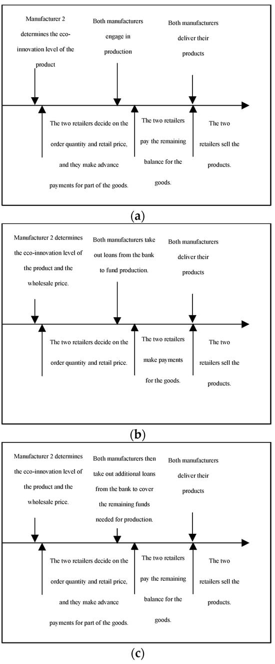
Under manufacturers’ financial constraints, to alleviate their own financial pressures, capital-constrained manufacturers can be financed through three methods as depicted in Figure 1: internal financing (advance payments from downstream retailers), bank financing, and mixed financing.
Figure 1.
Sequence of events under the three financing modes. (a) Internal financing mode, (b) Internal financing mode, (c) Internal financing mode.
- Related parameters:
To differentiate parameters across various modes, this study uses subscripts as follows: denotes Manufacturer 1’s power structure, denotes Manufacturer 2’s power structure, denotes the internal financing mode, denotes the bank financing mode, and denotes the mixed financing mode. Product 1 refers to conventional products, while Product 2 refers to eco-innovative products.
: Unit retail prices of Product 1 and Product 2.
: Market demand quantities for Product 1 and Product 2, .
,: Unit wholesale prices of Product 1 and Product 2.
: Profits of Manufacturer 1 and Manufacturer 2.
: Profits of Retailer 1 and Retailer 2.
: Total profit of the supply chain, defined as the sum of profits of the two manufacturers and two retailers.
: Innovation level of Product 2.
: One-time upfront innovation investment cost coefficient for Manufacturer 2.
: Coefficient of unit production cost for Manufacturer 2.
: Initial capital level of manufacturers.
: Coefficient of consumer environmental awareness.
: Sensitivity of consumers to the additional utility of Product 2, following a uniform distribution on [0, 1].
: Discount rate for advance payments made by retailers.
: Proportion of advance payments made by retailers.
: Bank loan interest rate.
Supply Chain Decisions under Two Different Power Structures
2.3. Supply Chain Decisions Dominated by Manufacturer 1
Under Manufacturer 1’s dominant power structure, Manufacturer 2 first determines the eco-innovation level of Product 2. Subsequently, under the condition that the price of Product 1 is fixed, Manufacturer 2 enters the market to compete with Manufacturer 1. Therefore, the game is divided into three stages: in the first stage, Manufacturer 2 determines the eco-innovation level of the product; in the second stage, after Manufacturer 1 determines the wholesale price, Manufacturer 2 decides the wholesale price of Product 2 based on the wholesale price of Product 1; in the third stage, after Retailer 1 determines the retail price, Retailer 2 determines the retail price of Product 2 based on the retail price of Product 1 (As shown in Figure 2).
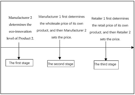
Figure 2.
A three-stage game diagram under the dominant power structure of Manufacturer 1.
This study employs a backward induction method for solution.
2.3.1. Internal Financing Mode
In the internal financing mode (as shown in Figure 1a), retailers support manufacturers’ financing needs by paying a portion of the goods’ cost upfront. The retailer’s advance payment ratio and the discount ratio obtained by the retailer for early payment are exogenous variables, typically influenced by industry norms and bargaining power between parties. After receiving the retailers’ advance payment, manufacturers proceed with product innovation and production. The discount benefit received by the retailer due to early payment is. ( variables definitions can be found in the Appendix A).
- (1)
- Internal Financing Mode with Sufficient Capital
Manufacturer 1 satisfies . Manufacturer 2’s initial capital level is .
The profit functions for Retailer 1 and Manufacturer 1 of Product 1 are as follows:
The profit functions for Retailer 2 and Manufacturer 2 of Product 2 are as follows:
Using the backward induction method to solve, we obtain the following:
Proposition 1.
When Manufacturer 2’s initial capital is in the range [, , the equilibrium decisions of Manufacturer 2 and Retailer 2 for Product 2 are as follows (Please refer to the Appendix A for the proof of Proposition 1):
Thus, when Manufacturer 2’s initial capital falls within the range [,, the following inequality holds: .
When the initial capital of Manufacturer 1 falls within the range [,, the equilibrium decisions for Manufacturer 1 and Retailer 1 regarding Product 1 are as follows:
where
Thus, when Manufacturer 1’s initial capital falls within the range [,, the following inequality holds: .
Corollary 1.
Under the internal financing model led by Manufacturer 1, the profits for Manufacturer 1 and Retailer 1 of Product 1, as well as the profits for Manufacturer 2 and Retailer 2 of Product 2, are as follows:
- (2)
- Internal Financing Mode with Insufficient Capital
When the initial capital levels of the two manufacturers satisfy , we obtain the following (Please refer to the Appendix A for the proof of Proposition 2):
Proposition 2.
Under the internal financing model, when the initial capital of Manufacturer 2 is below the threshold, the equilibrium decisions for Manufacturer 2 and Retailer 2 regarding Product 2 are as follows:
The equilibrium decisions for Manufacturer 1 and Retailer 1 of Product 1 are as follows:
where
Conclusion 1: In Propositions 1 and 2, manufacturers’ order quantities are identical and independent of the coefficient related to one-time innovation investment costs. Manufacturer 2 can flexibly adjust the level of product innovation and product prices to ensure market share. The variation in does not affect market preference choices.
Conclusion 2: By comparing the equilibrium decisions of manufacturers and retailers in Proposition 1 and Proposition 2, we conclude that when the initial capital level of Manufacturer 2 is above a certain threshold, the initial capital of the manufacturer does not affect the balanced decisions of the supply chain under financial constraints. Instead, the discount rate for retailers’ advance payments and the advance payment ratio only affect the wholesale price of the product. However, when the initial capital level of Manufacturer 2 is below this threshold, both the initial capital of the manufacturer and the discount rate for retailers’ advance payments and the advance payment ratio affect the balanced decisions of the supply chain under financial constraints. The underlying logic is that when the initial capital level of Manufacturer 2 is above a certain threshold, Manufacturer 2 does not require additional financial support from retailers and has stronger negotiation power to increase the wholesale price of innovative products, thereby recapturing the discount benefits obtained by retailers. On the other hand, when the initial capital level of Manufacturer 2 is below this threshold, Manufacturer 2 requires more financial support from retailers, weakening its negotiation power. In this scenario, the manufacturer cannot increase the wholesale price of innovative products to recoup the discount benefits obtained by retailers.
2.3.2. Bank Financing Model
Manufacturers can opt to be financed through banks, introducing external funds. Under the bank financing model (as shown in Figure 1b), manufacturers borrow from banks to invest in innovation and product manufacturing. They repay the bank loans plus interest after sales are completed. The bank loan interest rate is treated as an exogenous variable in this study. It is assumed that under the bank financing model, banks, as providers of external funds, can supply sufficient capital through loan services.
The profit functions for Retailer 1 and Manufacturer 1 of Product 1 are as follows:
The profit functions for Retailer 2 and Manufacturer 1 of Product 2 are as follows:
Similarly, we can obtain the following:
Proposition 3.
Under the bank financing model led by Manufacturer 1, the equilibrium decisions for Manufacturer 2 and Retailer 2 regarding Product 2 are as follows:
The equilibrium decisions for Manufacturer 1 and Retailer 1 of Product 1 are as follows:
Corollary 2.
>Under the bank financing model led by Manufacturer 1, the profits for Manufacturer 1 and Retailer 1 of Product 1, as well as the profits for Manufacturer 2 and Retailer 2 of Product 2, are as follows:
2.3.3. Hybrid Financing Model
Under the hybrid financing model (as shown in Figure 1c), the financially constrained manufacturer first raises funds through internal financing amounting to and then borrows the remaining funds from the bank. After sales are completed, the manufacturer repays the bank loan along with the interest.
The profit functions for Retailer 1 and Manufacturer 1 of Product 1 are as follows:
The profit functions for Retailer 2 and Manufacturer 2 of Product 1 are as follows:
Using the backward induction method to solve, we similarly obtain the following:
Proposition 4.
Under the hybrid financing model dominated by Manufacturer 1, the equilibrium decisions for Manufacturer 2 and Retailer 2 regarding Product 2 are as follows:
The equilibrium decisions for Manufacturer 1 and Retailer 1 of Product 1 are as follows:
2.4. Supply Chain Decisions Dominated by Manufacturer 2
Under the power structure dominated by Manufacturer 2, Manufacturer 2 first decides on the level of eco-innovation for Product 2 and the wholesale price of Product 2. Manufacturer 1 then determines the wholesale price of Product 1 based on the eco-innovation level and wholesale price of Product 2. Therefore, the game is divided into three stages: in the first stage, Manufacturer 2 decides on the eco-innovation level of the product; in the second stage, after Manufacturer 2 determines the wholesale price, Manufacturer 1 decides on the wholesale price of Product 1 based on the wholesale price of the innovative product; in the third stage, after Retailer 2 sets the retail price, Retailer 1 determines the retail price of Product 1 based on the retail price of Product 2(As shown in Figure 3). This study uses the backward induction method to solve the problem.
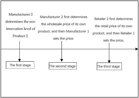
Figure 3.
A three-stage game diagram under the dominant power structure of Manufacturer 2.
2.4.1. Internal Financing Model
Under the internal financing model (as shown in Figure 1a), retailers support the manufacturers’ financing needs by paying part of the payment in advance. The advance payment ratio and the discount ratiothat retailers receive for advance payment are exogenous variables, influenced by the industry’s inherent rules and the bargaining power of both parties. After receiving the advance payment from the retailers, manufacturers conduct product innovation and production. The discount benefit obtained by retailers for advance payment is .
- (1)
- Internal Financing Mode with Sufficient Capital
Assume that under the internal financing model, Manufacturer 1 satisfies . The initial capital level of Manufacturer 2 is .
The profit functions for Retailer 1 and Manufacturer 1 of Product 1 are as follows:
The profit functions for Retailer 2 and Manufacturer 2 of Product 2 are as follows:
Using backward induction to solve, we obtain the following:
Proposition 5.
When the initial capital of Manufacturer 2 is within the range [, , the equilibrium decisions for Manufacturer 2 and Retailer 2 of Product 2 are as follows (Please refer to the Appendix A for the proof of Proposition 5):
To ensure that the initial capital of Manufacturer 2 is within the range [,, it holds that .
When the initial capital of Manufacturer 1 is within [,, the equilibrium decisions for Manufacturer 1 and Retailer 1 of Product 1 are as follows:
where
Thus, ensuring that when the initial capital of Manufacturer 1 is within [,, it holds that .
Corollary 3.
Under Manufacturer 2’s leadership in the internal financing model, the profits of Manufacturer 1 and Retailer 1 of Product 1, as well as Manufacturer 2 and Retailer 2 of Product 2, are as follows:
- (2)
- Internal Financing Mode with Insufficient Capital
When the initial capital levels of both manufacturers are within , we obtain the following:
Proposition 6.
Under the internal financing model, when the initial capital of Manufacturer 2 is below the threshold , the equilibrium decisions for Manufacturer 2 and Retailer 2 of Product 2 are as follows (Please refer to the Appendix A for the proof of Proposition 6):
Therefore, when the initial capital of Manufacturer 1 is within [, , the equilibrium decisions for Manufacturer 1 and Retailer 1 of Product 1 are as follows:
2.4.2. Bank Financing Model
In the bank financing model (as shown in Figure 1b), manufacturers borrow funds from the bank to invest in innovation and produce products. After the sales are completed, they repay the bank loan along with interest, where the bank loan interest rate is an exogenous variable. This study assumes that under the bank financing model, the bank, as the external capital provider, can supply sufficient funds.
The profit functions for Retailer 1 and Manufacturer 1 of Product 1 are as follows:
The profit functions for Retailer 2 and Manufacturer 2 of Product 2 are as follows:
Similarly, we can obtain the following:
Proposition 7.
Under the bank financing model, the equilibrium decisions for Manufacturer 2 and Retailer 2 of Product 2 are as follows:
The equilibrium decisions for Manufacturer 1 and Retailer 1 of Product 1 are as follows:
Corollary 4.
Under the bank financing model dominated by Manufacturer 2, the profits for Manufacturer 1 and Retailer 1 of Product 1, and Manufacturer 2 and Retailer 2 of Product 2, are as follows:
2.4.3. Hybrid Financing Model
In the hybrid financing model (as shown in Figure 1c), the capital-constrained manufacturer first raises funds through internal financing, obtaining an amount of . Subsequently, the manufacturer borrows the remaining funds from the bank. After the sales are completed, the manufacturer repays the bank loan along with interest.
The profit functions for Retailer 1 and Manufacturer 1 of Product 1 are as follows:
The profit functions for Retailer 2 and Manufacturer 2 of Product 1 are as follows:
By solving using the method of backward induction, we can derive the following results:
Proposition 8.
Under the hybrid financing model, the equilibrium decisions for Manufacturer 2 and Retailer 2 of Product 2 are as follows:
Under the hybrid financing model, the equilibrium decisions for Manufacturer 1 and Retailer 1 of Product 1 are as follows:
3. Comparative Study of Different Power Structures and Financing Models
Based on Table 1, Conclusion 3 can be drawn.

Table 1.
Comparison of supply chain optimization operation decisions under different power structures and financing modes.
- Conclusion 3:
- When , compared to Manufacturer 1’s dominant power structure, Manufacturer 2’s dominant power structure leads to a higher market share for Product 1 and a lower market share and innovation level for Product 2.
- Compared to Manufacturer 1’s dominant power structure, Manufacturer 2’s dominant power structure results in lower wholesale and retail prices for any product.
- When, compared to the internal financing mode, the banking financing mode leads to a higher market share for Product 1 and a lower market share and innovation level for Product 2.
- Regardless of the financing mode and power structure, an increase in positively impacts the prices and innovation level of any product.
- Manufacturer 1 does not invest in product innovation, but the price of Product 1 increases with an increase in , indicating that Manufacturer 1 engages in “free-riding” behavior.
4. Numerical Simulation
Considering the complexity of the equations listed, MATLAB software was employed as a computational tool to solve each formula. Numerical analysis was conducted to examine the impact of the manufacturer’s one-time innovation cost coefficient , unit production cost coefficient , and the market acceptance of Product 2. The objective was to derive favorable conclusions to provide decision-making insights for government entities and stakeholders within the supply chain.
4.1. Impact of k, t, and m on the Thresholds B1ex and B2ex in the Internal Financing Mode
Assuming , , , , , , .
Figure 4a illustrates that under any power structure and financing mode, as consumer environmental awareness coefficient k increases, Manufacturer 2’s threshold for internal funds shows a rising trend, while Manufacturer 1’s threshold shows a declining trend. The underlying rationale is that with sufficient funds, manufacturers can choose to adjust their product’s eco-innovation level or product prices to maintain market share. As consumer environmental awareness increases, product prices rise. Therefore, Manufacturer 2 opts to increase its product’s eco-innovation level with increasing k to maintain market share, resulting in higher overall production costs for Manufacturer 2 and, thus, an increase in their internal fund threshold. Concurrently, as Manufacturer 2’s product eco-innovation level rises, Manufacturer 1 exhibits a “free-rider” behavior where the wholesale price of Product 1 increases with the wholesale price of Product 2, leading to increased advance payments from retailers to Manufacturer 1 and, consequently, a decrease in their internal fund threshold.
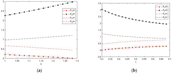
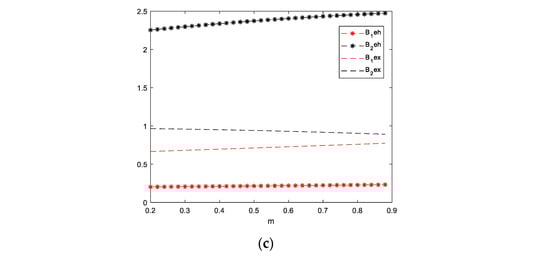
Figure 4.
Impact of , , and on the threshold of self-owned funds. (a) Impact of on the threshold of self–owned funds, (b) Impact of on the threshold of self–owned funds, (c) Impact of on the threshold of self–owned funds.
Figure 4b indicates that under any power structure and financing mode, as Manufacturer 2’s one-time innovation investment cost coefficient t increases, Manufacturer 2’s internal fund threshold shows a decreasing trend, while Manufacturer 1’s internal fund threshold shows an increasing trend. The underlying logic is that when the consumer environmental awareness coefficient remains constant, Manufacturer 2’s product eco-innovation level decreases with increasing t, reducing Manufacturer 2’s overall production costs and, thus, decreasing their internal fund threshold. A decrease in innovation level for the innovative product will lower the wholesale price of Product 1, thereby increasing Manufacturer 1’s internal fund threshold.
Figure 4c demonstrates that under Manufacturer 1’s dominant power structure, as the unit production cost coefficient of Manufacturer 2 increases, Manufacturer 2’s threshold for its own funds shows a continuous upward trend, while Manufacturer 1’s threshold also shows a slight upward trend. In Manufacturer 2’s dominant power structure, with an increase in, Manufacturer 2’s threshold for its own funds exhibits a continuous downward trend, whereas Manufacturer 1’s threshold shows a continuous upward trend. The primary reason for the differing trends in Manufacturer 2’s own fund thresholds under different power structures lies in the decrease in innovation level of Product 2 as increases. This decrease in Product 2’s innovation level not only reduces Manufacturer 2’s innovation investment costs but also decreases the amount of advance payments from Retailer 2 to Manufacturer 2. Consequently, when the reduction in advance payments for Product 2 exceeds the reduction in Manufacturer 2’s innovation investment costs, Manufacturer 2’s own fund threshold shows a continuous upward trend; otherwise, it shows a continuous downward trend.
Figure 4 illustrates that irrespective of parameter variations, Manufacturer 1’s dominant power structure imposes the highest requirement on Manufacturer 2’s own fund threshold and the lowest requirement on Manufacturer 1’s own fund threshold. In contrast, Manufacturer 2’s dominant power structure positions the requirement for Manufacturer 2’s own fund threshold between these two scenarios. Moreover, with an increase in parameters and , the requirement for Manufacturer 2’s own fund threshold transitions from being higher than Manufacturer 1’s own fund threshold requirement to being lower. This transition is due to Product 1’s higher market share compared to Product 2 under Manufacturer 2’s dominant power structure, resulting in increased total costs for producing Product 1.
4.2. The Impact of k, t, and m on the Financing Decisions of Capital-Constrained Manufacturers
From Section 4.1, under internal financing, this study restrictsin , in , and in to ensure the premise exists for analysis. Then, Section 4.1 divides into three intervals: [,, [,, and [,. This study examines the financing decisions of capital-constrained manufacturers under three scenarios: , and . It was found that these scenarios do not fundamentally alter the final choice of power structure and financing decision. When , the internal financing mode with insufficient capital does not meet the constraint conditions for Manufacturer 1’s dominant power structure with the given parameters, and the overall supply chain profit is the lowest for Manufacturer 2’s dominant power structure under the internal financing mode with insufficient capital. When , the internal financing mode with insufficient capital does not meet the constraint conditions for both power structures with the given parameters. This indicates that if manufacturers have low own funds and the market only has an internal financing model, eco-innovation in the market will be difficult to occur. Therefore, this study only shows the numerical simulation results when the capital-constrained manufacturer has own funds in [,, setting , , , , , , , and .
Figure 5a shows that under any power structure and financing model, as the consumer environmental awareness coefficient increases, the eco-innovation level of product 2 rises continuously. In a Manufacturer 1-dominated power structure, the mixed financing model achieves the highest eco-innovation level for Product 2. In contrast, under the internal financing mode with insufficient capital, Product 2’s eco-innovation level is initially higher than in any financing model dominated by Manufacturer 2, but it is eventually surpassed by the Manufacturer 2-dominated models. In a Manufacturer 2-dominated power structure, the internal financing mode with sufficient capital achieves the highest eco-innovation level for Product 2.
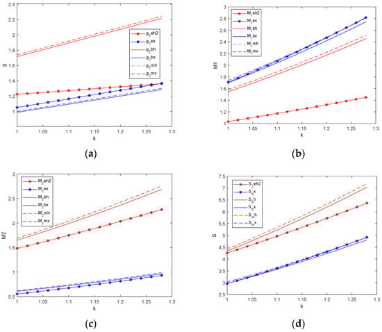
Figure 5.
Impact of on the financing decision of capital-constrained manufacturers. (a) Impact of on Product 2’s eco-innovation level, (b) Impact of on Manufacturer 1’s profit, (c) Impact of on Manufacturer 2’s profit, (d) Impact of on overall supply chain profit.
Figure 5b indicates that under any power structure and financing model, as increases, Manufacturer 1’s profit rises continuously. In a Manufacturer 1-dominated power structure, the mixed financing model yields the highest profit for Manufacturer 1. In a Manufacturer 2-dominated power structure, the profits for Manufacturer 1 across the three financing models do not differ significantly, but the profit growth rate is higher under the internal financing mode with sufficient capital. Overall, compared to a Manufacturer 1-dominated power structure, Manufacturer 1’s profit is generally higher under a Manufacturer 2-dominated power structure. This is because, under a Manufacturer 1-dominated power structure, Product 1’s market share is lower.
Figure 5c shows that under any power structure and financing model, as increases, Manufacturer 2’s profit also rises continuously. In a Manufacturer 1-dominated power structure, the mixed financing model yields the highest profit for Manufacturer 2. In a Manufacturer 2-dominated power structure, Manufacturer 2’s profits across the three financing models do not differ significantly, but the mixed financing model yields the highest profits, whereas the profit growth rate under the internal financing mode with sufficient capital is faster. Overall, compared to a Manufacturer 1-dominated power structure, Manufacturer 2’s profit is generally lower under a Manufacturer 2-dominated power structure.
Figure 5d shows that under any power structure and financing model, as increases, the overall profit of the supply chain rises continuously. In a Manufacturer 1-dominated power structure, the mixed financing model achieves the highest overall supply chain profit. In a Manufacturer 2-dominated power structure, the overall supply chain profits do not differ significantly across the three financing models. However, the overall profit growth rate under the internal financing mode with sufficient capital is the fastest, eventually surpassing the other financing models. Overall, compared to a Manufacturer 1-dominated power structure, the overall supply chain profit is generally lower under a Manufacturer 2-dominated power structure.
Figure 5 indicates that under any power structure and financing model, as increases, the eco-innovation level of Product 2, Manufacturer 1’s profit, Manufacturer 2’s profit, and the overall supply chain profit all rise continuously. This implies that an increase in the consumer environmental awareness coefficient is beneficial for all participants in the supply chain. Additionally, under a Manufacturer 2-dominated power structure, the internal financing model has the lowest capital cost, the highest eco-innovation level for Product 2, but the lowest profit for Manufacturer 2. The underlying reason is that when , there is excess capital underutilized by Manufacturer 2 in a Manufacturer 2-dominated power structure. This also explains why, compared to other financing models, the internal financing model under Manufacturer 2 sees the fastest profit growth rate as increases, as Manufacturer 2 utilizes excess capital to generate profit. Finally, in terms of power structure choice, a Manufacturer 1-dominated structure is optimal for the overall supply chain but not for Manufacturer 1. In terms of financing model choice, the mixed financing model is optimal for the overall supply chain.
Figure 6a shows that under any power structure and financing model, as Manufacturer 2’s one-time innovation investment cost coefficient increases, the eco-innovation level of Product 2 decreases continuously. In a Manufacturer 1-dominated power structure, the mixed financing model achieves the highest eco-innovation level for Product 2, but the internal financing mode with insufficient capital has the slowest decline in the eco-innovation level. In a Manufacturer 2-dominated power structure, the internal financing mode with sufficient capital achieves the highest eco-innovation level for Product 2.
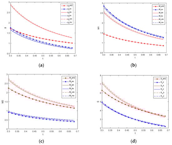
Figure 6.
Impact of on the financing decision of capital-constrained manufacturers. (a) Impact of on Product 2’s eco-innovation level, (b) Impact of on Manufacturer 1’s profit, (c) Impact of on Manufacturer 2’s profit, (d) Impact of on overall supply chain profit.
Figure 6b indicates that under any power structure and financing model, as increases, Manufacturer 1’s profit declines continuously. In a Manufacturer 1-dominated power structure, the mixed financing model yields the highest profit for Manufacturer 1. In a Manufacturer 2-dominated power structure, the profits for Manufacturer 1 across the three financing models do not differ significantly, but the profit decline rate is higher under the internal financing mode with sufficient capital. Overall, compared to a Manufacturer 1-dominated power structure, Manufacturer 1’s profit is generally higher under a Manufacturer 2-dominated power structure.
Figure 6c shows that under any power structure and financing model, as increases, Manufacturer 2’s profit also declines continuously. In a Manufacturer 1-dominated power structure, the mixed financing model yields the highest profit for Manufacturer 2, but the internal financing mode with insufficient capital has the slowest decline in Manufacturer 2’s profit. In a Manufacturer 2-dominated power structure, Manufacturer 2’s profits across the three financing models do not differ significantly, but the mixed financing model yields the highest profits, whereas the profit decline rate under the internal financing mode with sufficient capital is faster. Overall, compared to a Manufacturer 1-dominated power structure, Manufacturer 2’s profit is generally lower under a Manufacturer 2-dominated power structure.
Figure 6d shows that under any power structure and financing model, as increases, the overall profit of the supply chain declines continuously. In a Manufacturer 1-dominated power structure, the internal financing mode with insufficient capital has the slowest decline in overall supply chain profit, so as increases, the overall profit of the supply chain in the internal financing mode with insufficient capital initially falls below but eventually surpasses other financing models. This indicates that for the overall supply chain, as the one-time innovation investment cost rises, the total external financing cost becomes too high, making direct production with existing funds the optimal decision. In a Manufacturer 2-dominated power structure, the overall supply chain profits do not differ significantly across the three financing models. Overall, compared to a Manufacturer 1-dominated power structure, the overall supply chain profit is generally lower under a Manufacturer 2-dominated power structure.
Figure 6 indicates that under any power structure and financing model, as increases, the eco-innovation level of Product 2, Manufacturer 1’s profit, Manufacturer 2’s profit, and the overall supply chain profit all decline continuously. This implies that an increase in Manufacturer 2’s one-time innovation investment cost is detrimental to all participants in the supply chain. In terms of power structure choice, a Manufacturer 1-dominated structure is optimal for the overall supply chain but not for Manufacturer 1. In terms of financing model choice, when, the mixed financing model is optimal for the overall supply chain. When , the internal financing mode with insufficient capital is optimal for the overall supply chain.
Figure 7a shows that under any power structure and financing model, as Manufacturer 2’s unit production cost coefficient increases, the eco-innovation level of Product 2 continuously decreases. In a Manufacturer 1-dominated power structure, the mixed financing model achieves the highest eco-innovation level for Product 2, but the internal financing mode with insufficient capital has the fastest decline in the eco-innovation level. In a Manufacturer 2-dominated power structure, the internal financing mode with sufficient capital achieves the highest eco-innovation level for Product 2.
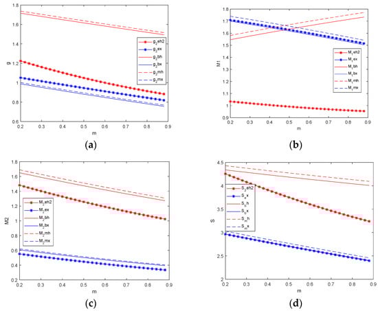
Figure 7.
Impact of on the financing decision of capital-constrained manufacturers. (a) Impact of on Product 2’s eco-innovation level, (b) Impact of on Manufacturer 1’s profit, (c) Impact of on Manufacturer 2’s profit, (d) Impact of on overall supply chain profit.
Figure 7b indicates that in a Manufacturer 1-dominated power structure, as increases, Manufacturer 1’s profit in the mixed financing and bank financing models continuously rises, whereas in the internal financing mode with insufficient capital, Manufacturer 1’s profit continuously declines. In a Manufacturer 2-dominated power structure, as increases, Manufacturer 1’s profit continuously declines across all financing models. The differing profit trends under different power structures are due to the changes in wholesale price formulas, which subsequently affect Manufacturer 1’s profit trends. The decline in Manufacturer 1’s profit in the internal financing mode with insufficient capital is because Manufacturer 1’s lack of funds reduces its bargaining power, increasing internal financing costs, and transferring funds to Retailer 1. Overall, as increases, Manufacturer 1’s profit in a Manufacturer 1-dominated power structure shifts from initially lower to ultimately higher than in a Manufacturer 2-dominated power structure. In both power structures, the mixed financing model yields the highest profit for Manufacturer 1.
Figure 7c shows that under any power structure and financing model, as increases, Manufacturer 2’s profit continuously declines. In a Manufacturer 1-dominated power structure, the mixed financing model yields the highest profit for Manufacturer 2, but the internal financing mode with insufficient capital has the fastest decline in Manufacturer 2’s profit. In a Manufacturer 2-dominated power structure, Manufacturer 2’s profits across the three financing models do not differ significantly, but the mixed financing model yields the highest profit. Overall, compared to a Manufacturer 1-dominated power structure, Manufacturer 2’s profit is generally lower in a Manufacturer 2-dominated power structure.
Figure 7d shows that under any power structure and financing model, as increases, the overall profit of the supply chain continuously declines. In a Manufacturer 1-dominated power structure, the mixed financing model achieves the highest overall supply chain profit, while the internal financing mode with insufficient capital has the fastest decline in overall supply chain profit. In a Manufacturer 2-dominated power structure, the overall supply chain profits across the three financing models do not differ significantly, with the mixed financing model achieving the highest overall supply chain profit. Overall, compared to a Manufacturer 1-dominated power structure, the overall supply chain profit is generally lower in a Manufacturer 2-dominated power structure.
Figure 7 illustrates that except for the mixed and bank financing models in a Manufacturer 1-dominated power structure, the eco-innovation level of Product 2, Manufacturer 1’s profit, Manufacturer 2’s profit, and the overall supply chain profit continuously decline with increasing . As increases, in terms of power structure choice, a Manufacturer 1-dominated power structure is optimal for the overall supply chain but only beneficial for Manufacturer 1 when , which would reduce the profits of other participants, especially as Manufacturer 2’s profit will gradually fall below Manufacturer 1’s profit. In terms of financing model choice, the mixed financing model is optimal for the overall supply chain.
Figure 5, Figure 6 and Figure 7 indicate that when Manufacturer 2 has self-owned funds , both manufacturers find mixed financing most beneficial for funding. However, the two manufacturers have differing preferences for power structure; Manufacturer 1 prefers a Manufacturer 2-dominated structure, while Manufacturer 2 prefers a Manufacturer 1-dominated structure, with the overall supply chain favoring a Manufacturer 1-dominated structure. Additionally, an increase in consumer environmental awareness benefits all participants in the supply chain, while an increase in Manufacturer 2’s one-time innovation investment cost is detrimental to all participants. An increase in Manufacturer 2’s unit production cost is advantageous for Manufacturer 1 in a Manufacturer 1-dominated structure but disadvantageous for all participants in a Manufacturer 2-dominated structure. These insights can guide the Chinese government in adjusting power structures in the eco-innovation industry.
5. Conclusions
In this study, we employ a Stackelberg game model to investigate the optimal financing decisions for capital-constrained manufacturers under different power structures, focusing particularly on the operational strategies of eco-innovative firms and conventional firms at various levels of self-owned capital. The key conclusions of the study are as follows:
- Compared to the power structure dominated by conventional firms, the power structure dominated by eco-innovative firms significantly enhances the level of eco-innovation in products and the overall profitability of the supply chain.
- When eco-innovative firms have ample funds, the cost of internal financing is the lowest, but it can lead to idle funds. Bank financing and mixed financing modes have higher financing costs but better capital utilization.
- When eco-innovative firms are undercapitalized, the mixed financing mode becomes the optimal choice due to its excellent balance between financing costs and capital efficiency.
This research constructs Stackelberg game models for six scenarios involving three financing modes under different power structures, filling the gap in existing studies by integrating consumer behavior, corporate financing constraints, and power structures. It enriches the research content in the intersection of innovation management and supply chain finance. Additionally, this study provides a detailed numerical simulation analysis, revealing the impacts of various factors on the equilibrium state regarding the level of product eco-innovation, manufacturer profits, and overall supply chain profits under different levels of self-owned capital. These findings offer valuable references for policymakers and corporate managers.
However, the study has certain limitations:
- The assumptions and parameter settings used in the model may not fully capture all the complexities and variations present in actual supply chains.
- Our analysis primarily focuses on the impacts of financing constraints and power structures on eco-innovative firms, without adequately considering market demand fluctuations, policy changes, and other external environmental factors.
- The parameters such as the consumer environmental awareness coefficient , the one-time innovation investment cost coefficient , and the unit production cost coefficient are somewhat idealized, and more variables and uncertainties may exist in practical applications.
Future research can further expand the model to encompass more real-world uncertainties, such as market demand fluctuations and policy changes. Additionally, exploring the impact of policies from different countries and regions on the financing decisions of eco-innovative firms could provide more targeted recommendations for enterprises in various contexts. Moreover, analyzing the optimal decisions of other types of firms (e.g., small and medium-sized enterprises and startups) under different financing modes could broaden the application scenarios of the research.
In summary, this study, through theoretical modeling and numerical simulations, delves into the optimal financing decisions for capital-constrained manufacturers under different power structures, providing valuable guidance for the financing decisions of eco-innovative firms and policy formulation. Nonetheless, future research needs to integrate more real-world data and contexts to further refine and expand the research model, thereby enhancing its practicality and applicability.
Author Contributions
Writing—original draft preparation, H.H.; writing—review and editing, Z.D.; supervision, N.X. All authors have read and agreed to the published version of the manuscript.
Funding
This research was funded by [The National Natural Science Foundation of China, Youth Project] grant number [71901094]; [The General Project of the Hunan Provincial Natural Science] grant number [CX2023047] and [The Youth Project of the Hunan Provincial Natural Science Foundation] grant number [2020JJ5378].
Data Availability Statement
Data is unavailable due to privacy or ethical restrictions.
Conflicts of Interest
The authors declare no conflict of interest.
Appendix A
Proof of Proposition 1.
First, starting from the third stage of the game, based on the basic assumptions, it is easy to derive , . Substituting into , and taking the first derivative with respect to and setting it to zero, we obtain
Substituting and into , and taking the first derivative with respect to and setting it to zero, we obtain
Substituting , , and into , and taking the first derivative with respect to and setting it to zero, we obtain
Substituting , , , and into , and taking the first derivative with respect to and setting it to zero, we obtain
This study substitutes , , , , and into and obtains the first-order derivative with respect to , which when set to zero yields
□
Proof of Proposition 2.
By substituting and into the constraint we obtain
Let ,
Since .
Let such that , i.e., Solving this quadratic equation, we obtain
where . □
Proof of Proposition 5.
Start from the third stage of the game. According to the basic assumptions, we obtain , . Substituting into and setting the first derivative of to zero, we obtain
Next, substituting , and into , and setting the first derivative with respect to to zero, we obtain
Subsequently, substituting , and into , and setting the first derivative with respect to to zero, we obtain
Further, substituting , , , and into , and setting the first derivative with respect to to zero, we obtain
Finally, substituting , , , , and into , and setting the first derivative with respect to to zero, we obtain
□
Proof of Proposition 6.
Substituting , into the constraint , we obtain
Let ,
where , .
Since .
Set to ensure .
Solving this quadratic equation gives
where .
Variable definitions
□
References
- Freeman, C. The Economics of Industrial Innovation, 2nd ed.; Frances Printer: London, UK, 1982. [Google Scholar]
- Reutterer, T.; Platzer, M.; Schröder, N. Leveraging purchase regularity for predicting customer behavior the easy way. Int. J. Res. Mark. 2021, 38, 194–215. [Google Scholar] [CrossRef]
- Featherman, M.; Jia, S.J.; Califf, C.B.; Hajli, N. The impact of new technologies on consumers beliefs: Reducing the perceived risks of electric vehicle adoption. Technol. Forecast. Soc. Chang. 2021, 169, 120847. [Google Scholar] [CrossRef]
- Al-Azzam, A.F.; Al-Mizeed, K. The effect of digital marketing on purchasing decisions: A case study in Jordan. J. Asian Financ. Econ. Bus. 2021, 8, 455–463. [Google Scholar]
- Chen, Y.; Xie, J. Online consumer review: Word-of-mouth as a new element of marketing communication mix. Manag. Sci. 2008, 54, 477–491. [Google Scholar] [CrossRef]
- Cai, M.; Luo, J. Optimal Financing Strategy and Quality Decision for a Capital-Constrained Manufacturers. J. Syst. Manag. 2022, 31, 230–240. [Google Scholar]
- Chen, Z.; Liu, Z.; Suárez Serrato, J.C.; Xu, D.Y. Notching R&D investment with corporate income tax cuts in China. Am. Econ. Rev. 2021, 111, 2065–2100. [Google Scholar]
- Wang, M.; Li, Y.; Li, J.; Wang, Z. Green process innovation, green product innovation and its economic performance improvement paths: A survey and structural model. J. Environ. Manag. 2021, 297, 113282. [Google Scholar] [CrossRef]
- Che, C.; Zhang, X.; Chen, Y.; Zhao, L.; Zhang, Z. A model of waste price in a symbiotic supply chain based on Stackelberg algorithm. Sustainability 2021, 13, 1740. [Google Scholar] [CrossRef]
- Huang, F.; Hu, H.; Song, H.; Li, H.; Zhang, S.; Zhai, J. Allocation of the carbon emission abatement target in low carbon supply chain considering power structure. Sustainability 2023, 15, 10469. [Google Scholar] [CrossRef]
- Yao, F.; Yan, Y.; Teng, C. Pricing Decision for Closed-loop Supply Chain Considering Corporate Social Responsibility and Channel Power Structure. Manag. Rev. 2022, 34, 283–294. (In Chinese) [Google Scholar]
- Xia, Q.; Zhi, B.; Wang, X. The role of cross-shareholding in the green supply chain: Green contribution, power structure and coordination. Int. J. Prod. Econ. 2021, 234, 108037. [Google Scholar] [CrossRef]
- Liu, J.; Fu, K.; Xu, J. Impacts of power structure on the store brand entry with asymmetric information. Syst. Eng.-Theory Pract. 2021, 41, 2056–2075. (In Chinese) [Google Scholar]
- Jin, L.; Zheng, B.; Huang, S. Pricing and coordination in a reverse supply chain with online and offline recycling channels: A power perspective. J. Clean. Prod. 2021, 298, 126786. [Google Scholar] [CrossRef]
- Chen, K.; Kong, Y.; Lei, D. Pricing and green input decisions of a competitive supply chain with consumers’ product preference and different channel powers. Chin. J. Manag. Sci. 2022, 31, 1–12. [Google Scholar]
- Wang, T.; Yan, B. Decision-making of online channel from the viewpoint of game theory. J. Manag. Sci. China 2017, 6, 64–77. (In Chinese) [Google Scholar]
- Li, C.; Liu, Q.; Zhou, P.; Huang, H. Optimal innovation investment: The role of subsidy schemes and supply chain channel power structure. Comput. Ind. Eng. 2021, 157, 107291. [Google Scholar] [CrossRef]
- Wu, C.; Xu, C.; Zhao, Q.; Lin, S. Research on financing strategy of low-carbon supply chain based on cost-sharing contract. Environ. Sci. Pollut. Res. 2022, 29, 48358–48375. [Google Scholar] [CrossRef]
- Jafari, H.; Safarzadeh, S. Producing two substitutable products under a supply chain including two manufacturers and one retailer: A game-theoretic approach. J. Ind. Manag. Optim. 2023, 19, 3650–3670. [Google Scholar] [CrossRef]
- Ma, S.; Zhang, L.L.; Cai, X. Optimizing joint technology selection, production planning and pricing decisions under emission tax: A Stackelberg game model and nested genetic algorithm. Expert Syst. Appl. 2024, 238, 122085. [Google Scholar] [CrossRef]
- Das, R.; De, P.K.; Barman, A. Pricing and ordering strategies in a two-echelon supply chain under price discount policy: A Stackelberg game approach. J. Manag. Anal. 2021, 8, 646–672. [Google Scholar] [CrossRef]
- Chen, H.; Wang, J.; Miao, Y. Evolutionary game analysis on the selection of green and low carbon innovation between manufacturing enterprises. Alex. Eng. J. 2021, 60, 2139–2147. [Google Scholar] [CrossRef]
- Yang, X.; You, D. Research on enterprises green technology innovation decision—Under the perceptive of consumer environmental awareness and government subsidies. Chin. J. Manag. Sci. 2022, 30, 263–274. [Google Scholar]
- Wang, M.; Li, Y.; Cheng, Z.; Zhong, C.; Ma, W. Evolution and equilibrium of a green technological innovation system: Simulation of a tripartite game mode. J. Clean. Prod. 2021, 278, 123944. [Google Scholar] [CrossRef]
- Wei, J.; Wang, C. Improving interaction mechanism of carbon reduction technology innovation between supply chain enterprises and government by means of differential game. J. Clean. Prod. 2021, 296, 126578. [Google Scholar] [CrossRef]
- Mu, Z.; Zheng, Y.; Sun, H. Cooperative green technology innovation of an e-commerce sales channel in a two-stage supply chain. Sustainability 2021, 13, 7499. [Google Scholar] [CrossRef]
- Ju, Q.; Ju, P.; Dai, W.; Ran, L. Adoption of new energy vehicles under subsidy policies: Unit subsidies, sales incentives and product differentiation. J. Manag. Sci. China 2021, 101–116. (In Chinese) [Google Scholar] [CrossRef]
Disclaimer/Publisher’s Note: The statements, opinions and data contained in all publications are solely those of the individual author(s) and contributor(s) and not of MDPI and/or the editor(s). MDPI and/or the editor(s) disclaim responsibility for any injury to people or property resulting from any ideas, methods, instructions or products referred to in the content. |
© 2024 by the authors. Licensee MDPI, Basel, Switzerland. This article is an open access article distributed under the terms and conditions of the Creative Commons Attribution (CC BY) license (https://creativecommons.org/licenses/by/4.0/).