Dynamics of a Dengue Transmission Model with Multiple Stages and Fluctuations

Abstract

A vector–host model of dengue with multiple stages and independent fluctuations is investigated in this paper. Firstly, the existence and uniqueness of the positive solution are shown by contradiction. When the death rates of aquatic mosquitoes, adult mosquitoes, and human beings respectively control the intensities of white noises, and if ${\mathcal{R}}_0^s>1$, then the persistence in the mean for both infective mosquitoes and infective human beings is derived. When ${\mathcal{R}}_0^s>1$ is valid, the existence of stationary distribution is derived through constructing several appropriate Lyapunov functions. If the intensities of white noises are controlled and $\phi <0$ is valid, then the extinction for both infective mosquitoes and infective human beings is obtained by applying the comparison theorem and ergodic theorem. Further, the main findings are verified through numerical simulations by using the positive preserving truncated Euler–Maruyama method (PPTEM). Moreover, several numerical simulations on the infection scale of dengue in Fuzhou City were conducted using surveillance data. The main results indicate that the decrease in the transfer proportion from aquatic mosquitoes to adult mosquitoes reduces the infection scale of infective human beings with dengue virus, and the death rates of aquatic mosquitoes and adult mosquitoes affect the value of the critical threshold ${\mathcal{R}}_0^s$. Further, the controls of the death rates of mosquitoes are the effective routes by the decision-makers of the Chinese mainland against the spread of dengue.

1. Introduction

Vector-borne illnesses constitute more than 17% of all infectious diseases and cause more than 700,000 fatalities yearly, as stated in the WHO report in 2020 [1]. Dengue, commonly referred to as break-bone fever, is a vector-borne disease transmitted to human beings through mosquito bites, with Aedes aegypti and Aedes albopictus acting as the primary vectors [2]. Meanwhile, dengue acts as the most widespread mosquito-borne disease within the human population, which involves various virus serotypes from DENV-1 to DENV-4 [3]. When a mosquito carrying the dengue virus bites a human being, the severity of symptom of the human being ranges from asymptomatic to severe [2]. In fact, the yearly infection number of dengue virus is 390 million, of which 96 million infections have symptoms in the tropical and sub-tropical zones worldwide [4]. Moreover, the incidence of dengue is closely linked to climatic change and urbanization, with the prediction that an expansion of the habitat of Aedes albopictus and Aedes aegypti in the future would take place. Despite the implementation for the mitigation of climate change, the expansion of the Aedes mosquitoes may not be prevented, which implies that the world still faces the threat of dengue as claimed in [5]. As a result of climate change, up to 4.7 billion more individuals will be at risk of dengue globally in 2070 than those in the 1970s–1990s [6].

Mathematical models have increasingly become a powerful tool in the face of the great threats of infectious diseases. Dengue models and their corresponding analysis can provide a potential basis for prediction and control measures. To investigate the impacts of insecticide on dengue transmission, Newton and Reiter [7] proposed a dengue model based on the Ross–Lotka model [8]. Then, with the presence of four serotypes in dengue, Jan et al. [9] and Xue et al. [10] successively proposed the models for primary and secondary infections to study the phenomenon of limited cross-immunization among heterologous serotypes. K. Asamoah et al. [11] introduced a dengue model with partial immunization, and the optimal controls acting on the susceptible and the infected human beings were considered, the vaccination of the local population was verified effective for dengue transmission. Xue et al. [12] utilized a multi-strain model to analyze the effectiveness of human vaccination, and they accounted for the main factors such as waning immunity and vaccine failure. These dengue model studies mainly examined the virus-oriented models and the host-oriented models, while the mosquito-oriented models were equally crucial for the exploration of dengue, of which mosquitoes acted as vectors for dengue transmission. Endosymbiotic bacteria acting as the novel control method inhibited the replication of dengue within the hosts and caused the sterility in infected male mosquitoes [13]. Consequently, the models with the releasing measures of sterile mosquitoes was proposed in [14,15]. As a matter of fact, Li et al. [16] studied the fluctuations including temperature and rainfall and found that the fluctuations affected the incidence of dengue by altering the propagation of mosquitoes. Liu et al. [17] and Abdelrazec et al. [18] constructed the stage-structure mosquito models to assess the impacts of climate on mosquito dynamics. To better understand the impacts of vectors on dengue, several vector–host models incorporating multiple stages were proposed in [19,20,21,22], in which [19,21] centered around the impacts of vertical transmission on dengue outbreaks.

The epidemic models are usually established by governing ordinary differential equations (ODEs), fractional-order differential equations (FrDEs), and delay-differential equations (DDEs), as in [23,24,25,26,27], of which the deterministic models reflect the basic transmission dynamics among the distinct populations. However, the transmission dynamics is affected by the highly nonlinear and stochastic systems, in which the transmission processes of dengue is influenced by many stochastic elements such as climate variations, migration patterns, and changes in human behavior. Therefore, several stochastic models, as discussed in [28,29,30,31,32,33,34,35], have been put forward and studied in order to investigate the long-term dynamics of dengue. Otero et al. [28] discovered that the arrival date of an infected individual in the susceptible population significantly impacted the distribution of the population size of dengue, and that the probability of an early outbreak of dengue was lower. Liu et al. [31] conducted an analysis on the long-term dynamics of a dengue model by considering saturated incidence rates. Sun et al. [32] introduced the sufficient conditions for the existence of almost surely exponential stability of the disease-free equilibrium in a stochastic dengue model with independent fluctuation. Liu et al. [33] constructed a stochastic dengue model with the standard incidence rate and studied the effect of information interventions on dengue transmission. Guo et al. [34] accounted for parameter fluctuations in the dengue model and found that large fluctuations could suppress dengue transmission. It was worth noticing if weather factors like rainfall and temperature affected the growth processes of mosquitoes.

Previous contributions have not investigated dengue models with aquatic mosquitoes and independent fluctuations. We, therefore, in this paper, proposed a multi-stage vector–host model with independent fluctuations for explanations of dynamical behaviors and epidemiological implications of dengue. When fluctuations disappear, we give the expression for the basic reproduction number of the vector–host model by the next-generation matrix method in Section 2. Alternatively, we derive the long-term dynamics of the vector–host model with fluctuations, and prove the existence and uniqueness of the solution. We also derive the criteria for persistence in the mean, stationary distribution, and stochastic extinction by constructing appropriate Lyapunov functions in Section 3. Finally, we adopted 2019 surveillance data of dengue from the Fujian Provincial Center for Disease Control and Prevention (Fujian CDC). The theoretical findings were validated through numerical simulations by the PPTEM method in Section 4.

2. Model Formulation

As the vector of dengue, mosquitoes undergo four life stages, including egg, larva, pupa, and adult. Since the first three stages of mosquitoes are aquatic, we classify the egg, larva, and pupa into one group for simplicity, without losing the main characteristics [36,37]. In this study, we propose a vector–host model among the total population of human beings, the population of aquatics, and the population of adult mosquitoes for the description of the transmission mechanism of dengue. Here, the total population of mosquitoes is separated into three mutually-exclusive compartments: A, $S_m$, $I_m$, represent the number of aquatic mosquitoes, susceptible mosquitoes with no dengue infection, and infective mosquitoes, respectively. Meanwhile, three groups comprise the total human population: $S_h$, susceptible; $I_h$, infective; $R_h$, recovered. We are motivated by the aforementioned discussions on dengue models to incorporate the aquatic mosquitoes for the vector–host model:

$$\left\{\begin{array}{c}\dot{A}=\Gamma -\delta A-{\mu }_{A}A,\hfill \\ {\dot{S}}_m=\delta A-b{\beta }_m{S}_m{I}_h-{\mu }_m{S}_m,\hfill \\ {\dot{I}}_m=b{\beta }_m{S}_m{I}_h-{\mu }_m{I}_m,\hfill \\ {\dot{S}}_h=\Lambda -b{\beta }_h{S}_h{I}_m-{\mu }_h{S}_h,\hfill \\ {\dot{I}}_h=b{\beta }_h{S}_h{I}_m-\gamma I_h-{\mu }_h{I}_h,\hfill \\ {\dot{R}}_h=\gamma I_h-{\mu }_h{R}_h,\hfill \end{array}\right.$$

(1)

where $\Gamma$ and $\Lambda$ represent the constant recruitment rates of aquatic mosquitoes and human beings, respectively; ${\mu }_A$, ${\mu }_m$, and ${\mu }_h$ are the death rates of aquatic mosquitoes, adult mosquitoes, and human beings, respectively; $\delta$ expresses the maturity proportion of aquatic mosquitoes; b indicates the biting rate; ${\beta }_m$ depicts the probability of dengue virus transmitted from infective human beings to susceptible mosquitoes; ${\beta }_h$ denotes the probability of dengue virus spread from infective mosquitoes to susceptible human beings; $1/\gamma$ means the average recovery time in the human population. The definitions of the variables and the parameters in model (1) can be found in

Table 1. Descriptions of the variables to model (1).

Variable	Definition
A	Number of aquatic mosquitoes
$S_m$	Number of susceptible mosquitoes with no dengue infection
$I_m$	Number of infective mosquitoes
$S_h$	Number of susceptible human beings
$I_h$	Number of infective human beings
$R_h$	Number of recovered human beings

and

Table 2. Descriptions and source of the parameters to model (1).

Parameter	Unit	Definition	Range	Source
$\Gamma$	dimensionless	Constant recruitment rates of aquatic mosquitoes	$[0,\infty )$	/
$\Lambda$	dimensionless	Constant recruitment rates of human beings	$[0,\infty )$	/
${\mu }_A$	${\mathrm{day}}^{-1}$	Death rate of aquatic mosquitoes	$[0.01,0.47]$	[21]
$\delta$	${\mathrm{day}}^{-1}$	Maturity proportion of aquatic mosquitoes	$[0.1,0.5]$	[26]
${\mu }_m$	${\mathrm{day}}^{-1}$	Death rate of adult mosquitoes	$(0,0.3]$	[22]
$1/\gamma$	$\mathrm{day}$	Average recovery time in human population	$[4,8]$	[21]
b	${\mathrm{day}}^{-1}{\mathrm{individual}}^{-1}$	Average biting rate	$[0,1)$	/
${\beta }_m$	dimensionless	Probability of dengue virus transmitted from $I_h$ to $S_m$	$[0.3,0.75]$	[22]
${\beta }_h$	dimensionless	Probability of dengue virus spread from $I_m$ to $S_h$	$[0.1,0.75]$	[22]
${\mu }_h$	${\mathrm{day}}^{-1}$	Death rate of human beings	$[{\displaystyle \frac{1}{81\times 365}},{\displaystyle \frac{1}{50\times 365}}]$	[10,38]

.

For model (1), we derive the positive invariant set using the comparison theorems as follows:

$$\begin{array}{cc}\hfill \mathcal{D}=\left\{(A,S_m,I_m,S_h,I_h,R_h)\in {\mathbb{R}}_{+}^6:0\right.& ⩽A⩽{\displaystyle \frac{\Gamma }{\delta +{\mu }_A}},\hfill \\ \hfill 0& ⩽S_m+I_m⩽{\displaystyle \frac{\delta \Gamma }{{\mu }_m(\delta +{\mu }_A)}},\left.0⩽S_h+I_h+R_h⩽{\displaystyle \frac{\Lambda }{{\mu }_h}}\right\},\hfill \end{array}$$

and

$${\mathcal{D}}_0=\left\{(A,S_m,I_m,S_h,I_h,R_h)\in {\mathbb{R}}_{+}^6:I_m=0,I_h=0,R_h=0\right\}.$$

We investigate model (1) mainly within the invariant set $\mathcal{D}$. Let the initial values satisfy $(A\left(0\right),S_m\left(0\right),I_m\left(0\right),S_h\left(0\right),I_h\left(0\right),R_h\left(0\right))\in \mathcal{D}.$ It is easy to check that

$$P_0={(A_0,S_{m0},I_{m0},S_{h0},I_{h0},R_{h0})}^{\mathrm{T}}={\left({\displaystyle \frac{\Gamma }{\delta +{\mu }_A}},{\displaystyle \frac{\delta \Gamma }{{\mu }_m(\delta +{\mu }_A)}},0,{\displaystyle \frac{\Lambda }{{\mu }_h}},0,0\right)}^{\mathrm{T}}$$

serves as the infection-free equilibrium point. Additionally, we derive the endemic equilibrium point

$$P^{*}={(A^{*},S_m^{*},I_m^{*},S_h^{*},I_h^{*},R_h^{*})}^{\mathrm{T}}$$

under the condition $\delta b^2{\beta }_m{\beta }_h\Lambda \Gamma -{\mu }_h{\mu }_m^2(\delta +{\mu }_A)(\gamma +{\mu }_h)>0$, where

$$\begin{array}{cc}\hfill A^{*}& ={\displaystyle \frac{\Gamma }{\delta +{\mu }_A}},S_m^{*}={\displaystyle \frac{\delta \Gamma }{b{\beta }_m(\delta +{\mu }_A)I_h^{*}+{\mu }_m}},S_h^{*}={\displaystyle \frac{\Lambda }{b{\beta }_h{I}_m^{*}+{\mu }_h}},R_h^{*}={\displaystyle \frac{\gamma }{{\mu }_h}}{I}_h^{*},\hfill \\ \hfill I_m^{*}& ={\displaystyle \frac{\delta b^2{\beta }_m{\beta }_h\Lambda \Gamma -{\mu }_h{\mu }_m^2(\delta +{\mu }_A)(\gamma +{\mu }_h)}{b{\beta }_h{\mu }_m^2(\delta +{\mu }_A)(\gamma +{\mu }_h)+b^2{\beta }_m{\beta }_h{\mu }_m\Lambda (\delta +{\mu }_A)}},\hfill \\ \hfill I_h^{*}& ={\displaystyle \frac{\delta b^2{\beta }_m{\beta }_h\Lambda \Gamma -{\mu }_h{\mu }_m^2(\delta +{\mu }_A)(\gamma +{\mu }_h)}{\delta b^2{\beta }_m{\beta }_h\Gamma (\gamma +{\mu }_h)+b{\beta }_m{\mu }_h{\mu }_m(\delta +{\mu }_A)(\gamma +{\mu }_h)}}.\hfill \end{array}$$

In the set $\mathcal{D}$, we investigate the dynamical behaviors of model (1). The following is the approach by which the basic reproduction number of model (1) can be obtained from [39,40]:

$${\mathcal{R}}_0=\sqrt{{\displaystyle \frac{b^2{\beta }_m{\beta }_h\delta \Gamma \Lambda }{{\mu }_m^2{\mu }_h(\delta +{\mu }_A)(\gamma +{\mu }_h)}}}=\sqrt{{\mathcal{R}}_0^{mh}{\mathcal{R}}_0^{hm}},$$

where

$${\mathcal{R}}_0^{mh}={\displaystyle \frac{b{\beta }_h\Lambda }{{\mu }_m{\mu }_h}},{\mathcal{R}}_0^{hm}={\displaystyle \frac{b{\beta }_m\delta \Gamma }{{\mu }_m(\delta +{\mu }_A)(\gamma +{\mu }_h)}}$$

represent the average number of one infective mosquito within its lifespan effectively transmitting virus to human beings, and the average number of one infective human being before the recoverey effectively producing the infective mosquitoes, respectively.

Compared with the deterministic counterpart model (1), the fluctuations in the epidemic models offer additional insights including survival analysis [41]. In reality, the randomness of human–mosquito contacts and the randomness of human behaviors are mainly influenced from minor and independent fluctuations, such as slight variations in temperature, precipitation, wind speed, and so forth. These randomness types are usually described by the independent fluctuations when the dengue transmission is formulated. Therefore, it is necessary that the independent fluctuations are incorporated into the dengue model, which makes for more comprehensive and more accurate dengue dynamics. Moreover, stochastic dengue models assess the risks and uncertainties when different scenarios occur, and they also help the policymakers to modify control strategies. Accounting for these variations, we modify model (1) by incorporating Gaussian white noises ${\xi }_i\left(t\right)=\mathrm{d}{B}_i\left(t\right)/\mathrm{d}t$ into the dengue model, where $\mathrm{d}{B}_i\left(t\right)=B_i(t+\Delta t)-B_i\left(t\right)$ represents Brownian increments with zero mean and variance $\Delta t$. Motivated by recent studies such as [31,32,33], we let the Gaussian white noises proportional to the variables A, $S_m$, $I_m$, $S_h$, $I_h$, and $R_h$, and we take the fluctuations into account; the stochastic dengue model (2) is described with bilinear incidence rates by the following form:

$$\left\{\begin{array}{c}\mathrm{d}A\left(t\right)=[\Gamma -\delta A-{\mu }_{A}A]\mathrm{d}t+{\sigma }_{1}A\mathrm{d}{B}_1\left(t\right),\hfill \\ \mathrm{d}{S}_m\left(t\right)=[\delta A-b{\beta }_m{S}_m{I}_h-{\mu }_m{S}_m]\mathrm{d}t+{\sigma }_2{S}_m\mathrm{d}{B}_2\left(t\right),\hfill \\ \mathrm{d}{I}_m\left(t\right)=[b{\beta }_m{S}_m{I}_h-{\mu }_m{I}_m]\mathrm{d}t+{\sigma }_3{I}_m\mathrm{d}{B}_3\left(t\right),\hfill \\ \mathrm{d}{S}_h\left(t\right)=[\Lambda -b{\beta }_h{S}_h{I}_m-{\mu }_h{S}_h]\mathrm{d}t+{\sigma }_4{S}_h\mathrm{d}{B}_4\left(t\right),\hfill \\ \mathrm{d}{I}_h\left(t\right)=[b{\beta }_h{S}_h{I}_m-\gamma I_h-{\mu }_h{I}_h]\mathrm{d}t+{\sigma }_5{I}_h\mathrm{d}{B}_5\left(t\right),\hfill \\ \mathrm{d}{R}_h\left(t\right)=[\gamma I_h-{\mu }_h{R}_h]\mathrm{d}t+{\sigma }_6{R}_h\mathrm{d}{B}_6\left(t\right).\hfill \end{array}\right.$$

(2)

Here, the parameters ${\sigma }_i$ reflect the fluctuations intensities. The independent variables $B_i\left(t\right)$ are six standard Wiener processes specified on $(\Omega ,\mathcal{F},{\left\{{\mathcal{F}}_t\right\}}_{t⩾0},\mathbb{P})$. In detail, ${\left\{{\mathcal{F}}_t\right\}}_{t⩾0}$ denotes a filtration that, for any $0⩽s<t$, fulfills ${\mathcal{F}}_s\subset {\mathcal{F}}_t$, and when $B_i\left(0\right)=0$, ${\mathcal{F}}_0$ includes all $\mathbb{P}$-null sets. Moreover, we exclude the sixth equation of model (2) and focus on the equivalent stochastic epidemic following, noting that the equations of A, $S_m$, $I_m$, $S_h$, and $I_h$ in model (2) are irrespective of $R_h$. Meanwhile, we note that $U\left(t\right)=(A\left(t\right),S_m\left(t\right),I_m\left(t\right),S_h\left(t\right),I_h\left(t\right))$.

$$\left\{\begin{array}{c}\mathrm{d}A\left(t\right)=[\Gamma -\delta A-{\mu }_{A}A]\mathrm{d}t+{\sigma }_{1}A\mathrm{d}{B}_1\left(t\right),\hfill \\ \mathrm{d}{S}_m\left(t\right)=[\delta A-b{\beta }_m{S}_m{I}_h-{\mu }_m{S}_m]\mathrm{d}t+{\sigma }_2{S}_m\mathrm{d}{B}_2\left(t\right),\hfill \\ \mathrm{d}{I}_m\left(t\right)=[b{\beta }_m{S}_m{I}_h-{\mu }_m{I}_m]\mathrm{d}t+{\sigma }_3{I}_m\mathrm{d}{B}_3\left(t\right),\hfill \\ \mathrm{d}{S}_h\left(t\right)=[\Lambda -b{\beta }_h{S}_h{I}_m-{\mu }_h{S}_h]\mathrm{d}t+{\sigma }_4{S}_h\mathrm{d}{B}_4\left(t\right),\hfill \\ \mathrm{d}{I}_h\left(t\right)=[b{\beta }_h{S}_h{I}_m-\gamma I_h-{\mu }_h{I}_h]\mathrm{d}t+{\sigma }_5{I}_h\mathrm{d}{B}_5\left(t\right).\hfill \end{array}\right.$$

(3)

Next, we discuss the survival investigation of model (3) from the fitness of the global positive solution, persistence in the mean, and stationary distribution to the extinction.

3. Survival Analysis of Infective Mosquitoes and Infective Human Beings

3.1. Fitness

We primarily ensure that model (3) is well-proposed before investigating the long-term properties. That is, we show that the solution of model (3) does not blow up in Theorem 1 within the finite time by the similar method in [42,43].

Theorem 1. 

For $t⩾0$, model (3) has a unique positive solution $U\left(t\right)$ initiated with $U\left(0\right)\in {\mathbb{R}}_{+}^5$.

Proof of Theorem 1. 

According to Theorem 1 in [43], let G be a positive constant; we build up a $C^2$-function Lyapunov function $V_1$ such that $\mathcal{L}{V}_1⩽G$. Here,

$$V_1=A-1-lnA+S_m-{\theta }_1-{\theta }_{1}ln{\displaystyle \frac{S_m}{{\theta }_1}}+I_m-1-ln{I}_m+S_h-{\theta }_2-{\theta }_{2}ln{\displaystyle \frac{S_h}{{\theta }_2}}+I_h-1-ln{I}_h.$$

Since $V_1$ is non-negative, employing the generalized Itô’s formula [44], we obtain

$$\begin{array}{cc}\hfill \mathrm{d}{V}_1=& \mathcal{L}{V}_1\mathrm{d}t+(A-1){\sigma }_1\mathrm{d}{B}_1\left(t\right)+(S_m-{\theta }_1){\sigma }_2\mathrm{d}{B}_2\left(t\right)\hfill \\ & +(I_m-1){\sigma }_3\mathrm{d}{B}_3\left(t\right)+(S_h-{\theta }_2){\sigma }_4\mathrm{d}{B}_4\left(t\right)+(I_h-1){\sigma }_5\mathrm{d}{B}_5\left(t\right),\hfill \end{array}$$

where

$$\begin{array}{cc}\hfill \mathcal{L}{V}_1=& \left(1-{\displaystyle \frac{1}{A}}\right)[\Gamma -\delta A-{\mu }_{A}A]+\left(1-{\displaystyle \frac{{\theta }_1}{S_m}}\right)[\delta A-b{\beta }_m{S}_m{I}_h-{\mu }_m{S}_m]\hfill \\ \hfill & +\left(1-{\displaystyle \frac{1}{I_m}}\right)[b{\beta }_m{S}_m{I}_h-{\mu }_m{I}_m]+\left(1-{\displaystyle \frac{{\theta }_2}{S_h}}\right)[\Lambda -b{\beta }_h{S}_h{I}_m-{\mu }_h{S}_h]\hfill \\ \hfill & +\left(1-{\displaystyle \frac{1}{I_h}}\right)[b{\beta }_h{S}_h{I}_m-\gamma I_h-{\mu }_h{I}_h]+{\displaystyle \frac{1}{2}}({\sigma }_1^2+{\theta }_1{\sigma }_2^2+{\sigma }_3^2+{\theta }_2{\sigma }_4^2+{\sigma }_5^2).\hfill \end{array}$$

The appropriate simplification yields

$$\begin{array}{cc}\hfill \mathcal{L}{V}_1⩽& \Gamma +\Lambda +\delta +{\mu }_A+{\theta }_1{\mu }_m+{\mu }_m+{\mu }_h+{\theta }_2{\mu }_h+\gamma \hfill \\ \hfill & +({\theta }_{1}b{\beta }_m-{\mu }_h)I_h+({\theta }_{2}b{\beta }_h-{\mu }_m)I_m+{\displaystyle \frac{1}{2}}({\sigma }_1^2+{\theta }_1{\sigma }_2^2+{\sigma }_3^2+{\theta }_2{\sigma }_4^2+{\sigma }_5^2).\hfill \end{array}$$

We let ${\theta }_1={\displaystyle \frac{{\mu }_h}{b{\beta }_m}}$, ${\theta }_2={\displaystyle \frac{{\mu }_m}{b{\beta }_h}}$; then, we have

$$\begin{array}{cc}\hfill \mathcal{L}{V}_1⩽& \Gamma +\Lambda +\delta +{\mu }_A+{\displaystyle \frac{{\mu }_m{\mu }_h}{b{\beta }_m}}+{\mu }_m+{\mu }_h+{\displaystyle \frac{{\mu }_m{\mu }_h}{b{\beta }_h}}+\gamma \hfill \\ \hfill & +{\displaystyle \frac{1}{2}}({\sigma }_1^2+{\displaystyle \frac{{\mu }_h}{b{\beta }_m}}{\sigma }_2^2+{\sigma }_3^2+{\displaystyle \frac{{\mu }_m}{b{\beta }_h}}{\sigma }_4^2+{\sigma }_5^2):=G>0.\hfill \end{array}$$

This proof can then be easily completed by contradiction. □

3.2. Persistence in the Mean

Denote $\langle A\left(t\right)\rangle ={\displaystyle \frac{1}{t}}{\int }_0^{t}A\left(s\right)\mathrm{d}s$. Lemma 1 is obtained from the study in [41,45] without proof here.

Lemma 1. 

For $U\left(0\right)\in {\mathbb{R}}_{+}^5$, the unique solution of model (3) has the following properties:

$$\underset{t\to \infty }{lim}{\displaystyle \frac{A\left(t\right)}{t}}=0,\underset{t\to \infty }{lim}{\displaystyle \frac{S_m\left(t\right)}{t}}=0,\underset{t\to \infty }{lim}{\displaystyle \frac{I_m\left(t\right)}{t}}=0,\underset{t\to \infty }{lim}{\displaystyle \frac{S_h\left(t\right)}{t}}=0,\underset{t\to \infty }{lim}{\displaystyle \frac{I_h\left(t\right)}{t}}=0a.s..$$

If $2min\left\{{\mu }_A,{\mu }_m\right\}>max\left\{{\sigma }_1^2,{\sigma }_2^2,{\sigma }_3^2\right\}$ and $2{\mu }_h>max\left\{{\sigma }_4^2,{\sigma }_5^2\right\}$, then

$$\begin{array}{cc}\hfill & \underset{t\to \infty }{lim}{\displaystyle \frac{1}{t}}{\int }_0^{t}A\left(s\right)\mathrm{d}{B}_1\left(s\right)=0,\underset{t\to \infty }{lim}{\displaystyle \frac{1}{t}}{\int }_0^t{S}_m\left(s\right)\mathrm{d}{B}_2\left(s\right)=0,\underset{t\to \infty }{lim}{\displaystyle \frac{1}{t}}{\int }_0^t{I}_m\left(s\right)\mathrm{d}{B}_3\left(s\right)=0,\hfill \\ & \underset{t\to \infty }{lim}{\displaystyle \frac{1}{t}}{\int }_0^t{S}_h\left(s\right)\mathrm{d}{B}_4\left(s\right)=0,\underset{t\to \infty }{lim}{\displaystyle \frac{1}{t}}{\int }_0^t{I}_h\left(s\right)\mathrm{d}{B}_5\left(s\right)=0a.s..\hfill \end{array}$$

(4)

Persistence is an important behavior in many systems, which indicates how long the system remains in a certain state before it transits to another state. By using the approach in [35,46], we subsequently provide the sufficient conditions of persistence in the mean for infective mosquitoes and infective human beings of model (3). Let

$${\mathcal{R}}_0^s={\mathcal{R}}_0^{smh}{\mathcal{R}}_0^{shm},$$

where

$${\displaystyle {\mathcal{R}}_0^{smh}=\frac{b{\beta }_h\Lambda }{\left({\displaystyle {\mu }_m+\frac{{\sigma }_3^2}{2}}\right)\left({\displaystyle {\mu }_h+\frac{{\sigma }_4^2}{2}}\right)},{\mathcal{R}}_0^{shm}=\frac{b{\beta }_m\delta \Gamma }{\left({\displaystyle \delta +{\mu }_A+\frac{{\sigma }_1^2}{2}}\right)\left({\displaystyle {\mu }_m+\frac{{\sigma }_2^2}{2}}\right)\left({\displaystyle \gamma +{\mu }_h+\frac{{\sigma }_5^2}{2}}\right)}.}$$

Particularly, if ${\sigma }_i=0$$(i=1,2,3,4,5)$, we then obtain ${\mathcal{R}}_0^{smh}={\mathcal{R}}_0^{mh}$, ${\mathcal{R}}_0^{shm}={\mathcal{R}}_0^{hm}$.

Theorem 2. 

If

$$\sqrt[5]{{\mathcal{R}}_0^s}>1,2min\left\{{\mu }_A,{\mu }_m\right\}>max\left\{{\sigma }_1^2,{\sigma }_2^2,{\sigma }_3^2\right\},2{\mu }_h>max\left\{{\sigma }_4^2,{\sigma }_5^2\right\},$$

then populations of infective mosquitoes and infective human beings to model (3) are persistent in the mean

$$\underset{t\to \infty }{lim\; inf}B\langle I_m+I_h\rangle ⩾5\left(\delta +{\mu }_A+{\displaystyle \frac{1}{2}}{\sigma }_1^2\right)({\mathcal{R}}_0^s-1)>0a.s.,$$

where $B=max\{c_{2}b{\beta }_m,c_{4}b{\beta }_h\};$ the values of $c_2$ and $c_4$ are given in (5). In other words, when ${\mathcal{R}}_0^s>1$ holds, the lower boundaries of infective mosquitoes and infective human beings exist, which indicates the prevalence of dengue.

Proof of Theorem 2. 

We build a $C^2$-function

$$V_2=lnA+c_{2}ln{S}_m+c_{3}ln{I}_m+c_{4}ln{S}_h+c_{5}ln{I}_h,$$

in which positive constants $c_i$$(i=2,3,4,5)$ are to be chosen later. The Itô’s formula reveals that

$$\mathrm{d}{V}_2=\mathcal{L}{V}_2\mathrm{d}t+{\sigma }_1\mathrm{d}{B}_1\left(t\right)+c_2{\sigma }_2\mathrm{d}{B}_2\left(t\right)+c_3{\sigma }_3\mathrm{d}{B}_3\left(t\right)+c_4{\sigma }_4\mathrm{d}{B}_4\left(t\right)+c_5{\sigma }_5\mathrm{d}{B}_5\left(t\right),$$

where

$$\begin{array}{cc}\hfill \mathcal{L}{V}_2=& \left({\displaystyle \frac{\Gamma }{A}}-\delta -{\mu }_A-{\displaystyle \frac{{\sigma }_1^2}{2}}\right)+c_2\left({\displaystyle \frac{\delta A}{S_m}}-b{\beta }_m{I}_h-{\mu }_m-{\displaystyle \frac{{\sigma }_2^2}{2}}\right)+c_3\left({\displaystyle \frac{b{\beta }_m{S}_m{I}_h}{I_m}}-{\mu }_m-{\displaystyle \frac{{\sigma }_3^2}{2}}\right)\hfill \\ \hfill & +c_4\left({\displaystyle \frac{\Lambda }{S_h}}-b{\beta }_h{I}_m-{\mu }_h-{\displaystyle \frac{{\sigma }_4^2}{2}}\right)+c_5\left({\displaystyle \frac{b{\beta }_h{S}_h{I}_m}{I_h}}-\gamma -{\mu }_h-{\displaystyle \frac{{\sigma }_5^2}{2}}\right)\hfill \\ \hfill =& {\displaystyle \frac{\Gamma }{A}}+c_2{\displaystyle \frac{\delta A}{S_m}}+c_3{\displaystyle \frac{b{\beta }_m{S}_m{I}_h}{I_m}}+c_4{\displaystyle \frac{\Lambda }{S_h}}+c_5{\displaystyle \frac{b{\beta }_h{S}_h{I}_m}{I_h}}-c_{2}b{\beta }_m{I}_h-c_{4}b{\beta }_h{I}_m-\delta -{\mu }_A-{\displaystyle \frac{{\sigma }_1^2}{2}}\hfill \\ \hfill & -c_2\left({\mu }_m+{\displaystyle \frac{{\sigma }_2^2}{2}}\right)-c_3\left({\mu }_m+{\displaystyle \frac{{\sigma }_3^2}{2}}\right)-c_4\left({\mu }_h+{\displaystyle \frac{{\sigma }_4^2}{2}}\right)-c_5\left(\gamma +{\mu }_h+{\displaystyle \frac{{\sigma }_5^2}{2}}\right).\hfill \end{array}$$

By applying the mean value theorem, it then follows that

$$\begin{array}{cc}\hfill \mathcal{L}{V}_2⩾& 5\sqrt[5]{c_2{c}_3{c}_4{c}_5\Gamma \Lambda \delta b^2{\beta }_m{\beta }_h}-(c_{2}b{\beta }_m{I}_h+c_{4}b{\beta }_h{I}_m)-\left(\delta +{\mu }_A+{\displaystyle \frac{{\sigma }_1^2}{2}}\right)\hfill \\ \hfill & -c_2\left({\mu }_m+{\displaystyle \frac{{\sigma }_2^2}{2}}\right)-c_3\left({\mu }_m+{\displaystyle \frac{{\sigma }_3^2}{2}}\right)-c_4\left({\mu }_h+{\displaystyle \frac{{\sigma }_4^2}{2}}\right)-c_5\left(\gamma +{\mu }_h+{\displaystyle \frac{{\sigma }_5^2}{2}}\right).\hfill \end{array}$$

We choose

$${\displaystyle c_2=\frac{{\displaystyle \delta +{\mu }_A+\frac{1}{2}{\sigma }_1^2}}{{\displaystyle {\mu }_m+\frac{1}{2}{\sigma }_2^2}},c_3=\frac{{\displaystyle \delta +{\mu }_A+\frac{1}{2}{\sigma }_1^2}}{{\displaystyle {\mu }_m+\frac{1}{2}{\sigma }_3^2}},c_4=\frac{{\displaystyle \delta +{\mu }_A+\frac{1}{2}{\sigma }_1^2}}{{\displaystyle {\mu }_h+\frac{1}{2}{\sigma }_4^2}},c_5=\frac{{\displaystyle \delta +{\mu }_A+\frac{1}{2}{\sigma }_1^2}}{{\displaystyle \gamma +{\mu }_h+\frac{1}{2}{\sigma }_5^2}},}$$

(5)

then,

$$\begin{array}{cc}\hfill \mathcal{L}{V}_2& ⩾5\left(\delta +{\mu }_A+{\displaystyle \frac{1}{2}}{\sigma }_1^2\right)\left(\sqrt[5]{{\mathcal{R}}_0^s}-1\right)-(c_{2}b{\beta }_m{I}_h+c_{4}b{\beta }_h{I}_m)\hfill \\ \hfill & ⩾5\left(\delta +{\mu }_A+{\displaystyle \frac{1}{2}}{\sigma }_1^2\right)\left(\sqrt[5]{{\mathcal{R}}_0^s}-1\right)-max\{c_{2}b{\beta }_m,c_{4}b{\beta }_h\}(I_h+I_m)\hfill \\ \hfill & :=\lambda -B(I_h+I_m).\hfill \end{array}$$

Further, it follows that

$$\mathrm{d}{V}_2⩾[\lambda -B(I_h+I_m)]\mathrm{d}t+{\sigma }_1\mathrm{d}{B}_1\left(t\right)+\sum _{i=2}^5{c}_i{\sigma }_i\mathrm{d}{B}_i\left(t\right).$$

(6)

Integrating the two sides of (6) implies that

$${\displaystyle \frac{1}{t}}[V_2\left(t\right)-V_2\left(0\right)]⩾\lambda -B\langle I_m+I_h\rangle +{\displaystyle \frac{\psi \left(t\right)}{t}},$$

with

$$\psi \left(t\right)={\sigma }_1{\int }_0^t\mathrm{d}{B}_1\left(s\right)+\sum _{i=2}^5{c}_i{\sigma }_i{\int }_0^t\mathrm{d}{B}_i\left(s\right).$$

Lemma 1 and the strong law of large numbers demonstrate that

$${\displaystyle \underset{t\to \infty }{lim\; sup}\frac{V_2\left(t\right)}{t}=0,\underset{t\to \infty }{lim\; sup}\frac{\psi \left(t\right)}{t}=0.}$$

It then follows that

$$\underset{t\to \infty }{lim\; inf}B\langle I_m+I_h\rangle ⩾\lambda >0a.s..$$

Therefore, since $\sqrt[5]{{\mathcal{R}}_0^s}>1$ holds, the infective mosquitoes and infective human beings admit lower boundaries, which causes the dengue to prevail for a considerable amount of time. □

3.3. Existence of a Unique Stationary Distribution

We prove that model (3) has a stationary distribution by constructing some Lyapunov functions, together with Hasminskii’s theory and the relative approaches in [47], where the stationary distribution reflects the statistical properties of sample paths in a long time from epidemiological to dynamical perspectives.

Theorem 3. 

Model (3) has a unique ergodic stationary distribution $v(·)$ if ${\mathcal{R}}_0^s>1$.

Proof of Theorem 3. 

We establish that mosquitoes bite human beings randomly and are memoryless. In a word, the solution of model (3) is a Markov process because the future state of model (3) depends merely on the present state and has no connections with the past state. Consequently, we construct a non-negative $C^2$- function W as well as bounded sets to fulfill conditions in Lemma 3.1 of [46]. Two steps are given to prove Theorem 3.

Step 1. Firstly, we define

$${\mathrm{d}}_l=\left\{U\in {\mathbb{R}}_{+}^5:{\displaystyle \frac{1}{l}}⩽A⩽l,{\displaystyle \frac{1}{l}}⩽S_m⩽l,{\displaystyle \frac{1}{l}}⩽I_m⩽l,{\displaystyle \frac{1}{l}}⩽S_h⩽l,{\displaystyle \frac{1}{l}}⩽I_h⩽l\right\},$$

here, $l>1$ is a sufficiently large integer, and the diffusion matrix of model (3) with a positive definition is

$$\tilde{A}=\mathrm{diag}\left\{{\sigma }_1^2{A}^2,{\sigma }_2^2{S}_m^2,{\sigma }_3^2{I}_m^2,{\sigma }_4^2{S}_h^2,{\sigma }_5^2{I}_h^2\right\}={\left(a_{ij}\right)}_{5\times 5},$$

for any $U\in {\mathrm{d}}_l$ and $\zeta =({\zeta }_1,{\zeta }_2,{\zeta }_3,{\zeta }_4,{\zeta }_5)\in {\mathbb{R}}_{+}^5$. We then have

$$\begin{array}{cc}\hfill \sum _{i,j=1}^5{a}_{ij}{\zeta }_i{\zeta }_j& =({\zeta }_1,{\zeta }_2,{\zeta }_3,{\zeta }_4,{\zeta }_5)\tilde{A}{({\zeta }_1,{\zeta }_2,{\zeta }_3,{\zeta }_4,{\zeta }_5)}^T\hfill \\ \hfill & ={\left({\sigma }_{1}A\right)}^2{\zeta }_1^2+{\left({\sigma }_2{S}_m\right)}^2{\zeta }_2^2+{\left({\sigma }_3{I}_m\right)}^2{\zeta }_3^2+{\left({\sigma }_4{S}_h\right)}^2{\zeta }_4^2+{\left({\sigma }_5{I}_h\right)}^2{\zeta }_5^2\hfill \\ \hfill & ⩾\eta {\left|\zeta \right|}^2,\hfill \end{array}$$

with

$$\eta =\underset{(A,S_m,I_m,S_h,I_h)\in {\mathrm{d}}_l}{min}\left\{{\sigma }_1^2{A}^2,{\sigma }_2^2{S}_m^2,{\sigma }_3^2{I}_m^2,{\sigma }_4^2{S}_h^2,{\sigma }_5^2{I}_h^2\right\}>0.$$

Therefore, the first condition of Lemma 3.1 in [46] is satisfied.

Step 2. We construct

$$\tilde{V}=M(V_3+r_2{V}_4)+V_4+V_5+V_6,$$

where

$$V_3=-r_{1}lnA-r_{2}ln{S}_m-r_{3}ln{I}_m-r_{4}ln{S}_h-r_{5}ln{I}_h,$$

here, $r_i(i=1,2,3,4,5)$ are positive and are defined later.

$$V_4={\displaystyle \frac{b{\beta }_m}{{\mu }_h+\gamma }}{I}_h,V_5=-lnA-ln{S}_m-ln{S}_h-ln{I}_h,V_6={\displaystyle \frac{1}{\theta +2}}{(A+S_m+I_m+S_h+I_h)}^{\theta +2},$$

where a small-enough positive constant, $\theta$, is used so that

$$\kappa :=min\{{\mu }_A,{\mu }_m,{\mu }_h\}-{\displaystyle \frac{\theta +1}{2}}max\{{\sigma }_1^2,{\sigma }_2^2,{\sigma }_3^2,{\sigma }_4^2,{\sigma }_5^2\}>0,$$

and $M>0$ is a large enough constant, which satisfies

$$-M\left({\displaystyle \delta +{\mu }_A+\frac{{\sigma }_1^2}{2}}\right)({\mathcal{R}}_0^s-1)+F<-2,$$

(7)

with

$$F:=\delta +{\mu }_A+{\mu }_m+2{\mu }_h+\gamma +{\displaystyle \frac{1}{2}}({\sigma }_1^2+{\sigma }_2^2+{\sigma }_4^2+{\sigma }_5^2)+J+K+L,$$

(8)

$$J:=\underset{U\in {\mathbb{R}}_{+}^5}{sup}\left\{(\Gamma +\Lambda ){(A+S_h+I_m+S_h+I_h)}^{\theta +1}-{\displaystyle \frac{\kappa }{2}}{(A+S_m+I_m+S_h+I_h)}^{\theta +2}\right\}<\infty ,$$

(9)

$$K:=\underset{S_h\in {\mathbb{R}}_{+}}{sup}\left\{-{\displaystyle \frac{\kappa }{4}}{S}_h^{\theta +2}+{\displaystyle \frac{2b^4{\beta }_m^2{\beta }_h^2}{{({\mu }_h+\gamma )}^2}}{S}_h^2\right\}<\infty ,$$

(10)

$$L:=\underset{I_m\in {\mathbb{R}}_{+}}{sup}\left\{-{\displaystyle \frac{\kappa }{4}}{I}_m^{\theta +2}+{\displaystyle \frac{1+M^2{r}_2^2}{4}}{I}_m^2+(1+M{r}_4)b{\beta }_h{I}_m\right\}<\infty .$$

(11)

We then define a non-negative $C^2$-function:

$$W=M(V_3+r_2{V}_4)+V_4+V_5+V_6-\tilde{V}(\overline{A},{\overline{S}}_h,{\overline{I}}_m,{\overline{S}}_h,{\overline{I}}_h).$$

It is obvious that $\tilde{V}(A,S_m,I_m,S_h,I_h)$ is continuous and attains its minimum at the point $(\overline{A},{\overline{S}}_h,{\overline{I}}_m,{\overline{S}}_h,{\overline{I}}_h)$. Applying It $\widehat{o}$’s formula to $V_3$, we have

$$\begin{array}{cc}\hfill \mathcal{L}{V}_3=& r_1\left(-{\displaystyle \frac{\Gamma }{A}}+\delta +{\mu }_A+{\displaystyle \frac{{\sigma }_1^2}{2}}\right)+r_2\left(-{\displaystyle \frac{\delta A}{S_m}}+b{\beta }_m{I}_h+{\mu }_m+{\displaystyle \frac{{\sigma }_2^2}{2}}\right)\hfill \\ \hfill & +r_3\left(-{\displaystyle \frac{b{\beta }_m{S}_m{I}_h}{I_m}}+{\mu }_m+{\displaystyle \frac{{\sigma }_3^2}{2}}\right)+r_4\left(-{\displaystyle \frac{\Lambda }{S_h}}+b{\beta }_h{I}_m+{\mu }_h+{\displaystyle \frac{{\sigma }_4^2}{2}}\right)\hfill \\ \hfill & +r_5\left(-{\displaystyle \frac{b{\beta }_h{S}_h{I}_m}{I_h}}+\gamma +{\mu }_h+{\displaystyle \frac{{\sigma }_5^2}{2}}\right)\hfill \\ \hfill ⩽& -5\sqrt[5]{r_1{r}_2{r}_3{r}_4{r}_5\Gamma \Lambda \delta b^2{\beta }_m{\beta }_h}+(r_{2}b{\beta }_m{I}_h+r_{4}b{\beta }_h{I}_m)+r_1\left(\delta +{\mu }_A+{\displaystyle \frac{{\sigma }_1^2}{2}}\right)\hfill \\ \hfill & +r_2\left({\mu }_m+{\displaystyle \frac{{\sigma }_2^2}{2}}\right)+r_3\left({\mu }_m+{\displaystyle \frac{{\sigma }_3^2}{2}}\right)+r_4\left({\mu }_h+{\displaystyle \frac{{\sigma }_4^2}{2}}\right)+r_5\left(\gamma +{\mu }_h+{\displaystyle \frac{{\sigma }_5^2}{2}}\right).\hfill \end{array}$$

We denote

$${\displaystyle r=\frac{\Gamma \Lambda \delta b^2{\beta }_m{\beta }_h}{\left({\mu }_m+\frac{1}{2}{\sigma }_2^2\right)\left({\mu }_m+\frac{1}{2}{\sigma }_3^2\right)\left({\mu }_h+\frac{1}{2}{\sigma }_4^2\right)\left(\gamma +{\mu }_h+\frac{1}{2}{\sigma }_5^2\right)},}$$

let

$${\displaystyle r_1=1,r_2=\frac{r}{{\mu }_m+\frac{1}{2}{\sigma }_2^2},r_3=\frac{r}{{\mu }_m+\frac{1}{2}{\sigma }_3^2},r_4=\frac{r}{{\mu }_h+\frac{1}{2}{\sigma }_4^2},r_5=\frac{r}{\gamma +{\mu }_h+\frac{1}{2}{\sigma }_5^2},}$$

then

$$\mathcal{L}{V}_3⩽-\left(\delta +{\mu }_A+{\displaystyle \frac{{\sigma }_1^2}{2}}\right)({\mathcal{R}}_0^s-1)+(r_{2}b{\beta }_m{I}_h+r_{4}b{\beta }_h{I}_m).$$

Similarly, one obtains that

$$\begin{array}{cc}\hfill \mathcal{L}{V}_4& ={\displaystyle \frac{b{\beta }_m}{\gamma +{\mu }_h}}(b{\beta }_h{S}_h{I}_m-\gamma I_h-{\mu }_h{I}_h)={\displaystyle \frac{b^2{\beta }_m{\beta }_h}{\gamma +{\mu }_h}}{S}_h{I}_m-b{\beta }_m{I}_h,\hfill \end{array}$$

it then shows that

$$\mathcal{L}(V_3+r_2{V}_4)⩽-\left(\delta +{\mu }_A+{\displaystyle \frac{{\sigma }_1^2}{2}}\right)({\mathcal{R}}_0^s-1)+{\displaystyle \frac{r_2{b}^2{\beta }_m{\beta }_h}{\gamma +{\mu }_h}}{S}_h{I}_m+r_{4}b{\beta }_h{I}_m.$$

(12)

Further, we obtain

$$\begin{array}{cc}\hfill \mathcal{L}{V}_5=& \left(-{\displaystyle \frac{\Gamma }{A}}+\delta +{\mu }_A+{\displaystyle \frac{{\sigma }_1^2}{2}}\right)+\left(-{\displaystyle \frac{\delta A}{S_m}}+b{\beta }_m{I}_h+{\mu }_m+{\displaystyle \frac{{\sigma }_2^2}{2}}\right)\hfill \\ \hfill & +\left(-{\displaystyle \frac{\Lambda }{S_h}}+b{\beta }_h{I}_m+{\mu }_h+{\displaystyle \frac{{\sigma }_4^2}{2}}\right)+\left(-{\displaystyle \frac{b{\beta }_h{S}_h{I}_m}{I_h}}+\gamma +{\mu }_h+{\displaystyle \frac{{\sigma }_5^2}{2}}\right)\hfill \\ \hfill =& -{\displaystyle \frac{\Gamma }{A}}-{\displaystyle \frac{\delta A}{S_m}}-{\displaystyle \frac{\Lambda }{S_h}}-{\displaystyle \frac{b{\beta }_h{S}_h{I}_m}{I_h}}+b{\beta }_m{I}_h+b{\beta }_h{I}_m\hfill \\ \hfill & +\delta +{\mu }_A+{\mu }_m+\gamma +2{\mu }_h+{\displaystyle \frac{1}{2}}\left({\sigma }_1^2+{\sigma }_2^2+{\sigma }_4^2+{\sigma }_5^2\right).\hfill \end{array}$$

By using $2ab⩽a^2+b^2$ for any positive $a,b$, we obtain

$$\begin{array}{cc}\hfill \mathcal{L}(V_4+V_5)=& -{\displaystyle \frac{\Gamma }{A}}-{\displaystyle \frac{\delta A}{S_m}}-{\displaystyle \frac{\Lambda }{S_h}}-{\displaystyle \frac{b{\beta }_h{S}_h{I}_m}{I_h}}+{\displaystyle \frac{b^2{\beta }_m{\beta }_h{S}_h{I}_m}{\gamma +{\mu }_h}}+b{\beta }_h{I}_m\hfill \\ \hfill & +\delta +{\mu }_A+{\mu }_m+\gamma +2{\mu }_h+{\displaystyle \frac{1}{2}}\left({\sigma }_1^2+{\sigma }_2^2+{\sigma }_4^2+{\sigma }_5^2\right)\hfill \\ \hfill ⩽& -{\displaystyle \frac{\Gamma }{A}}-{\displaystyle \frac{\delta A}{S_m}}-{\displaystyle \frac{\Lambda }{S_h}}-{\displaystyle \frac{b{\beta }_h{S}_h{I}_m}{I_h}}+{\displaystyle \frac{b^4{\beta }_m^2{\beta }_h^2}{{(\gamma +{\mu }_h)}^2}}{S}_h^2+{\displaystyle \frac{1}{4}}{I}_m^2+b{\beta }_h{I}_m\hfill \\ \hfill & +\delta +{\mu }_A+{\mu }_m+\gamma +2{\mu }_h+{\displaystyle \frac{1}{2}}\left({\sigma }_1^2+{\sigma }_2^2+{\sigma }_4^2+{\sigma }_5^2\right).\hfill \end{array}$$

(13)

Similarly,

$$\begin{array}{cc}\hfill \mathcal{L}{V}_6=& {(A+S_m+I_m+S_h+I_h)}^{\theta +1}(\Gamma -{\mu }_{A}A-{\mu }_m{S}_m-{\mu }_m{I}_m+\Lambda -{\mu }_h{S}_h-{\mu }_h{I}_h)\hfill \\ \hfill & +{\displaystyle \frac{\theta +1}{2}}{(A+S_m+I_m+S_h+I_h)}^{\theta }({\sigma }_1^2{A}^2+{\sigma }_2^2{S}_m^2+{\sigma }_3^2{I}_m^2+{\sigma }_4^2{S}_h^2+{\sigma }_5^2{I}_h^2)\hfill \\ \hfill ⩽& {(A+S_m+I_m+S_h+I_h)}^{\theta +1}[\Gamma +\Lambda -min\{{\mu }_A,{\mu }_m,{\mu }_h\}(A+S_m+I_m+S_h+I_h)]\hfill \\ \hfill & +{\displaystyle \frac{\theta +1}{2}}{(A+S_m+I_m+S_h+I_h)}^{\theta +2}max\left\{{\sigma }_1^2,{\sigma }_2^2,{\sigma }_3^2,{\sigma }_4^2,{\sigma }_5^2\right\}\hfill \\ \hfill =& (\Gamma +\Lambda ){(A+S_m+I_m+S_h+I_h)}^{\theta +1}\hfill \\ \hfill & -\left[min\{{\mu }_A,{\mu }_m,{\mu }_h\}-{\displaystyle \frac{\theta +1}{2}}max\left\{{\sigma }_1^2,{\sigma }_2^2,{\sigma }_3^2,{\sigma }_4^2,{\sigma }_5^2\right\}\right]{(A+S_m+I_m+S_h+I_h)}^{\theta +2}\hfill \\ \hfill =& (\Gamma +\Lambda ){(A+S_m+I_m+S_h+I_h)}^{\theta +1}-\kappa {(A+S_m+I_m+S_h+I_h)}^{\theta +2}\hfill \\ \hfill ⩽& J-{\displaystyle \frac{\kappa }{2}}{(A+S_m+I_m+S_h+I_h)}^{\theta +2}.\hfill \end{array}$$

(14)

We combine inequalities (12)–(14) and derive

$$\begin{array}{cc}\hfill \mathcal{L}W⩽& M\left[-\left(\delta +{\mu }_A+{\displaystyle \frac{{\sigma }_1^2}{2}}\right)({\mathcal{R}}_0^s-1)+{\displaystyle \frac{r_2{b}^2{\beta }_m{\beta }_h}{\gamma +{\mu }_h}}{S}_h{I}_m+r_{4}b{\beta }_h{I}_m\right]\hfill \\ & -{\displaystyle \frac{\Gamma }{A}}-{\displaystyle \frac{\delta A}{S_m}}-{\displaystyle \frac{\Lambda }{S_h}}-{\displaystyle \frac{b{\beta }_h{S}_h{I}_m}{I_h}}+{\displaystyle \frac{b^4{\beta }_m^2{\beta }_h^2}{{(\gamma +{\mu }_h)}^2}}{S}_h^2+{\displaystyle \frac{1}{4}}{I}_m^2+b{\beta }_h{I}_m\hfill \\ \hfill & +\delta +{\mu }_A+{\mu }_m+\gamma +2{\mu }_h+{\displaystyle \frac{1}{2}}\left({\sigma }_1^2+{\sigma }_2^2+{\sigma }_4^2+{\sigma }_5^2\right)\hfill \\ \hfill & +J-{\displaystyle \frac{\kappa }{2}}{(A+S_m+S_h+I_m+I_h)}^{\theta +2}\hfill \\ \hfill ⩽& -M\left(\delta +{\mu }_A+{\displaystyle \frac{{\sigma }_1^2}{2}}\right)({\mathcal{R}}_0^s-1)+{\displaystyle \frac{b^4{\beta }_m^2{\beta }_h^2}{{(\gamma +{\mu }_h)}^2}}{S}_h^2+{\displaystyle \frac{M^2{r}_2^2}{4}}{I}_m^2+r_{4}b{\beta }_h{I}_m\hfill \\ & -{\displaystyle \frac{\Gamma }{A}}-{\displaystyle \frac{\delta A}{S_m}}-{\displaystyle \frac{\Lambda }{S_h}}-{\displaystyle \frac{b{\beta }_h{S}_h{I}_m}{I_h}}+{\displaystyle \frac{b^4{\beta }_m^2{\beta }_h^2}{{(\gamma +{\mu }_h)}^2}}{S}_h^2+{\displaystyle \frac{1}{4}}{I}_m^2+b{\beta }_h{I}_m\hfill \\ \hfill & +\delta +{\mu }_A+{\mu }_m+\gamma +2{\mu }_h+{\displaystyle \frac{1}{2}}\left({\sigma }_1^2+{\sigma }_2^2+{\sigma }_4^2+{\sigma }_5^2\right)\hfill \\ \hfill & +J-{\displaystyle \frac{\kappa }{2}}{(A+S_m+S_h+I_m+I_h)}^{\theta +2}.\hfill \end{array}$$

Set

$${\mathrm{d}}_{\epsilon }=\left\{U\in {\mathbb{R}}_{+}^5:\epsilon ⩽A⩽{\displaystyle \frac{1}{\epsilon }},{\epsilon }^2⩽S_m⩽{\displaystyle \frac{1}{{\epsilon }^2}},\epsilon ⩽I_m⩽{\displaystyle \frac{1}{\epsilon }},\epsilon ⩽S_h⩽{\displaystyle \frac{1}{\epsilon }},{\epsilon }^3⩽I_h⩽{\displaystyle \frac{1}{{\epsilon }^3}}\right\},$$

where $\epsilon$ is a small-enough and positive number, and it satisfies the following constraints:

$$-{\displaystyle \frac{min\{\Lambda ,\Gamma ,\delta ,b{\beta }_h\}}{\epsilon }}+F⩽-1,$$

(15)

$$-{\displaystyle \frac{\kappa }{4{\epsilon }^{\theta +2}}}+F⩽-1.$$

(16)

For the sake of simplicity, we separate ${\mathbb{R}}_{+}^5\setminus {\mathrm{d}}_{\epsilon }$ into ten parts as follows:

$$\begin{array}{cc}{\mathrm{d}}_1=\{U\in {\mathbb{R}}_{+}^5:0<A<\epsilon \},\hfill & {\mathrm{d}}_2=\{U\in {\mathbb{R}}_{+}^5:0<S_m<{\epsilon }^2,A⩾\epsilon \},\hfill \\ {\mathrm{d}}_3=\{U\in {\mathbb{R}}_{+}^5:0<I_m<\epsilon \},\hfill & {\mathrm{d}}_4=\{U\in {\mathbb{R}}_{+}^5:0<S_h<\epsilon \},\hfill \\ {\mathrm{d}}_5=\{U\in {\mathbb{R}}_{+}^5:0<I_h<{\epsilon }^3,S_h,I_m⩾\epsilon \},\hfill & {\mathrm{d}}_6=\left\{U\in {\mathbb{R}}_{+}^5:A>{\displaystyle \frac{1}{\epsilon }}\right\},\hfill \\ {\mathrm{d}}_7=\left\{U\in {\mathbb{R}}_{+}^5:S_m>{\displaystyle \frac{1}{{\epsilon }^2}}\right\},\hfill & {\mathrm{d}}_8=\left\{U\in {\mathbb{R}}_{+}^5:I_m>{\displaystyle \frac{1}{\epsilon }}\right\},\hfill \\ {\mathrm{d}}_9=\left\{U\in {\mathbb{R}}_{+}^5:S_h>{\displaystyle \frac{1}{\epsilon }}\right\},\hfill & {\mathrm{d}}_{10}=\left\{U\in {\mathbb{R}}_{+}^5:I_h>{\displaystyle \frac{1}{{\epsilon }^3}}\right\}.\hfill \end{array}$$

And it is easy to check that ${\mathrm{d}}_{\epsilon }^c={\bigcup }_{i=1}^{10}{\mathrm{d}}_i$. We next prove the assertion $\mathcal{L}W⩽-1$ in ${\mathbb{R}}_{+}^5\setminus {\mathrm{d}}_{\epsilon }$.

Case 1. When $U\in {\mathrm{d}}_1$, by (15), one can derive

$$\begin{array}{c}\hfill \mathcal{L}W⩽-{\displaystyle \frac{\Gamma }{A}}+F<-{\displaystyle \frac{\Gamma }{\epsilon }}+F⩽-1.\end{array}$$

Case 2. When $U\in {\mathrm{d}}_2$, by (15), one can derive

$$\begin{array}{c}\hfill \mathcal{L}W⩽-{\displaystyle \frac{\delta A}{S_m}}+F<-{\displaystyle \frac{\delta \epsilon }{{\epsilon }^2}}+F=-{\displaystyle \frac{\delta }{\epsilon }}+F⩽-1.\end{array}$$

Case 3. When $U\in {\mathrm{d}}_3$, by (7), one can derive

$$\mathcal{L}W⩽-M\left({\displaystyle \delta +{\mu }_A+\frac{{\sigma }_1^2}{2}}\right)({\mathcal{R}}_0^s-1)+F<-2.$$

Case 4. When $U\in {\mathrm{d}}_4$, by (15), one can derive

$$\begin{array}{c}\hfill \mathcal{L}W⩽-{\displaystyle \frac{\Lambda }{S_h}}+F<-{\displaystyle \frac{\Lambda }{\epsilon }}+F⩽-1.\end{array}$$

Case 5. When $U\in {\mathrm{d}}_5$, by (15), one can derive

$$\begin{array}{c}\hfill \mathcal{L}W⩽-{\displaystyle \frac{b{\beta }_h{S}_h{I}_m}{I_h}}+F<-{\displaystyle \frac{b{\beta }_h{\epsilon }^2}{{\epsilon }^3}}+F=-{\displaystyle \frac{b{\beta }_h}{\epsilon }}+F⩽-1.\end{array}$$

Case 6. When $U\in {\mathrm{d}}_6$, by (16), one can derive

$$\begin{array}{c}\hfill \mathcal{L}W⩽-{\displaystyle \frac{\kappa }{4}}{(A+S_m+I_m+S_h+I_h)}^{\theta +2}+F⩽-{\displaystyle \frac{\kappa }{4}}{A}^{\theta +2}+F<-{\displaystyle \frac{\kappa }{4{\epsilon }^{\theta +2}}}+F⩽-1.\end{array}$$

Case 7. When $U\in {\mathrm{d}}_7$, by (16), one can derive

$$\begin{array}{cc}\hfill \mathcal{L}W& ⩽-{\displaystyle \frac{\kappa }{4}}{(A+S_m+I_m+S_h+I_h)}^{\theta +2}+F\hfill \\ \hfill & ⩽-{\displaystyle \frac{\kappa }{4}}{S}_m^{\theta +2}+F<-{\displaystyle \frac{\kappa }{4{\epsilon }^{2(\theta +2)}}}+F<-{\displaystyle \frac{\kappa }{4{\epsilon }^{\theta +2}}}+F⩽-1.\hfill \end{array}$$

Case 8. When $U\in {\mathrm{d}}_8$, by (16), one can derive

$$\begin{array}{c}\hfill \mathcal{L}W⩽-{\displaystyle \frac{\kappa }{4}}{(A+S_m+I_m+S_h+I_h)}^{\theta +2}+F⩽-{\displaystyle \frac{\kappa }{4}}{I}_m^{\theta +2}+F<-{\displaystyle \frac{\kappa }{4{\epsilon }^{\theta +2}}}+F⩽-1.\end{array}$$

Case 9. When $U\in {\mathrm{d}}_9$, by (16), one can derive

$$\begin{array}{c}\hfill \mathcal{L}W⩽-{\displaystyle \frac{\kappa }{4}}{(A+S_m+I_m+S_h+I_h)}^{\theta +2}+F⩽-{\displaystyle \frac{\kappa }{4}}{S}_h^{\theta +2}+F<-{\displaystyle \frac{\kappa }{4{\epsilon }^{\theta +2}}}+F⩽-1.\end{array}$$

Case 10. When $U\in {\mathrm{d}}_{10}$, by (16), one can derive

$$\begin{array}{cc}\hfill \mathcal{L}W& ⩽-{\displaystyle \frac{\kappa }{4}}{(A+S_m+I_m+S_h+I_h)}^{\theta +2}+F\hfill \\ \hfill & ⩽-{\displaystyle \frac{\kappa }{4}}{I}_h^{\theta +2}+F<-{\displaystyle \frac{\kappa }{4{\epsilon }^{3(\theta +2)}}}+F<-{\displaystyle \frac{\kappa }{4{\epsilon }^{\theta +2}}}+F⩽-1.\hfill \end{array}$$

Consequently, the second condition of Lemma 3.1 in [46] is valid, and the proof is thereby finished. □

3.4. Extinction

In this section, based on the extinction dynamics discussed in [32,46,47,48], we construct moderate Lyapunov functions and utilize the ergodic theorem, the strong law of large numbers, and the Itô’s formula to obtain the criteria for the extinction of model (3). Under the suitable conditions, the dengue is declining within the local population, which reflects that the populations of both infective mosquitoes and infective human beings eventually approach zero. The extinction is referred to as the long-term eradication of dengue.

Theorem 4. 

If the following conditions hold,

$$2min\left\{{\mu }_A,{\mu }_m\right\}>max\left\{{\sigma }_1^2,{\sigma }_2^2,{\sigma }_3^2\right\},2{\mu }_h>{\sigma }_4^2,$$

then the solution $(A,S_m,I_m,S_h,I_h)$ of model (3) has

$$\underset{t\to \infty }{lim\; sup}{\displaystyle \frac{1}{t}}ln\left({\displaystyle \frac{{\mathcal{R}}_0}{{\mu }_m}}{I}_m+{\displaystyle \frac{b{\beta }_m\delta \Gamma }{{\mu }_m^2(\delta +{\mu }_A)(\gamma +{\mu }_h)}}{I}_h\right)⩽\phi ,a.s.,$$

where

$$\begin{array}{cc}\hfill \phi :=& min\{\gamma +{\mu }_h,{\mu }_m\}({\mathcal{R}}_0-1)1_{\{{\mathcal{R}}_0⩽1\}}+max\{\gamma +{\mu }_h,{\mu }_m\}({\mathcal{R}}_0-1)1_{\{{\mathcal{R}}_0>1\}}\hfill \\ \hfill & -{\displaystyle \frac{{\sigma }_3^2{\sigma }_5^2}{2({\sigma }_3^2+{\sigma }_5^2)}}+{\displaystyle \frac{b^2{\beta }_h{\beta }_m\delta {\sigma }_4\Gamma \Lambda }{{\mu }_m{\mu }_h{\mathcal{R}}_0(\delta +{\mu }_A)(\gamma +{\mu }_h)\sqrt{2{\mu }_h-{\sigma }_4^2}}}.\hfill \end{array}$$

If $\phi <0$, then the population sizes of infective mosquitoes and infective human beings approach zero when the time is enough long.

Proof of Theorem 4. 

By the fourth equation of model (3), we obtain

$$\mathrm{d}{S}_h⩽[\Lambda -{\mu }_h{S}_h]\mathrm{d}t+{\sigma }_4{S}_h\mathrm{d}{B}_4\left(t\right),$$

and its auxiliary equation is

$$\mathrm{d}X=[\Lambda -{\mu }_{h}X]\mathrm{d}t+{\sigma }_{4}X\mathrm{d}{B}_4\left(t\right),$$

(17)

with $X\left(0\right)=S_h\left(0\right)>0$. We then obtain that $S_h⩽X$ a.s. according to the comparison theorem of SDEs in [49,50,51]. We set

$$S\left(X\right)=\Lambda -{\mu }_{h}X,\sigma \left(X\right)={\sigma }_{4}X,X\in (0,\infty ),$$

and then

$${\int }_1^X{\displaystyle \frac{S\left(y\right)}{{\sigma }^2\left(y\right)}}\mathrm{d}y={\int }_1^X{\displaystyle \frac{\Lambda -{\mu }_{h}y}{{\sigma }_4^2{y}^2}}\mathrm{d}y={\displaystyle \frac{1}{{\sigma }_4^2}}\left(-{\displaystyle \frac{\Lambda }{X}}-{\mu }_{h}lnX\right)+{\displaystyle \frac{\Lambda }{{\sigma }_4^2}},$$

which yields

$$e^{{\int }_1^X{\displaystyle \frac{S\left(y\right)}{{\sigma }^2\left(y\right)}}\mathrm{d}y}=e^{{\displaystyle \frac{\Lambda }{{\sigma }_4^2}}}{X}^{-{\displaystyle \frac{{\mu }_h}{{\sigma }_4^2}}}{e}^{-{\displaystyle \frac{\Lambda }{{\sigma }_4^{2}X}}},$$

thus, we obtain

$${\int }_0^{\infty }{\displaystyle \frac{1}{{\sigma }^2\left(X\right)}}{\mathrm{e}}^{{\int }_1^X{\displaystyle \frac{2S\left(y\right)}{{\sigma }^2\left(y\right)}}\mathrm{d}y}\mathrm{d}x={\displaystyle \frac{{\mathrm{e}}^{\frac{\Lambda }{{\sigma }_4^2}}}{{\sigma }_4^2}}{\int }_0^{\infty }{X}^{-2-{\displaystyle \frac{{\mu }_h}{{\sigma }_4^2}}}{\mathrm{e}}^{{\displaystyle \frac{-2\Lambda }{{\sigma }_4^{2}X}}}\mathrm{d}X<\infty .$$

Using Theorem 1.16 in [52], it is simple to verify that the recurrent process X is positive; then, Equation (17) has a stationary solution $\tilde{X}\left(t\right)$ with invariant density:

$$\pi \left(x\right)=Q{\sigma }_4^{-2}{x}^{-2-{\displaystyle \frac{2{\mu }_h}{{\sigma }_4^2}}}{\mathrm{e}}^{-{\displaystyle \frac{2\Lambda }{{\sigma }_4^{2}x}}},x\in (0,\infty ),$$

where

$$Q={\left[{\sigma }_4^{-2}{\left({\displaystyle \frac{{\sigma }_4^2}{2\Lambda }}\right)}^{1+{\displaystyle \frac{2{\mu }_h}{{\sigma }_4^2}}}\Gamma \left(1+{\displaystyle \frac{2{\mu }_h}{{\sigma }_4^2}}\right)\right]}^{-1}$$

is a constant fulfilling

$${\int }_0^{\infty }\pi \left(x\right)\mathrm{d}x=1.$$

(18)

We define

$$I_1:={\int }_0^{\infty }x\pi \left(x\right)\mathrm{d}x,I_2:={\int }_0^{\infty }{x}^2\pi \left(x\right)\mathrm{d}x.$$

Let $t={\displaystyle \frac{2\Lambda }{{\sigma }_4^{2}x}}$, then

$$\begin{array}{cc}\hfill I_1& =Q{\sigma }_4^{-2}{\int }_0^{\infty }{x}^{-{\displaystyle \frac{2{\mu }_h}{{\sigma }_4^2}}-1}{\mathrm{e}}^{-{\displaystyle \frac{2\Lambda }{{\sigma }_4^{2}x}}}\mathrm{d}x=Q{\sigma }_4^{-2}{\int }_0^{\infty }{\left({\displaystyle \frac{2\Lambda }{{\sigma }_4^2}}\right)}^{-{\displaystyle \frac{2{\mu }_h}{{\sigma }_4^2}}-1}{t}^{{\displaystyle \frac{2{\mu }_h}{{\sigma }_4^2}}-1}{\mathrm{e}}^{-t}{\displaystyle \frac{2\Lambda }{{\sigma }_4^2}}\mathrm{d}t\hfill \\ \hfill & =Q{\sigma }_4^{-2}{\left({\displaystyle \frac{{\sigma }_4^2}{2\Lambda }}\right)}^2{\displaystyle \frac{2{\mu }_h}{{\sigma }_4^2}}\Gamma \left({\displaystyle \frac{2{\mu }_h}{{\sigma }_4^2}}\right)=2{\displaystyle \frac{\Lambda }{{\sigma }_4^2}}\Gamma \left({\displaystyle \frac{2{\mu }_h}{{\sigma }_4^2}}\right)/\Gamma \left({\displaystyle \frac{2{\mu }_h}{{\sigma }_4^2}}+1\right)=2{\displaystyle \frac{\Lambda }{{\sigma }_4^2}}{\displaystyle \frac{{\sigma }_4^2}{2{\mu }_h}}={\displaystyle \frac{\Lambda }{{\mu }_h}},\hfill \end{array}$$

$$\begin{array}{cc}\hfill I_2& =Q{\sigma }_4^{-2}{\int }_0^{\infty }{x}^{-{\displaystyle \frac{2{\mu }_h}{{\sigma }_4^2}}}{\mathrm{e}}^{-{\displaystyle \frac{2\Lambda }{{\sigma }_4^{2}x}}}\mathrm{d}x=Q{\sigma }_4^{-2}{\int }_0^{\infty }{\left({\displaystyle \frac{2\Lambda }{{\sigma }_4^2}}\right)}^{-{\displaystyle \frac{2{\mu }_h}{{\sigma }_4^2}}}{t}^{\left({\displaystyle \frac{2{\mu }_h}{{\sigma }_4^2}}-1\right)-1}{\mathrm{e}}^{-t}{\displaystyle \frac{2\Lambda }{{\sigma }_4^2}}\mathrm{d}t\hfill \\ \hfill & =Q{\sigma }_4^{-2}{\left({\displaystyle \frac{2\Lambda }{{\sigma }_4^2}}\right)}^{1-2{\displaystyle \frac{2{\mu }_h}{{\sigma }_4^2}}}\Gamma \left({\displaystyle \frac{2{\mu }_h}{{\sigma }_4^2}}-1\right)={\left({\displaystyle \frac{2\Lambda }{{\sigma }_4^2}}\right)}^2\Gamma \left({\displaystyle \frac{2{\mu }_h}{{\sigma }_4^2}}-1\right)/\Gamma \left({\displaystyle \frac{2{\mu }_h}{{\sigma }_4^2}}+1\right)\hfill \\ \hfill & ={\left({\displaystyle \frac{2\Lambda }{{\sigma }_4^2}}\right)}^2{\displaystyle \frac{{\sigma }_4^2}{2{\mu }_h}}{\left({\displaystyle \frac{2{\mu }_h}{{\sigma }_4^2}}-1\right)}^{-1}={\displaystyle \frac{2{\Lambda }^2}{(2{\mu }_h-{\sigma }_4^2){\mu }_h}}.\hfill \end{array}$$

Therefore,

$$\begin{array}{cc}\hfill {\int }_0^{\infty }{\left(x-{\displaystyle \frac{\Lambda }{{\mu }_h}}\right)}^2\pi \left(x\right)\mathrm{d}x& ={\int }_0^{\infty }\left(x^2-2{\displaystyle \frac{\Lambda }{{\mu }_h}}x+{\displaystyle \frac{{\Lambda }^2}{{\mu }_h^2}}\right)\pi \left(x\right)\mathrm{d}x=I_2-2{\displaystyle \frac{\Lambda }{{\mu }_h}}{I}_1+{\displaystyle \frac{{\Lambda }^2}{{\mu }_h^2}}\hfill \\ \hfill & ={\displaystyle \frac{2{\Lambda }^2}{(2{\mu }_h-{\sigma }_4^2){\mu }_h}}-2{\displaystyle \frac{{\Lambda }^2}{{\mu }_h^2}}+{\displaystyle \frac{{\Lambda }^2}{{\mu }_h^2}}={\displaystyle \frac{{\Lambda }^2{\sigma }_4^2}{{\mu }_h^2(2{\mu }_h-{\sigma }_4^2)}}.\hfill \end{array}$$

(19)

According to the approach in [53], we set

$${\mathcal{R}}_0(n_1,n_2)=(n_1,n_2)M_0,$$

with

$$(n_1,n_2)=\left({\mathcal{R}}_0,{\displaystyle \frac{b{\beta }_m\delta \Gamma }{{\mu }_m^2(\delta +{\mu }_A)}}\right),M_0=\left(\begin{array}{cc}0& {\displaystyle \frac{b{\beta }_m\delta \Gamma }{{\mu }_m^2(\delta +{\mu }_A)}}\\ {\displaystyle \frac{b{\beta }_h\Lambda }{{\mu }_h(\gamma +{\mu }_h)}}& 0\end{array}\right).$$

We define a $C^2$-function:

$$V_7={\alpha }_1{I}_m+{\alpha }_2{I}_h,$$

where

$${\alpha }_1={\displaystyle \frac{n_1}{{\mu }_m}},{\alpha }_2={\displaystyle \frac{n_2}{\gamma +{\mu }_h}}.$$

Applying Itô’s formula on $V_7$, we have

$$\mathrm{d}(ln{V}_7)=\mathcal{L}(ln{V}_7)\mathrm{d}t+{\displaystyle \frac{1}{V_7}}({\alpha }_1{\sigma }_3{I}_m\mathrm{d}{B}_3\left(t\right)+{\alpha }_2{\sigma }_5{I}_h\mathrm{d}{B}_5\left(t\right)),$$

where

$$\mathcal{L}(ln{V}_7)={\displaystyle \frac{{\alpha }_1}{V_7}}[b{\beta }_m{S}_m{I}_h-{\mu }_m{I}_m]+{\displaystyle \frac{{\alpha }_2}{V_7}}[b{\beta }_h{S}_h{I}_m-(\gamma +{\mu }_h)I_h]-{\displaystyle \frac{{\alpha }_1^2{\sigma }_3^2{I}_m^2}{2V_7^2}}-{\displaystyle \frac{{\alpha }_2^2{\sigma }_5^2{I}_h^2}{2V_7^2}}.$$

By Cauchy–Schwarz inequality, we easily obtain

$$V_7^2={\left({\alpha }_1{\sigma }_3{I}_m{\displaystyle \frac{1}{{\sigma }_3}}+{\alpha }_2{\sigma }_5{I}_h{\displaystyle \frac{1}{{\sigma }_5}}\right)}^2⩽\left({\alpha }_1^2{\sigma }_3^2{I}_m^2+{\alpha }_2^2{\sigma }_5^2{I}_h^2\right)\left({\displaystyle \frac{1}{{\sigma }_3^2}}+{\displaystyle \frac{1}{{\sigma }_5^2}}\right),$$

it then implies that

$$-{\displaystyle \frac{{\alpha }_1^2{\sigma }_3^2{I}_m^2}{2V_7^2}}-{\displaystyle \frac{{\alpha }_2^2{\sigma }_5^2{I}_h^2}{2V_7^2}}⩽-{\displaystyle \frac{{\alpha }_1^2{\sigma }_3^2{I}_m^2+{\alpha }_2^2{\sigma }_5^2{I}_h^2}{2\left({\alpha }_1^2{\sigma }_3^2{I}_m^2+{\alpha }_2^2{\sigma }_5^2{I}_h^2\right)\left(\frac{1}{{\sigma }_3^2}+\frac{1}{{\sigma }_5^2}\right)}}⩽-{\displaystyle \frac{{\sigma }_3^2{\sigma }_5^2}{2({\sigma }_3^2+{\sigma }_5^2)}},$$

and

$$\begin{array}{cc}\hfill & {\displaystyle \frac{{\alpha }_1}{V_7}}[b{\beta }_m{S}_m{I}_h-{\mu }_m{I}_m]+{\displaystyle \frac{{\alpha }_2}{V_7}}[b{\beta }_h{S}_h{I}_m-(\gamma +{\mu }_h)I_h]\hfill \\ \hfill =& {\displaystyle \frac{{\alpha }_{1}b{\beta }_m{I}_h}{V_7}}\left(S_m-{\displaystyle \frac{\delta \Gamma }{{\mu }_m(\delta +{\mu }_A)}}\right)+{\displaystyle \frac{{\alpha }_{2}b{\beta }_h{I}_m}{V_7}}\left(S_h-{\displaystyle \frac{\Lambda }{{\mu }_h}}\right)\hfill \\ \hfill & +{\displaystyle \frac{1}{V_7}}\left\{{\displaystyle \frac{n_1}{{\mu }_m}}\left[b{\beta }_m{\displaystyle \frac{\delta \Gamma }{{\mu }_m(\delta +{\mu }_A)}}{I}_h-{\mu }_m{I}_m\right]+{\displaystyle \frac{n_2}{\gamma +{\mu }_h}}\left[b{\beta }_h{\displaystyle \frac{\Lambda }{{\mu }_h}}{I}_m-(\gamma +{\mu }_h)I_h\right]\right\}\hfill \\ \hfill ⩽& {\displaystyle \frac{{\alpha }_{1}b{\beta }_m}{{\alpha }_2}}\left(S_m-{\displaystyle \frac{\delta \Gamma }{{\mu }_m(\delta +{\mu }_A)}}\right)+{\displaystyle \frac{{\alpha }_{2}b{\beta }_h}{{\alpha }_1}}\left|X-{\displaystyle \frac{\Lambda }{{\mu }_h}}\right|+{\displaystyle \frac{1}{V_7}}(n_1,n_2)\left(M_0{(I_m,I_h)}^T-{(I_m,I_h)}^T\right)\hfill \\ \hfill ⩽& {\displaystyle \frac{{\alpha }_{1}b{\beta }_m}{{\alpha }_2}}\left(S_m-{\displaystyle \frac{\delta \Gamma }{{\mu }_m(\delta +{\mu }_A)}}\right)+{\displaystyle \frac{{\alpha }_{2}b{\beta }_h}{{\alpha }_1}}\left|X-{\displaystyle \frac{\Lambda }{{\mu }_h}}\right|+{\displaystyle \frac{1}{V_7}}({\mathcal{R}}_0-1)[{\alpha }_1{\mu }_m{I}_m+{\alpha }_2(\gamma +{\mu }_h)I_h]\hfill \\ \hfill ⩽& {\displaystyle \frac{{\alpha }_{1}b{\beta }_m}{{\alpha }_2}}\left(S_m-{\displaystyle \frac{\delta \Gamma }{{\mu }_m(\delta +{\mu }_A)}}\right)+{\displaystyle \frac{{\alpha }_{2}b{\beta }_h}{{\alpha }_1}}\left|X-{\displaystyle \frac{\Lambda }{{\mu }_h}}\right|\hfill \\ \hfill & +min\{\gamma +{\mu }_h,{\mu }_m\}({\mathcal{R}}_0-1)1_{\{{\mathcal{R}}_0⩽1\}}+max\{\gamma +{\mu }_h,{\mu }_m\}({\mathcal{R}}_0-1)1_{\{{\mathcal{R}}_0>1\}}.\hfill \end{array}$$

We denote

$$\eta :=min\{\gamma +{\mu }_h,{\mu }_m\}({\mathcal{R}}_0-1)1_{\{{\mathcal{R}}_0⩽1\}}+max\{\gamma +{\mu }_h,{\mu }_m\}({\mathcal{R}}_0-1)1_{\{{\mathcal{R}}_0>1\}}-{\displaystyle \frac{{\sigma }_3^2{\sigma }_5^2}{2({\sigma }_3^2+{\sigma }_5^2)}},$$

(20)

therefore,

$$\begin{array}{cc}\hfill \mathrm{d}(ln{V}_7)⩽& \left[\eta +{\displaystyle \frac{{\alpha }_{1}b{\beta }_m}{{\alpha }_2}}\left(S_m-{\displaystyle \frac{\delta \Gamma }{{\mu }_m(\delta +{\mu }_A)}}\right)+{\displaystyle \frac{{\alpha }_{2}b{\beta }_h}{{\alpha }_1}}\left|X-{\displaystyle \frac{\Lambda }{{\mu }_h}}\right|\right]\mathrm{d}t\hfill \\ \hfill & +{\displaystyle \frac{{\alpha }_1{\sigma }_3{I}_m}{V_7}}\mathrm{d}{B}_3\left(t\right)+{\displaystyle \frac{{\alpha }_2{\sigma }_5{I}_h}{V_7}}\mathrm{d}{B}_5\left(t\right).\hfill \end{array}$$

(21)

When the inequality (21) is integrated from 0 to t, and then divided by t, the result is

$${\displaystyle \frac{ln{V}_7\left(t\right)}{t}}⩽{\displaystyle \frac{ln{V}_7\left(0\right)}{t}}+\eta +{\displaystyle \frac{{\alpha }_{1}b{\beta }_m}{{\alpha }_2}}〈S_m-{\displaystyle \frac{\delta \Gamma }{{\mu }_m(\delta +{\mu }_A)}}〉+{\displaystyle \frac{{\alpha }_{2}b{\beta }_h}{{\alpha }_1}}〈\left|X-{\displaystyle \frac{\Lambda }{{\mu }_h}}\right|〉+{\displaystyle \frac{M_1}{t}}+{\displaystyle \frac{M_2}{t}},$$

(22)

where

$$M_1={\int }_0^t{\displaystyle \frac{{\alpha }_1{\sigma }_3{I}_m\left(s\right)}{V_7\left(s\right)}}\mathrm{d}{B}_3\left(s\right),M_2={\int }_0^t{\displaystyle \frac{{\alpha }_2{\sigma }_5{I}_h\left(s\right)}{V_7\left(s\right)}}\mathrm{d}{B}_5\left(s\right)$$

are local martingales whose quadratic variations are

$$\langle M_1,M_1\rangle ={\alpha }_1^2{\sigma }_3^2{\int }_0^t{\left({\displaystyle \frac{I_m\left(s\right)}{V_7\left(s\right)}}\right)}^2\mathrm{d}s⩽{\alpha }_1^2{\sigma }_3^{2}t,$$

$$\langle M_2,M_2\rangle ={\alpha }_2^2{\sigma }_5^2{\int }_0^t{\left({\displaystyle \frac{I_h\left(s\right)}{V_7\left(s\right)}}\right)}^2\mathrm{d}s⩽{\alpha }_2^2{\sigma }_5^{2}t.$$

By the strong law of numbers [44], we derive

$$\underset{t\to \infty }{lim}{\displaystyle \frac{M_i}{t}}=0,i=1,2a.s..$$

We calculate the upper limit of inequality (22), and the proof is undertaken by two steps.

Step 1. It is easy to check that

$$\mathrm{d}A=[\Gamma -(\delta +{\mu }_A)A]\mathrm{d}t+{\sigma }_{1}A\mathrm{d}{B}_1\left(t\right).$$

(23)

After integrating Equation (23), we have

$$\underset{t\to \infty }{lim}{\displaystyle \frac{1}{t}}(A\left(t\right)-A\left(0\right))=\Gamma -\underset{t\to \infty }{lim}(\delta +{\mu }_A)\langle A\rangle +\underset{t\to \infty }{lim}{\displaystyle \frac{{\sigma }_1}{t}}{\int }_0^{t}A\left(s\right)\mathrm{d}{B}_1\left(s\right),$$

which further shows that

$$\underset{t\to \infty }{lim}\langle A\rangle ={\displaystyle \frac{\Gamma }{\delta +{\mu }_A}}+\underset{t\to \infty }{lim}{\displaystyle \frac{{\rho }_1}{t}},$$

(24)

with

$${\rho }_1={\displaystyle \frac{A\left(0\right)}{\delta +{\mu }_A}}-{\displaystyle \frac{A\left(t\right)}{\delta +{\mu }_A}}+{\displaystyle \frac{{\sigma }_1}{\delta +{\mu }_A}}{\int }_0^{t}A\left(s\right)\mathrm{d}{B}_1\left(s\right).$$

Similarly, for inequality

$$\mathrm{d}{S}_m⩽[\delta A-{\mu }_m{S}_m]\mathrm{d}t+{\sigma }_2{S}_m\mathrm{d}{B}_2\left(t\right),$$

(25)

after the integration, we obtain

$$\underset{t\to \infty }{lim}{\displaystyle \frac{1}{t}}(S_m\left(t\right)-S_m\left(0\right))⩽\underset{t\to \infty }{lim}\delta \langle A\rangle -\underset{t\to \infty }{lim}{\mu }_m\langle S_m\rangle +\underset{t\to \infty }{lim}{\displaystyle \frac{{\sigma }_2}{t}}{\int }_0^t{S}_m\left(s\right)\mathrm{d}{B}_2\left(s\right).$$

By (24), we then obtain

$$\underset{t\to \infty }{lim}\langle S_m\rangle ⩽\underset{t\to \infty }{lim}{\displaystyle \frac{\delta }{{\mu }_m}}\langle A\rangle +\underset{t\to \infty }{lim}{\displaystyle \frac{{\rho }_2}{t}}={\displaystyle \frac{\delta \Gamma }{{\mu }_m(\delta +{\mu }_A)}}+\underset{t\to \infty }{lim}{\displaystyle \frac{{\rho }_1}{{\mu }_{m}t}}+\underset{t\to \infty }{lim}{\displaystyle \frac{{\rho }_2}{t}},$$

with

$${\rho }_2={\displaystyle \frac{S_m\left(0\right)}{{\mu }_m}}-{\displaystyle \frac{S_m\left(t\right)}{{\mu }_m}}+{\displaystyle \frac{{\sigma }_2}{{\mu }_m}}{\int }_0^t{S}_m\left(s\right)\mathrm{d}{B}_2\left(s\right).$$

By Lemma 1, we obtain

$$\underset{t\to \infty }{lim}{\displaystyle \frac{{\rho }_i}{t}}=0(i=1,2).$$

Therefore,

$$\underset{t\to \infty }{lim}{\displaystyle \frac{{\alpha }_{1}b{\beta }_m}{{\alpha }_2}}〈S_m-{\displaystyle \frac{\delta \Gamma }{{\mu }_m(\delta +{\mu }_A)}}〉=0.$$

Step 2. Because $X\left(t\right)$ is ergodic with ${\int }_0^{\infty }x\pi \left(x\right)\mathrm{d}x<\infty$, by ergodic theorem [52] and Hölder inequality, together with (18) and (19), we obtain

$$\begin{array}{cc}\hfill \underset{t\to \infty }{lim}〈\left|X-{\displaystyle \frac{\Lambda }{{\mu }_h}}\right|〉& ={\int }_0^{\infty }\left|X-{\displaystyle \frac{\Lambda }{{\mu }_h}}\right|\pi \left(x\right)\mathrm{d}t⩽{\int }_0^{\infty }\left|X-{\displaystyle \frac{\Lambda }{{\mu }_h}}\right|\sqrt{\pi \left(x\right)}\sqrt{\pi \left(x\right)}\mathrm{d}t\hfill \\ \hfill & ⩽{\left({\int }_0^{\infty }{\left(X-{\displaystyle \frac{\Lambda }{{\mu }_h}}\right)}^2{\left(\sqrt{\pi \left(x\right)}\right)}^2\mathrm{d}t\right)}^{{\displaystyle \frac{1}{2}}}{\left({\int }_0^{\infty }\pi \left(x\right)\mathrm{d}t\right)}^{{\displaystyle \frac{1}{2}}}={\displaystyle \frac{\Lambda {\sigma }_4}{{\mu }_h\sqrt{2{\mu }_h-{\sigma }_4^2}}},\hfill \end{array}$$

therefore,

$$\underset{t\to \infty }{lim\; sup}{\displaystyle \frac{ln{V}_7\left(t\right)}{t}}⩽\eta +{\displaystyle \frac{b^2{\beta }_h{\beta }_m\delta {\sigma }_4\Gamma \Lambda }{{\mu }_m{\mu }_h{\mathcal{R}}_0(\delta +{\mu }_A)(\gamma +{\mu }_h)\sqrt{2{\mu }_h-{\sigma }_4^2}}}:=\phi a.s..$$

When $\phi <0$ holds, the population sizes of infective mosquitoes and infective human beings go to eradication, where $\phi$ represents the exponential rate of the decline. □

Remark 1. 

If the population sizes of infective mosquitoes and infective human beings tend to zero, then φ might be positive. The corresponding numerical simulations support this result in Section 4.

4. Sensitivity Analysis and Numerical Simulations

The sensitivity analysis and the numerical simulations were carried out using MATLAB. The time step was set to be 0.01. The final time for the persistence of model (3) was assumed to be 400 days due to the effective presentations in Section 4.2. The final time for the extinction and the corresponding sensitivity analysis of model (3) is assumed to be 800 days in Section 4.1 and Section 4.3. Because 400 days is not enough to capture the extinction dynamics of the dengue transmission, we extended the simulations within 800 days for obtaining extinction behaviors. The validations of model (3) without the awareness delay are verified in Figure 1, Figure 2, Figure 3 and Figure 4. While, the 2019 dengue outbreak from 1 June to 31 December concerns the awareness delay due to the report of the surveillance data, the corresponding curves in Figure 5 and Figure 6 provide the variations of the scenario investigations.

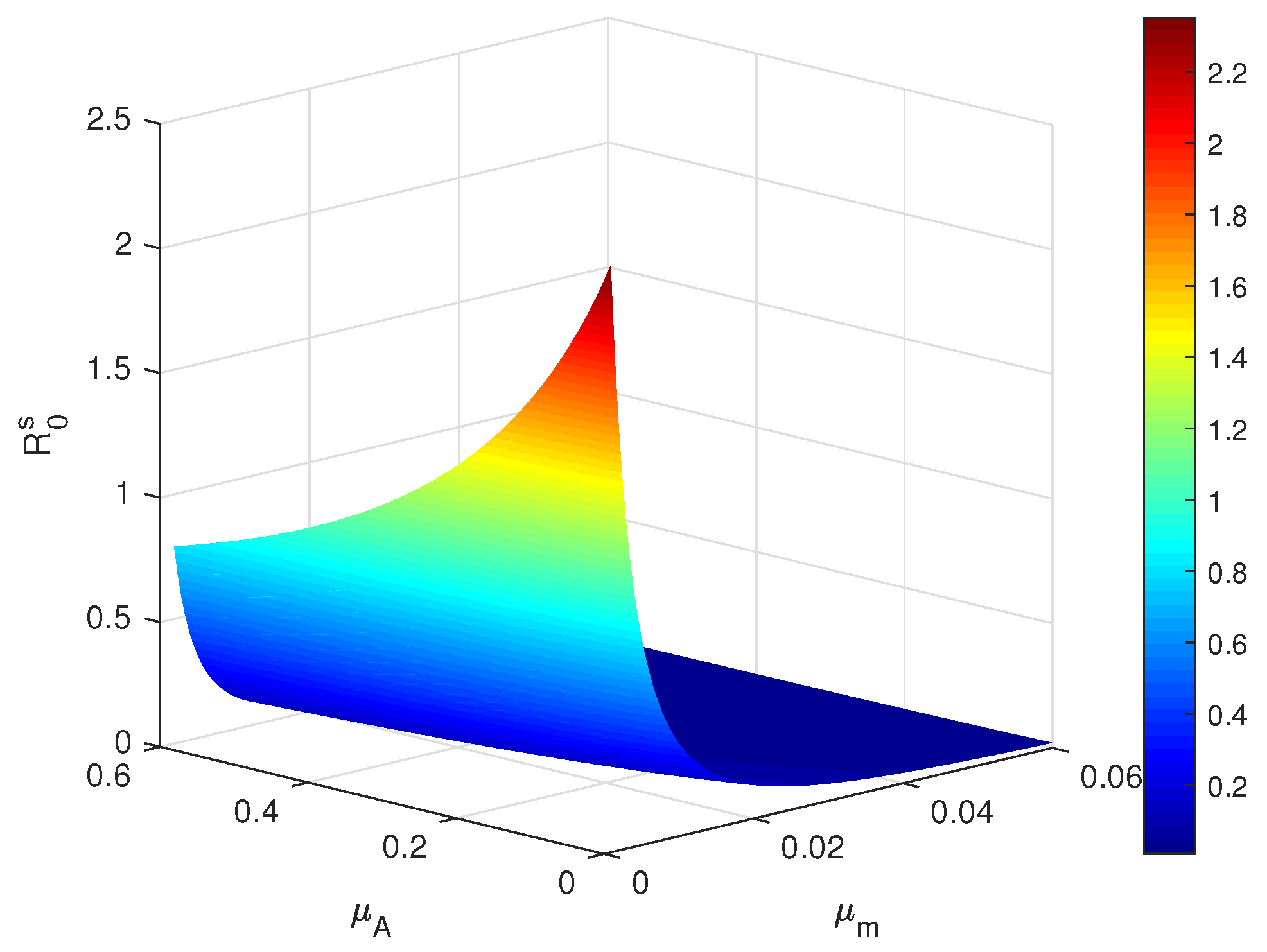
4.1. Sensitivity Analysis of Main Parameters

By numerical simulations, an extensive discussion on the sensitivity analysis of the main parameters is provided. In particular, the influences of the death rates of aquatic mosquitoes and adult mosquitoes on dengue transmission dynamics are mainly investigated. Let the intensities of the fluctuations be fixed as ${\sigma }_1=0.1,{\sigma }_2=0.1,{\sigma }_3=0.1,{\sigma }_4=0.001,{\sigma }_5=0.001.$ Based on the parameter ranges of Table 2, the main parameters with setting (I) are fixed in

Table 3. The main parameters for the numerical simulations to model (3).

Parameter	(I)		(II)		(III)		(IV)
	Value	Source	Value	Source	Value	Source	Value	Source
$\Gamma$	2000	Fitted	100	Fitted	2000	Fitted	1,800,000	Fitted
${\mu }_m$	(0, 0.06]	Fitted	0.05	[22]	0.03	[22]	${0.0149}^{\mathrm{a}}$	Fitted
							${0.1910}^{\mathrm{b}}$
b	$3.33\times {10}^{-6}$	Fitted	$1.0\times {10}^{-4}$	Fitted	$3.33\times {10}^{-6}$	Fitted	${7.36\times {10}^{-9}}^{\mathrm{c}}$	Fitted
$\Delta T$	0	Fitted	0	Fitted	0	Fitted	${20}^{\mathrm{d}}$	[2]
${\mu }_A$	(0.01, 0.6]	Fitted	0.01	[21]	0.01	[21]	0.01	[21]
$\gamma$	0.1428	[21]	0.1428	[21]	0.1428	[21]	0.1428	[21]
${\beta }_m$	0.75	[22]	0.6	[22]	0.75	[22]	0.7	[22]
${\beta }_h$	0.5	[22]	0.5	[22]	0.4	[22]	0.5	[22]
$\delta$	0.3	[26]	0.1	[26]	[0.1, 0.7]	Fitted	0.2	[26]
${\mu }_h$	$3.75\times {10}^{-5}$	[10]	$3.75\times {10}^{-5}$	[10]	$3.75\times {10}^{-5}$	[10]	${3.41\times {10}^{-5}}^{\mathrm{e}}$	[38]
$\Lambda$	0.56	Fitted	100	Fitted	0.56	Fitted	${282.5}^{\mathrm{f}}$	[38,54]

^a ${\mu }_m=0.0149$ was estimated by the least squares method for the period from 1 June to 11 September 2019. ^b ${\mu }_m=0.1910$ was estimated by the least squares method for the period from 12 September to 31 December 2019. ^c $b={\displaystyle \frac{0.061}{\mathrm{8,291,268}}}\approx 7.36\times {10}^{-9}$, where 0.061 was derived by the optimal fitting in Figure 5. ^d $\Delta T$ was taken as 20 days for Fuzhou dengue transmission because the mosquitoes took 8–12 days to be capable of spreading viruses to a new host, and the human beings with symptoms took 4–10 days after infection as reported in [2]. ^e Following [47], the formula of ${\mu }_h$ was written as ${\mu }_h={\displaystyle \frac{1}{\mathrm{LE}}}\times {\displaystyle \frac{1}{365}}$, where LE (life expectancy) was 80.41 years old in [38]. We then obtained ${\mu }_h={\displaystyle \frac{1}{80.41\times 365}}\approx 3.41\times {10}^{-5}$. ^f Following [47], the formula of $\Lambda$ was written as $\Lambda ={\displaystyle \frac{\mathrm{TPH}}{\mathrm{LE}}}\times {\displaystyle \frac{1}{365}}$, where TPH (total population size of human beings) was 8,291,268 in [54]. We then obtained $\Lambda ={\displaystyle \frac{\mathrm{8,291,268}}{80.41\times 365}}\approx 282.5$.

, the initial values with setting (I) are set in

Table 4. The initial values of the numerical simulations to model (3).

Variable	(I)	(II)	(III)	(IV)
$A\left(0\right)$	40,000	20,000	40,000	9,000,000
$S_m\left(0\right)$	20,000	20,000	20,000	10,000,000
$I_m\left(0\right)$	1,000	10	1,000	15
$S_h\left(0\right)$	15,000	15,596	15,000	8,291,266
$I_h\left(0\right)$	150	2	150	2
$R_h\left(0\right)$	0	0	0	0

, and the sensitivity analysis is carried out for ${\mathcal{R}}_0^s$ in Figure 1, which demonstrates the 3-dimensional image of ${\mathcal{R}}_0^s$ with respect to ${\mu }_A$ and ${\mu }_m$. Obviously, the value of ${\mathcal{R}}_0^s$ increases with the decrease in the death rates ${\mu }_A$ and ${\mu }_m$. Especially, the value of ${\mathcal{R}}_0^s$ declines fast with ${\mu }_m$ when the value of ${\mu }_A$ is fixed in Figure 1. The tendencies of infective mosquitoes and infective human beings are demonstrated when the changes in ${\mu }_A$ and ${\mu }_m$ are set in Figure 2. It is significant that the reductions for both $I_m$ and $I_h$ mainly depend on the increase in ${\mu }_m$.

4.2. Persistence in the Mean

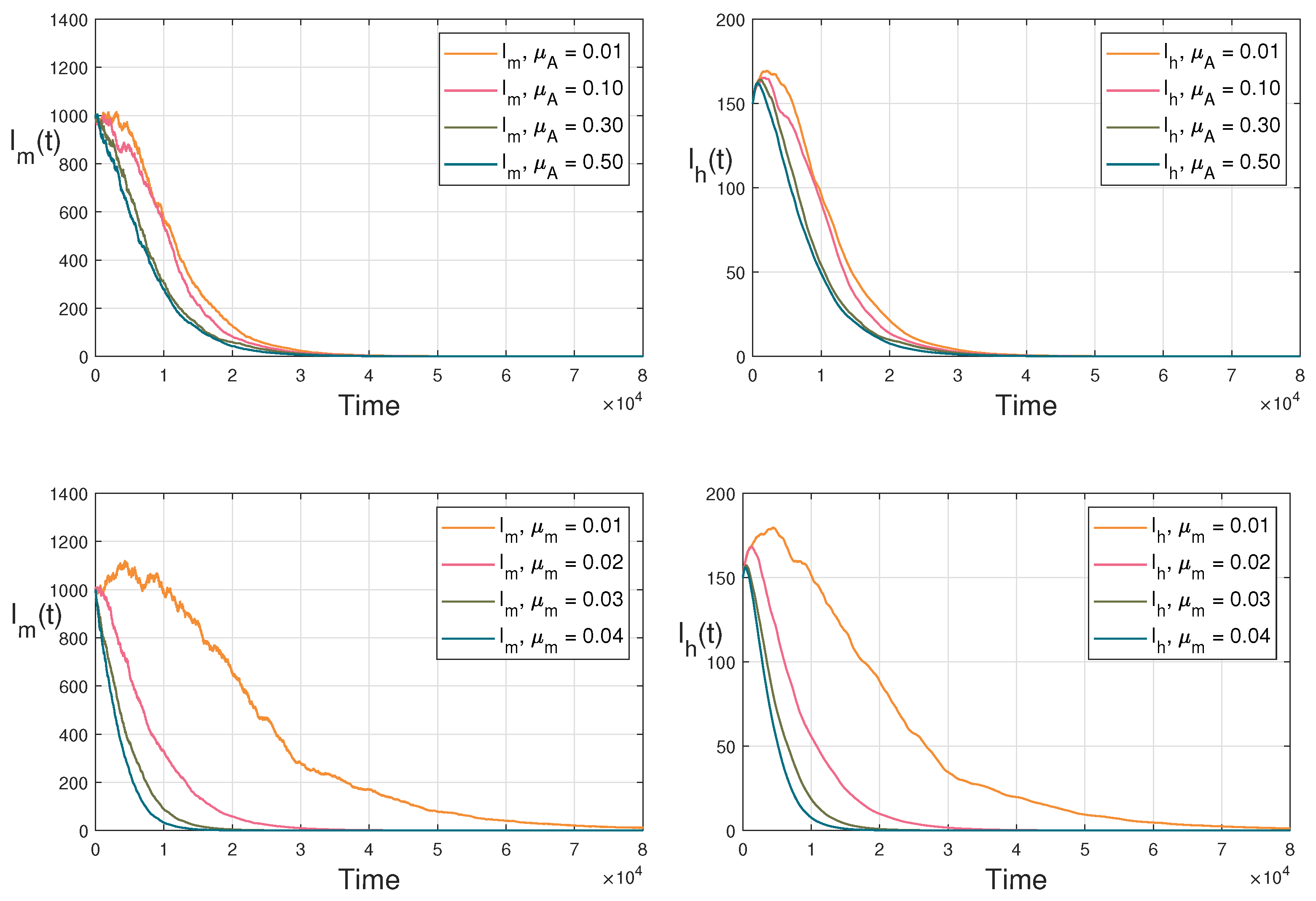
The PPTEM method for SDEs in [55,56] is adopted to organize the discretization equations of model (3). For further details, it is recommended to read the recent work [57]. For other approaches used in numerical simulations of SDEs, it is encouraged to consult [46,47] and references therein. Here, the numerical simulations of persistence in the mean are provided. The initial values with setting (II) of model (3) are presented in Table 4, and the main parameters with setting (II) are presented in Table 3. The intensities of the fluctuations are fixed as ${\sigma }_1=0.1$, ${\sigma }_2=0.1$, ${\sigma }_3=0.1$, ${\sigma }_4=0.001$, ${\sigma }_5=0.001$. The conditions of Theorem 2 are checked below:

$$\begin{array}{cc}\hfill & \sqrt[5]{{\mathcal{R}}_0^s}=4.3778>1,0.02=min\{{\mu }_A,{\mu }_m\}>max\{{\sigma }_1^2,{\sigma }_2^2,{\sigma }_3^2\}=0.01,\hfill \\ \hfill & 2/(73\times 365)=2{\mu }_h>max\{{\sigma }_4^2,{\sigma }_5^2\}=0.0001.\hfill \end{array}$$

Because the condition $\sqrt[5]{{\mathcal{R}}_0^s}=4.3778>1$ is equivalent to ${\mathcal{R}}_0^s>1$, by Section 3.3, model (3) has a unique stationary distribution. In other words, model (3) is ergodic. Consequently, the persistence in the mean of infective mosquitoes and infective human beings is illustrated on the left panel of Figure 3, and the probability density functions of model (3) around the quasi-equilibrium point $P^{*}$ with $A^{*}=909$, $S_m^{*}=988$, $I_m^{*}=830$, $S_h^{*}=2408$, $I_h^{*}=699$ are provided on the right side of Figure 3.

4.3. Extinction

The numerical simulations of the extinction of model (3) were performed using PPTEM. The initial values of setting (III) of model (3) were taken from Table 4, the main parameters of setting (III) are presented in Table 3, and the intensities of the fluctuations were set as ${\sigma }_1=0.1$, ${\sigma }_2=0.01$, ${\sigma }_3=0.01$, ${\sigma }_4=0.001$, ${\sigma }_5=0.001$. It is easy to check that $P_0$ with $A_0=2817$, $S_{m0}=65,728$, $I_{m0}=0$, $S_{h0}=15,000$, $I_{h0}=0$, and the conditions in Theorem 4 are checked as follows:

$$2min\{{\mu }_A,{\mu }_m\}>max\{{\sigma }_1^2,{\sigma }_2^2,{\sigma }_3^2\},2{\mu }_h>{\sigma }_4^2,\phi =-0.0007<0.$$

These simulation results show that the extinction occurs for a long period, which indicates that the population sizes of infective mosquitoes and infective human beings exponentially tend to zero as $\delta$ decreases on the left panel of Figure 4. Further, the parameter values are kept same, and if ${\beta }_h$ is taken as 0.5, $\delta$ is set as 0.1, then conditions of Theorem 4 are still valid with $P_0$ with $A_0=1818$, $S_{m0}=60,606$, $I_{m0}=0$, $S_{h0}=15,000$, $I_{h0}=0$, while the sign of $\phi$ changes as $\phi =0.0015>0$. The differences in the numerical simulations can be observed on the right side of Figure 4. The reduction in the maturity proportion of aquatic mosquitoes suppresses the number of infective human beings. But the effectiveness of this measure is limited as shown in Figure 4.

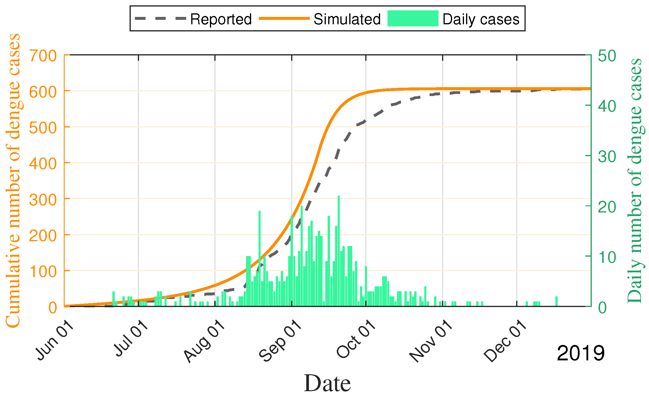
4.4. Application of Dengue in Fuzhou City

We used model (3) to investigate the 2019 dengue outbreak in Fuzhou City, and we adopted the surveillance data from 1 June to 31 December from Fujian CDC. According to the reports from [38,54], the total population size and the life expectancy of human beings of Fuzhou City in 2019 are 8,291,268 individuals and 80.41 years old, respectively, which then gives the following initial values while setting the human beings and related parameters to model (3):

$$S_h\left(0\right)=8,291,266,I_h\left(0\right)=2,R_h\left(0\right)=0,\Lambda ={\displaystyle \frac{8,291,268}{80.41\times 365}},{\mu }_h={\displaystyle \frac{1}{80.41\times 365}}.$$

Since the ratio for mosquito population to human population ranges from 0.53 to 2 in [58] and the number of daily average hatch of mosquitoes is from 0 to 2 in [22], we then assume the initial values with the setting of mosquitoes and related parameters as follows:

$$A\left(0\right)=9,000,000,S_m\left(0\right)=10,000,000,I_m\left(0\right)=15,\Gamma =1,800,000.$$

Let ${\sigma }_i=0$. Model (3) degenerates into the deterministic model (1). We fit model (1) on surveillance data to estimate parameters b and ${\mu }_m$ employing the major parameters listed in Table 3 and the least-squares method. Here, the awareness delay ($\Delta T$) is referred to as the time interval from the initial infection to the first confirmed diagnosis for the given infectious diseases [40].

Further, the curves for the cumulative number and daily number of dengue cases are shown in Figure 5. The main parameters with setting (IV) are collected without the fluctuations for the 2019 dengue outbreak. Since the number of infective human beings during the 2019 dengue outbreak was relatively small compared to the number of susceptible human beings, the changes in susceptible human beings introduce the randomness of human–mosquito contacts and the randomness of human behaviors. It is reasonable to incorporate the randomness into the 2019 dengue outbreak. Therefore, the effects of fluctuations of dengue were studied by setting ${\sigma }_1=0.01$, ${\sigma }_2=0.005$, ${\sigma }_3=0.005$, ${\sigma }_4=0.003$, ${\sigma }_5=0.003$ in Figure 6. The main findings indicate that the yellow curve is the mean of model (3) and the purple curves are the deviation to model (3) for 200 sample paths. Further, model (3) is valuable for the dynamic prediction of dengue.

5. Conclusions and Discussion

Since dengue is the most common mosquito-borne disease in human society and the population sizes of aquatic mosquitoes and adult mosquitoes affect the circulation, we establish a vector–host model with multiple stages and fluctuations for the transmission mechanism of dengue. We focus on the survival analysis of the vector–host model with the long-time dynamical properties in this paper.

In this study, we prove the existence and uniqueness of positive solutions of model (3) in Theorem 1 by contradiction. Then, we obtain the critical threshold ${\mathcal{R}}_0^s$ and prove that the population sizes of infective mosquitoes and infective human beings are persistent in the mean, when ${\mathcal{R}}_0^s>1$ is valid and conditions of Lemma 1 hold. By building the appropriate Lyapunov functions, we further demonstrate that when ${\mathcal{R}}_0^s>1$ holds in Theorem 3, model (3) has a unique stationary distribution. The corresponding simulations are performed by using the PPTEM method in Figure 3.

By using the comparison theorem, ergodic theorem, and some related stochastic analysis methods, we obtain the criteria of the extinction of model (3) in Theorem 4. Precisely, when $\phi <0$ is valid, $2min\{{\mu }_A,{\mu }_m\}>max\{{\sigma }_1^2,{\sigma }_2^2,{\sigma }_3^2\}$ and $2{\mu }_h>{\sigma }_4^2$ hold, and we find that the dengue model (3) undergoes eradication in the long run. The numerical simulations were carried out using the PPTEM method in Figure 4, of which the numerical simulations showed that the transfer proportion from aquatic mosquitoes to adult mosquitoes affects the infection scale of infective human beings with dengue virus. When the fluctuations disappeared, we conducted parameter estimations and numerical simulations of the 2019 dengue outbreak in Fuzhou City based on the surveillance data in Figure 5. When the intensities of the fluctuations were controlled, we employed model (3) to investigate the effects of fluctuations on the infection scale of dengue cases, and we further conclude that model (3) is feasible for the dynamic prediction of infection scale in Figure 6. We, therefore, suggest that policymakers pay more attention to the constant recruitment rates of aquatic mosquitoes, the maturity proportion of aquatic mosquitoes, and the death rate of aquatic mosquitoes before reasonable control measures are made. In the short-term, we will consider the optimal control of aquatic mosquitoes, the effects of time delay from aquatic mosquitoes to biting mosquitoes, and the periodic recruitment of dengue infection cases as the best possible investigations.

References

1. World Health Organization. Vector-Borne Disease-Key Facts. Available online: https://www.who.int/news-room/fact-sheets/detail/vector-borne-diseases (accessed on 9 May 2024).
2. World Health Organization. Dengue and Severe Dengue-Key Facts. Available online: https://www.who.int/news-room/fact-sheets/detail/dengue-and-severe-dengue (accessed on 9 May 2024).
3. Wilder-Smith, A.; Ooi, E.E.; Horstick, O.; Wills, B. Dengue. Lancet 2019, 393, 350–363. [Google Scholar] [CrossRef]
4. Bhatt, S.; Gething, P.W.; Brady, O.J.; Messina, J.P.; Farlow, A.W.; Moyes, C.L.; Drake, J.M.; Brownstein, J.S.; Hoen, A.G.; Sankoh, O.; et al. The global distribution and burden of dengue. Nature 2013, 496, 504–507. [Google Scholar] [CrossRef] [PubMed]
5. Kraemer, M.U.G.; Reiner, R.C.; Brady, O.J.; Messina, J.P.; Gilbert, M.; Pigott, D.M.; Yi, D.; Johnson, K.; Earl, L.; Marczak, L.B.; et al. Past and future spread of the arbovirus vectors Aedes aegypti and Aedes albopictus. Nat. Microbiol. 2019, 4, 854–863. [Google Scholar] [CrossRef] [PubMed]
6. Colón-González, F.J.; Sewe, M.O.; Tompkins, A.M.; Sjödin, H.; Casallas, A.; Rocklöv, J.; Caminade, C.; Lowe, R. Projecting the risk of mosquito-borne diseases in a warmer and more populated world: A multi-model, multi-scenario intercomparison modelling study. Lancet Planet. Health 2021, 5, e404–e414. [Google Scholar] [CrossRef]
7. Reiter, P.; Newton, E.A.C. A model of the transmission of dengue fever with an evaluation of the impact of Ultra-Low Volume (ULV) insecticide applications on dengue epidemics. Am. J. Trop. Med. Hyg. 1992, 47, 709–720. [Google Scholar]
8. Lotka, A.J. Contribution to the analysis of malaria epidemiology. II. General part (continued). Comparison of two formulae given by Sir Ronald Ross. Am. J. Epidemiol. 1923, 3, 38–45. [Google Scholar] [CrossRef]
9. Jan, R.; Xiao, Y. Effect of partial immunity on transmission dynamics of dengue disease with optimal control. Math. Methods Appl. Sci. 2019, 42, 1967–1983. [Google Scholar] [CrossRef]
10. Xue, L.; Jin, X.; Zhu, H. Assessing the impact of serostatus-dependent immunization on mitigating the spread of dengue virus. J. Math. Biol. 2023, 87, 5. [Google Scholar] [CrossRef]
11. Asamoah, J.K.K.; Yankson, E.; Okyere, E.; Sun, G.; Jin, Z.; Jan, R.; Fatmawati. Optimal control and cost-effectiveness analysis for dengue fever model with asymptomatic and partial immune individuals. Results. Phys. 2021, 31, 104919. [Google Scholar] [CrossRef]
12. Xue, L.; Ren, X.; Magpantay, F.; Sun, W.; Zhu, H. Optimal control of mitigation strategies for dengue virus transmission. Bull. Math. Biol. 2021, 83, 8. [Google Scholar] [CrossRef]
13. Bian, G.; Xu, Y.; Lu, P.; Xie, Y.; Xi, Z. The endosymbiotic bacterium wolbachia induces resistance to dengue v irus in Aedes aegypti. PLoS Pathog. 2010, 6, e1000833. [Google Scholar] [CrossRef] [PubMed]
14. Zhang, X.; Tang, S.; Cheke, R.A. Models to assess how best to replace dengue virus vectors with Wolbachia-infected mosquito populations. Math. Biosci. 2015, 269, 164–177. [Google Scholar] [CrossRef]
15. Zhang, Z.; Chang, L.; Huang, Q.; Yan, R.; Zheng, B. A mosquito population suppression model with a saturated Wolbachia release strategy in seasonal succession. J. Math. Biol. 2023, 86, 51. [Google Scholar] [CrossRef] [PubMed]
16. Li, C.; Wang, Z.; Yan, Y.; Qu, Y.; Hou, L.; Li, Y.; Chu, C.; Woodward, A.; Schikowski, T.; Saldiva, P.H.N.; et al. Association between hydrological conditions and dengue fever incidence in coastal southeastern China from 2013 to 2019. JAMA Netw. Open. 2023, 6, e2249440. [Google Scholar] [CrossRef] [PubMed]
17. Liu, Y.; Wang, X.; Tang, S.; Cheke, R.A. The relative importance of key meteorological factors affecting numbers of mosquito vectors of dengue fever. PLoS Neglected Trop. Dis. 2023, 17, e0011247. [Google Scholar] [CrossRef] [PubMed]
18. Abdelrazec, A.; Gumel, A.B. Mathematical assessment of the role of temperature and rainfall on mosquito population dynamics. J. Math. Biol. 2017, 74, 1351–1395. [Google Scholar] [CrossRef] [PubMed]
19. Adams, B.; Boots, M. How important is vertical transmission in mosquitoes for the persistence of dengue? Insights from a mathematical model. Epidemics 2010, 2, 1–10. [Google Scholar] [CrossRef] [PubMed]
20. Amaku, M.; Coutinho, F.A.B.; Raimundo, S.M.; Lopez, L.F.; Burattini, M.N.; Massad, E. A comparative yanalysis of the relative efficacy of vector-control strategies against dengue fever. Bull. Math. Biol. 2014, 76, 697–717. [Google Scholar] [CrossRef] [PubMed]
21. Zou, L.; Chen, J.; Feng, X.; Ruan, S. Analysis of a dengue model with vertical transmission and application to the 2014 dengue outbreak in Guangdong Province, China. Bull. Math. Biol. 2018, 80, 2633–2651. [Google Scholar] [CrossRef]
22. Li, M.; Sun, G.; Yakob, L.; Zhu, H.; Jin, Z.; Zhang, W. The driving force for 2014 dengue outbreak in Guangdong, China. PLoS ONE 2016, 11, e0166211. [Google Scholar] [CrossRef]
23. Defterli, O. Comparative analysis of fractional order dengue model with temperature effect via singular and non-singular operators. Chaos Solitons Fractals 2021, 144, 110654. [Google Scholar] [CrossRef]
24. Hamdan, N.I.; Kilicman, A. Mathematical modelling of dengue transmission with intervention strategies using fractional derivatives. Bull. Math. Biol. 2022, 84, 138. [Google Scholar] [CrossRef] [PubMed]
25. Cai, L.; Li, X.; Fang, B.; Ruan, S. Global properties of vector-host disease models with time delays. J. Math. Biol. 2017, 74, 1397–1423. [Google Scholar] [CrossRef] [PubMed]
26. Abdelrazec, A.; Bélair, J.; Shan, C.; Zhu, H. Modeling the spread and control of dengue with limited public health resources. Math. Biosci. 2016, 271, 136–145. [Google Scholar] [CrossRef] [PubMed]
27. Hajji, M.E.; Aloufi, M.F.S.; Alharbi, M.H. Influence of seasonality on Zika virus transmission. AIMS Math. 2024, 9, 19361–19384. [Google Scholar] [CrossRef]
28. Otero, M.; Solari, H.G. Stochastic eco-epidemiological model of dengue disease transmission by Aedes aegypti mosquito. Math. Biosci. 2010, 223, 32–46. [Google Scholar] [CrossRef] [PubMed]
29. Jovanović, M.; Krstić, M. Stochastically perturbed vector-borne disease models with direct transmission. Appl. Math. Model. 2012, 36, 5214–5228. [Google Scholar] [CrossRef]
30. Britton, T.; Traoré, A. A stochastic vector-borne epidemic model: Quasi-stationarity and extinction. Math. Biosci. 2017, 289, 89–95. [Google Scholar] [CrossRef]
31. Liu, Q.; Jiang, D.; Hayat, T.; Alsaedi, A. Stationary distribution and extinction of a stochastic dengue epidemic model. J. Frankl. Inst. 2018, 355, 8891–8914. [Google Scholar] [CrossRef]
32. Sun, W.; Xue, L.; Yan, X. Stability of a dengue epidemic model with independent stochastic perturbations. J. Math. Anal. Appl. 2018, 468, 998–1017. [Google Scholar] [CrossRef]
33. Liu, P.; Din, A.; Zenab. Impact of information intervention on stochastic dengue epidemic model. Alex. Eng. J. 2021, 60, 5725–5739. [Google Scholar] [CrossRef]
34. Guo, M.; Hu, L.; Nie, L. Stochastic dynamics of the transmission of dengue fever virus between mosquitoes and humans. Int. J. Biomath. 2021, 14, 2150062. [Google Scholar] [CrossRef]
35. Kiouach, D.; El-idrissi, S.E.A.; Sabbar, Y. A novel mathematical analysis and threshold reinforcement of a stochastic dengue epidemic model with Lévy jumps. Commun. Nonlinear Sci. Numer. Simul. 2023, 119, 107092. [Google Scholar] [CrossRef]
36. Valdez, L.D.; Sibona, G.J.; Diaz, L.A.; Contigiani, M.S.; Condat, C.A. Effects of rainfall on Culex mosquito population dynamics. J. Theor. Biol. 2017, 421, 28–38. [Google Scholar] [CrossRef]
37. Wang, X.; Tang, S.; Wu, J.; Xiao, Y.; Cheke, R.A. A combination of climatic conditions determines major within-season dengue outbreaks in Guangdong Province, China. Parasites Vectors 2019, 12, 45. [Google Scholar] [CrossRef] [PubMed]
38. Fuzhou City Bureau of Statistics. Available online: https://tjj.fuzhou.gov.cn/zz/zwgk/tjzl/tjxx/202111/t20211115_4242144.htm (accessed on 9 May 2024).
39. Van Den Driessche, P.; Watmough, J. Reproduction numbers and sub-threshold endemic equilibria for compartmental models of disease transmission. Math. Biosci. 2002, 180, 29–48. [Google Scholar] [CrossRef]
40. Lan, X.; Chen, G.; Zhou, R.; Zheng, K.; Cai, S.; Wei, F.; Jin, Z.; Mao, X. An SEIHR model with age group and social contact for analysis of Fuzhou COVID-19 large wave. Infect. Dis. Model. 2024, 9, 728–743. [Google Scholar] [CrossRef] [PubMed]
41. Zhao, Y.; Jiang, D. The threshold of a stochastic SIS epidemic model with vaccination. Appl. Math. Comput. 2014, 243, 718–727. [Google Scholar] [CrossRef]
42. Mao, X.; Marion, G.; Renshaw, E. Environmental Brownian noise suppresses explosions in population dynamics. Stoch. Process Appl. 2002, 97, 95–110. [Google Scholar] [CrossRef]
43. Wei, F.; Xue, R. Stability and extinction of SEIR epidemic models with generalized nonlinear incidence. Math. Comput. Simul. 2020, 170, 1–15. [Google Scholar] [CrossRef]
44. Mao, X. Stochastic Differential Equations and Applications; Horwood Publishing Limited: Chichester, UK, 2007. [Google Scholar]
45. Zhao, Y.; Jiang, D. Dynamics of stochastically perturbed SIS epidemic model with vaccination. Abstr. Appl. Anal. 2013, 2013, 1–12. [Google Scholar] [CrossRef]
46. Li, D.; Wei, F.; Mao, X. Stationary distribution and density function of a stochastic SVIR epidemic model. J. Frankl. Inst. 2022, 359, 9422–9449. [Google Scholar] [CrossRef]
47. Li, W.; Cai, S.; Zhai, X.; Ou, J.; Zheng, K.; Wei, F.; Mao, X. Transmission dynamics of symptom-dependent HIV/AIDS models. Math. Biosci. Eng. 2024, 21, 1819–1843. [Google Scholar] [CrossRef]
48. Wei, F.; Jiang, H.; Zhu, Q. Dynamical behaviors of a heroin population model with standard incidence rates between distinct patches. J. Frankl. Inst. 2021, 358, 4994–5013. [Google Scholar] [CrossRef]
49. Ikeda, N.; Watanabe, S. A comparison theorem for solutions of stochastic differential equations and its applications. Osaka J. Math. 1977, 14, 619–633. [Google Scholar]
50. Peng, S.; Zhu, X. Necessary and sufficient condition for comparison theorem of 1-dimensional stochastic differential equations. Stoch. Process Appl. 2006, 116, 370–380. [Google Scholar] [CrossRef]
51. Wei, F.; Wang, C. Survival analysis of a single-species population model with fluctuations and migrations between patches. Appl. Math. Model. 2020, 81, 113–127. [Google Scholar] [CrossRef]
52. Kutoyants, Y.A. Statistical Inference for Ergodic Diffusion Processes; Springer: London, UK, 2004. [Google Scholar]
53. Berman, A.; Plemmons, R.J. Nonnegative Matrices in the Mathematical Sciences; SIAM Publisher: Philadelphia, PA, USA, 1994. [Google Scholar]
54. Fuzhou City Bureau of Statistics. Available online: https://tjj.fuzhou.gov.cn/zz/zwgk/tjzl/ndbg/202105/t20210524_4105019.htm (accessed on 9 May 2024).
55. Mao, X.; Wei, F.; Wiriyakraikul, T. Positivity preserving truncated Euler-Maruyama Method for stochastic Lotka-Volterra competition model. J. Comput. Appl. Math. 2021, 394, 113566. [Google Scholar] [CrossRef]
56. Cai, Y.; Mao, X.; Wei, F. An advanced numerical scheme for multi-dimensional stochastic Kolmogorov equations with superlinear coefficients. J. Comput. Appl. Math. 2024, 437, 115472. [Google Scholar] [CrossRef]
57. Zhai, X.; Li, W.; Wei, F.; Mao, X. Dynamics of an HIV/AIDS transmission model with protection awareness and fluctuations. Chaos Solitons Fractals 2023, 169, 113224. [Google Scholar] [CrossRef]
58. Wang, L.; Teng, Z.; Ji, C.; Feng, X.; Wang, K. Dynamical behaviors of a stochastic malaria model: A case study for Yunnan, China. Phys. Stat. Mech. Appl. 2019, 521, 435–454. [Google Scholar] [CrossRef]
Figure 1. Plot of the critical threshold R 0 s in terms of μ A and μ m .
Mathematics 12 02491 g001
Figure 2. The tendencies of infective mosquitoes and infective human beings when μ A and μ m change in their values.
Mathematics 12 02491 g002
Figure 3. The persistence in the mean and stationary distribution of A, S m , I m , S h , I h of model (3).
Mathematics 12 02491 g003
Figure 4. Extinctions of infective mosquito population and infective human population with the exponential rates as δ decreases.
Mathematics 12 02491 g004
Figure 5. Cumulative number and daily number of the 2019 dengue outbreak from 1 June to 31 December in Fuzhou City.
Mathematics 12 02491 g005
Figure 6. Cumulative number of the 2019 dengue outbreak with fluctuations from 1 June to 31 December in Fuzhou City.
Mathematics 12 02491 g006