Abstract
A model for generating synthetic time series data using pre-trained large language models is proposed. Starting with the Google T5-base model, which employs an encoder–decoder transformer architecture, the model underwent pre-training on diverse datasets. It was then fine-tuned using the QLoRA technique, which reduces computational complexity by quantizing weight parameters. The process involves the tokenization of time series data through mean scaling and quantization. The performance of the model was evaluated with fidelity, utility, and privacy metrics, showing improvements in fidelity and utility but a trade-off with reduced privacy. The proposed model offers a foundation for decision intelligence systems.
Keywords:
transformer architecture; large language models; synthetic data; time series; decision intelligence MSC:
62M10; 68T10
1. Introduction
In a phase of rapid development, machine learning (ML) methods become able to help businesses solve problems that are too hard or time-consuming for people. While technical people understand how computers work and how to use them to their advantage, business executives or decision-makers have limited understanding of how to program computers to execute the needed tasks. Their preferred interaction method with a computer is by writing in the natural language. Decision Intelligence [1] represents a methodology that starts from the decision objective and creates actionable insights that help in making data-driven decisions. This solves the problem for business executives and gives them the required information needed to make better decisions.
Making a decision intelligence system requires using an ML model. For example, in forecasting the revenue of a business, an artificial neural network can be used to determine future revenue based on past data. The models rely on having a significant amount of data already available for forecasting. One problem arises when the data are either unavailable or insufficient based on the forecast length. Having access to enough real-world data is a challenge in itself; collecting and storing data can be expensive or pose privacy risks. Even if they are available, they are not always structured or continuous and introduce the necessity to be preprocessed to obtain useful information. Another problem is data privacy. In some domains, client data have privacy requirements and cannot be explicitly used in machine learning models. Therefore, data need to be anonymized and reconstructed to meet privacy requirements.
For businesses, data are usually represented in a tabular format. The rows are the observations taken in the respective field, and the columns display the attributes of those observations. An important component in the data that most organizations use are the time index. This leads to creating synthetic time series for companies that want to forecast different scenarios or create historical data that are not available for the current models [2]. Having the time component adds complexity to the model, as it should not be generated randomly and needs to keep similar statistical properties. As used in decision intelligence tools, time series are a subtype of tabular data. This work focused on time series, which can represent the sales values of products, the number of products sold, or the availability of supply chain providers.
A solution to these problems is creating synthetic data (SD) that have similar statistical properties to the real ones and testing models in different scenarios. Two cases will be used for their existent data: extension and reconstruction. There are different types of SD based on the objective of the system. It can be generated from real data, where a model captures the distributions and structure and is used in extension and reconstruction. Another way is without real data, where it can be generated by an existing model of a process, by generic assumptions of a specific phenomenon or by using the analyst’s background knowledge and different simulations [3]. The present work focused on generating data from existing data. There are multiple advantages to creating data. It is more cost-efficient than collecting, storing, and managing real data. It can help with privacy regulation and protect sensitive customer information; it offers better scalability by generating datasets as large as needed. Another advantage is the reduction of bias and the increase in diversity by generating different scenarios. SD have use cases in almost all domains, including generating insights, understanding the topic, or forecasting different scenarios [4].
The main contribution of this work is defining a model for generating synthetic time series datasets based on pre-trained large language models (LLMs), which can then be used for training machine learning models. While there are multiple methods for generating data, the latest research is focused on models based on the transformer architecture. This can help in situations where there are not enough data available or privacy restrictions apply. For example, privacy risks may appear when real datasets exist but cannot be publicly shared.
The rest of the paper is structured as follows. Section 2 includes the related research in the domain of tabular and time series synthetic data generation. Section 3 includes the proposed model architecture for generating the synthetic data. Section 4 contains the evaluation metrics and experiments performed to assess the synthetic data. The last section contains the conclusions and future work to improve the model.
2. Related Work
GAN and VAE. Generating SD is an area in current development. While most of the models include generative adversarial networks (GANs) [5] and variational autoencoders (VAEs) [6], current research focuses on transformers [7] and large language models. Multiple GAN models have been proposed for tabular data, e.g., in [8,9], which shows that a universal model for generating synthetic data does not exist, and there is a need for improvements in this area. Focusing on time series data, MedGAN [10] was used to generate realistic synthetic patient records. It combines the autoencoder and GAN to generate high-dimensional discrete variables, uses mini-batch averaging to avoid mode collapse, and increases learning efficiency by using shortcut connections and batch normalization. The results demonstrate feasibility by achieving comparable performance with real data and showing limited privacy risk. Good synthetic data generators (SDGs) should preserve the temporal dynamic when using time series data. Newly generated sequences should keep the original relationship between variables in time, as used in the TimeGAN model [11]. The model combines the control of supervised learning with the flexibility of the unsupervised paradigm. The main idea is to use two autoencoding components (an embedding function and the recovery function) trained jointly with the adversarial components (the sequence generator and discriminator) in a way that the model simultaneously learns to encode features, generates representations, and iterates across time. It demonstrates improvements over the state-of-the-art models on multiple datasets.
Challenges. There are multiple challenges in training GANs [12], which open the space for other methods or improvements. The lack of convergence affects the training of the model when the parameters oscillate and never reach stability. This becomes an issue when choosing the initial values. Mode collapse happens when the generator cannot produce more varieties of samples. Another problem, the vanishing gradient, appears when a discriminator is so efficient that the generator can no longer learn. When using time series data, one of the disadvantages of GANs is the difficulty of capturing long-term temporal dynamics. DoppelGANger (DG) [13] improves the model by using batch generation. By using auto-normalization, it tackles the mode collapse by normalizing each time series signal individually. To map the relationship between measurements and attributes, it uses an auxiliary discriminator that verifies only the attributes. The experiments show that DG achieves a significant improvement in fidelity over baseline models. It also enables what-if analysis when users can create changes in the underlying system to generate the corresponding results, which is useful in decision intelligence systems.
Transformers. Following the increase in the popularity of LLMs, recent research has focused on using transformers to generate synthetic tabular data. The studies presented next improve or propose new methods. Generating tabular data requires keeping the relations between columns. There are multiple models based on GPT2 that take advantage of the generative nature of the transformer. REaLTABFormer generates non-relational data and then creates the relational dataset conditioned on the initial table using a sequence-to-sequence model [14]. It achieves state-of-the-art results on prediction tasks and captures relational structure better than a baseline model. GReaT [15] generates tabular data by conditioning on any subset of features, and the remaining features are sampled without additional overhead. This is demonstrated in the tests performed on multiple real-world and synthetic datasets. A model based on BERT [16,17], a pre-trained LLM that is used in tasks such as sentiment analysis, can also be used to generate synthetic data. There are proposals using NeMo LLM for generating synthetic time series data [18], although there are no results comparing it with other models for this particular task. BERT is used in TabFormer, which relies on two architectures for tabular time series: one for learning representations that are analogous to BERT, which can be pre-trained end-to-end and used in downstream tasks, and another with GPT, which can be used to generate realistic synthetic tabular sequences [19]. Working with LLMs for data manipulation tasks (such as query, insert, modify, delete operations, question answering, or data analysis) is not an easy task on traditional pre-trained models. TableGPT proposes a framework that allows LLMs to better understand and work on tables using external functional commands [20]. TabText is a framework that converts the table into natural language phrases to be used in LLMs as input [21]. While the majority of transformer models are made for tabular data, there are also methods proposed for time series data that leverage the relations between time elements. TTS-GAN modifies the GAN architecture by using transformers for the generator and discriminator instead of neural networks [22]. TsT-GAN uses unsupervised masked modeling to produce synthetic sequences that capture both the global distribution and the conditional time-series dynamics [23]. CEHR-GPT uses GPT and captures the temporal dependencies in patient histories, which has proved useful in generating EHR patient data [24].
Tokenization. Tokenizing time-series data for transformer models is an important task in fine-tuning LLMs. Multiple versions are proposed in [25,26]. Tokenizers are used by LLMs in their input to split the text into smaller chunks. Tokenizers may find it difficult to understand context and repeating patterns because they are not meant to represent numerical values. They can also perceive consecutive values as distinct tokens and ignore the temporal relations between them. While traditional LLMs use tokenizers that split numbers in different ways, LLaMA uses a tokenizer that splits numbers into individual digits, which makes it more efficient in handling integers and floating-point numbers. There are methods that are explored in time series forecasting tasks in [27]. Analyzing the impact of different tokenization methods on model performance is important when choosing the best one. A tokenization method that uses an encoder–decoder architecture shows a significant improvement in classification and forecasting tasks [28]. It is also important how numbers are tokenized. Adding spaces to create one token per digit improves the performance on GPT-3 but decreases the performance on LLaMA-2, which tokenizes digits individually [29]. Another method utilizes the frequency spectrum as a common dictionary for tokenizing time series sequences, which converts single time series into frequency units with weights. Applied to a transformer’s architecture, it outperforms the state-of-the-art transformer models [30]. The results show that using specialized tokenizers for TS data can increase the performance of the LLM if applied to the right LLM. The advancement in handling time series data could unlock a wide range of possibilities, which includes modality switching and time series question answering.
Evaluation. There are multiple ways to evaluate synthetic data, which makes comparing multiple models difficult. There are applications where time series data pose challenges for SDGs. Financial time series data have limited availability and an irregular nature [31], which makes it harder for an SDG to get good results. SD can be evaluated based on fidelity, utility, and privacy. Achieving a trade-off between these is necessary, depending on the goals. Synthcity offers a framework for benchmarking synthetic data to easily compare multiple models [32]. There is also the question of how useful are the synthetic data compared with real-world data. Among the members of the scientific community, there is still no consensus on its usefulness, as analyzed in [33]. On the task of boosting ML models, there are marginal improvements in using synthetic data in training ML models. A problem also exists in the metrics of evaluating SDGs, which exposes the lack of standardization of metrics in the research literature. Only the widespread use of SD can improve the applications in different domains.
3. The Proposed Model
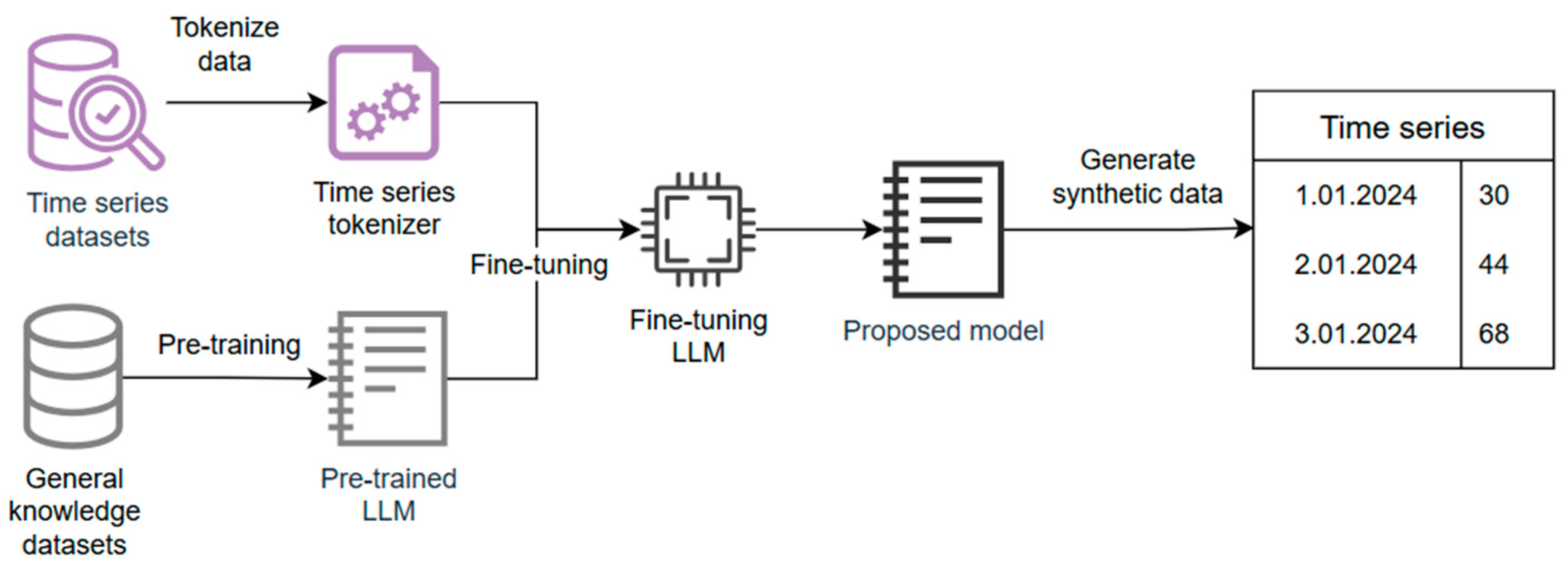
A model for generating synthetic time series data is proposed. The model starts from the development of pre-trained LLMs, which are a specific type of transformer trained on large amounts of data. An LLM learns to predict the next word given the input sequence of words and the context of these words, which makes it a good choice for SDG. There are multiple steps needed for creating the model, as seen in Figure 1.
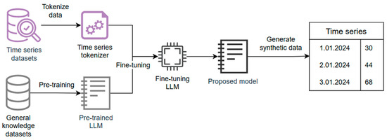
Figure 1.
The proposed synthetic generator model architecture.
3.1. Pre-Trained LLM
The initial step is model pre-training, where the model is fed with an extensive dataset that contains different articles, books, websites, or others. Using unsupervised learning, the model learns to predict the next sequence of words given the input. The Google T5-base [34] pre-trained model was chosen as a base model with 220 million parameters. T5 uses an encoder–decoder transformer architecture, which relies on the attention mechanism to process sequences of text. The encoder processes the input and converts it into a set of hidden representations, while the decoder takes the representations and generates the output text. It uses the sentencepiece [35] tokenizer, which handles diverse and complex linguistic inputs effectively. After pre-training, the model learns general knowledge to determine the output of basic questions.
3.2. Fine-Tuning
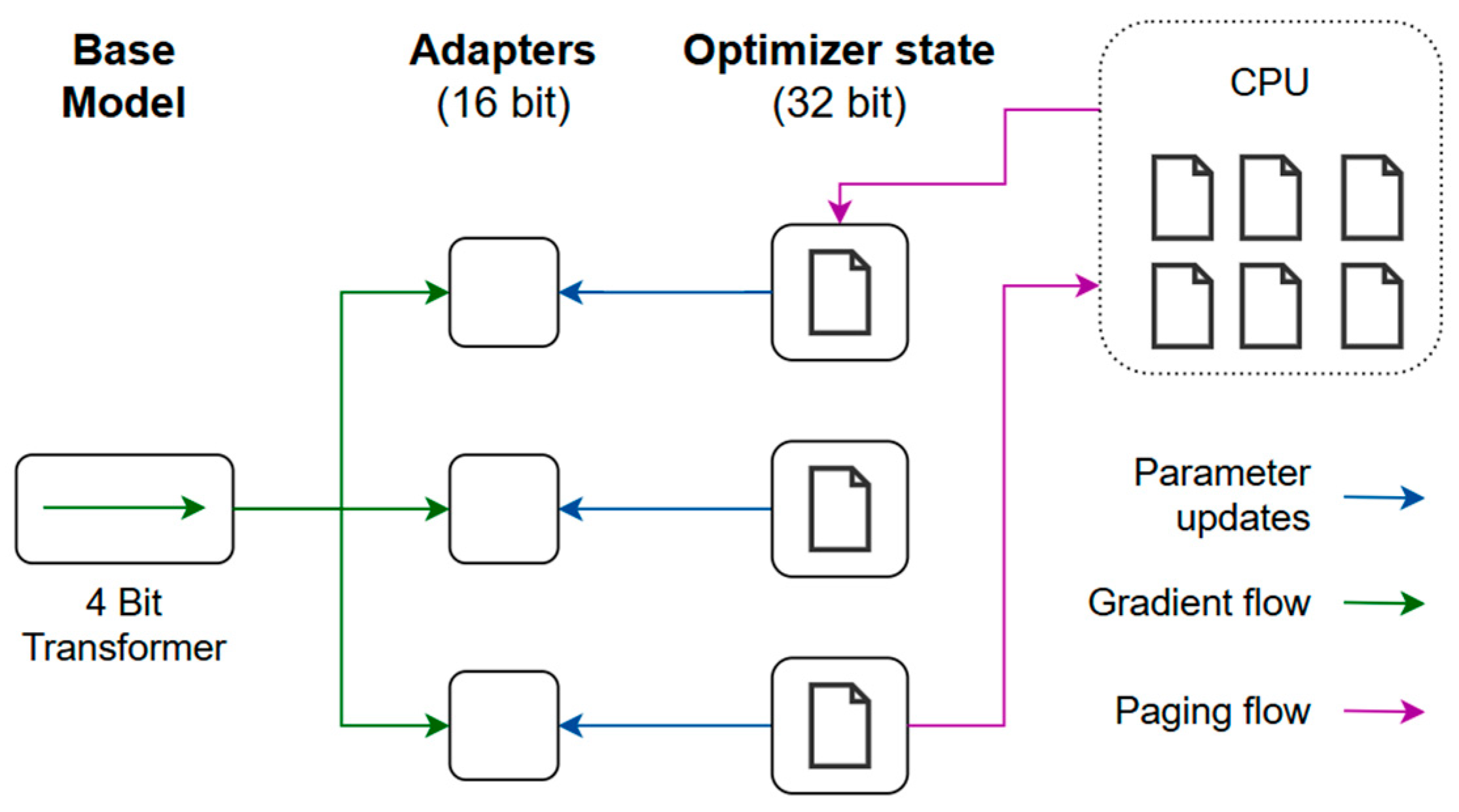
The second step is fine-tuning, which is the process of transforming the general-purpose model into a specialized one. Smaller and more specific datasets are fed into the model to improve the performance on a specific domain. The time dependency adds complexity to the model, which makes it necessary to improve the input tokenizer to handle time series data. A challenge in fine-tuning is the significant amount of time and storage capacity necessary to handle the computational load. There are multiple fine-tuning methods that can be used. Prefix tuning involves adding trainable prefix tokens to the input sequences to allow the model to adapt to new tasks without modifying the original weights of the model. It is very good as a cost-saving measure, but the limitation is that it may not perform well in capturing specific task features. Distillation involves training a smaller model that replicates the behavior of the larger model, but this may require careful tuning. The concept of parameter-efficient fine-tuning is introduced to overcome these limitations, which works by reducing the number of trainable parameters in a neural network. The Low-Rank Adaptation of Large Language Models (LoRA) technique introduces trainable rank decomposition matrices into each layer of the transformer. This technique shows that the new parameters introduced are merged back into the model without increasing the total number of parameters. The fine-tuning method used is QLoRA (Quantized LoRA), shown in Figure 2, which is an extended version of LoRA that quantizes the precision of weight parameters to 4 bit precision instead of 32 bit. This reduces memory utilization, making it able to run on consumer GPUs [36]. Using QLoRA, the model was trained with a learning rate of 2.5 · 10−5 over 500 iterations using the Adam optimizer. The loss function is cross entropy. QLoRA uses the rank 32, which controls the number of parameters trained, and a scaling factor alpha of 64.
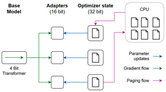
Figure 2.
QLoRA fine-tuning method (adapted from [36]).
3.3. Tokenization
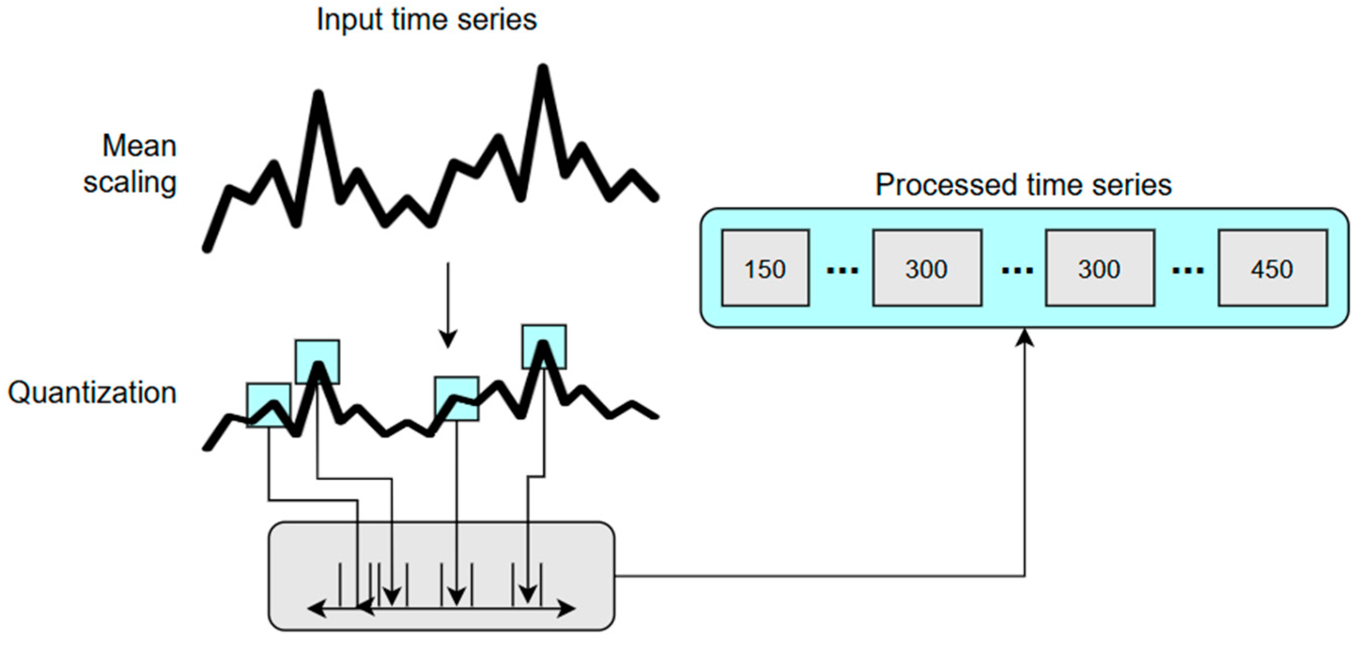
Dividing the input text into smaller units is an important task in training LLMs. Depending on the technique, tokens can consist of a wide range of segments, including characters, words, sub-words, or symbols. The tokenizers usually struggle in multiple cases, such as case sensitivity, trailing whitespace, digit chunking, integers, floating-point numbers, arithmetic reasoning, and model-specific behavior. To be used in fine-tuning the LLM as input, the time series sequence is converted into a sequence of tokens, as shown in Figure 3, using scaling and quantization [37]. This allows the model to handle numerical data as a language model would handle text. The first step is applying mean scaling [38] to the time series to normalize the data. Considering a time series as , where the C time steps are the historical context and H steps are the forecast horizon, the scaling formula is defined in Equation (1), where the scale is . This step ensures that the values are on a similar scale, which is important for the model to process them effectively. The second step is to quantize the scaled values to a fixed number of discrete tokens. This reduces the granularity of the data by mapping the original values to a smaller set of representative values or levels, as defined in Equation (2). Considering bin centers and edges , , where , the quantization function is and the dequantization function is . There are multiple ways of determining the number of bins B [39], for example, quantile binning, which is data-dependent, and uniform binning. In the proposed model, uniform binning is chosen. It uniformly selects the bin centers within an interval . The number of bins chosen for the experimental studies is B = 4094, and this can be changed depending on the input dataset and its frequency to capture the cycles.
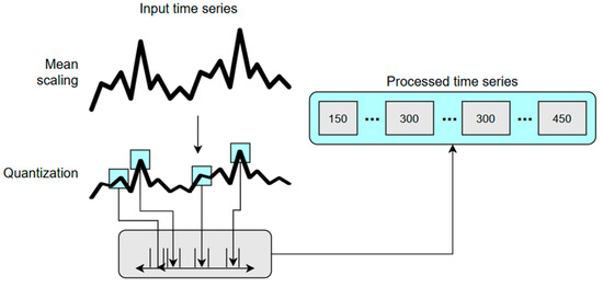
Figure 3.
The time series data tokenization (adapted from [37]).
3.4. Inference
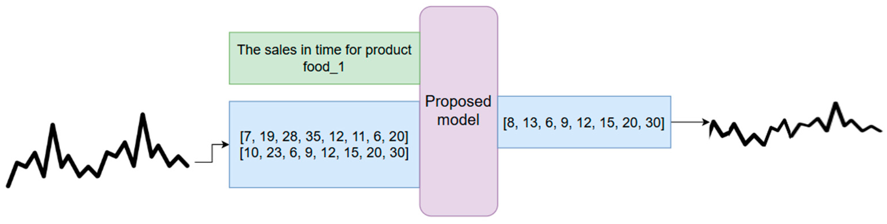
The third step is inference to generate new synthetic datasets based on some rules or existing data. In the context of an LLM, the inference is the capacity to produce predictions or answers corresponding with the input and context that it has been given. The model responds to prompts with relevant and appropriate responses by using its knowledge. Figure 4 represents the process of generating output text based on input context and existing time series. An example of a time series and the description of the data are used as the input. The model outputs the synthetic time series. The tokens generated by the models are mapped using the dequantization function from Equation (2) to the real values by applying the inverse scaling transformation. To handle long-term dependencies in time series data, the transformer uses the self-attention mechanism, which allows each time step to consider all other time steps in the sequence. Positional encodings are added to the input data to add temporal context to the model. While these methods add computational and memory demands, other optimizations, such as sparse attention and memory-augmented techniques, may be used. The input of the model can be a time series and words describing the expected output. Fitting a large time series into the model is a limiting factor of LLMs. To decrease the computational complexity, the data are fed into the model in batches. In our case, the context length was set as 80 steps. The output will be the generated time series that can be further used in decision intelligence systems for training machine learning models.
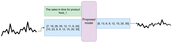
Figure 4.
Diagram of the synthetic data generation using an LLM (adapted from [28]).
4. Experiments
4.1. Evaluation
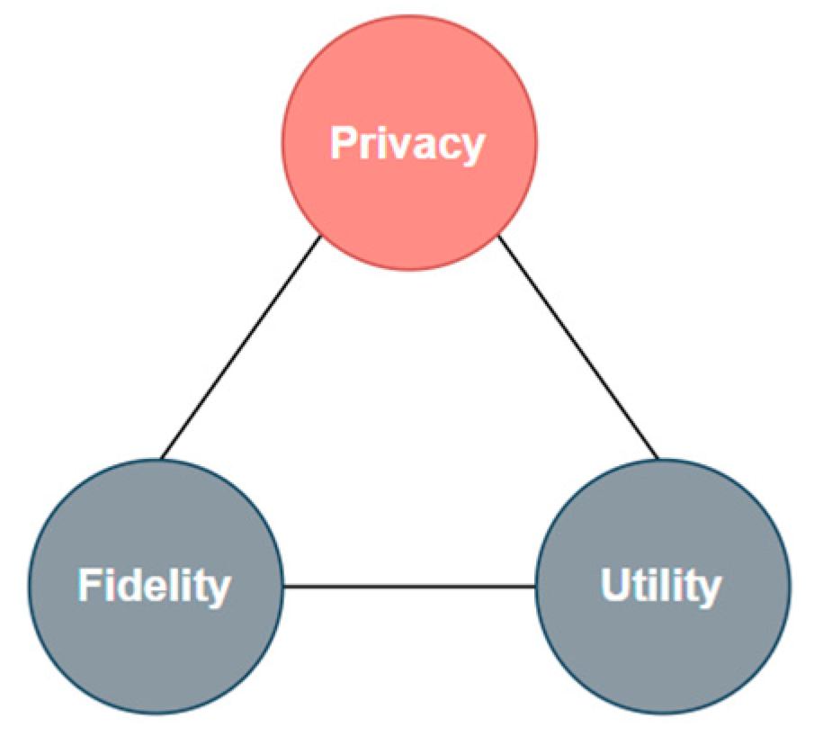
The goal of the proposed model is to generate synthetic data that are suitable for the tasks of data extension and reconstruction. Three dimensions are used to determine if the model outperforms existing SDGs [40]. Evaluating SD is not as simple as determining all the scores and selecting the one with the best values. SD cannot be optimized on all three dimensions simultaneously, which makes it necessary for a trade-off between fidelity, utility, and privacy to be made. The three dimensions are represented as a triangle in Figure 5.

Figure 5.
Synthetic data evaluation dimensions (adapted from [40]).
In the case of extension and reconstruction, fidelity and utility were chosen as the metrics to be optimized. Fidelity represents how similar the generated data are compared to the real data and is important in tasks where creating an accurate time series is important. The utility was then measured to determine how useful the generated data were for the problem. It is determined by using the generated data in prediction tasks using different algorithms. The last one was privacy. Storing and analyzing customer data or other important information is regulated and must respect the standards set. The generated SD should not leak information from the real dataset. Privacy cannot be optimized in the proposed model, and it is important to analyze it to determine how it performs against the other models. In this way, if there is not a significant difference, the model offers good enough performance on this metric.
Two datasets were used: online retail store data and financial data. The first dataset used to fine-tune the LLM model was M5 Forecasting—Accuracy [41]. It is a large-scale dataset created for the M5 Forecasting Competition hosted by the International Institute of Forecasters (IIF), which was released in 2020 and is designed to facilitate research and development in time series forecasting methods. It contains details about 42,840 hierarchical sales data from Walmart, making it suitable for evaluating the performance of forecasting models across diverse domains. The second dataset contains stock market data with historical daily prices of Nasdaq-traded stocks and ETFs [42]. The closing price was selected for the stocks and ETFs used in the experiments. The data were retrieved from Yahoo Finance.
4.2. Results
Multiple experiments were performed to compare the proposed model to the following models: GAN, TimeGAN, DoppelGANger, and LSTM. The system was tested on the three dimensions presented in Section 4.1. These determine how the model performs on the three dimensions and if it offers an improvement in fidelity and utility at the cost of privacy in the context of generating synthetic data for data extension and reconstruction.
The GAN model is the baseline model for generating synthetic datasets. It has the problems of lack of convergence, mode collapse, and vanishing gradient. TimeGAN improves it by preserving temporal dynamics, while DoppelGANger improves it further by using batch generation and auto-normalization, as well as an auxiliary discriminator to solve the initial problems of the GAN. The proposed model has enhanced temporal understanding, which makes it better for handling long-range temporal dependencies over the GAN-based models. It has a flexible contextualization compared with a fixed-length input on GANs and has better control over the data characteristics using fine-tuning. Some disadvantages of the proposed model include high computational complexity and the risk of overfitting. It can also function as a sequence learning problem after scaling and quantization of the time series input data. It can then be considered a forecasting model. The model was compared to an LSTM neural network.
4.2.1. Fidelity
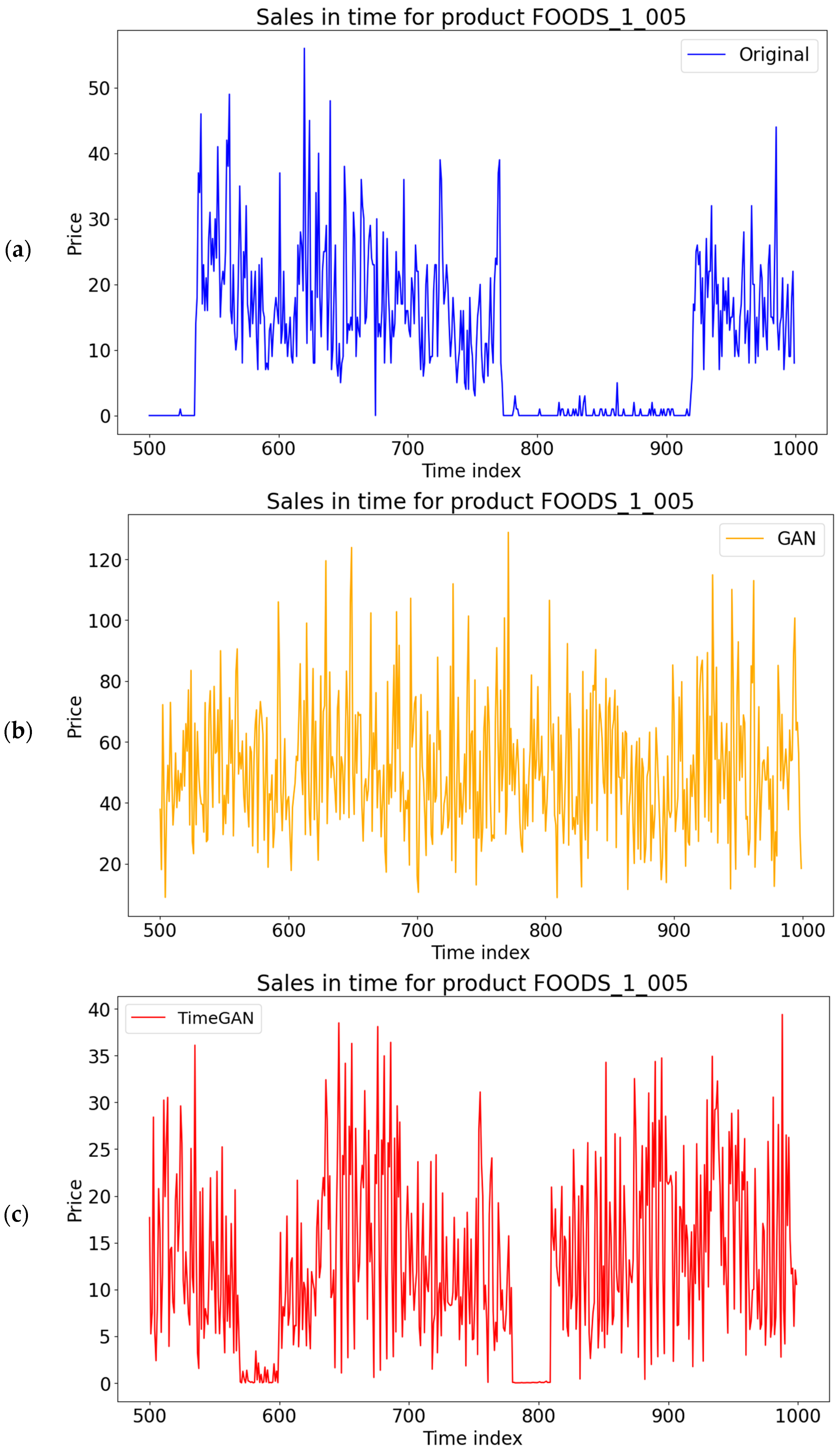
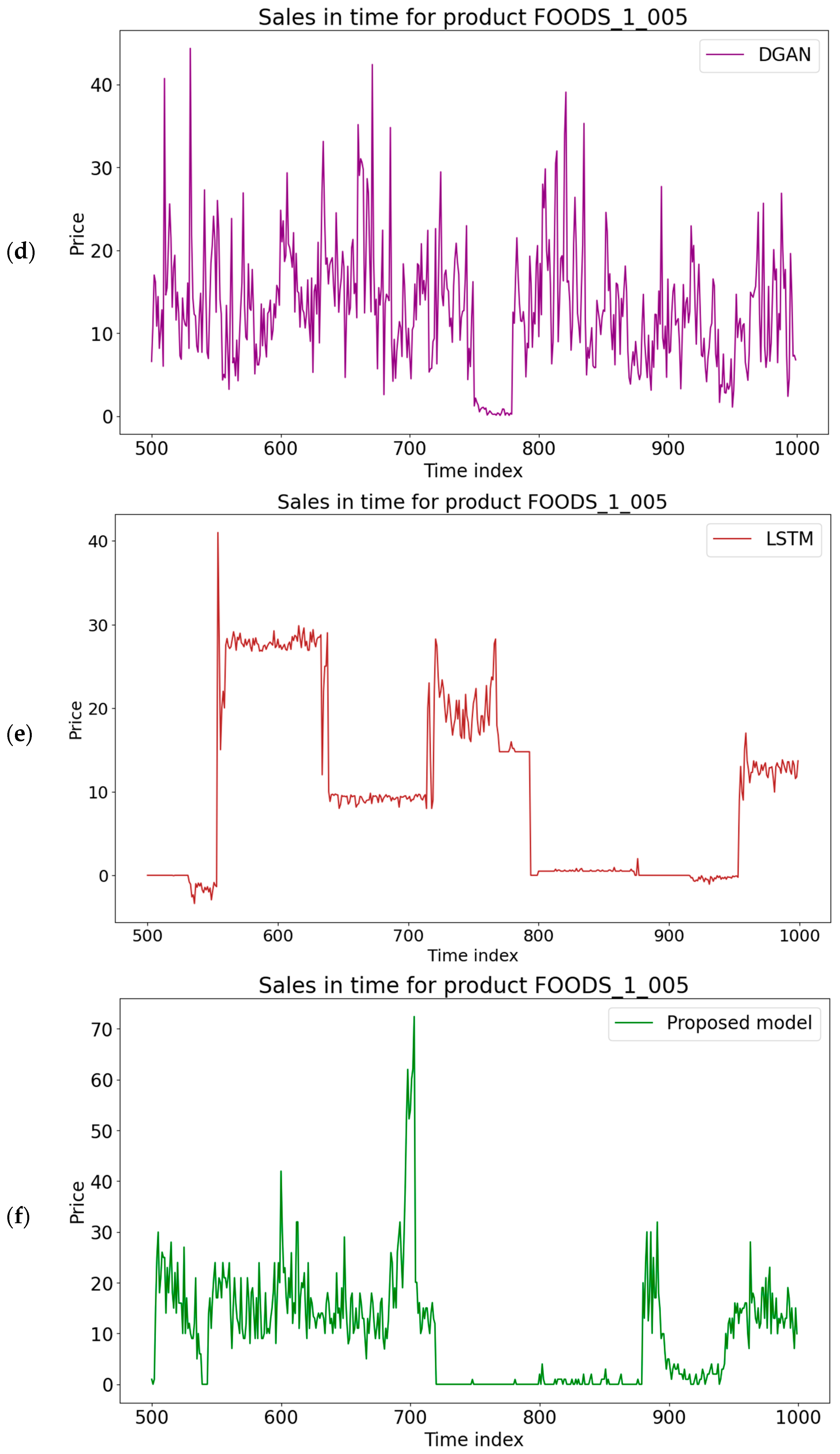
The original synthetic data were compared to the generated synthetic datasets both visually and using similarity metrics. Figure 6 contains the visualization of the time series on the M5 dataset. The proposed model has a higher similarity with the original dataset than the other models. While this is not ideal in every scenario for a general SDG, it has advantages in the cases of data extension and reconstruction. In extending the time series for the same products, it is important to maintain the trend in the time series and avoid being too general; otherwise, important information could be lost. This is important in business use cases for forecasting, where a similar trend is better than an average prediction, where the overall forecasting accuracy is higher.

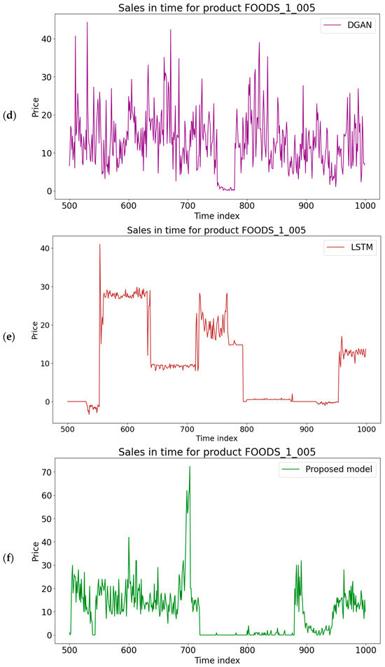
Figure 6.
The comparison of original and synthetically generated data for the analyzed methods: (a) original data; (b) GAN; (c) TimeGAN; (d) DGAN; (e) LSTM; (f) proposed model.
Data reconstruction has similar requirements, as it needs to hide the exact values while keeping a similar trend to be useful in those applications. Generated synthetic data are considered safer to use than original data, which have no protection and can leak important information. More details about the performance of the data are shown in the following metrics. The LLM generates the time series similar to the input time series, while the other models create results based on the training dataset provided. The graphs show promising results for the goal.
Comparisons of the non-temporal correlations between the four products selected from the M5 dataset are represented in Table 1, Table 2, Table 3, Table 4, Table 5 and Table 6 for the original data, the compared models, and the proposed model. Equation (3) shows the formula of and how it is calculated, where , are the individual sample points of variables , , and , are their respective means. The objective is to have similar correlations between variables of the synthetic data compared with the other models. The correlations between variables are similar and remain consistent across all the models.

Table 1.
Correlation in real data between products for the M5 dataset.
Table 2.
Correlation in synthetic data between products for the GAN on the M5 dataset.
Table 3.
Correlation in synthetic data between products for the TimeGAN on the M5 dataset.
Table 4.
Correlation in synthetic data between products for the DGAN on the M5 dataset.
Table 5.
Correlation in synthetic data between products for the LSTM on the M5 dataset.
Table 6.
Correlation in synthetic data between products for the proposed model on the M5 dataset.
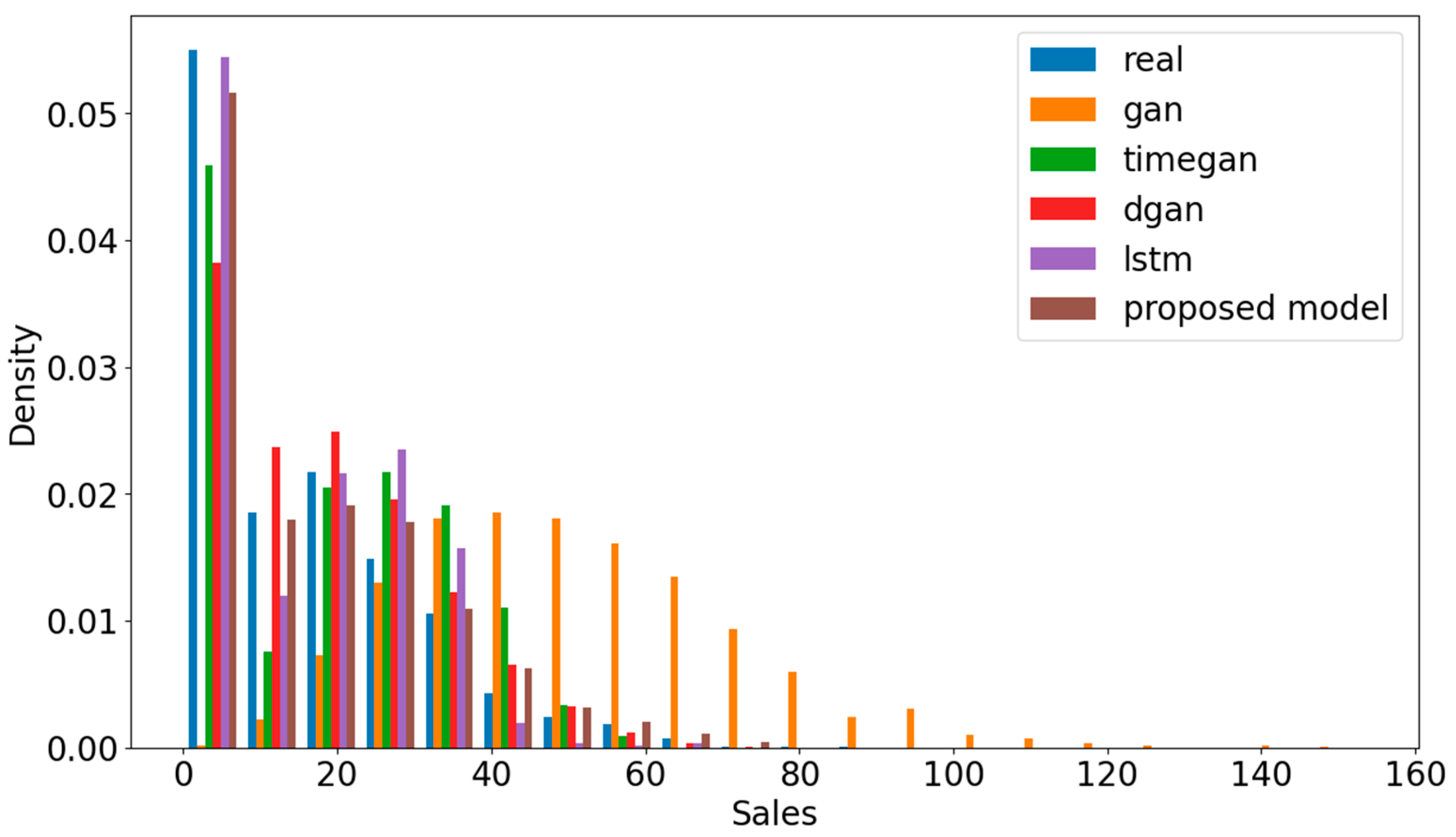
The distributions of output values for all the models are compared in Figure 7. The values should be close to the real dataset for a good synthetic dataset that follows the same patterns as the real data. The closer the values are to the real dataset, the more accurate the synthetic data are in terms of fidelity. Analyzing the density for the sales of each model, the proposed model shows results that are closest to the real values compared with the others.
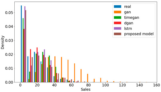
Figure 7.
Comparison of the distribution of output values for the selected models on the M5 dataset.
Other metrics to compare the similarity of the datasets are cosine similarity (CS) and Jensen–Shannon distance (JS) [43]. The JS distance is the square root of the JS divergence. The average values of those metrics are shown in Table 7 for the proposed model and the compared models. The results are given for both retail and financial datasets. The higher the value, the more similar the time series are on CS, and the opposite is true for JS. The expression for CS is presented in Equation (4), where , are the individual sample points of variables , . The JS distance is the square root of JS divergence and is shown in Equation (5), where is the pointwise mean of and , and D is the Kullback–Leibler divergence. The proposed model shows an improvement in similarity with the original data for CS and JS in both datasets.
Table 7.
Average cosine similarity and average Jensen–Shannon distance for the selected models.
Table 7.
Average cosine similarity and average Jensen–Shannon distance for the selected models.
| Model | Avg. Cosine Similarity (M5 Dataset) | Avg. JS Distance (M5 Dataset) | Avg. Cosine Similarity (Stocks Dataset) | Avg. JS Distance (Stocks Dataset) |
|---|---|---|---|---|
| GAN | 0.9124 | 0.3127 | 0.9158 | 0.3095 |
| TimeGAN | 0.8976 | 0.3271 | 0.9467 | 0.2803 |
| DoppelGANger | 0.9140 | 0.3116 | 0.9474 | 0.2799 |
| LSTM | 0.9197 | 0.9435 | ||
| Proposed model | 0.9208 | 0.2242 | 0.9484 | 0.2789 |
The discriminative score is another important metric in the evaluation of synthetic data to determine how well a model can distinguish between real and synthetic data samples. It evaluates the classification accuracy between original and synthetic data using a post hoc RNN network. The output is shown in Table 8, where the lower value is better. The proposed model has the lowest value, as confirmed in the visualization graphs. Compared with the LSTM, the results are better because the forecasting model aims to determine the most accurate future values, whereas a synthetic data generator must incorporate some randomization to avoid being too similar to the real data.
Table 8.
Discriminative score for the selected models.
Table 8.
Discriminative score for the selected models.
| Model | Discriminative Score (M5 Dataset) | Discriminative Score (Stocks Dataset) |
|---|---|---|
| GAN | 0.3923 | 0.4769 |
| TimeGAN | 0.1493 | 0.2177 |
| DoppelGANger | 0.1538 | 0.1692 |
| LSTM | 0.3475 | 0.06 |
| Proposed model | 0.1385 | 0.04 |
4.2.2. Utility
The predictive score [11] is used to evaluate the prediction performance on the train on synthetic tests in a real setting. A post hoc RNN architecture is used to predict one step ahead and report the performance in terms of MAE, as seen in Table 9. The forecasting score evaluates the performance using an XGBoost [44] model by forecasting five steps ahead in terms of MAE, which is shown in Table 9. The lower values offer a better utility for training machine learning models. The proposed model offers a better predictive score than TimeGAN in the M5 forecasting dataset and worse in the financial dataset due to the irregularities in stock market data. The forecasting score is better than TimeGAN in the M5 dataset and better than DoppelGANger in financial datasets. This shows the potential for the synthetic data to be useful in forecasting tasks.
Table 9.
Predictive and forecasting scores for the selected models.
Table 9.
Predictive and forecasting scores for the selected models.
| Model | Forecasting Score (M5 Dataset) | Predictive Score (M5 Dataset) | Forecasting Score (Stocks Dataset) | Predictive Score (Stocks Dataset) |
|---|---|---|---|---|
| Real data | 5.0202 | - | 14.8507 | - |
| GAN | 14.7066 | 0.2513 | 53.1305 | 0.2499 |
| TimeGAN | 3.7573 | 0.1867 | 17.2828 | 0.0389 |
| DoppelGANger | 4.7288 | 0.2310 | 5.7457 | 0.0494 |
| LSTM | 3.7828 | 0.2229 | 14.4989 | 0.2051 |
| Proposed model | 3.6635 | 0.1828 | 2.9812 | 0.2051 |
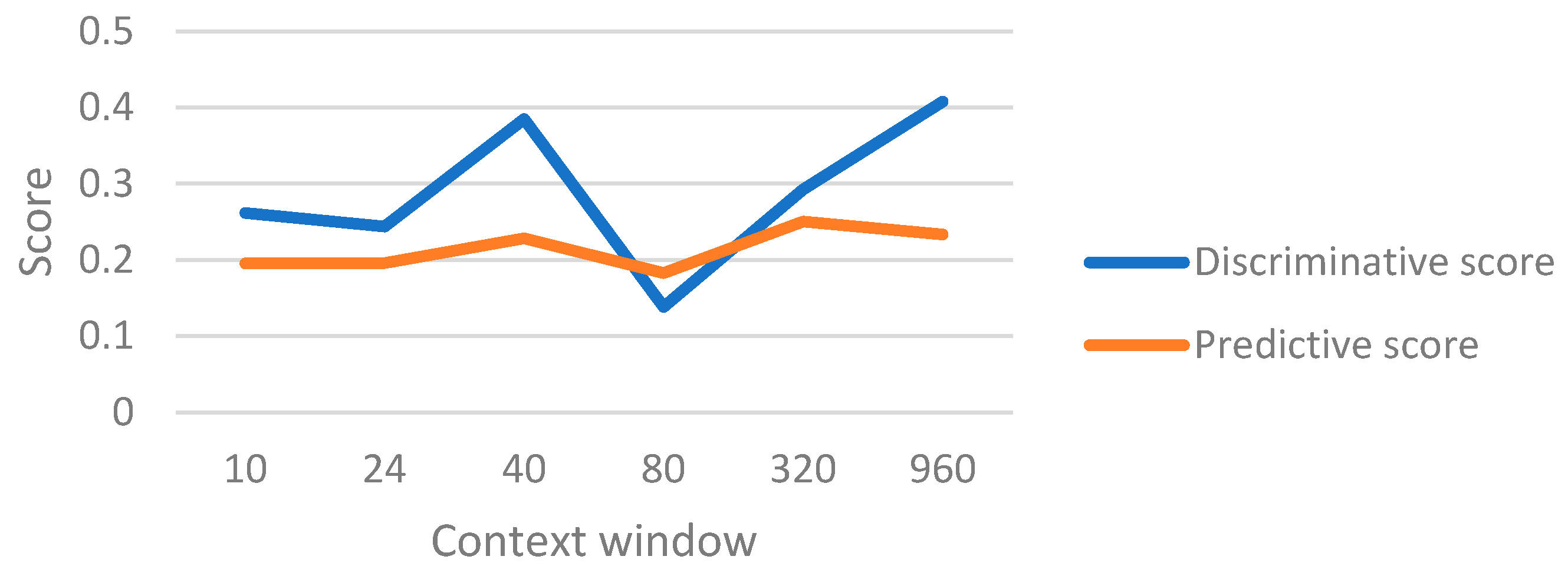
An experiment was conducted to determine the best value for the context window in the model. The discriminative and predictive scores by changing the context window size are shown in Figure 8 for the proposed model. It shows how the variation of the context size affects the results. The best value selected for context size was 80.
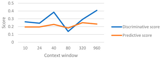
Figure 8.
Discriminative and predictive scores for the proposed model with different context sizes.
4.2.3. Privacy
While the model was not optimized for privacy, some experiments were performed to assess privacy against inference, which represents a set of metrics that determine the likelihood that an attacker will be able to reveal sensitive or private information from the synthetic dataset. The methods such as multi-layer perceptron (NumericalMLP), logistic regression (NumericalLR), support vector regression (NumericalSVR), and radius nearest neighbors (NumericalRadNN) [45] were employed to differentiate between real and synthetic data. The NumericalMLP method uses the full synthetic dataset and a few columns of real data (key fields) as input. A multi-layer perceptron neural network was trained to determine the output of the other values of real data (sensitive fields). The final score was 1 minus the average prediction score of the neural network. The other methods work similarly but use different regression methods. The best score is 1, which means the real data are safe from the attack, and the worst is 0, where an attacker can retrieve sensitive data. The results in Table 10 and Table 11 with the selected models are used to determine the protection score of the proposed model on the two different datasets. The proposed model offers an improvement in protection on the NumericalMLP metric and a decrease in protection for the other three metrics. This is expected, as the primary elements for optimization are fidelity and utility. An improvement in privacy could be made only with a trade-off in fidelity and utility.
Table 10.
Privacy against inference metrics for the selected models on the M5 dataset.
Table 10.
Privacy against inference metrics for the selected models on the M5 dataset.
| Model | NumericalMLP | NumericalLR | NumericalSVR | NumericalRadNN |
|---|---|---|---|---|
| GAN | 0.9481 | 0.2797 | 0.2983 | 0.8089 |
| TimeGAN | 0.9884 | 0.2721 | 0.2464 | 0.8904 |
| DoppelGANger | 0.9872 | 0.2616 | 0.2488 | 0.8552 |
| LSTM | 0.9884 | 0.2149 | 0.2180 | 0.8311 |
| Proposed model | 0.9931 | 0.2151 | 0.2181 | 0.8699 |
Table 11.
Privacy against inference metrics for the selected models on the stock market dataset.
Table 11.
Privacy against inference metrics for the selected models on the stock market dataset.
| Model | NumericalMLP | NumericalLR | NumericalSVR | NumericalRadNN |
|---|---|---|---|---|
| GAN | 0.5180 | 0.5530 | 0.6072 | 0.9695 |
| TimeGAN | 0.7677 | 0.0527 | 0.2491 | 0.9131 |
| DoppelGANger | 0.6120 | 0.0582 | 0.2570 | 0.9102 |
| LSTM | 0.5736 | 0.0513 | 0.1414 | 0.8811 |
| Proposed model | 0.5239 | 0.0507 | 0.1416 | 0.9090 |
4.3. Discussion
The experiments conducted with the proposed synthetic data generator highlight the increase in performance in optimizing the fidelity and utility metrics and demonstrate its effectiveness in creating synthetic data that are close to real data. The model has slightly worse results on privacy metrics, which is an expected trade-off. The results are consistent across the two datasets with online retail and financial data. Future improvements to the model could be made by using real-world data in different domains. Collecting the required data from businesses is a long-term process, and optimizations need to be made to perform better in different use cases.
The proposed model can be further employed to create a complete decision intelligence system. It can be extended to output not only the synthetic data but also the insights extracted from that data that are related to the decision that needs to be made. A scenario generator tool can be created, where the business executives can analyze how changing an input variable affects the output. An example can be a retail store that has multiple suppliers for the same products and should make a decision about what supplier to choose depending on how the market changes. If the decision maker changes the supplier, the model should predict the future revenue of the company based on past data. This result helps businesses to make data-driven decisions in an easy-to-understand format. Another domain for this application can be financial data, where a company can predict the stock price depending on the new markets that it enters.
However, there are some challenges of deploying in LLM into production. The first is managing the computational resources and costs required for (near) real-time inference. Data privacy needs to be ensured when handling sensitive information. Monitoring the model performance is essential in ensuring accurate results and improving the model as market conditions change and unexpected events can happen.
5. Conclusions
Synthetic data have an important role in business data analysis, where datasets for training machine learning models are not available or pose privacy concerns. The work conducted in this paper focused on solving the problems of data availability and data privacy for decision intelligence tools, which are useful for business executives to make data-driven decisions.
While GAN and VAE models were used to generate synthetic data with good performance, the current research focused on the transformer architecture. TimeGAN proposes a method that maintains the relationship between variables over time and improves the results of a GAN. DoppelGANger improves it further by using batch generation and auto-normalization to solve the initial problems of GANs. The model can also be seen as a sequence learning problem and is compared to an LSTM network, which has worse results. The evaluation of synthetic data is not standardized and needs to be optimized depending on the objective, making each model suitable for a certain task.
A model for generating synthetic data based on LLMs is proposed. It has and enhanced temporal understanding to handle long-range temporal dependencies, a flexible contextualization and uses fine-tuning to have a better control over the data characteristics. High computational complexity and risk of overfitting are some of its limitations.
The first step in creating the model is choosing the pre-trained LLM, which has general knowledge learned from a large amount of multi-source data as input. The second one is fine-tuning using a specialized dataset; it employs QLoRA to reduce the complexity of fine-tuning. An important task in using LLMs for generating time series data is determining how the data are converted for use as input to the LLM. There are multiple tokenization methods used for converting the raw numbers into simple tokens. The model uses mean scaling and quantization to achieve a better tokenization of numbers. The last step is the inference, which outputs the synthetic data in the correct format to be used for training different ML models.
Multiple experiments were performed in terms of fidelity, utility and privacy to determine synthetic data performance. The model was compared to GAN, TimeGAN, DoppelGANger, and LSTM models. Datasets with online retail and financial data were used. Regarding fidelity, the model showed an improvement in similarity based on data visualization, cosine similarity, Jensen–Shannon distance, and discriminative score. The utility also improved using the predictive score, which determines the performance of data in ML prediction tasks. The privacy was reduced, which was determined by using multiple machine learning models trained to determine the original data based on the synthetic data and some known columns of the original data. These include multi-layer perceptrons, logistic regression, support vector regression, and radius nearest neighbors. All experiments show that optimizing fidelity and utility has a trade-off of lower privacy, which is expected. The model demonstrates its effectiveness in creating synthetic data for the tasks of data extension and reconstruction.
Author Contributions
Conceptualization, A.G.; investigation, A.G.; methodology, A.G. and F.L.; software, A.G.; validation, A.G. and F.L.; writing—original draft, A.G. and F.L.; writing—review and editing, A.G. and F.L. All authors have read and agreed to the published version of the manuscript.
Funding
This research received no external funding.
Data Availability Statement
The datasets mentioned in the paper are publicly available at https://github.com/grigoras-alexandru/synthetic-data-llm (accessed on 11 July 2024).
Conflicts of Interest
The authors declare no conflict of interest.
References
- Pratt, L.Y.; Malcolm, N.E. The Decision Intelligence Handbook; O’Reilly Media, Inc.: Sebastopol, CA, USA, 2023. [Google Scholar]
- Creating Synthetic Time Series Data for Global Financial Institutions—A POC Deep Dive. Available online: https://gretel.ai/blog/creating-synthetic-time-series-data-for-global-financial-institutions-a-poc-deep-dive (accessed on 10 March 2024).
- Emam, K.E.; Mosquera, L.; Hoptroff, R. Practical Synthetic Data Generation—Balancing Privacy and the Broad Availability of Data; O’Reilly Media, Inc.: Sebastopol, CA, USA, 2020. [Google Scholar]
- Exploring Synthetic Data: Advantages and Use Cases. Available online: https://mailchimp.com/resources/what-is-synthetic-data/ (accessed on 10 March 2024).
- Goodfellow, I.J.; Pouget-Abadie, J.; Mirza, M.; Xu, B.; Warde-Farley, D.; Ozair, S.; Courville, A.; Bengio, Y. Generative Adversarial Nets. Adv. Neural Inf. Process. Syst. 2014, 27, 2672–2680. [Google Scholar]
- Kingma, D.P.; Welling, M. Auto-encoding Variational Bayes. Clin. Orthop. Relat. Res. arXiv 2013, arXiv:1312.6114. [Google Scholar]
- Vaswani, A.; Shazeer, N.; Parmar, N.; Uszkoreit, J.; Jones, L.; Gomez, A.N.; Kaiser, Ł.; Polosukhin, I. Attention Is All You Need. Adv. Neural Inf. Process. Syst. 2017, 30, 6000–6010. [Google Scholar]
- Hernandez, M.; Epelde, G.; Alberdi, A.; Cilla, R.; Rankin, D. Synthetic Data Generation for Tabular Health Records: A Systematic Review. Neurocomputing 2022, 493, 28–45. [Google Scholar] [CrossRef]
- Lu, Y.; Shen, M.; Wang, H.; Wang, X.; van Rechem, C.; Wei, W. Machine Learning for Synthetic Data Generation: A Review. arXiv 2023, arXiv:2302.04062. [Google Scholar]
- Choi, E.; Biswal, S.; Malin, B.; Duke, J.; Stewart, W.F.; Sun, J. Generating Multi-label Discrete Patient Records using Generative Adversarial Networks. In Proceedings of the 2nd Machine Learning for Healthcare Conference, PMLR, Boston, MA, USA; 2017; Volume 68, pp. 286–305. [Google Scholar]
- Yoon, J.; Jarrett, D.; van der Schaar, M. Time-Series Generative Adversarial Networks. Adv. Neural Inf. Process. Syst. 2019, 32, 5508–5518. [Google Scholar]
- Hui, J. GAN—Why It Is So Hard to Train Generative Adversarial Networks. Available online: https://jonathan-hui.medium.com/gan-why-it-is-so-hard-to-train-generative-advisory-networks-819a86b3750b (accessed on 10 March 2024).
- Lin, Z.; Jain, A.; Wang, C.; Fanti, G.; Sekar, V. Using GANs for Sharing Networked Time Series Data: Challenges, Initial Promise, and Open Questions. In Proceedings of the ACM Internet Measurement Conference ’20, Virtual, 27–29 October 2020; pp. 464–483. [Google Scholar]
- Solatorio, A.; Dupriez, O. REaLTabFormer: Generating Realistic Relational and Tabular Data using Transformers. arXiv 2023, arXiv:2302.02041. [Google Scholar]
- Borisov, V.; Seßler, K.; Leemann, T.; Pawelczyk, M.; Kasneci, G. Language Models are Realistic Tabular Data Generators. In Proceedings of the The Eleventh International Conference on Learning Representations, Virtual, 25–29 April 2022. [Google Scholar]
- Hameed, R.; Ahmadi, S.; Daneshfar, F. Transfer Learning for Low-Resource Sentiment Analysis. ACM Trans. Asian Low-Resour. Lang. Inf. Process. 2023, 37, 4. [Google Scholar]
- Daneshfar, F. Enhancing Low-Resource Sentiment Analysis: A Transfer Learning Approach. Passer 2024, 6, 265–274. [Google Scholar] [CrossRef]
- Kuchaiev, O.; Li, J.; Nguyen, H.; Hrinchuk, O.; Leary, R.; Ginsburg, B.; Kriman, S.; Beliaev, S.; Lavrukhin, V.; Cook, J.; et al. NeMo: A Toolkit for Building AI Applications Using Neural Modules. arXiv 2019, arXiv:1909.09577. [Google Scholar]
- Padhi, I.; Schiff, Y.; Melnyk, I.; Rigotti, M.; Mroueh, Y.; Dognin, P.; Ross, J.; Nair, R.; Altman, E. Tabular Transformers for Modeling Multivariate Time Series. In Proceedings of the International Conference on Acoustics, Speech and Signal Processing 2021, Toronto, ON, Canada, 6–11 June 2021; pp. 3565–3569. [Google Scholar]
- Zha, L.; Zhou, J.; Li, L.; Wang, R.; Huang, Q.; Yang, S.; Yuan, J.; Su, C.; Li, X.; Su, A.; et al. TableGPT: Towards Unifying Tables, Nature Language and Commands into One GPT. arXiv 2023, arXiv:2307.08674. [Google Scholar]
- Carballo, K.V.; Na, L.; Ma, Y.; Boussioux, L.; Zeng, C.; Soenksen, L.R.; Bertsimas, D. TabText: A Flexible and Contextual Approach to Tabular Data Representation. arXiv 2022, arXiv:2206.10381. [Google Scholar]
- Li, X.; Vangelis, M.; Huangyingrui, W.; Hee Hiong Ngu, A. TTS-GAN: A Transformer-Based Time-Series Generative Adversarial Network. In Proceedings of the International Conference on Artificial Intelligence in Medicine, Halifax, NS, Canada, 14–17 June 2022; pp. 133–143. [Google Scholar]
- Srinivasan, P.; Knottenbelt, W.J. Time-Series Transformer Generative Adversarial Networks. arXiv 2022, arXiv:2205.11164. [Google Scholar]
- Pang, C.; Jiang, X.; Pavinkurve, N.P.; Kalluri, K.S.; Minto, E.L.; Patterson, J.; Zhang, L.; Hripcsak, G.; Gürsoy, G.; Elhadad, N.; et al. CEHR-GPT: Generating Electronic Health Records with Chronological Patient Timelines. arXiv 2024, arXiv:2402.04400. [Google Scholar]
- Spathis, D.; Kawsar, F. The First Step is The Hardest: Pitfalls of Representing and Tokenizing Temporal Data for Large Language Models. J. Am. Med. Inform. Assoc. arXiv 2023, arXiv:2309.06236. [Google Scholar] [CrossRef] [PubMed]
- Jin, M.; Zhang, Y.; Chen, W.; Zhang, K.; Liang, Y.; Yang, B.; Wang, J.; Pan, S.; Wen, Q. Position: What Can Large Language Models Tell Us about Time Series Analysis. arXiv 2024, arXiv:2402.02713. [Google Scholar]
- Jin, M.; Wang, S.; Ma, L.; Chu, Z.; Zhang, J.Y.; Shi, X.; Chen, P.-Y.; Liang, Y.; Li, Y.-F.; Pan, S.; et al. Time-LLM: Time Series Forecasting by Reprogramming Large Language Models. arXiv 2023, arXiv:2310.01728. [Google Scholar]
- Sun, C.; Li, Y.; Li, H.; Hong, S. TEST: Text Prototype Aligned Embedding to Activate LLM’s Ability for Time Series. arXiv 2023, arXiv:2308.08241. [Google Scholar]
- Gruver, N.; Finzi, M.; Qiu, S.; Wilson, A.G. Large Language Models Are Zero-Shot Time Series Forecasters. arXiv 2024, arXiv:2310.07820. [Google Scholar]
- Junkai, L.; Weizhi, M.; Yang, L. Modeling Time Series as Text Sequence A Frequency-Vectorization Transformer for Time Series Forecasting. 2024. Available online: https://openreview.net/forum?id=N1cjy5iznY (accessed on 18 March 2024).
- Xu, K.; Chen, L.; Patenaude, J.M.; Wang, S. RHINE: A Regime-Switching Model with Nonlinear Representation for Discovering and Forecasting Regimes in Financial Markets. In Proceedings of the Proceedings of the 2024 SIAM International Conference on Data Mining (SDM), Houston, TX, USA, 18–20 April 2024; pp. 526–534. [Google Scholar]
- Qian, Z.; Cebere, B.C.; van der Schaar, M. Synthcity: Facilitating Innovative Use Cases of Synthetic Data in Different Data Modalities. arXiv 2023, arXiv:2301.07573. [Google Scholar]
- Manousakas, D.; Aydorem, S. On the Usefulness of Synthetic Tabular Data Generation. In Proceedings of the International Conference on Machine Learning, Honolulu, HI, USA, 23–29 July 2023. [Google Scholar]
- Raffel, C.; Shazeer, N.; Roberts, A.; Lee, K.; Narang, S.; Matena, M.; Zhou, Y.; Li, W.; Liu, P.J. Exploring the Limits of Transfer Learning with a Unified Text-to-Text Transformer. arXiv 2023, arXiv:1910.10683. [Google Scholar]
- Kudo, T.; Richardson, J. SentencePiece: A Simple and Language Independent Subword Tokenizer and Detokenizer for Neural Text Processing. In Proceedings of the 2018 Conference on Empirical Methods in Natural Language Processing: System Demonstrations, Brussels, Belgium, 2–4 November 2018; pp. 66–71. [Google Scholar]
- Dettmers, T.; Pagnoni, A.; Holtzman, A.; Zettlemoyer, L. Qlora: Efficient Finetuning of Quantized LLMs. arXiv 2024, arXiv:2305.14314. [Google Scholar]
- Ansari, A.F.; Stella, L.; Turkmen, C.; Zhang, X.; Mercado, P.; Shen, H.; Shchur, O.; Rangapuram, S.S.; Arango, S.P.; Kapoor, S.; et al. Chronos: Learning the Language of Time Series. arXiv 2024, arXiv:2403.07815. [Google Scholar]
- Salinas, D.; Flunkert, V.; Gasthaus, J.; Januschowski, T. DeepAR: Probabilistic Forecasting with Autoregressive Recurrent Networks. Int. J. Forecast. 2020, 36, 1181–1191. [Google Scholar] [CrossRef]
- Rabanser, S.; Januschowski, T.; Flunkert, V.; Salinas, D.; Gasthaus, J. The Effectiveness of Discretization in Forecasting: An Empirical Study on Neural Time Series Models. In Proceedings of the MileTS ’20: 6th KDD Workshop on Mining and Learning from Time Series, San Diego, CA, USA, 24 August 2020. [Google Scholar]
- Haddad, F. How to Evaluate the Quality of the Synthetic Data—Measuring from the Perspective of Fidelity, Utility, and Privacy. 2022. Available online: https://aws.amazon.com/blogs/machine-learning/how-to-evaluate-the-quality-of-the-synthetic-data-measuring-from-the-perspective-of-fidelity-utility-and-privacy/ (accessed on 10 March 2024).
- Howard, A.; Makridakis, S. M5 Forecasting—Accuracy. Available online: https://kaggle.com/competitions/m5-forecasting-accuracy (accessed on 10 March 2024).
- Onyshchak, O. Stock Market Dataset. Available online: https://www.kaggle.com/datasets/jacksoncrow/stock-market-dataset (accessed on 25 July 2024).
- Nielsen, F. On the Jensen-Shannon Symmetrization of Distances Relying on Abstract Means. Entropy 2019, 21, 485. [Google Scholar] [CrossRef]
- Chen, T.; Guestrin, C. Xgboost: A scalable tree boosting system. In Proceedings of the 22nd ACM SIGKDD International Conference on Knowledge Discovery and Data Mining, San Francisco, CA, USA, 13–17 August 2016; pp. 785–794. [Google Scholar]
- Patki, N.; Wedge, R.; Veeramachaneni, K. The Synthetic data vault. In Proceedings of the IEEE International Conference on Data Science and Advanced Analytics (DSAA), Montreal, QC, Canada, 17–19 October 2016; pp. 399–410. [Google Scholar]
Disclaimer/Publisher’s Note: The statements, opinions and data contained in all publications are solely those of the individual author(s) and contributor(s) and not of MDPI and/or the editor(s). MDPI and/or the editor(s) disclaim responsibility for any injury to people or property resulting from any ideas, methods, instructions or products referred to in the content. |
© 2024 by the authors. Licensee MDPI, Basel, Switzerland. This article is an open access article distributed under the terms and conditions of the Creative Commons Attribution (CC BY) license (https://creativecommons.org/licenses/by/4.0/).