Abstract
Tracking control of the output probability density function presents significant challenges, particularly when dealing with unknown system models and multiplicative noise disturbances. To address these challenges, this paper introduces a novel tracking control algorithm based on reinforce-ment Q-learning. Initially, a B-spline model is employed to represent the original system, thereby transforming the control problem into a state weight tracking issue within the B-spline stochastic system model. Moreover, to tackle the challenge of unknown stochastic system dynamics and the presence of multiplicative noise, a model-free reinforcement Q-learning algorithm is employed to solve the control problem. Finally, the proposed algorithm’s effectiveness is validated through comprehensive simulation examples.
Keywords:
tracking control; probability density function; reinforcement learing; B-spline model; Q-learning; model-free MSC:
93E35
1. Introduction
The surge in interest in stochastic control stems from its applicability to diverse real-world systems, including aerospace, chemical, textile, and maritime machinery [1,2]. Gaussian processes in control can be managed through mean and variance manipulation [3], but non-Gaussian processes, such as particle scale distribution in paper processing [4], flame shape dynamics [5], and chemical polymerization molecular weight distribution [6], necessitate a more comprehensive approach. Wang’s 1996 innovation introduced probability density function (PDF) control [7,8,9], utilizing B-spline functions to bypass the Gaussian assumption limitations [10]. This has led to a range of stochastic control frameworks in both theoretical and practical realms, particularly in target tracking, where systems often aim to track distributions rather than values [11]. In detail, this method applies a B-spline model to represent the system’s dynamic probability density function (PDF) by mapping the weights of the B-spline function to a dynamic state–space model. This approach shifts the focus from controlling the shape of the PDF to aligning the weights with predefined values. Under this framework, numerous significant papers have been published. For example, Luan’s output PDF control tackles static tracking [12]. However, the controller design in most of the papers within this framework heavily relies on precise knowledge of the PDF model. Specifically, it requires the state–space model, derived from the PDF via the B-spline network, to be accurate for effective controller design. Meeting this requirement is challenging in many real-world industrial systems, limiting the practical application and development of this framework.
Multiplicative noise, which poses significant challenges due to its signal-dependent nature and non-linear characteristics, appears in various applications. However, a great number of studies, including those utilizing the algorithms proposed under Wang’s framework, do not account for the influence of multiplicative noise in their system modeling. Although Yang’s fully probabilistic design under Wang’s framework addresses this issue by incorporating multiplicative noise into the model [13], it necessitates precise knowledge of the system’s model parameters. Consequently, there is still a gap between this method and practical real-world applications.
Another important aspect often neglected in this framework is the consideration of time-varying targets. In many industrial contexts, time-varying targets are essential and present additional challenges for controller design. However, most studies within this framework tend to overlook this factor, which further complicates the practical application and effectiveness of the framework in real-world scenarios [9].
To address these barriers, this paper employs Wang’s B-spline framework to develop a model-free control approach that enables dynamic weights to adapt to a time-varying target pattern. In our design, we utilize Q-learning-based Linear Quadratic Tracking Control (LQT) as a controller to achieve the tracking goal. Traditional LQT often struggle with the complexities of real-world systems, highlighting the necessity for model-free control strategies. Thus, reinforcement learning, particularly strategy iteration, is employed here to handle control and scheduling tasks without requiring complete model information [14]. As a model-free technique, reinforcement learning optimizes control by learning under given constraints [11,15]. The concept of L-Extra-Sampled (Les)-dynamics was introduced in [16], providing a new perspective for addressing reinforcement learning problems in partially observable linear Gaussian systems. However, the research in this paper primarily focuses on linear Gaussian systems, which may limit the method’s applicability to non-Gaussian systems. In [17], an algorithm based on Q-learning was proposed to handle time-varying linear discrete-time systems with complete dynamic uncertainties. Although the algorithm is model-independent, it may require more computational resources to compute the Q-function and update the policy when dealing with high-dimensional systems. Ref. [18] introduced extreme value theory into reinforcement learning, proposing a new online and offline maximum entropy reinforcement learning update rule [19]. This rule avoids the difficulty of estimating the maximum Q-value in continuous action space. In [20], an efficient offline Q-learning method was proposed to solve the data-driven discrete-time linear quadratic regulator problem. This approach does not require knowledge of the system dynamic model and demonstrates advantages over existing methods in simulations. In [21], a Q-learning based iterative learning control (ILC) framework for fault estimation (FE) and fault-tolerant control (FTC) was proposed to address the actuator fault problem in multiple-input multiple-output (MIMO) systems. However, traditional reinforcement learning methods are inefficient, consuming significant time and requiring continuous adjustment. The efficiency of reinforcement learning can be enhanced by integrating it with optimal control techniques. For instance, in [22], the successful application of Q-learning to handle discrete systems with uncertain parameters was demonstrated, improving tracking control performance. Similarly, Xue’s extension to two-time-scale systems showed favorable outcomes [23]. However, these findings are based on deterministic models and neglect the system randomness and uncertainties. By solving the Riccati equation for quadratic optimal control of linear stochastic systems with unknown parameters, we improve learning efficiency and achieve model-free tracking control. This approach allows for effective control even in the presence of random disturbances, addressing the limitations of traditional methods and enhancing the practical applicability of our framework.
In summary, this paper utilizes Wang’s B-spline framework to develop a model-free control approach, enabling dynamic weights to adapt to a target time-varying pattern. In the case of an unknown stochastic system model, we can change the output PDF shape by controlling the weights. This approach expands the scope of application for stochastic systems in output PDF control. Output PDF control is employed to monitor and manage the distribution of key parameters during the production process, which helps enhance product quality and decrease scrap rates. For instance, in the semiconductor manufacturing industry, controlling the distribution of parameters such as etching depth and doping concentration during wafer fabrication ensures consistent chip performance. Similarly, in the automobile manufacturing industry, controlling the distribution of coating thickness during the painting process improves surface quality and anti-corrosion performance. By leveraging the B-spline basis functions and the model-free reinforcement Q-learning algorithm, we can effectively handle unknown system dynamics and multiplicative noise, achieving precise control over the output PDF shape. This method facilitates accurate PDF shape tracking and establishes a theoretical foundation for PDF monitoring in non-Gaussian stochastic systems, making it highly applicable to real-world industrial contexts. The contributions of this paper can be summarized as follows:
- 1
- By integrating the reinforcement learning method with the LQR control algorithm, the control framework proposed in this paper effectively addresses the challenge of PDF tracking control in stochastic systems with unknown parameters, eliminating the need for precise knowledge of the system’s model parameters.
- 2
- By utilizing B-spline functions to approximate the PDF, our method converts the PDF tracking problem into a state tracking problem with dynamic weights.
- 3
- The multiplicative noise is being considered while modeling the PDF under the B-spline framework, reflecting a more accurate representation of complex and realistic uncertainties.
- 4
- The consideration of time-varying PDF target, which are crucial in many real-world applications but often overlooked in previous studies, enhances the practical applicability of the framework.
- 5
- The framework combines optimal control principles with reinforcement learning, specifically Q-learning, to significantly enhance the performance and accelerate the learning speed of RL algorithms.
The remainder of this paper is organized as follows: Section 2 provides a detailed description of the problem and the B-spline model of the PDF. In Section 3, the optimal control law is derived based on the performance metrics, and the implementation algorithm is presented. Section 4 demonstrates the application of the controller through two numerical examples. Finally, Section 5 summarizes the conclusions and outlines potential future work.
2. Problem Description
2.1. PDF Description Based on B-Spline
Modeling the output PDF of a controlled system by solving partial differential equations can be challenging when using first principles, complicating the development of an effective control strategy [24]. To overcome this, the B-spline approach can be employed to approximate the PDF curve by mapping weights to basis functions. B-spline basis functions are a flexible and widely used class of functions that can adapt to various interpolation and fitting requirements. They can be classified by order: first-order, second-order, third-order and fourth-order B-spline basis functions. Among these, third-order B-spline basis functions are the most commonly used for cubic polynomial functions because they strike a good balance between smoothness and computational complexity. Specifically, given a known interval , where the output PDF is continuous and bounded, the PDF can be expressed using n B-spline basis functions as follows:
where (with ) represents the weight and represents pre-selected n basis functions, which can include Gaussian, radial basis, or wavelet functions. Given that is a PDF defined on the interval , it is subject to the following mathematical constraints:
To satisfy Equation (2), only weights are independent, which allows us to express the distribution in the following form:
where denotes the weight set, represents the vector of basis functions, and is a scalar associated with the basis functions. Based on Equations (5) and (6), we can see that the choice of basis functions determines and . From Equation (1) to Equation (6), it is evident that the B-spline model enables the control of the output PDF shape by manipulating independent weight vectors [25].
2.2. PDF Tracking Control Problem
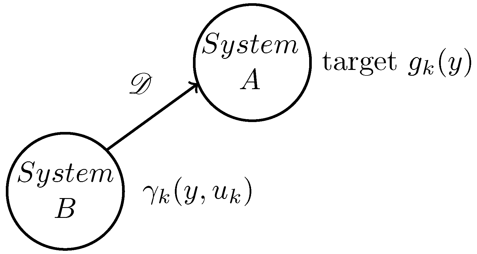
The tracking problem is a prevalent issue in the field of control, including in stochastic control systems. In conventional control fields, the objective often involves directing the system to follow a predefined value. Conversely, in stochastic control systems, the goal shifts to having the system track a predetermined probability density function (PDF). Figure 1 illustrates the tracking diagram where system B tracks system A. System A, despite its unknown structure, can monitor its output in real time, allowing access to the output PDF distribution at any given time k. On the other hand, system B is a controlled system with established dynamics and employs a control input u to produce its output . The objective is to align the output distribution of system B with that of system A, with quantifying the disparity between the two distributions. The details of the system and tracking control issues outlined above are further elaborated in the subsequent section.

Figure 1.
Diagram of the tracking system.
Consider the stochastic system with output PDF , whose dynamics is formed as follows:
where the distribution of the system output y is denoted by and represents the system input.
Based on the B-spline model (3), denoting as the weights corresponding to the basis functions, the output PDF of the tracking system B can be represented as:
The tracking target is a dynamic PDF with the following manner:
where in Equation (9) represent the pre-set target weights corresponding to each basis function.
Subsequently, the shaping of the output PDF over the interval can be achieved by controlling the weight state . Within the framework of the B-spline model outlined in [8], the dynamics of the weight states for the B-spline model-based PDF are described as follows:
where and are the corresponding weight system parameters and represents the state-based model randomness, whose distribution is given by:
where M is the variance of .
From Equations (7) to (10), we observe that the system’s PDF is dynamic, leading to the derivation of a state–space model for the weights to represent the PDF’s dynamics. However, obtaining precise model parameters, , , and , is challenging. Existing control strategies often rely on precise model parameters, necessitating that , , and in Equation (10) are known accurately. This assumption is difficult to meet in many real-world industrial processes.
To address this limitation, this study explores the application of data-driven methods, specifically reinforcement learning within machine learning, to mitigate the dependence on model parameters. Reinforcement learning, characterized by its objective to maximize reward through iterative optimization, offers a promising solution to the optimal control problem [26]. By employing Q-learning, one of a reinforcement learning algorithm, the need for explicit model knowledge is alleviated, as it enables the determination of optimal control strategies based solely on system operational data. This approach enables the controlled variable to effectively track the desired trajectory without requiring knowledge of the model parameters.
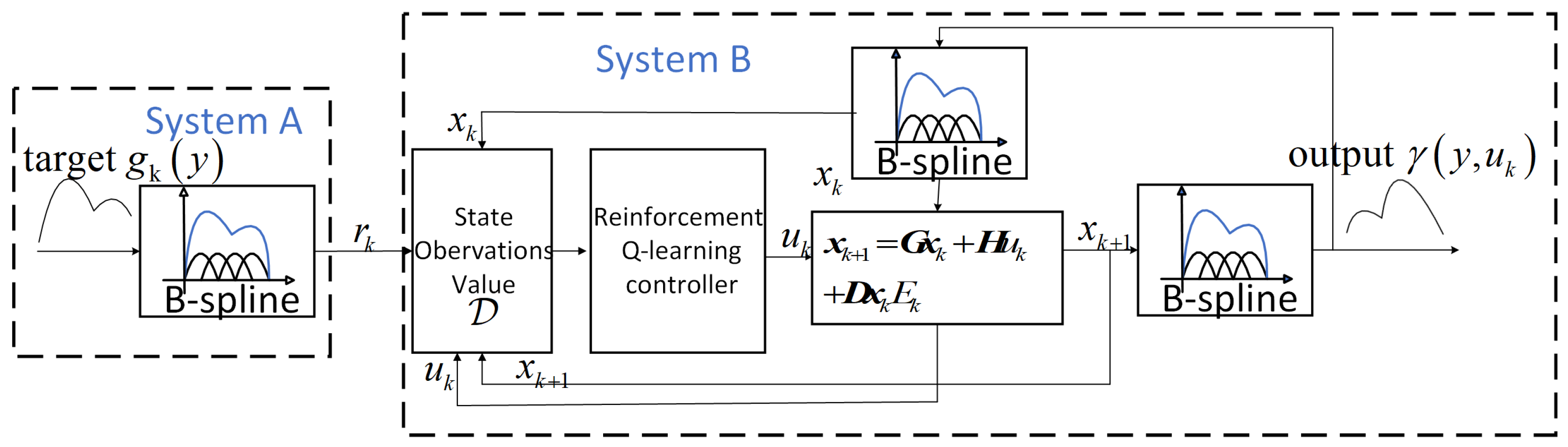
The control flowchart is depicted in Figure 2. After selecting the B-spline basis functions, the time-varying target weight in Figure 2 is determined based on the target distribution using the B-spline principle. The system input is derived by assessing both the target and system weights using a reinforcement Q-learning control, which will be detailed in the subsequent section. The weight is then updated through B-spline principle modeling and the input . The output distribution is obtained by correlating the weight with the basis function. It is important to note that the model error component is characterized by multiplicative noise, and represents the appropriately dimensioned weight matrix. The weights are iteratively updated according to the model to control the output distribution.
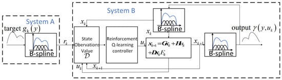
Figure 2.
System control structure diagram.
There are many methods to address multiplicative noise, and it is necessary to choose the appropriate method for different application scenarios to effectively reduce the noise’s impact. Techniques such as logarithmic transformation, adaptive filtering, wavelet transformation, statistical methods, and specially designed filters can significantly improve the quality and reliability of signal processing. However, within a reinforcement learning framework, multiplicative noise can be directly learned, thus eliminating the need for these additional processing methods.
Building on this framework, the control objective for such stochastic system is to design a state feedback controller that enables the weight to track the target weight . Consequently, the PDF shape tracking control problem is transformed into a weight tracking control problem. The details of the controller design will be presented in the next section.
3. Control Algorithm
In this section, we introduce the reinforcement Q-learning control algorithm to achieve the tracking objective of the weight state. The primary motivation for choosing reinforcement learning control is to attain optimal tracking control in the presence of unknown model parameters. Additionally, the reinforcement Q-learning method is employed to establish an optimal control iterative solution structure, which proves to be more efficient than traditional reinforcement learning algorithms. The specific details are elaborated below.
3.1. General Control Solution of LQT for Systems with Multiplicative Noise
In this section, we consider the infinite-horizon linear quadratic tracking problem with multiplicative noise. This developed algorithm will then be utilized as a foundation to create our model-free Q-learning control method.
Denoting the target weight for the LQT problem which are generated by the B-spline model based on the expected PDF output is , based on the system dynamics Equation (10), we construct the augmented system:
where the augmented state is given by:
For the regular infinite-horizon LQT problem, the objective is to design an optimal controller for the system in Equation (10), ensuring that the weight tracks a reference trajectory . This can be achieved by minimizing the following infinite-horizon performance index:
where denotes the mathematical expectation over the noise {E(0),E(1),…}, and and are symmetric matrices. The performance index in Equation (14) can be rewritten using Equation (13) as:
where with . The stochastic system (12) is said to be mean-square stabilizable if there exists a state feedback control [27]:
When the model parameters are known, there are multiple methods to determine the optimal feedback gains and the associated optimal cost. The optimal cost can be derived from the solution of the generalized algebraic Riccati Equation (GARE) [28]:
The optimal gain matrix is as follows:
As verified in [29], the standard conditions for the uniqueness and existence of a solution to the standard ARE require that is stabilizable and is detectable [30].
3.2. Data-Driven Reinforcement Learning for LQT Problems
In this section, we establish the action-value Q-function for reinforcement learning to iteratively solve the Riccati equation for quadratic optimal control of stochastic systems with unknown model parameters using data. The Q-function is equivalent to the cost function in optimal control, and we need to optimize this Q-function to achieve the optimal value through the control strategy [31]. We construct our Q-function according to the standard control method. Firstly, we need to defined the Q-function. If the control policy, such as in Equation (16), is a mean-square stabilization control policy, then the Q-function should be defined in the desired form. Thus, the Q-function is defined as follows:
where is defined in Equation (15). The Bellman equation transforms an infinite sum of terms into a simpler, future-term form. Thus, based on the discrete-time LQT Bellman equation and Equation (19):
where P is defined in Equation (17). The Q-function can be further extended as follows:
where is the discount factor. This discount factor is crucial because it prevents the reward from increasing to infinity as the time step approaches infinity, thereby making the infinitely long control process evaluable. The discount factor represents the expectation of future rewards. A smaller discount factor places more emphasis on the reward in the current state, while a larger discount factor emphasizes future rewards. However, in the context of an infinite-time control process, the condition holds if and only if the reference trajectory is Schur stable. The selection of the discount factor depends on the desired effect, involving a balance between exploration and exploitation of the algorithm. By incorporating augmented system dynamics Equation (12), the Q-function becomes:
To simplify the computation of the Q-function, we introduce a kernel matrix , emphasizing its quadratic nature in the variables:
The optimal control action can then be derived by setting the gradient of Q-Function with respect to to zero, leading to a policy formula based on the Riccati-type solution. Applying the condition to Equation (23), we can obtain:
Define the extended state as:
The Q-function can then be written as the following form by substituting Equation (30) into Equation (20):
where
The multiplicative noise is then incorporated into the kernel matrix to participate in the policy iteration without requiring additional consideration.
The algorithm is structured around two main components:
- 1
- Policy Evaluation:Estimating the Q-function based on current policy and updating the kernel matrix using collected data by Equation (33).
- 2
- Policy Improvement:Adjusting the control policy to minimize future Q-function values thereby optimizes system performance over time. Policy iteration can be implemented using least squares (LS) with the data tuple [22].
Through these steps, the reinforcement Q-learning algorithm iteratively refines its estimates and policy, adapting to changes in system dynamics and performance criteria without requiring prior knowledge of the underlying system model. The multiplicative noise is embedded within the kernel matrix using the data-driven method. This approach not only enhances the flexibility of the control system, but also improves its robustness in handling real-world operational variabilities.
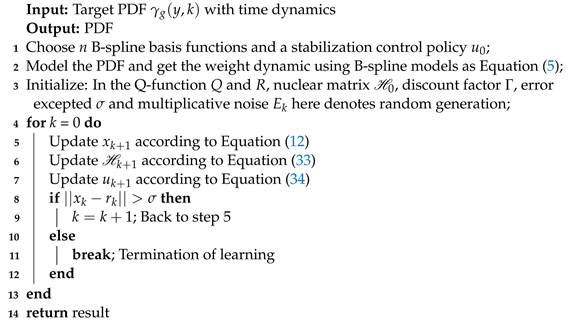
Algorithm 1 provides a structured approach to implement the proposed control framework, ensuring that each step is clearly defined and actionable.
| Algorithm 1: Tracking control framework with output probability density function |
 |
4. Simulation Result
In this section, we demonstrate the effectiveness of the model-free PDF tracking control algorithm through two numerical simulations. During the simulation process, the algorithm does not have any knowledge of the system model and relies solely on numerical calculations.
We start by choosing the B-spline basis functions, which are crucial for transforming the original system into a form suitable for our control algorithm. B-spline basis functions are flexible and can be tailored to various interpolation and fitting requirements. Specifically, we use third-order B-spline basis functions because they provide a good balance between smoothness and computational complexity. The B-spline basis functions selected are as follows:
where
As per constraint (2), only the corresponding weights for three of the four B-spline basis functions are necessary.
- Example 1
The fourth weight is linearly dependent on the first three weights, thereby reducing the model order to three. For example, 1, we use the same model as in reference [32] for comparison to demonstrate the difference between model-based and model-free approaches. By comparing the results, we can highlight the advantages and limitations of the proposed model-free reinforcement Q-learning algorithm against traditional model-based methods. Thus, the coefficient matrix of the system model is given by:
with , , .
In the described model, represents the state weight matrix, is the control matrix, is the random weight matrix of the noise term, and is the Gaussian noise. Note that the parameters , , and are assumed unknown. The target weights change every 100 steps, alternating between and . Additionally, the initial state of the system is set at . The noise covariance follows the distribution given by . The performance index, as indicated in Equation (14), employs and , with a discount factor . The parameter is chosen to be a suitably small value . The initial kernal matrix is given by:
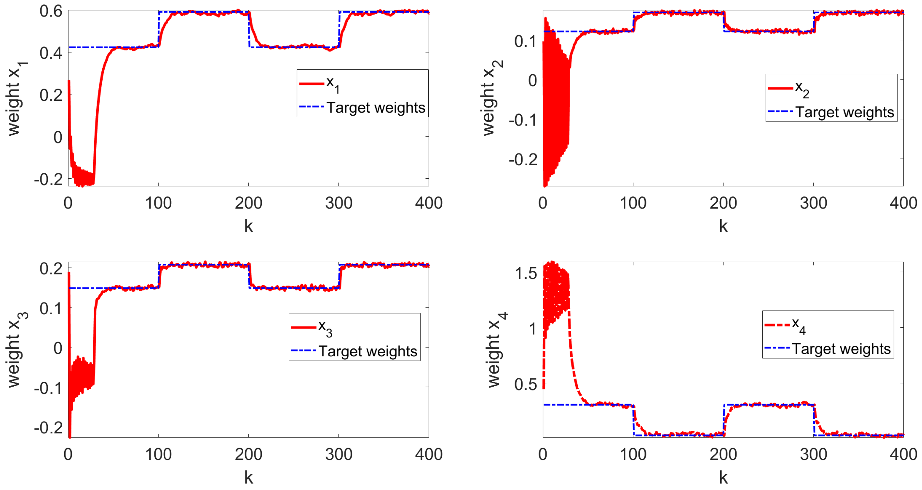
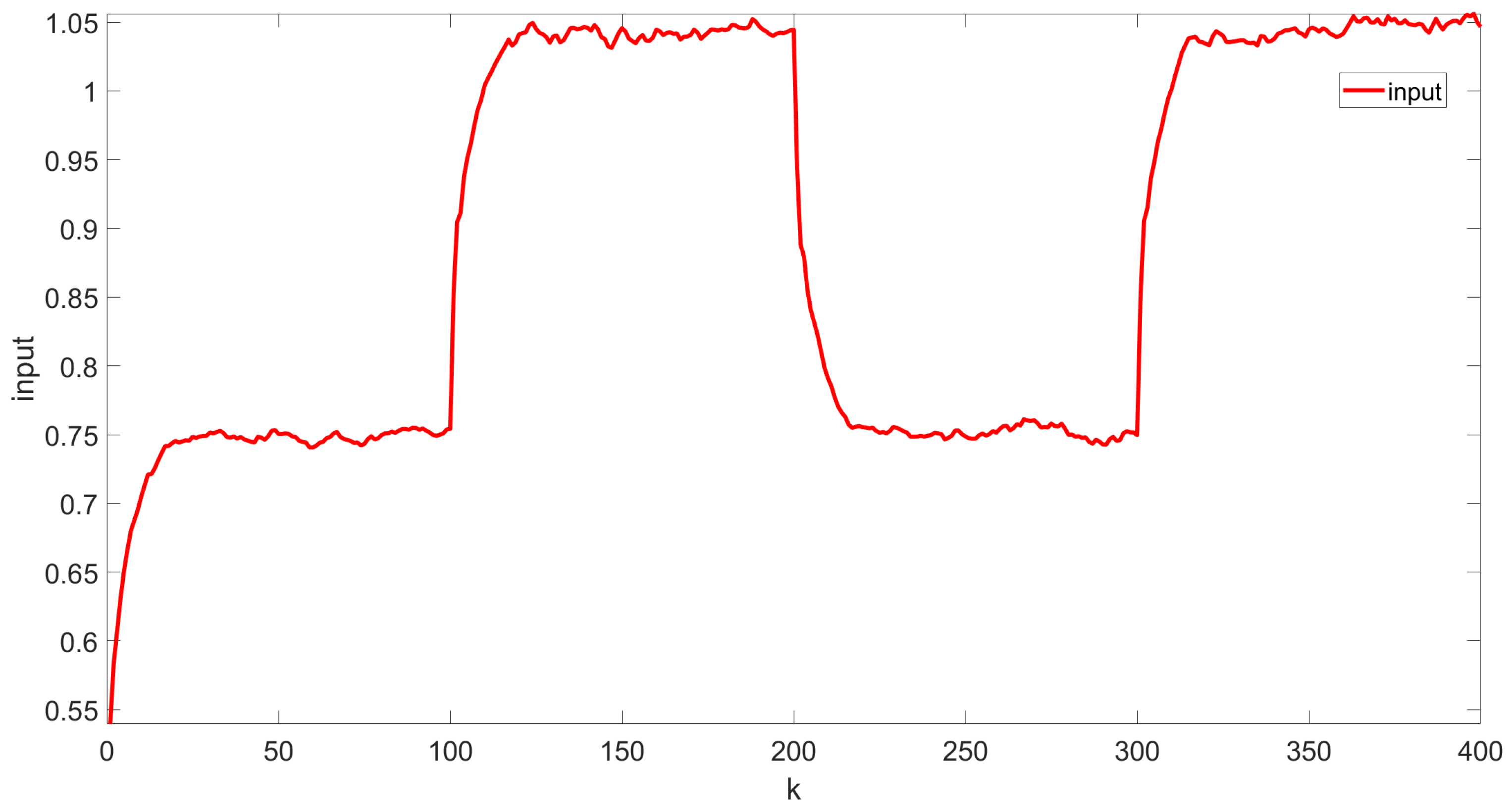
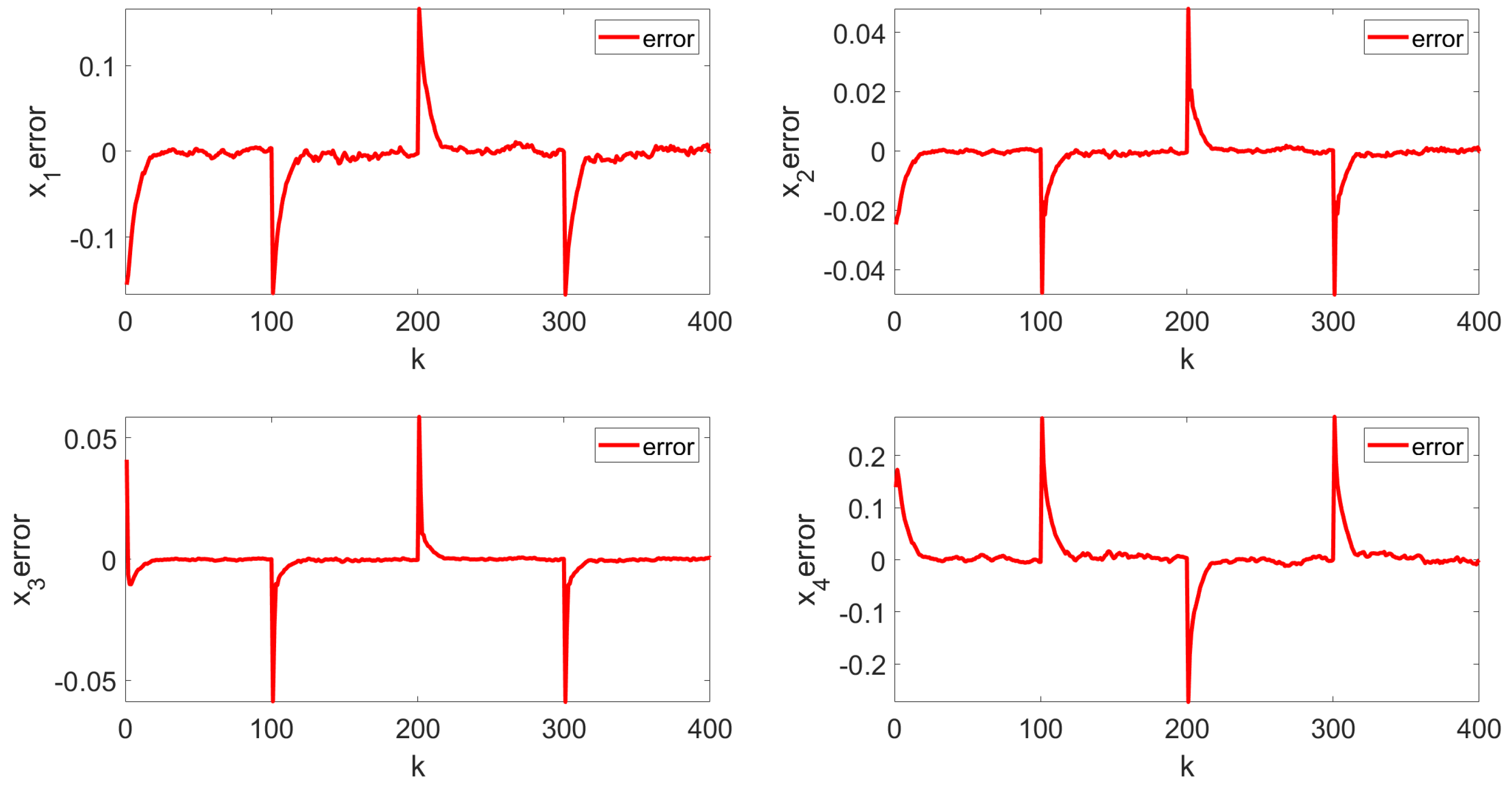
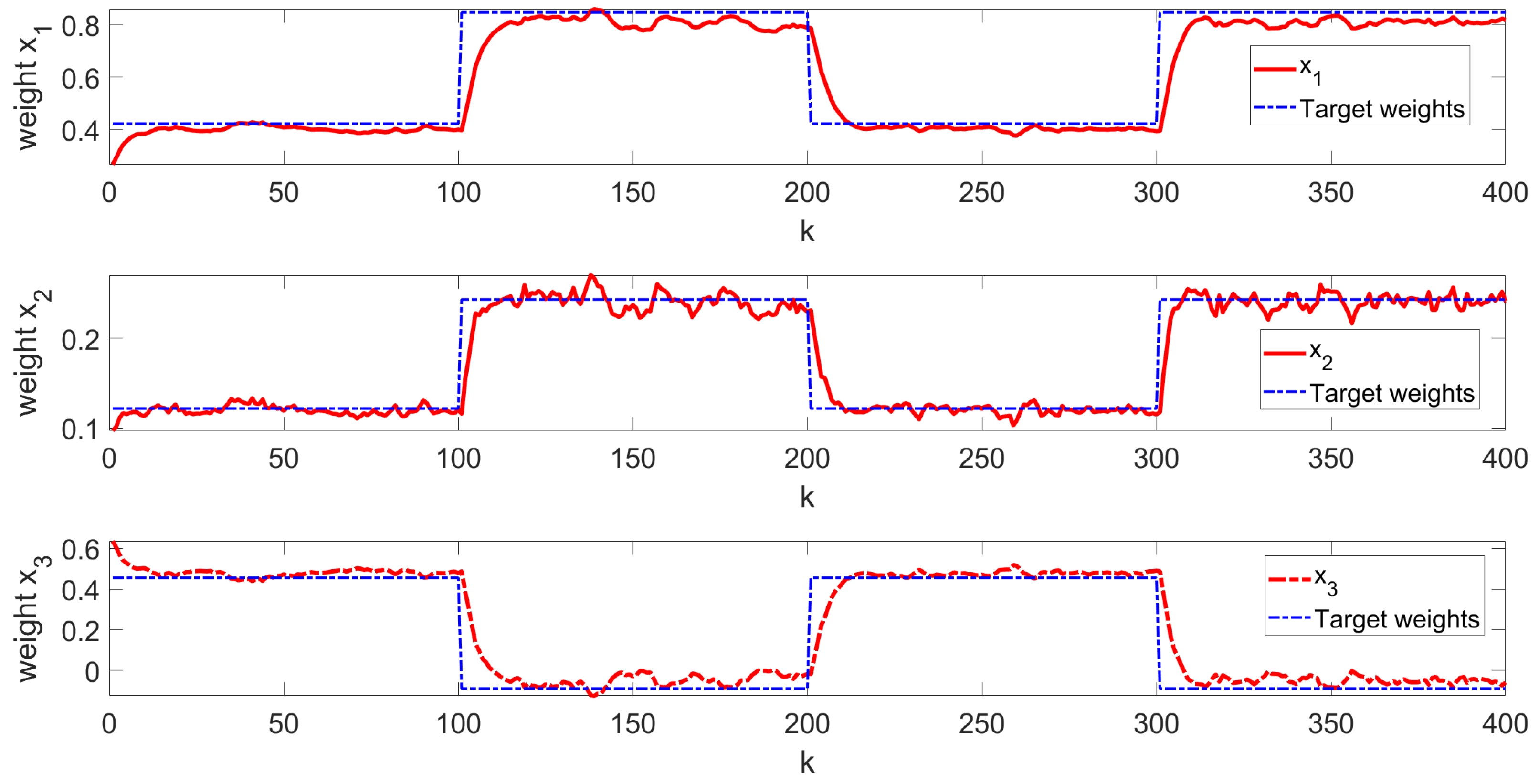
The simulation results are shown in Figure 3, Figure 4, Figure 5, Figure 6 and Figure 7. Figure 3 illustrates the weight tracking effect during the online learning process. It is evident that the algorithm begins with exploration and converges around the 40th iteration, demonstrating its computational efficiency. Notably, in Figure 4, the red line represents the weight tracking curve under the enhanced Q-learning algorithm, while the blue dashed line represents the target reference curve. The weights , , and are controlled states, whereas , which is linearly related to the other weights and excluded from control due to constraints, is also shown. Figure 4 further shows the control of the four weights and their corresponding target reference curves after the learning is completed. This demonstrates that the reinforcement Q-learning algorithm successfully tracks the specified target weights after learning. Figure 5 presents the system control input, with the red line indicating the control input curve under the reinforcement Q-learning algorithm. This curve aligns synchronically with the target configuration change and is smooth enough for practical use. Figure 6 illustrates the output curve of the reinforcement Q-learning algorithm, which consistently follows the desired PDF shape at each time instant. It also presents the results of the target weights integrated with the PDF output derived from the B-spline model. For example, in controlling the flame shape, this curve represents the flame shape at each moment. Despite the unknown system parameters, the output curve achieves the desired PDF shape, highlighting the effective utilization of the data. Figure 7 shows the tracking error curve of the four states. It can be seen from the figure that, despite the presence of multiplicative noise interference, the tracking effect remains very good. The tracking error only experiences a jump when the tracking weight changes, and in the remaining cases, it is essentially near 0. Finally, the mean square error of the tracking is calculated to be very small, specifically 0.0285, indicating that the tracking effect is good. These results indicate that the proposed control framework effectively enables the system’s PDF to track a predefined PDF shape without requiring specific knowledge of the system parameters.
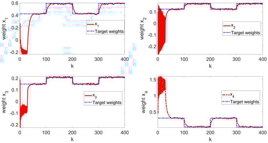
Figure 3.
Online learning process state curve.
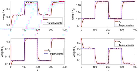
Figure 4.
Learning ending state curve.
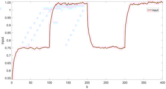
Figure 5.
Control input curve.
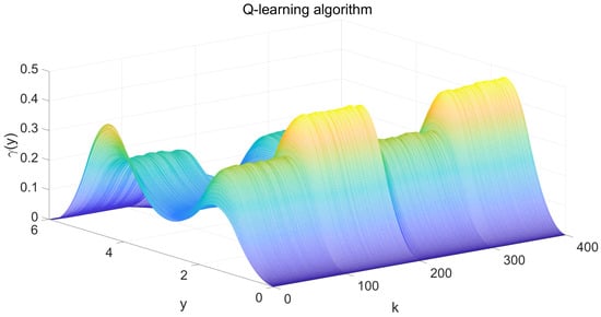
Figure 6.
System output PDF of 3D drawings.
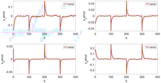
Figure 7.
Tracking error.
- Example 2
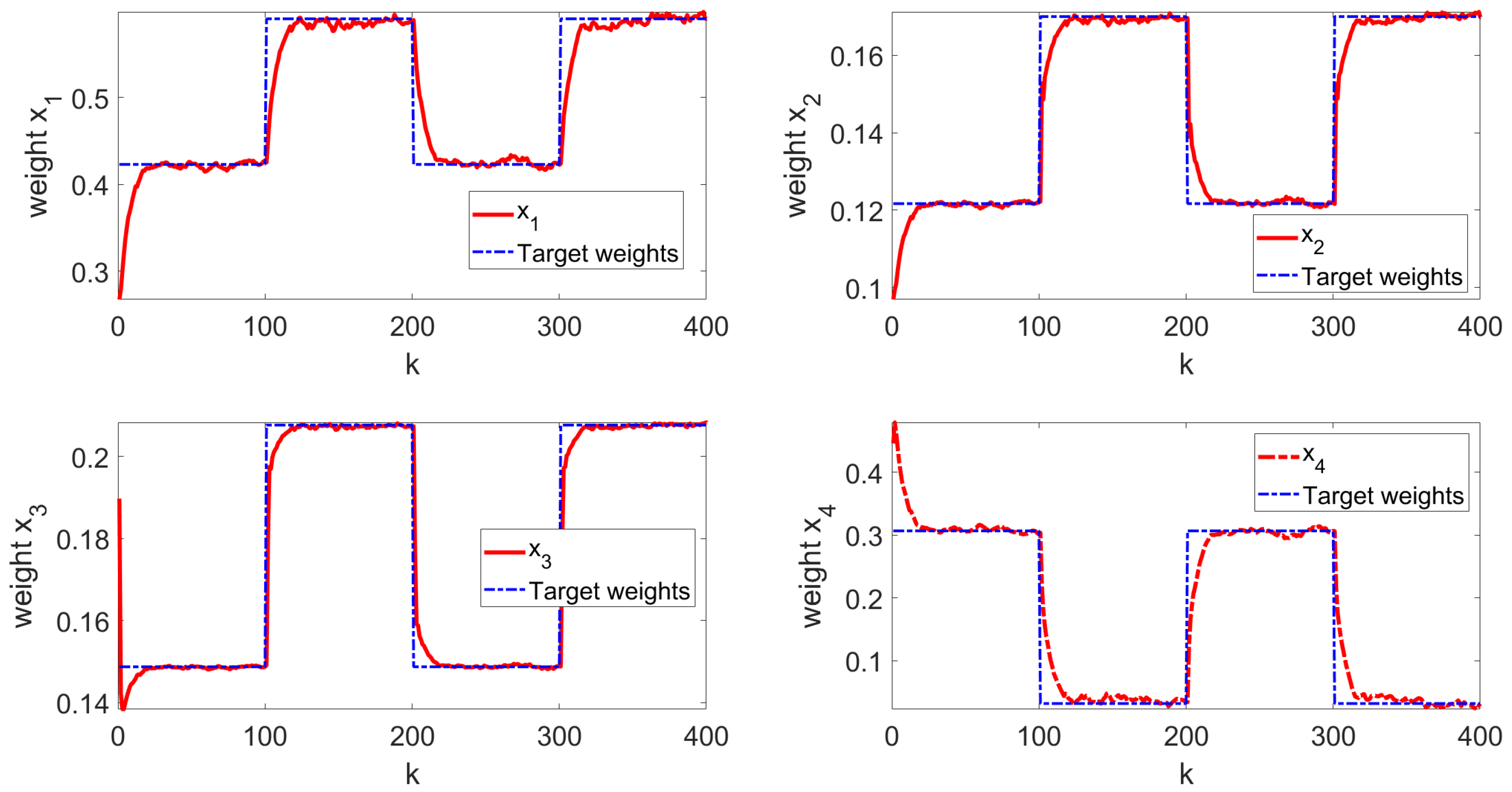
To strengthen the argument for the algorithm’s applicability in model-free scenarios, we provide another numerical simulation example, with , , . The target weights change every 100 steps, alternating between and . Additionally, the initial state of the system is set at . The noise covariance follows the distribution given by . The initial kernal matrix is
The simulation results are illustrated in Figure 8. In this figure, the red solid line represents the system state under our control, while the blue dashed line indicates the target weight. As shown, the system states successfully tracks the pre-set time-varying references. Additionally, the mean square error is calculated to be 0.1561, demonstrating the effective control performance. This result clearly shows that even without a model, the second-order stochastic system can accurately track the target weight.
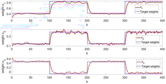
Figure 8.
Learning ending state curve.
Through two numerical simulation examples, we observe that the overall tracking error is minimal, the response speed is rapid, and the learning efficiency is high in both systems. This indicates that our control method is effective across different systems. Additionally, the mapping relationship between the systems is established using B-spline function fitting, which allows for controlling the PDF shape by tracking the target weight. Furthermore, the presented approach does not require prior knowledge of the model, enabling flexible back-and-forth switching control of the PDF shape.
5. Conclusions
This paper addresses the challenge of output distribution shape tracking in stochastic distribution systems by developing a learning-based, model-free control algorithm within the B-spline model framework to approximate the PDF. This method simplifies the complex issue of PDF shaping into a more manageable problem of dynamic weight modification, treating the system’s inherent randomness and inaccuracies as state-dependent noises, which closely mirror real-world complexities. To handle time-varying targets and reduce dependency on precise model knowledge, an extended Reinforcement Q-learning algorithm is applied in this framework. Simulation results confirm the method’s effectiveness, demonstrating its ability to accurately track varying distribution shapes. Using the data-driven method to control, it greatly removes the limitation that most control methods need system model parameters. Additionally, this approach eliminates the need to address complexities arising from multiplicative noise issues.
Author Contributions
Conceptualisation, Y.Z. (Yong Zhang); Methodology, Y.Z. (Yuyang Zhou); Validation, W.Y.; Writing—original draft preparation, W.Y.; Resources, Y.Z. (Yong Zhang); Writing—review and editing, Y.Z. (Yuyang Zhou); funding acquisition, Y.R. All authors have read and agreed to the published version of the manuscript.
Funding
This work was supported in part by the National Natural Science Foundation of China under Grant 62263026, Grant 62063027, the Fundamental Research Funds for Inner Mongolia University of Science and Technology under Grant 2024QNJS003, the Inner Mongolia Natural Science Foundation under Grant 2023MS06001, the Program for Young Talents of Science and Technology in Universities of Inner Mongolia Autonomous Region under Grant NJYT22057, the Fundamental Research Funds for Inner Mongolia University of Science and Technology under Grant 2023RCTD028, and the Inner Mongolia Autonomous Region Control Science and Engineering Quality Improvement and Cultivation Discipline Construction Project.
Institutional Review Board Statement
Not applicable.
Informed Consent Statement
Not applicable.
Data Availability Statement
Data are contained within the article.
Conflicts of Interest
The authors declare no conflicts of interest.
References
- Ren, M.; Zhang, Q.; Zhang, J. An introductory survey of probability density function control. Syst. Sci. Control Eng. 2019, 7, 158–170. [Google Scholar] [CrossRef]
- Lu, J.; Han, L.; Wei, Q.; Wang, X.; Dai, X.; Wang, F.Y. Event-triggered deep reinforcement learning using parallel control: A case study in autonomous driving. IEEE Trans. Intell. Veh. 2023, 8, 2821–2831. [Google Scholar] [CrossRef]
- Filip, I.; Dragan, F.; Szeidert, I.; Albu, A. Minimum-variance control system with variable control penalty factor. Appl. Sci. 2020, 10, 2274. [Google Scholar] [CrossRef]
- Li, M.; Zhou, P. Predictive PDF control of output fiber length stochastic distribution in refining process. Acta Autom. Sin. 2019, 45, 1923–1932. [Google Scholar]
- Sun, X.; Xun, L.; Wang, H.; Dong, H. Iterative learning control of singular stochastic distribution model of jet flame temperature field. J. Beijing Univ. Technol. 2013, 33, 523–528. [Google Scholar]
- Cao, L.; Wu, H. MWD modeling and control for polymerization via B-spline neural network. J. Chem. Ind. Eng. China 2004, 55, 742–746. [Google Scholar]
- Wang, H.; Yue, H. Output PDF control of stochastic distribution systems: Modelling control and applications. Control Eng. China 2003, 10, 193–197. [Google Scholar]
- Wang, H.; Zhang, J. Bounded stochastic distributions control for pseudo-ARMAX stochastic systems. IEEE Trans. Autom. Control. 2001, 46, 486–490. [Google Scholar] [CrossRef]
- Zhang, Q.; Zhou, Y. Recent advances in non-Gaussian stochastic systems control theory and its applications. Int. J. Netw. Dyn. Intell. 2022, 1, 111–119. [Google Scholar] [CrossRef]
- Wang, H. Bounded Dynamic Stochastic Systems: Modelling and Control, 1st ed.; Springer Science & Business Media: London, UK, 2000; pp. 15–34. [Google Scholar]
- Huang, E.; Cheng, Y.; Hu, W. Tracking control of multi-agent systems based on reset control. Control. Eng. China 2022, 29, 6. [Google Scholar]
- Luan, X.; Liu, F. Finite time stabilization of output probability density function of stochastic systems. Control Decis. 2009, 24, 1161–1166. [Google Scholar]
- Zhou, J.; Wang, H. Optimal tracking control of the output probability density functions: Square root B-spline model. Control Theory Appl. 2005, 22, 369–376. [Google Scholar]
- Hansen-Estruch, P.; Kostrikov, I.; Janner, M.; Kuba, J.G.; Levine, S. Idql: Implicit q-learning as an actor-critic method with diffusion policies. arXiv 2023, arXiv:2304.10573. [Google Scholar]
- Carmona, R.; Laurière, M.; Tan, Z. Model-free mean-field reinforcement learning: Mean-field MDP and mean-field Q-learning. Ann. Appl. Probab. 2023, 33, 5334–5381. [Google Scholar] [CrossRef]
- Yaghmaie, F.A.; Modares, H.; Gustafsson, F. Reinforcement Learning for Partially Observable Linear Gaussian Systems Using Batch Dynamics of Noisy Observations. IEEE Trans. Autom. Control. 2024. [Google Scholar] [CrossRef]
- Nguyen, H.; Dang, H.B.; Dao, P.N. On-policy and off-policy Q-learning strategies for spacecraft systems: An approach for time-varying discrete-time without controllability assumption of augmented system. Aerosp. Sci. Technol. 2024, 146, 108972. [Google Scholar] [CrossRef]
- Meyn, S. Stability of Q-learning through design and optimism. arXiv 2023, arXiv:2307.02632. [Google Scholar]
- Garg, D.; Hejna, J.; Geist, M.; Ermon, S. Extreme q-learning: Maxent rl without entropy. arXiv 2023, arXiv:2301.02328. [Google Scholar]
- Lopez, V.G.; Alsalti, M.; Müller, M.A. Efficient off-policy Q-learning for data-based discrete-time LQR problems. IEEE Trans. Autom. Control. 2023, 68, 2922–2933. [Google Scholar] [CrossRef]
- Wang, R.; Zhuang, Z.; Tao, H.; Paszke, W.; Stojanovic, V. Q-learning based fault estimation and fault tolerant iterative learning control for MIMO systems. ISA Trans. 2023, 142, 123–135. [Google Scholar] [CrossRef]
- Kiumarsi, B.; Lewis, F.L.; Modares, H.; Karimpour, A.; Naghibi-Sistani, M.B. Reinforcement Q-learning for optimal tracking control of linear discrete-time systems with unknown dynamics. Automatica 2014, 50, 1167–1175. [Google Scholar] [CrossRef]
- Xue, W.; Fan, J.; Lopez, V.G.; Jiang, Y.; Chai, T.; Lewis, F.L. Off-policy reinforcement learning for tracking in continuous-time systems on two time scales. IEEE Trans. Neural Netw. Learn. Syst. 2020, 32, 4334–4346. [Google Scholar] [CrossRef] [PubMed]
- Zha, W.; Li, D.; Shen, L.; Zhang, W.; Liu, x. Review of neural network-based methods for solving partial differential equations. Chin. J. Theor. Appl. Mech. 2022, 54, 543–556. [Google Scholar]
- Zhang, Y.; Zhou, P.; Lv, D.; Zhang, S.; Cui, G.; Wang, H. Inverse calculation of burden distribution matrix using B-spline model based PDF control in blast furnace burden charging process. IEEE Trans. Ind. Inform. 2023, 19, 317–327. [Google Scholar] [CrossRef]
- Hu, B.; Zhang, K.; Li, N.; Mesbahi, M.; Fazel, M.; Başar, T. Toward a theoretical foundation of policy optimization for learning control policies. Annu. Rev. Control. Robot. Auton. Syst. 2023, 6, 123–158. [Google Scholar] [CrossRef]
- Wang, D.; Wang, J.; Zhao, M.; Xin, P.; Qiao, J. Adaptive multi-step evaluation design with stability guarantee for discrete-time optimal learning control. IEEE/CAA J. Autom. Sin. 2023, 10, 1797–1809. [Google Scholar] [CrossRef]
- Gravell, B.; Esfahani, P.M.; Summers, T. Learning optimal controllers for linear systems with multiplicative noise via policy gradient. IEEE Trans. Autom. Control. 2020, 66, 5283–5298. [Google Scholar] [CrossRef]
- Willems, J.L.; Willems, J.C. Feedback stabilizability for stochastic systems with state and control dependent noise. Automatica 1976, 12, 277–283. [Google Scholar] [CrossRef]
- Lewis, F.L.; Vrabie, D.; Syrmos, V.L. Optimal Control; John Wiley & Sons: Hoboken, NJ, USA, 2012. [Google Scholar]
- Xiao, B.; Lam, H.K.; Su, X.; Wang, Z.; Lo, F.P.-W.; Chen, S.; Yeatman, E. Sampled-data control through model-free reinforcement learning with effective experience replay. J. Autom. Intell. 2023, 2, 20–30. [Google Scholar] [CrossRef]
- Yang, Y.; Zhang, Y.; Zhou, Y. Tracking Control for Output Probability Density Function of Stochastic Systems Using FPD Method. Entropy 2023, 25, 186. [Google Scholar] [CrossRef]

Disclaimer/Publisher’s Note: The statements, opinions and data contained in all publications are solely those of the individual author(s) and contributor(s) and not of MDPI and/or the editor(s). MDPI and/or the editor(s) disclaim responsibility for any injury to people or property resulting from any ideas, methods, instructions or products referred to in the content. |
© 2024 by the authors. Licensee MDPI, Basel, Switzerland. This article is an open access article distributed under the terms and conditions of the Creative Commons Attribution (CC BY) license (https://creativecommons.org/licenses/by/4.0/).