Article

Transverse Compression of a Thin Inhomogeneous Elastic Layer

by
Ahmed S. M. Alzaidi
1,
Julius Kaplunov
2,
Barbara Zupančič
3 and
Anatolij Nikonov
4,*
1
Department of Mathematics and Statistics, College of Science, Taif University, Taif 21944, Saudi Arabia
2
School of Computing and Mathematics, Keele University, Newcastle ST5 5BG, UK
3
Theory Department, National Institute of Chemistry, 1000 Ljubljana, Slovenia
4
Faculty of Mechanical Engineering, University of Ljubljana, 1000 Ljubljana, Slovenia
*
Author to whom correspondence should be addressed.
Mathematics 2024, 12(16), 2502; https://doi.org/10.3390/math12162502
Submission received: 9 July 2024 / Revised: 1 August 2024 / Accepted: 9 August 2024 / Published: 13 August 2024

Abstract

:
A 3D problem in linear elasticity is considered for a thin inhomogeneous layer subject to transverse compression. For the first time, the effect of arbitrary vertical inhomogeneity is elucidated. Two sets of boundary conditions along the faces of the layer are adapted for modelling transverse compression. Robust asymptotic formulae involving repeated integrals across the thickness are derived for displacements and stresses. As an illustration, numerical results are presented for the elastic moduli having a transverse parabolic variation. The obtained results have a potential to be implemented in modern technology, including manufacturing and design of functionally graded materials.

1. Introduction

Mathematical modelling of thin elastic structures subject to transverse compression along their faces is of substantial interest for numerous industrial applications, including manufacturing of gaskets and dampers, characterisation of soft materials, and microfabrication of nanostructures. The most of the publications in this area, e.g., see [1,2,3,4,5,6,7], are usually based on ad hoc kinematic hypotheses related to the variation of displacements and stresses across the thickness. We also mention papers [8,9] using separation of variables, as well as a recent consideration in [10] reporting on asymptotic results for a thin elastic disc. The last paper not only deals with the solution for the interior domain but also studies a plane boundary layer localised near the contour.
It is worth noting that all the aforementioned developments are restricted to homogeneous structures only. At the same time the effect of transverse inhomogeneity is of significant importance for modern technology, including design of functionally graded materials, e.g., see [11,12,13]. Moreover, it might be expected that in the nearest future the majority of high-tech industries should mainly operate with thin-walled inhomogeneous components. This strongly motivates efforts aimed at filling a gap in the current state of art.
The main goal of this paper is to establish a novel asymptotic framework for analysing the static behaviour of thin inhomogeneous structures under transverse compression. The important outcome of the paper is the outer solution to a 3D problem for a flat elastic layer taking into account vertical inhomogeneity. The methodology developed in [10] is extended to a material with the elastic moduli varying across the thickness. Previously, transversely inhomogeneous plates and shells were treated asymptotically only in a very few publications, e.g., see [14,15,16] not dealing with transverse compression. As it has been already mentioned, transverse compression of thin inhomogeneous structures was not also the subject of other analytical and numerical methods. The recent considerations in the papers [17,18,19,20] appear to be most relevant to the context of the current paper.
The choice of a mathematical model for transverse compression depends on the type of the considered surface loading. In particular, it may be produced by applying both normal displacements and stresses. There is also flexibility for modelling tangential sliding, including its absence. In what follows, the transverse compression is implemented by the boundary conditions that prohibit a slip along the faces of the layer. The case in which the compression is due normal stresses is studied in a great detail. The setup assuming prescribed transverse displacements is also analysed. For the latter, the sought for solution does not involve arbitrary functions, e.g., corresponding to vertical translation, typical for given stresses.
The novelty of the paper consists in the derivation of explicit approximate formulae for all stress and displacement components with no restriction on transverse inhomogeneity. As might be expected, these formulae are expressed through repeated integrals across the thickness, but not in terms of polynomials as for a homogeneous layer. An interesting finding to be mentioned is that the derivation procedure for prescribed displacements can be readily reduced to that for stresses. The special cases for the symmetry of the elastic moduli with respect the mid-plane of the layer and for 2D plane strain deformation are presented. A numerical illustration for a particular type of inhomogeneity is also demonstrated.
The inner (boundary layer) solution thoroughly investigated in [10] is not studied below. It may result only in a correction localised near the contour of the layer, which is usually evaluated numerically. Obviously, in this case the Saint-Venant principle, e.g., [21,22], due to a constrain on the slip along the faces, is not relevant.

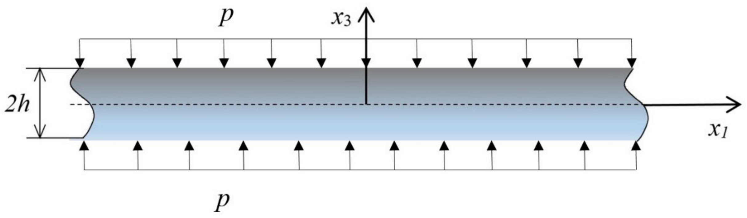
2. Statement of the Problem

Consider a linearly elastic layer with arbitrary outer contour, compressed by normal stresses p distributed along its faces, see Figure 1. The thickness of the layer 2 h is assumed to be small in comparison with a typical length scale L dictated by the variation of the prescribed loading, i.e., from the very beginning we specify the small geometric parameter
ε = h L 1 .
The equilibrium equations in the Cartesian coordinates x i   i = 1 ,   2 ,   3   a n d   x 3 h are written as
σ i j , j = 0 ,
where σ i j   i , j = 1 ,   2 ,   3 are the components of the Cauchy stress tensor.
The constitutive relations for a linear isotropic elastic solid are given by
σ i j = λ x 3 u k , k δ i j + μ x 3 u i , j + u j , i ,
where u i are the components of the displacement vector. Thus we study a transversely inhomogeneous isotropic material with the Lamé parameters λ and μ slowly varying along the thickness. Thus, the case of rapidly oscillating or decaying λ and μ (with a typical length scale much less than the thickness) is not considered in what follows.
The boundary conditions at the faces x 3 = ± h are taken in the form
σ 33 = p , u 1 = u 2 = 0 ,
where p = p x 1 , x 2 is the aforementioned normal stress. Such mixed boundary conditions are not a feature of the canonical plate and shell theories, e.g., see [23,24,25] operating with Neumann type boundary conditions expressed in terms of stresses only.
The goal of the paper is to develop an asymptotic procedure oriented to a thin inhomogeneous layer using the small parameter (1). Below we extend the previous asymptotic results for transverse compression, see [10] and references therein to the case of transverse inhomogeneity.

3. Asymptotic Solution
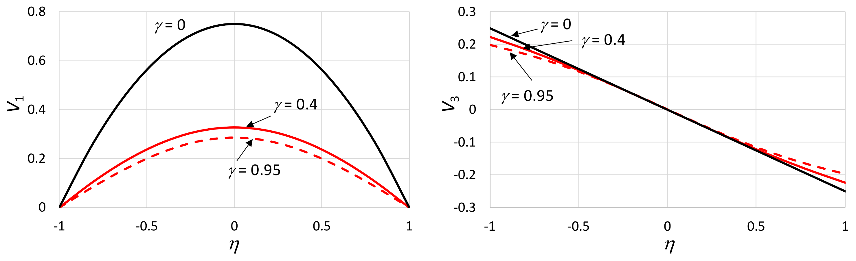
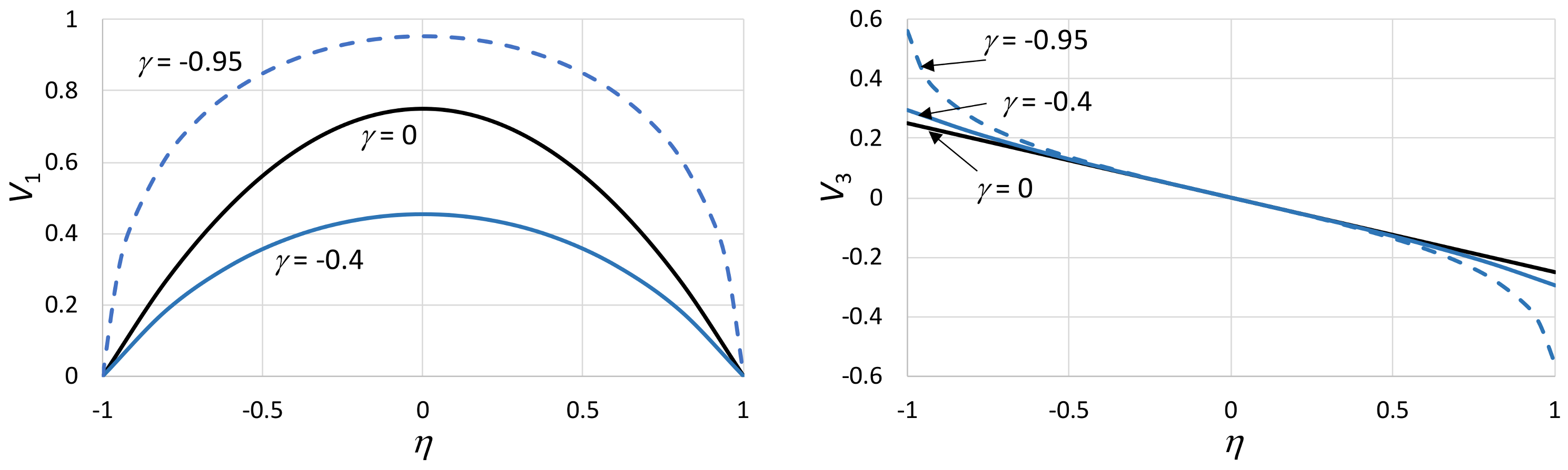
Similarly to the asymptotic derivation in [10], see also recent publications in [14,15] analysing thin transversely inhomogeneous plates and shells, we scale original variables as
ξ i = x i L ,         η = x 3 h       ( i = 1 ,   2 ) .
We also define dimensionless quantities
u i = u i h ,       u 3 = u 3 L , σ i i = ε μ 0 σ i i , σ 12 = 1 ε μ 0 σ 12 , σ 33 = ε μ 0 σ 33 ,     σ 3 i = 1 μ 0 σ 3 i , i = 1 ,   2
and
p = ε μ 0 p , λ = λ μ 0 , μ = μ μ 0 ,
where μ 0 = c o n s t is a typical value of the Lamé’s constant and all quantities with the asterisk are of the same asymptotic order.
The equilibrium equations and constitutive relations in a non-dimensional form may now be rewritten as
σ 11 ξ 1 + σ 13 η + ε 2 σ 12 ξ 2 = 0 , σ 22 ξ 2 + σ 23 η + ε 2 σ 21 ξ 1 = 0 , σ 33 η +   ε 2 σ 31 ξ 1 + σ 32 ξ 2 = 0 ,
where
σ i i = λ u 3 η + ε 2 λ u 1 ξ 1 + u 2 ξ 2 + 2 μ u i ξ i , σ 33 = ( λ + 2 μ ) u 3 η + ε 2 u 1 ξ 1 + u 2 ξ 2 , σ 12 = μ u 1 ξ 2 + u 2 ξ 1 , σ i 3 = μ u i η + u 3 ξ i , i = 1 ,   2 .
The boundary conditions modelling transverse compression become
σ 33 = p ,           u i = 0         at       η = ± 1 ,       i = 1 ,   2 .
Next, we expand the displacements and stresses in the asymptotic series in terms of the small parameter ε as
u i u 3 σ i i σ 21 σ i 3 σ 33 = u i ( 0 ) u 3 ( 0 ) σ i i ( 0 ) σ 21 ( 0 ) σ i 3 ( 0 ) σ 33 ( 0 ) + ε 2 u i ( 1 ) u 3 ( 1 ) σ i i ( 1 ) σ 21 ( 1 ) σ i 3 ( 1 ) σ 33 ( 1 ) + ,   i = 1 ,   2 .
Substituting these expansions into the Equation (8), and the boundary conditions (10) along the faces, we obtain at leading order
σ 11 ( 0 ) ξ 1 + σ 13 ( 0 ) η = 0 , σ 22 ( 0 ) ξ 2 + σ 23 ( 0 ) η = 0 , σ 33 ( 0 ) η = 0
and
σ 11 ( 0 ) = σ 22 ( 0 ) = λ u 3 ( 0 ) η , σ 33 ( 0 ) = λ + 2 μ u 3 ( 0 ) η , σ 12 ( 0 ) = μ u 1 ( 0 ) ξ 2 + u 2 ( 0 ) ξ 1 , σ 13 ( 0 ) = μ u 1 ( 0 ) η + u 3 ( 0 ) ξ 1 , σ 23 ( 0 ) = μ u 2 ( 0 ) η + u 3 ( 0 ) ξ 2
with
σ 33 0 = p ξ 1 ,   ξ 2 ,       u i ( 0 ) = 0       at       η = ± 1 ,       i = 1 ,   2 .
At next order, the governing equations and boundary conditions are given by
σ 11 ( 1 ) ξ 1 + σ 12 ( 0 ) ξ 2 + σ 13 ( 1 ) η = 0 , σ 21 ( 0 ) ξ 1 + σ 22 ( 1 ) ξ 2 + σ 23 ( 1 ) η = 0 , σ 31 ( 0 ) ξ 1 + σ 32 ( 0 ) ξ 2 + σ 33 ( 1 ) η = 0 ,
and
σ 11 ( 1 ) = λ + 2 μ u 1 0 ξ 1 + λ u 2 ( 0 ) ξ 2 + u 3 ( 1 ) η , σ 22 ( 1 ) = λ + 2 μ u 2 ( 0 ) ξ 2 + λ u 1 ( 0 ) ξ 1 + u 3 ( 1 ) η , σ 33 ( 1 ) = λ + 2 μ u 3 ( 1 ) η + λ u 1 ( 0 ) ξ 1 + u 2 ( 0 ) ξ 2 , σ 12 ( 1 ) = μ u 1 ( 1 ) ξ 2 + u 2 ( 1 ) ξ 1 , σ 13 ( 1 ) = μ u 1 ( 1 ) η + u 3 ( 1 ) ξ 1 , σ 23 ( 1 ) = μ u 2 ( 1 ) η + u 3 ( 1 ) ξ 2 .
with
σ 33 1 = 0 ,       u i ( 1 ) = 0       at       η = ± 1 ,       i = 1 ,   2 .
First, integrating Equations (12) and (13) in η we have
u i ( 0 ) = p ξ 1 ,   ξ 2 ξ i 0 η 1 μ η 1 0 η 1 λ η 2 λ η 2 + 2 μ η 2 d η 2 d η 1 + 0 η 0 η 1 1 λ η 2 + 2 μ η 2 d η 2 d η 1   + B i ξ 1 ,   ξ 2 0 η 1 μ η 1 d η 1 η A ξ 1 ,   ξ 2 ξ i + C i ξ 1 ,   ξ 2 , u 3 ( 0 ) = p ξ 1 ,   ξ 2 0 η 1 λ η 1 + 2 μ η 1 d η 1 + A ξ 1 ,   ξ 2 , σ i i 0 = λ η λ η + 2 μ η p ξ 1 ,   ξ 2 , σ 12 0 = μ η [ 2 2 p ξ 1 ,   ξ 2 ξ 2 ξ 1 0 η 1 μ η 1 0 η 1 λ η 2 λ η 2 + 2 μ η 2 d η 2 d η 1 + 0 η 0 η 1 1 λ η 2 + 2 μ η 2 d η 2 d η 1   2 η 2 A ξ 1 ,   ξ 2 ξ 2 ξ 1 + B 1 ξ 1 ,   ξ 2 ξ 2 + B 2 ξ 1 ,   ξ 2 ξ 1 0 η 1 μ η 1 d η 1 + C 1 ξ 1 ,   ξ 2 ξ 2 + C 2 ξ 1 ,   ξ 2 ξ 1 ] σ 33 0 = p ξ 1 ,   ξ 2 , σ i 3 0 = p ξ 1 ,   ξ 2 ξ i 0 η λ η 1 λ η 1 + 2 μ η 1 d η 1 + B i ξ 1 ,   ξ 2 , i = 1 ,   2 .
Then, integrating the third equation of (16) in η we have
σ 33 1 = 2 p ξ 1 ,   ξ 2 ξ 1 2 + 2 p ξ 1 ,   ξ 2 ξ 2 2 0 η 0 η 1 λ η 2 λ η 2 + 2 μ η 2 d η 2 d η 1 B 1 ξ 1 ,   ξ 2 ξ 1 + B 2 ξ 1 ,   ξ 2 ξ 2 η + D ξ 1 ,   ξ 2 .
Here we omit other formulae for first order corrections. They may be readily derived in a similar manner.
Next, applying the second boundary condition in (14) to the first equation in (18) and the first boundary condition in (17) to Equation (19) we obtain 6 linear equations for the unknown 2D functions A , B i ,   C i and D ( i = 1 ,   2 ),
p ξ 1 ,   ξ 2 I 1 ± + B ξ 1 ,   ξ 2 I 2 ± A ξ 1 ,   ξ 2 + C ξ 1 ,   ξ 2 = 0 , p ξ 1 ,   ξ 2 I 3 ± ± div B ξ 1 ,   ξ 2 D ξ 1 ,   ξ 2 = 0 ,
where B and C are the vectors with the components B i and C i , respectively, and
I 1 ± = 0 ± 1 1 μ η 1 0 η 1 λ η 2 λ η 2 + 2 μ η 2 d η 2 d η 1 + 0 ± 1 0 η 1 1 λ η 2 + 2 μ η 2 d η 2 d η 1 , I 2 ± = 0 ± 1 1 μ η 1 d η 1
and
I 3 ± = 0 ± 1 0 η 1 λ η 2 λ η 2 + 2 μ η 2 d η 2 d η 1 .
In the formulae above we define 2D differential operators specified in the plane Cartesian coordinates ξ i ,   ( i = 1 ,   2 ) , e.g.,
p ξ 1 ,   ξ 2 = 2 p ξ 1 ,   ξ 2 ξ 1 2 + 2 p ξ 1 ,   ξ 2 ξ 2 2 .
The solution of Equation (20) is given by
D ξ 1 ,   ξ 2 = 1 2 I 3 + I 3 + p ξ 1 ,   ξ 2 , div B ξ 1 ,   ξ 2 = 1 2 I 3 I 3 + p ξ 1 ,   ξ 2 C ξ 1 ,   ξ 2 = 1 2 p ξ 1 ,   ξ 2 I 1 + I 1 + + B ξ 1 ,   ξ 2 I 2 + I 2 + , A ξ 1 ,   ξ 2 = 1 2 p ξ 1 ,   ξ 2 I 1 I 1 + + B ξ 1 ,   ξ 2 I 2 I 2 + .

4. Particular Cases

Consider first the symmetric setup for which
λ η = λ η ,     μ η = μ η .
In this case we have in (21) I 1 = I 1 + , I 3 = I 3 + , I 2 = I 2 + . As a result, Formulae (23) simplify to
A ξ 1 ,   ξ 2 = 1 2 B ξ 1 ,   ξ 2 I 2 , div B ξ 1 ,   ξ 2 = 0 , C ξ 1 ,   ξ 2 = I 1 p ξ 1 ,   ξ 2 , D ξ 1 ,   ξ 2 = I 3 p ξ 1 ,   ξ 2
with
I 1 = 1 + 1 1 μ η 1 0 η 1 λ η 2 λ η 2 + 2 μ η 2 d η 2 d η 1 + 1 + 1 0 η 1 1 λ η 2 + 2 μ η 2 d η 2 d η 1 , I 2 = 1 + 1 0 η 1 1 μ η 2 d η 2 d η 1 . I 3 = 1 + 1 0 η 1 λ η 2 λ η 2 + 2 μ η 2 d η 2 d η 1 .
As next example, consider the general (asymmetric) case of plane strain deformation, for which
u 2 ( 0 ) = 0 ,       ξ 2 = 0       and       B 2 = C 2 = 0 .
Then
A ξ 1 = 1 2 p ξ 1 I 1 I 1 + + 1 2 p ξ 1 I 3 I 3 + + b ξ 1 I 2 I 2 + + a , B 1 ξ 1 = 1 2 p ξ 1 ξ 1 I 3 I 3 + + b , C 1 ξ 1 = 1 2 p ξ 1 ξ 1 I 1 + I 1 + + 1 2 p ξ 1 ξ 1 I 3 I 3 + + b I 2 + I 2 + , D ξ 1 = 1 2 2 p ξ 1 ξ 1 2 I 3 + I 3 + ,
where constants a and b may be determined from extra conditions. For example, by prohibiting vertical translation we get a = 0 . The constrain b = 0 means that there is no transverse shear stress uniform along the thickness.
Now we have for leading order non-zero displacements and stresses
u 1 ( 0 ) ξ 1 , η = p ξ 1 ξ 1 0 η 1 μ η 1 0 η 1 λ η 2 λ η 2 + 2 μ η 2 d η 2 d η 1 + 0 η 0 η 1 1 λ η 2 + 2 μ η 2 d η 2 d η 1 + 1 2 p ξ 1 ξ 1 I 3 I 3 + + b 0 η 1 μ η 1 d η 1 + 1 2 { p ξ 1 ξ 1 I 1 I 1 + + 1 2 p ξ 1 ,   ξ 2 ξ 1 I 3 I 3 + + b I 2 I 2 + } η 1 2 p ξ 1 ξ 1 I 1 + I 1 + + 1 2 p ξ 1 ξ 1 I 3 I 3 + + b I 2 I 2 + , u 3 ( 0 ) ξ 1 , η = p ξ 1 0 η 1 λ η 1 + 2 μ η 1 d η 1 1 2 p ξ 1 I 1 I 1 + + 1 2 p ξ 1 I 3 I 3 + + b ξ 1 I 2 I 2 + + a , σ i i 0 ξ 1 , η = λ η λ η + 2 μ η p ξ 1 , σ 33 0 ξ 1 ,   ξ 2 , η = p ξ 1 , σ 13 0 ξ 1 ,   ξ 2 , η = p ξ 1 ,   ξ 2 ξ i 0 η λ η 1 λ η 1 + 2 μ η 1 d η 1 + 1 2 p ξ 1 ,   ξ 2 ξ i I 3 I 3 + + b ,
Now assume in the last formulae for displacements that
λ η = Λ 1 + γ η 2 , μ η = Μ 1 + γ η 2
and p ξ 1 = P cos θ ξ 1 , where Λ , Μ , P , γ and θ are given constants with θ η 1 . Then we obtain from (28) setting, for the sake of simplicity, a = b = 0 ,
u 1 ( 0 ) ξ 1 , η = U 1 η sin θ ξ 1 , u 3 ( 0 ) ξ 1 , η = U 3 η cos θ ξ 1 ,
where
U 1 η = P 2 Λ + 2 Μ γ θ Λ Μ 1 ln 1 + γ η 2 1 + γ + 2 γ η arctan γ η arctan γ U 3 η = P γ Λ + 2 Μ arctan γ η .
Similar explicit formulae for stresses readily follow from the solution above. It can be also easily verified that the solution corresponding to displacement field (31) satisfies the boundary conditions along the faces η = ± 1 .
In the homogeneous setup ( γ = 0 ) the last formulae reduce to
U 1 η = P 2 Λ + 2 Μ θ Λ Μ + 1 1 η 2 , U 3 η = P Λ + 2 Μ η .
The last expressions agree with previous results in this area, e.g., see [10].
Numerical results are plotted in Figure 2 and Figure 3. The variation of displacements across the thickness is demonstrated for chosen values of the parameter γ characterizing the dependence of the Lamé parameters upon the transverse coordinate, see (29). For the sake of definiteness we set in the Formulae (31) Λ = 2 Μ . In these figures V 1 = U 1 Μ P θ and V 3 = U 3 Μ P . For γ > 0 (Figure 2) the studied transverse inhomogeneity has a greater effect on the tangential displacement V 1 . In this case the maximum value at γ = 0.95 is 62% less than that for the homogeneous case ( γ = 0 ). At the same time, for γ < 0 (Figure 3) the vertical displacement V 3 is more sensitive to the variation of inhomogeneity. In particular, the maximum value at γ = 0.95 is now 123% greater than that for γ = 0 .

5. Prescribed Transverse Displacements

The transverse compression can be also modelled by prescribing novel displacements along the faces of the layer. In this case, instead of the first boundary condition in (9), we have
u 3 = q ( ξ 1 ,   ξ 2 )   at   η = ± 1 ,
where q * ( ξ 1 , ξ 2 ) = q / L .
Using the zero order solution for the transverse displacement u 3 ( 0 ) in (18) together with the boundary condition (30), we arrive at the equations
u 3 ( 0 ) = p ξ 1 ,   ξ 2 0 η 1 λ η 1 + 2 μ η 1 d η 1 + A ξ 1 ,   ξ 2 , P ξ 1 ,   ξ 2 0 ± 1 1 λ η + 2 μ η d η + A ξ 1 ,   ξ 2 = q ( ξ 1 ,   ξ 2 ) ,
where P ξ 1 ,   ξ 2 is unknown function corresponding to the given stress p ξ 1 ,   ξ 2 in (18). As a result, we obtain
P ξ 1 ,   ξ 2 = 2 I 4 q ( ξ 1 ,   ξ 2 )
and
A ξ 1 ,   ξ 2 = 1 2 P ( ξ 1 ,   ξ 2 ) 0 + 1 1 λ η + 2 μ η d η + 0 1 1 λ η + 2 μ η d η ,
where I 4 = 1 + 1 1 λ * η + 2 μ * η d η .
Next, using the last formula we may restore B and C from Equation (23). Thus, we arrive at relations (18), which do not involve unknown functions anymore.

6. Concluding Remarks

Explicit asymptotic formulae are derived for transverse compression of a thin elastic layer exhibiting general inhomogeneity across the thickness. They are expressed in terms of repeated integrals. The effect of both normal stresses and displacements specified along faces is considered. For prescribed stresses arbitrary functions arising at integration through the thickness are analysed. The particular cases of a symmetric inhomogeneity and plane strain deformation are studied in detail.
Similar formulae can be obtained for other sets of boundary conditions imposed on faces, except of all given stresses. For the latter, the 2D partial differential equations governing transverse compression should generalize those for a homogeneous layer, e.g., see [26].
The established procedure can be readily extended to a thin inhomogeneous shell under transverse compression, as well as for anisotropic structures. Moreover, there is a potential of taking into account nonlinearity, due to density dependence of elastic modulus using the methodology recently developed in [27]. The underlying formulation has already proved to be useful for modelling of bones, e.g., see [28] and also fresh numerical and experimental results in [29]. Another possible extension is concerned with incorporating the stochastic nature of elastic moduli. Finally, the derived explicit formulae may be adapted to the interpretation of experimental data, not having analogues in scientific literature.

Author Contributions

Conceptualization, J.K., A.N. and A.S.M.A.; Methodology, J.K. and A.N.; Software, A.N., A.S.M.A. and B.Z.; Validation, J.K., B.Z. and A.N.; Formal analysis, J.K. and A.N.; Investigation, A.N. and A.S.M.A.; Data curation, A.N. and A.S.M.A.; Writing—original draft, J.K., A.N. and A.S.M.A.; Writing—review & editing, J.K., A.N. and B.Z.; Visualization, A.S.M.A. and B.Z. All authors have read and agreed to the published version of the manuscript.

Funding

This research has been supported in part through the project number TU-DSPP-2024-257, Taif University, Saudi Arabia.

Data Availability Statement

Dataset available on request from the authors.

Acknowledgments

Ahmed S. M. Alzaidi extends his appreciation to Taif University, Saudi Arabia, for supporting this work through project number TU-DSPP-2024-257.

Conflicts of Interest

The authors declare no conflict of interest.

References

  1. Chalhoub, M.S.; Kelly, J.M. Effect of bulk compressibility on the stiffness of cylindrical base isolation bearings. Int. J. Solids Struct. 1990, 26, 743–760. [Google Scholar] [CrossRef]
  2. Gent, A.; Lindley, P. The compression of bonded rubber blocks. Proc. Inst. Mech. Eng. 1959, 173, 111–122. [Google Scholar] [CrossRef]
  3. Koh, C.G.; Lim, H.L. Analytical solution for compression stiffness of bonded rectangular layers. Int. J. Solids Struct. 2001, 38, 445–455. [Google Scholar] [CrossRef]
  4. Pinarbasi, S.; Akyuz, U.; Mengi, Y. A new formulation for the analysis of elastic layers bonded to rigid surfaces. Int. J. Solids Struct. 2006, 43, 4271–4296. [Google Scholar] [CrossRef]
  5. Pinarbasi, S.; Mengi, Y.; Akyuz, U. Compression of solid and annular circular discs bonded to rigid surfaces. Int. J. Solids Struct. 2008, 45, 4543–4561. [Google Scholar] [CrossRef]
  6. Tsai, H.C.; Lee, C.C. Compressive stiffness of elastic layers bonded between rigid plates. Int. J. Solids Struct. 1998, 35, 3053–3069. [Google Scholar] [CrossRef]
  7. Tsai, H.C. Compression behavior of annular elastic layers bonded between rigid plates. J. Mech. 2012, 1, 1–7. [Google Scholar] [CrossRef]
  8. Brady, B.T. An exact solution to the radially end-constrained circular cylinder under triaxial loading. Int. J. Rock Mech. Min. Sci. Geomech. Abstr. 1971, 8, 165–178. [Google Scholar] [CrossRef]
  9. Qiao, S.; Lu, N. Analytical solutions for bonded elastically compressible layers. Int. J. Solids Struct. 2015, 58, 353–365. [Google Scholar] [CrossRef]
  10. Alzaidi, A.S.M.; Kaplunov, J.; Nikonov, A.; Zupančič, B. Transverse compression of a thin elastic disc. Z. Angew. Math. Phys. 2024, 75, 116. [Google Scholar] [CrossRef]
  11. Miyamoto, Y.; Kaysser, W.A.; Rabin, B.H.; Kawasaki, A.; Ford, R.G. (Eds.) Functionally Graded Materials: Design, Processing and Applications; Springer Science+Business Media: New York, NY, USA, 2013. [Google Scholar]
  12. Gupta, A.; Talha, M. Recent development in modeling and analysis of functionally graded materials and structures. Prog. Aerosp. Sci. 2015, 79, 1–14. [Google Scholar] [CrossRef]
  13. Adıyaman, G.; Öner, E.; Yaylacı, M.; Birinci, A. A study on the contact problem of a layer consisting of functionally graded material (FGM) in the presence of body force. J. Mech. Mater. Struct. 2023, 18, 125–141. [Google Scholar] [CrossRef]
  14. Ege, N.; Erbaş, B.; Kaplunov, J.; Noori, N. Low-frequency vibrations of a thin-walled functionally graded cylinder (plane strain problem). Mech. Adv. Mater. Struct. 2023, 30, 1172–1180. [Google Scholar] [CrossRef]
  15. Kaplunov, J.; Erbaş, B.; Ege, N. Asymptotic derivation of 2D dynamic equations of motion for transversely inhomogeneous elastic plates. Int. J. Eng. Sci. 2022, 178, 103723. [Google Scholar] [CrossRef]
  16. Le, K.C. An asymptotically exact first-order shear deformation theory for functionally graded plates. Int. J. Eng. Sci. 2023, 190, 103875. [Google Scholar] [CrossRef]
  17. Akhmedov, N.K.; Sofiyev, A.H. Asymptotic analysis of three-dimensional problem of elasticity theory for radially inhomogeneous transversally-isotropic thin hollow spheres. Thin-Walled Struct. 2019, 139, 232–241. [Google Scholar] [CrossRef]
  18. Huang, Q.; Gao, Y.; Hua, F.; Fu, W.; You, Q.; Gao, J.; Zhou, X. Free vibration analysis of carbon-fiber plain woven reinforced composite conical-cylindrical shell under thermal environment with general boundary conditions. Compos. Struct. 2023, 322, 117340. [Google Scholar] [CrossRef]
  19. Akhmedov, N.K.; Gasanova, N.S. Asymptotic behavior of the solution of an axisymmetric problem of elasticity theory for a sphere with variable elasticity modules. Math. Mech. Solids. 2020, 25, 2231–2251. [Google Scholar] [CrossRef]
  20. Argatov, I.; Mishuris, G. (Eds.) Contact Mechanics of Articular Cartilage Layers: Asymptotic Models; Springer: Cham, Switzerland, 2015; 335p. [Google Scholar]
  21. Goldenveizer, A.L. Algorithms for the asymptotic construction of a linear two-dimensional theory of thin shells and the Saint-Venant principle. PMM J. Appl. Math. Mech. 1994, 58, 1039–1050. [Google Scholar] [CrossRef]
  22. Gregory, R.D.; Wan, F.Y.M. On plate theories and Saint-Venant’s principle. Int. J. Solids Struct. 1985, 21, 1005–1024. [Google Scholar] [CrossRef]
  23. Aghalovyan, L.A. Asymptotic Theory of Anisotropic Plates and Shells; World Scientific: Singapore, 2015. [Google Scholar]
  24. Goldenveizer, A.L. Theory of Thin Elastic Shells; Nauka: Moscow, Russia, 1976. [Google Scholar]
  25. Goldenveizer, A.L. The general theory of elastic bodies (shells, coatings and linings). Mech. Solids 1992, 3, 3–17. [Google Scholar]
  26. Kaplunov, J.D.; Kossovich, L.J.; Nolde, E.V. Dynamics of Thin Walled Elastic Bodies; Academic Press: San Diego, CA, USA, 1998. [Google Scholar]
  27. Erbaş, B.; Kaplunov, J.; Rajagopal, K.R. Elastic bending and transverse compression of a thin plate with density-dependent Young’s modulus. Int. J. Non-Linear Mech. 2024, 160, 104651. [Google Scholar] [CrossRef]
  28. Arumugam, J.; Alagappan, P.; Bird, J.; Moreno, M.; Rajagopal, K.R. A new constitutive relation to describe the response of bones. Int. J. Non-Linear Mech. 2024, 161, 104664. [Google Scholar] [CrossRef]
  29. Abd Aziz, A.U.; Ammarullah, M.I.; Ng, B.W.; Gan, H.S.; Abdul Kadir, M.R.; Ramlee, M.H. Unilateral external fixator and its biomechanical effects in treating different types of femoral fracture: A finite element study with experimental validated model. Heliyon 2024, 10, e26660. [Google Scholar] [CrossRef]
Figure 1. Transverse compression of a thin elastic layer.
Mathematics 12 02502 g001
Figure 2. Displacement variation along the thickness of the layer for positive γ .
Mathematics 12 02502 g002
Figure 3. Displacement variation along the thickness of the layer for negative γ .
Mathematics 12 02502 g003
Disclaimer/Publisher’s Note: The statements, opinions and data contained in all publications are solely those of the individual author(s) and contributor(s) and not of MDPI and/or the editor(s). MDPI and/or the editor(s) disclaim responsibility for any injury to people or property resulting from any ideas, methods, instructions or products referred to in the content.

