Article

A Mathematical Programming Model for Minimizing Energy Consumption on a Selective Laser Melting Machine

School of Mechanical Engineering, Tongji University, Shanghai 201804, China
*
Author to whom correspondence should be addressed.
Mathematics 2024, 12(16), 2507; https://doi.org/10.3390/math12162507
Submission received: 24 July 2024 / Revised: 10 August 2024 / Accepted: 13 August 2024 / Published: 14 August 2024

Abstract

:
The scheduling problem in additive manufacturing is receiving increasing attention; however, few have considered the effect of scheduling decisions on machine energy consumption. This research focuses on the nesting and scheduling problem of a single selective laser melting (SLM) machine to reduce total energy consumption. Based on an energy consumption model, a nesting and scheduling problem is formulated, and a mixed integer linear programming model is proposed. This model simultaneously determines part-to-batch assignments, part placement in the batch, and the choice of build orientation to reduce the total energy consumption of the SLM machine. The energy-saving potential of the model is validated through numerical experiments. Additionally, the effect of the number of alternative build orientations on energy consumption is explored.

1. Introduction

Compared with conventional manufacturing, additive manufacturing (AM) has great potential to improve material efficiency, reduce lifecycle impact, and enable greater engineering capabilities [1]. Despite these advantages, AM is recognized as an energy-intensive technology, especially for large-scale parts and mass production. The formation of multiple thin layers from raw materials requires a considerable amount of energy, resulting in higher energy consumption per unit volume of material compared to conventional manufacturing techniques [2]. This aspect raises concerns about the potential negative economic and environmental impacts. Therefore, reducing energy consumption is becoming one of the most important goals driving the adoption of additive manufacturing in key industries [3].
The research of energy-aware scheduling in conventional manufacturing systems is receiving considerable attention. Various studies have considered the multi-objective scheduling problem and proposed methods to optimize the energy cost with other common scheduling criteria [4,5,6]. In these studies, the energy-saving opportunities come from a better allocation of jobs to machines with different speeds and powers, as well as a better job sequence to avoid high consumption in the periods of high electricity price.
However, few works have considered the scheduling problem that aims to reduce energy consumption in AM machines. In this research, we focus on saving the energy consumption of the selective laser melting (SLM) machine. SLM is a powder-bed-fusion AM process whereby a high-density-focused laser beam selectively scans a powder bed and those scanned and solidified layers are stacked upon each other to build a fully functional three-dimensional part, tool, or prototype [7]. SLM machines are batch processing machines that are capable of printing a group of parts at a time. According to a recent study by Lv et al. [8], the energy consumption of an SLM machine is related to the power of each subsystem and the subsystem running time. The power of each subsystem depends on the machine parameters, which are basically constant during the process. The running time of each subprocess depends on not only the process parameters (laser power, heating and cooling temperature, etc.), but also the batch parameters (total part volume, surface area, support structure volume, height, etc.). Therefore, the energy consumption can be affected by how the batches are formed. This creates an opportunity to optimize the energy of printing the parts by making better decisions such as part-to-batch assignment, nesting, and build orientation selection.
Generally, increasing the batch utilization reduces the total energy consumption. Compared to a single part, printing a full batch at a time can save more than 50% energy consumption per part [9]. To maximize the batch utilization, one needs to consider the nesting problem, which decides the part displacement and rotation around the z axis (vertical axis) and packs parts into batches. For SLM machines, no stacks are permitted because supporting structures are required for heat dissipation and fixing parts on the platform [10]. This results in a 2D nesting problem that concerns packing the projections of the parts into the build platform of the machine, which is usually a rectangle. To reduce the problem difficulty, a common way is to represent the geometry of a part with a bin. However, even for this case, the nesting problem is NP-hard [11].
On the other hand, a part generally has several optional build orientations that can satisfy the quality requirement. Changing the build orientation can lead to a variation in the part height, support structure volumes, and the projection area of the part, as shown in Figure 1. The batch height determines the number of layers and thus the total recoating time of a batch, and the volume of the support structure determines the scanning time of the support. These two factors have an impact on the energy consumption of several subsystems of the SLM machine. Therefore, the choice of the build orientation is also important for energy saving. At the same time, a proper selection of the build orientation can increase the packing efficiency and thus reduce the energy consumption.
In this study, we consider the nesting and scheduling problem that jointly handles the part-to-batch assignment, part nesting and build orientation selection on a single SLM machine to minimize the total energy consumption. The contributions of this research are as follows:
  • The energy-saving potential of nesting and scheduling decisions on a single SLM machine is studied. Based on an accurate energy consumption model, we propose a mixed-integer linear programming (MILP) model considering alternative build orientations for the nesting and scheduling problem;
  • Through numerical experiments, the performance of the proposed model is tested and validated by comparison with commercial 3D printing software. The MILP model achieves significant energy savings compared to the commercial software. The percentage of energy savings tends to increase with the number of alternative build orientations of the parts.
What remains of this paper is organized as follows. Section 2 reviews the literature. Section 3 describes the problem. Section 4 describes the energy consumption model. Section 5 proposes the mathematical model. Section 6 reports the numerical results, and Section 7 concludes the paper.

2. Literature Review

In this section, we first review the works related to the energy-aware scheduling, then we introduce some works about nesting and scheduling on AM machines, and finally we summarize the research gap.

2.1. Energy-Aware Scheduling

Many scholars have paid attention to the problem of energy-aware scheduling in manufacturing systems with conventional machines. Agrawal et al. [12] proposed three energy-aware scheduling algorithms including genetic algorithm, cellular automata and efficiency-based allocation heuristic to schedule tasks on a non-identical machines environment to minimize the makespan and energy consumption. Bruzzone et al. [13] integrated the energy-aware scheduling module with the advanced pand scheduling system to control the power peaks on the shop floor given a detailed schedule. Che et al. [14] studied the scheduling problem of unrelated parallel machines with the goal of minimizing the total power cost under a scenario that electricity prices may vary from hour to hour throughout a day. Schulz et al. [15] used a local search algorithm to solve a multi-objective problem of energy consumption, energy cost, and demand charging in a flow shop. Che et al. [16] developed a continuous-time MILP model and proposed an efficient greedy insertion heuristic to minimize the total electricity cost within a given makespan under time-of-use or time-dependent electricity tariffs. In addition, Abikarram et al. [17] addressed a parallel machine scheduling problem, in which the number of active machines and utilization are controlled to reduce the peak power.
For additive manufacturing, there are only a few related studies on energy-aware scheduling. Most studies aim to improve the energy efficiency of AM machines by optimizing the process parameters to fabricate parts with low energy consumption while meeting desired specifications. For instance, Paul et al. [18] considered the problem of finding the orientation of the part and the layer thickness that yield the minimum energy consumption for selective laser sintering (SLS). Verma et al. [19] proposed a multi-objective optimization model to find the combination of processing parameters that minimizes laser processing energy and material waste while maximizing part quality for a single SLS process. For the first time, Karimi et al. [3] proposed an MILP model that integrates process-level controls and system-level scheduling decisions. By adjusting the process parameters at different printing stages and controlling the starting time of each job, the model successfully reduces peak power and, thus, the cost of electricity tariffs for on-demand charging.

2.2. Nesting and Scheduling on AM Machines

Scheduling problems for AM machines can be categorized into three types: nesting, scheduling, nesting and scheduling [20,21]. In the past, nesting and scheduling were usually discussed separately. Recently, the number of articles focusing on the joint problem of nesting and scheduling is increasing. Chergui et al. [22] addressed the nesting and scheduling problem with the due date constraints. They proposed a heuristic approach to minimize the maximum lateness. Alicastro et al. [23] considered a nesting and scheduling problem to minimize the makespan of unrelated parallel machines. The authors proposed a local search algorithm enhanced by a reinforcement learning mechanism for neighborhood selection. In this research, the build orientations of the parts are prefixed. Li et al. [24] studied a scheduling problem in a batch processing machine with 2D capacity constraint to minimize the makespan. They proposed a greedy heuristic and a genetic algorithm to solve the problem. Che et al. [25] studied an unrelated parallel AM machine scheduling problem that requires simultaneously assigning parts to batches, orienting parts, packing parts onto a 2D platform, and assigning batches to machines to minimize the makespan. An efficient simulated annealing approach was proposed. Yu et al. [26] investigated the nesting and scheduling problem in an unrealted parallel machines environment to minimize the total tardiness of orders. They proposed different mathematical models and concluded that simplifying the complex nesting features of the problem can improve the solvability of the problem, but also lead to the potential packing infeasibility of batches. Zipfel et al. [27] considered the scenario where sequence-dependent setups are required between batches of different material. They proposed an iterated local search metaheuristic to minimize the total weighted tardiness of orders. Recently, Nascimento [28] proposed an exact solution approach based on Bender’s decomposition framework and constrain programming to solve the nesting and scheduling of parts with complex shapes.

2.3. Research Gap

Many studies have focused on reducing the energy consumption and costs by scheduling or adjusting the machine on–off state. But few have paid attention to the energy-saving benefit brought by nesting and scheduling decisions in AM machines.
Baumers et al. [29] compared the energy consumption of a build with a single part to that of multiple parts, and the full-build utilization produced a large (97.79%) energy saving on the EOSINT P 390 printer. They also showed that printing a single part in different build orientations consumes different amounts of energy. Furthermore, Piili et al. [30] found that a full build can reach a cost reduction of 81–92% compared to single part build, and the nesting solution is the major variable that users can influence the energy in a multi-part fabrication environment. Both studies reveal the potential of energy saving in AM machines by a proper nesting and scheduling, but a solution to obtain the optimal nesting and scheduling decisions is not provided.
On the other hand, although the nesting and scheduling problem has been investigated in several studies, none have considered the objective of energy savings except for our conference paper [31], which emphasizes the trade-off between productivity and energy consumption in multiple machines.
In summary, our work is driven by the exploration of energy-saving potential in SLM machines through optimized nesting and scheduling decisions. The primary objective is to formulate the nesting and scheduling problem as a mathematical programming model. By solving this model, one can determine the optimal part-to-batch assignments, part nesting configurations, and build orientation selections when printing a set of parts on a single SLM machine.

3. Problem Description

Consider a set of parts J = { 1 , , n } to be printed on a single SLM machine. Each part j J has a given volume v j and surface s j and a set of optional build orientations K j . Each build orientation k K j corresponds to a 3D geometry with four parameters { h j k , l j k , w j k , s j k } , which are the height, length, and width of the rectangle projection, and the volume of the supporting structure, respectively. The SLM machine can process a batch of parts at a time. The capacity of the machine is represented by a cuboid of length L W , width W W , and height H W . A group of parts can be placed on the same batch if their projections do not overlap and their geometries are within the platform boundaries. Parts must be placed parallel to the length or width of the platform and can be rotated by 90° around the Z axis. The goal is to decide the build orientation for each part, place and schedule them on the machines to minimize the total energy consumption.
We impose the following assumptions:
  • For any part j J , any optional build orientation k K j can satisfy the quality requirement of the part j.
  • Each part is represented by its minimum bounding box, and thus, the projection of any part is a rectangle on the build platform.
  • There is a minimum distance requirement between any parts placed on the build platform. Without loss of generality, it is assumed that this distance has been included in the size of each part.
  • The process parameters (e.g., laser power, layer thickness, hatching distance) are identical for all parts.
  • The power of each subsystem of the SLM machine is assumed to be constant during a subprocess.

4. Energy Consumption Model

Energy forecasting is the key for the evaluation and reduction in SLM energy consumption. Energy consumption models for AM can be divided into three categories: specific energy models [32], stage-based energy models [9], and subsystem-based energy models [33].
Models that compute the energy demand by multiplying the specific energy consumption (SEC) and the weight or volume of a part are called specific energy models. Here, the SEC refers to the energy consumed for each deposited kilogram or volume of material. It may be affected by the utilization of the build volume, build density, and orientation, and hence, different values were reported in the literature for the same AM technology [33,34]. To describe the energy consumption in a more reasonable way, substage-based energy consumption models were proposed. These models predict the total energy consumption by summing the energy consumed in each stage. The power and time of each operation stage are obtained through measurement, and thus, these models can only be applied on the specific AM machine. Subsystem-based models work in a similar way, they estimate the total energy by summing the energy consumed by each machine subsystem. In this research stream, most works focus on the energy modeling of the machine subsystem [18], while the operating status of different subsystems at different stages are ignored.
Recently, Lv et al. [8] proposed a more accurate energy consumption model that jointly considers the power of the machine subsystem, the time of the subprocess, and the working state of the machine subsystem in each subprocess. In this paper, we adopt this model and combine it with the mathematical programming model for energy optimization.

4.1. Energy Consumption Calculation

Typically, an SLM machine consists of eight subsystems, and the process of printing a batch can be divided into four subprocesses, as shown in Figure 2. The energy consumption of the SLM machine for printing a single batch is calculated as:
E = f = 1 F E f = f = 1 F l = 1 L p f t l k f l = P K T ,
where E f is the energy consumption of the f-th subsystem, p f is the power of the f-th subsystem, t l is the time of the l-th subprocess, and k f l [ 0 , 1 ] is a factor describing the working state of the f-th subsystem in the l-th subprocess. In the following subsections, we describe the way to calculate the processing time of subprocesses, the power of subsystems, and the state of each subsystem in each subprocess.

4.2. Processing Time of Subprocesses

A typical SLM process includes four subprocesses: heating, laser exposure, recoating, and cooling. During the heating phase, the following relationship holds:
t h = C 1 T 2 + C 2 T C 3 ,
where t h represents the time spent in the heating stage, T represents the temperature of the platform at a certain moment. The parameters C 1 , C 2 , and C 3 are machine-dependent factors and are obtained by regression using the experimental data. See Lv et al. [8] for more technical details. Thus, the time of the heating phase is expressed as:
Δ t h = t h ( T f ) t h ( T i ) ,
where T i is the initial temperature of the platform, and T f is the final temperature after heating.
The construction stage is the main production process, including powder recoating and laser exposure. The total time spent in this phase is expressed as:
t b = t l + t r ,
where t l is the laser exposure time and t r is the powder spreading time. The time of the sub-stages of the laser exposure process is expressed as:
t l = t b + t c + t p + t s = j B s j n l v b Δ y + j B s j n l v c Δ y + j B V j v p + j B s j k v s ,
where t b , t c , t p , t s are the laser exposure time to scan the border, fill contour, hatch volume, and build supports, s j is the area of the outer and inner surfaces of part j scanned as boundaries during construction [ mm 2 ], B is the set of parts in the batch, n l is the number of lasers operating during manufacturing, v b and v c are the speeds for scanning the boundaries and filling contours [mm/s], respectively; Δ y is the layer thickness [mm], V j and s j k are the volumes of the part and support [ mm 3 ], respectively; v p ˙ and v s ˙ are the build-up rate for the part and supports [ mm 3 /s], both can be expressed as:
v ˙ = n l × D × Δ y × v ,
where D is the hatching distance [mm/s], v is the scanning speed for part or support. The recoating time can be expressed as:
t r = N t r 0 ,
where t r 0 is the time required for spreading a layer of powder. The number of slices depends on the height of the batch and the layer thickness, which can be expressed as:
N = H Δ y .
After the last layer has been scanned, the platform is gradually cooled down in the inert gas used to prevent the oxidation of the metal powder. The following relationship holds:
t c = C 4 T 2 C 5 T + C 6 ,
where T is the temperature of the platform at a certain moment, and the constants C 4 , C 5 , and C 6 are obtained by regression from the experimental data. Hence, the time of the cooling phase is expressed as:
Δ t c = t c ( T c ) t c ( T b ) ,
where T b is the temperature of the platform before cooling and T c is the final temperature.

4.3. Power of Subsystems

The power parameters of each subsystem are summarized in Table 1. The values of each parameter are machine-dependent and can be measured by the power acquisition device, including data acquisition chassis, data acquisition card, voltage sensor, current sensor, etc. For details, please refer to Lv et al. [8]. Note that the power of the laser subsystem could be different during the scanning of the border, filling contour, hatching volume, and building supports; for convenience, we treat the laser used in these subprocesses as four different subsystems, and thus the total energy consumption can be obtained by Equation (1).

4.4. State of Subsystems

Generally, a subsystem of an SLM machine can be fully on, off, or running intermittently in different subprocesses. For example, the platform heater is fully on during the preheating phase to raise the temperature of the platform to the required level, while during the laser exposure phase, it runs intermittently to keep the temperature constant. Therefore, to correctly estimate the energy consumption of each subsystem, it is critical to identify their actual operating states during each subprocess.
To this end, the working state factor k f l is introduced. For the f-th subsystem, k f l is the ratio of the actual running time to the total time of the l-th subprocess. As shown in Figure 2, the basic subsystem and water circulation unit are running all the time, whilst the laser, powder spreading motor, electric valve, and gas circulation pump motor only operate at certain stages. In these cases, the k f l is either 1 or 0. The platform heater and water cooling unit operate intermittently. To decide the values of k f l for these two subsystems, measurements are often required. See Lv et al. [8] for details of the measurement procedure.

5. Mathematical Programming Model

In this section, we propose an MILP model for the defined problem and several means to improve the model efficiency. After, we introduce some improvements upon the model.

5.1. MILP Model

The MILP model is given as follows. The sets are as follows:
  • J: set of parts.
  • F = { bs , ht , wc , co , lsb , lfc , lvh , lss , rm , ev , gp } : set of subsystems. bs is the basic system, ht is the heater, wc is the water circulation system, co is the water cooling unit, lsb is the laser unit for scanning border, lfc is the laser unit for filling contour, lvh is the laser unit for volume hatching, lss is the laser unit for scanning supporting structure, rm is the recoater motor, ev stands for the electric values, gp is the gas circulation pump motor.
  • L = { ph , sb , fc , vh , ss , rc , co } : set of subprocesses. ph is the preheating, sb is the scanning border, fc is the filling contour, vh is volume hatching, ss is the building of support structure, rc is the recoating, co is the cooling.
  • K j : set of alternative build orientations of part j.
  • B: set of available batches on machine.
The parameters are as follows:
  • v j : volume of part j.
  • a j : surface area of part j.
  • D: the minimum allowed distance from the parts to the platform boundary.
  • d: the minimum allowed distance between parts.
  • t r 0 : recoating speed of machine.
  • L W , W W , H W : length, width, and height of the build platform.
  • h j k , l j k , w j k , s j k : height, length, width, and supporting structure volume of the k-th orientation of part j.
  • n l : number of lasers.
  • v b : speed for scanning border.
  • v c : speed for filling contour.
  • v p ˙ : build-up rate for the part.
  • v s ˙ : build-up rate for the support.
  • Δ y : layer thickness.
  • p f : power of the subsystem f.
  • T P H : the time spent in the preheating subprocess.
  • T C O : the time spent in the cooling subprocess.
  • ϕ f l : the power coefficient of the subsystem f in the subprocess l, ϕ f l = 0 means that the subsystem f is not active in the subprocess l, ϕ f l = 1 means that the subsystem f is fully active during the subprocess l; ϕ f l ( 0 , 1 ) means that the subsystem f is intermittently running during the subprocess l, that is, ϕ f l = P f l * P f where P f l * represents the measured power of subsystem f in subprocess l.
The decision variables are as follows:
  • X j b : equals 1 if part j is assigned to the b-th batch, 0 otherwise;
  • Y j b : equals 1 if part j selects the k-th optional build orientation, 0 otherwise;
  • ( x j , y j ) : coordinates of the left-bottom point of part j’s projection on the platform;
  • O j : equals 1 if part j is placed such that its length is parallel to that of the platform.
The auxiliary variables are as follows:
  • Z b : equals 1 if the b-th batch on machine is formed, 0 otherwise;
  • P L j j : equals 1 if part j’s right–top point is placed to the left of part j’s left–bottom point in the same batch, 0 otherwise;
  • P B j j : equals 1 if part j’s right–top point is placed below part j’s left–bottom point in the same batch, 0 otherwise;
  • H b : height of the b-th batch;
  • E b : the energy consumption of the b-th batch;
  • T l b : the processing time of the subprocess l in the b-th batch;
  • M: a large number.
In the model, the decision variables P L j j , P B j j , P L j j , P B j j together describe the positional relationship of parts j and j .
The nesting and scheduling problem of a single SLM machine is formulated as:
min b B E b ,
j J X j b M Z b , b B ,
b B X j b = 1 , j J ,
k K j Y j k = 1 , j J ,
j J a j X j b n l v b Δ y T s b , b , b B ,
j J a j X j b n l v c Δ y T f c , b , b B ,
j J v j X j b v p ˙ T v h , b , b B ,
j J X j b k K j s j k Y j k v s ˙ T s s , b , b B ,
T p h , b = T P H , b B ,
T c o , b = T C O , b B ,
H b k K j Y j k h j k M ( 1 X j b ) , b B , j J ,
t r 0 H b Δ y T r c , b , b B ,
E b f F l L p f ϕ f l T l b , b B ,
H b H W , b B ,
x j + k K j Y j k l j k L W + M ( 1 O j ) , j J ,
x j + k K j Y j k w j k L W + M O j , j J ,
y j + k K j Y j k w j k W W + M ( 1 O j ) , j J ,
y j + k K j Y j k l j k W W + M O j , j J ,
x j + k K j Y j k l j k + d x j + M ( 1 P L j j ) + M ( 1 O j ) , j , j J ,
x j + k K j Y j k w j k + d x j + M ( 1 P L j j ) + M O j , j , j J ,
y j + k K j Y j k w j k + d x j + M ( 1 P B j j ) + M ( 1 O j ) , j , j J ,
y j + k K j Y j k l j k + d x j + M ( 1 P B j j ) + M O j , j , j J ,
P L j j + P B j j + P L j j + P B j j X j b + X j b 1 , j , j J , j < j , b B ,
Z b { 0 , 1 } , b B ,
T l b 0 , l L , b B ,
X j b { 0 , 1 } , j J , b B ,
Y j k { 0 , 1 } , j J , k K j ,
H b 0 , b B ,
P L j j , P B j j { 0 , 1 } , j , j J ,
x j , y j 0 , j J ,
O j { 0 , 1 } , j J ,
Constraints (12) ensure that the batches cannot be assigned without forming. Constraints (13) specify to assign parts to only one batch. Constraints (14) guarantee that the part selects only one build orientation. Constraints (15) calculate the time for the laser to scan the border. Constraints (16) calculate the time for the laser to fill contour. Constraints (17) calculate the time for the laser to hatch the volume. Constraints (18) calculate the time for the laser to build the support structure. Constraints (19) define the preheating time. Constraints (20) define the cooling time. Constraints (21) define the batch height. Constraints (22) calculate the powder recoating time. Constraints (23) calculate the energy consumption of the batch. Constraints (24) guarantee that the height of the batch is less than the height of the machine. Constraints (25)–(28) ensure that parts do not exceed the machine boundary. Constraints (29)–(32) ensure that when parts are assigned to the same batch, they will not overlap. Specifically, when P L j j equals 1, part j is placed on the left side of part j , so the right edge of part j does not exceed the left edge of part j . When P L j j equals 0, this constraint is released. Constraints (31) and (32) express the same relationship in the vertical direction. Constraints (33) guarantee that when part j and part j are assigned to the same batch, i.e., X j b , X j b equal to 1, part j and j choose at least one of the positional relationships. For example, when P L j j equals 1, P B j j equals 0, P L j j equals 0 and P B j j equals 0, part j is on the left semi-axis of part j. When P L j j equals 1, P B j j equals 1, P L j j equals 0, and P B j j equals 0, part j is located in the third quadrant of part j. Another positional relationship can be obtained by setting different values of P L j j and P B j j .

5.2. Model Improvements

We improve the model as follows. First, the following constraints are introduced to break the symmetry of batches:
Z ( b 1 ) Z b , b B .
Second, to linearize (18), we introduce an auxiliary variable e j b to represent the support structure volume of part j in the b-th batch, and replace Constraints (18) with the following:
e j b k K j Y j k s j k M ( 1 X j b ) , j J , b B ,
j J e j b v s T s s , b , b B .
Finally, in order to further improve the solution efficiency of the model, we define the upper bound of the big-M values in different constraints, as reported in Table 2.

5.3. Model Parameter: The Number of Available Batches

Besides the big-M values, another critical parameter influencing model efficiency is the number of available batches on the machine, i.e., how many batches can be opened on the machine. Let n B denote the cardinality of B. A large n B results in a substantial number of decision variables X j i b , which may complicate the resolution process. Conversely, a small n B may lead to suboptimal solutions when n B is smaller than the number of batches required in the optimal solution. In the worst case, the model could become infeasible if n B is set below the minimum number of batches necessary to accommodate all parts. Thus, determining an appropriate value for n B is crucial.
Let n B fea represent the minimum number of batches required to ensure model feasibility, and let n B opt denote the number of batches in the optimal solution. It is evident that
n B fea n B opt | J | ,
where | J | is the number of parts to be printed. However, n B fea and n B opt are unknown and difficult to determine precisely. To address this, we propose a simple trial-and-error approach as follows:
Step 1:
Set label is unnecessary and can be removed. Answer: Confirmed, we have removed the bold. n B = η | J | , where η ( 0 , 1 ) ;
Step 2:
Solve the MILP model with the current value of n B ;
Step 3:
If the model is infeasible or if the obtained solution includes n B opened batches, then increment n B by 1 and return to Step 2. Otherwise, proceed to the next step;
Step 4:
Terminate and output the results.

6. Numerical Results
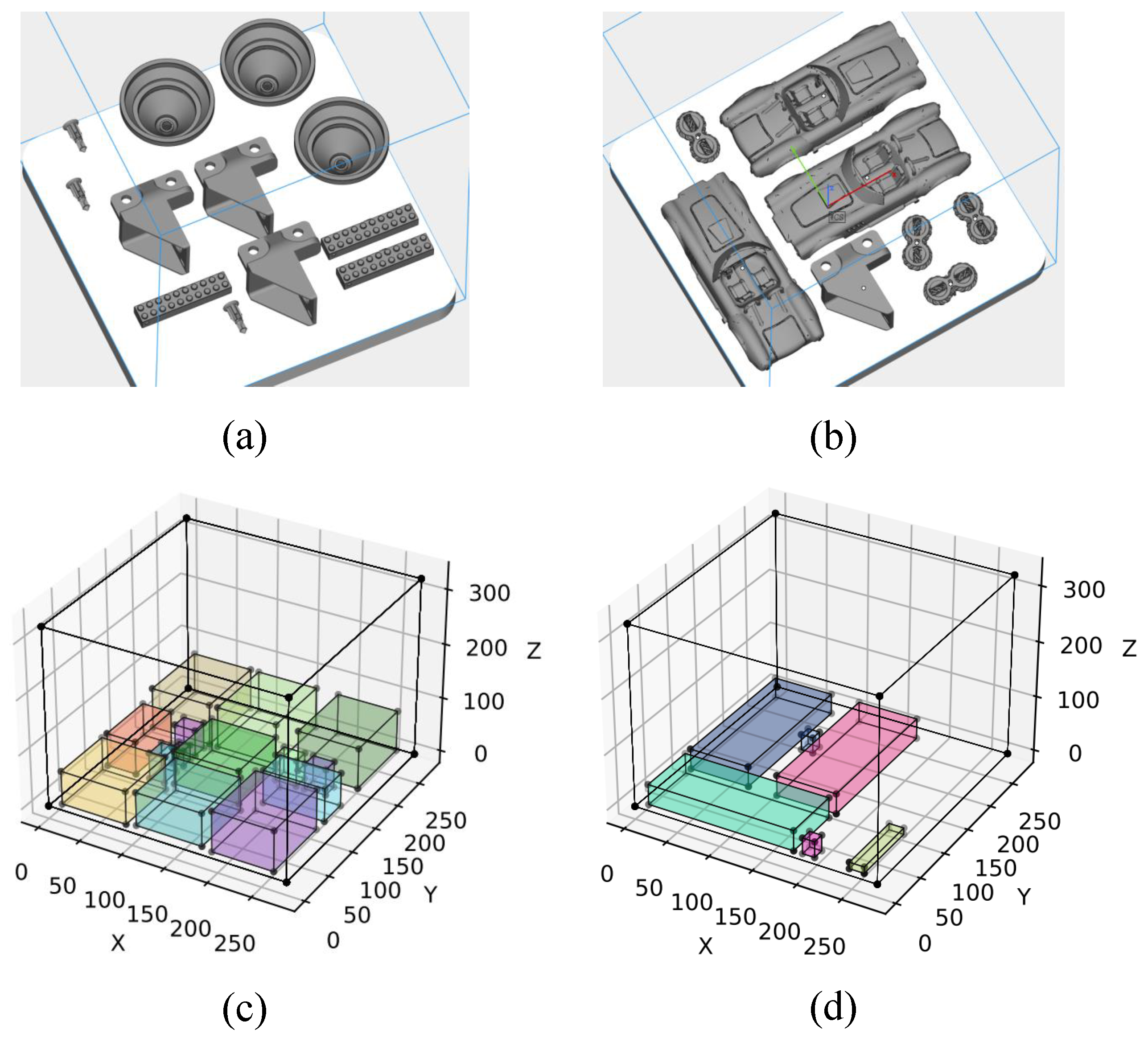
6.1. Test Instance

The part models are downloaded from the website https://www.stlfinder.com/3dmodels/free-3d-models/ (accessed on 13 August 2024). All the part information such as volume, surface, support structure, and height are obtained from the STL files using a commercial 3D printing software named Materialise Magics. Details of the parts are provided in Appendix A.

6.2. Machine and Process Parameters

The parts are to be fabricated using aluminum AlSi10Mg powder on an SLM280HL machine. The machine is equipped with two 400 W fiber lasers with a laser beam diameter of 80 µm. The length, width, and height of the build platform of the machine is 268 mm, 268 mm, and 315 mm, respectively. The power of machine subsystems and the power coefficients of the subsystems in different subprocesses are summarized in Table 3.
The parts are to be fabricated in an inert gas atmosphere. Before the construction process began, the oxygen content will be reduced from 21% to below 0.1% to prevent the oxidation and reaction of the AlSi10Mg powder. The platform will be heated from 27 °C to 150 °C to relieve thermally induced internal stress of the fabricated part, which results in a preheating time of Δ t c = t c ( 80   ° C ) t c ( 150   ° C ) . During the manufacturing process, two lasers work together. The time required for spreading a layer of powder is 11 s. After building the parts, the platform will be cooled from 150 °C to 80 °C, which leads to a cooling time of Δ t c = t c ( 80   ° C ) t c ( 150   ° C ) . The process parameters of the SLM machine are given in Table 4.

6.3. Experiment Setup

With the above settings, we conducted two experiments:
  • Experiment 1: The first numerical experiment compares the energy consumption of printing a set of 20 parts when MILP and Magics are applied for the nesting and scheduling. Magics uses the default build orientation for each part, which corresponds to the smallest Z axis height. For MILP, we assume that each part has five different alternative build orientations, which are provided by the Magics software according to different rules. The MILP model is solved by the Gurobi solver (ver 9.5.2) with a maximum CPU runtime of 7200 s.
  • Experiment 2: A design of experiments is performed with the following factors and levels: number of parts—{20, 25, 30}, number of alternative build orientations—{1, 3, 5, 7}. This results in 12 experiments. We analyze the impact of the number of parts and alternative build orientations on the energy consumption of the MILP model.

6.4. Results Analysis
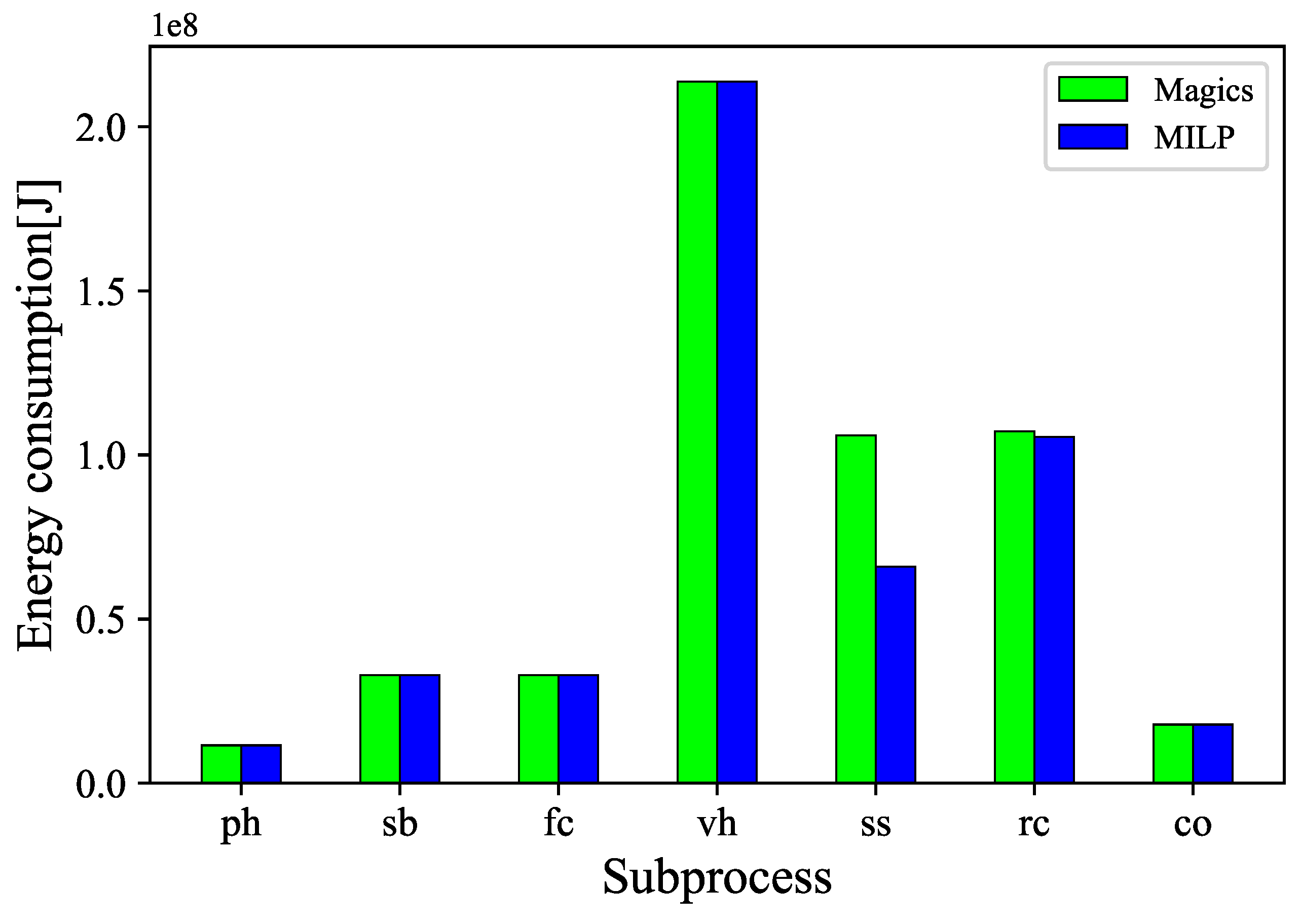
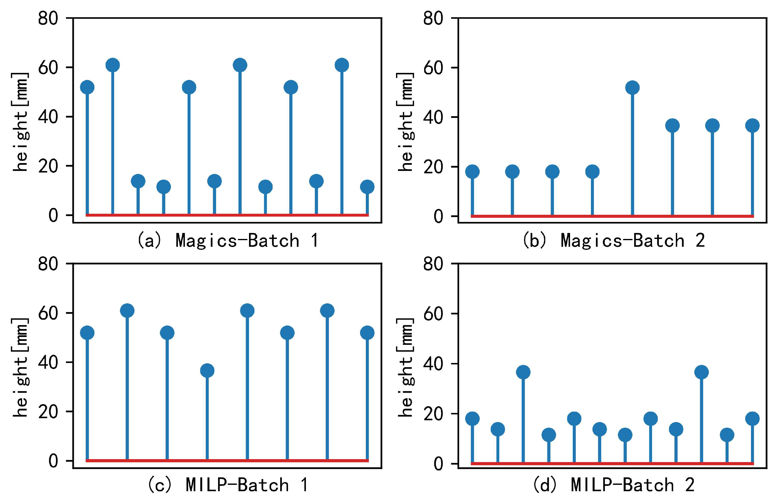
6.4.1. Experiment 1

The batch placements of the Magics and MILP are illustrated in Figure 3. In addition, we also summarize the batch information, printing time, and energy consumption of the two approaches in Table 5. Compared to Magics, the MILP model reduces the energy consumption by 41.67 MJ (8.62%). Furthermore, the total processing time of MILP is less than that of Magics. Indeed, the energy consumption of the machine is determined by both the time of each subprocess and the power of each subsystem. In the case of constant energy power, the reduction in energy consumption can only be achieved by reducing the running time of subprocesses.
Table 6 presents the energy savings associated with different subsystems. The “Percentage” column indicates the proportion of energy savings contributed by each subsystem, calculated as follows:
E f ( MILP ) E f ( Magic ) Total energy saving × 100 ,
where E f ( MILP ) is the total energy consumed by subsystem f in the MILP solution, and E f ( Magics ) is that of the Magics solution. This table shows that the laser for the support structure provides the greatest energy savings, followed by the water circulation unit, water cooling unit, basic subsystem, and platform heater. In contrast, the recoater motor, electric valves, and gas circulation pump contribute relatively little to energy savings. This is because the MILP solution, which involves less subprocess time, leads to more energy savings in subsystems with a higher power consumption. Thus, reductions in the subprocess time have a greater impact on energy-intensive units, explaining why the support structure construction shows significant energy savings when there is a notable difference in the time required for building the support structure in the solutions of MILP and Magics. Similarly, Table 7 presents the energy savings associated with different subprocesses. As shown, the majority of energy savings is achieved during the support structure building subprocess, with the remainder obtained during the recoating phase.
To investigate the reasons behind energy savings and time reductions, we compare the two solutions obtained by Magics and MILP in terms of time differences across different subprocesses (Figure 4), energy consumption across different subprocesses (Figure 5), and energy consumption for different subsystems (Figure 6). As illustrated in Figure 4, the primary differences between the two solutions are observed in the time required to build the support structure and the time needed to spread the powder. According to Formulas (2)–(10), for the same printer and process parameters, heating and cooling times are fixed. Additionally, when the part volume and surface area are identical, the times for scanning the border, filling contour, and volume hatching remain constant. The time required to print the support structure is dependent on its volume, while the powder recoating time is influenced by the number of slices. Table 5 shows that variations in the support structure volume and the number of slices between the two solutions account for the differences in processing time. Furthermore, Figure 2 reveals that nearly all subsystems are active during both the laser exposure and recoating stages. Since the laser system and recoater motor operate alternately during these stages, changes in the time required to build the support structure and recoating time significantly impact the energy consumption of most subsystems. This explains the observed reductions in energy consumption.
Overall, the primary factors contributing to energy savings are the reductions in time during the recoating phase and the construction of the support structure. Consequently, the printing efficiency improves while optimizing energy consumption. For a nesting problem, the choice of the part build orientation significantly impacts both the processing time and energy consumption of the batch. This is because the build orientation affects the support structure, the height of the part, and the projection area of the part, which in turn influences batch utilization.

6.4.2. Experiment 2

The results of instances with different a number of parts and build orientations are summarized in Table 8, where ins_20_1 represents the instance having 20 parts and each part has only one build orientation 1, ins_20_3 represents the instance with 20 parts and each has three different build orientations, etc. The column “EC” represents the total energy consumption, the column “EV” represents the energy consumption per unit volume, and the column “ES” represents the proportion of energy-saving of MILP compared to Magics. Specifically, the energy consumption of Magics when printing 20 parts, 25 parts, and 30 parts is 522.25 MJ, 663.79 MJ, and 883.27 MJ, respectively. The column “Gap” is the optimality gap of the best feasible solution. The Column “B” represents the number of batches opened in the solution. All the EC values are obtained from the MILP model.
It can be observed from Table 8 that even when all parts share a single build orientation, consistent with Magics’ build direction, MILP can still achieve some energy savings. In this scenario, the volume, surface area, and support structure volume of all parts remain identical in both solutions; the only variation lies in part-to-batch allocation, specifically in how the parts are grouped into batches. Figure 7 illustrates the differences in part height within the batches provided by Magics and MILP in instance ins_20_1. In Batch 1 of both solutions, the batch height (maximum part height within the batch) is the same at 60.9 mm. However, in Batch 2, the batch height in Magics is 51.9 mm, whereas MILP results in a lower batch height of 36.6 mm. This indicates that, even with the same number of parts and build orientations, different scheduling results can lead to varying total batch heights and, consequently, different energy consumption.
Additionally, when the number of printed parts remains the same, increasing the build orientations of the parts can also reduce the energy consumption. For example, with 20 parts, as the number of build orientations increases from 1 to 7, the energy consumption per unit volume of parts gradually decreases, and the energy savings achieved by MILP are also greater. It is understandable that increasing the number of build orientations for a part can reduce energy consumption. Different build orientations result in varying support structure volumes and part heights. By choosing a build orientation with a smaller support structure volume without increasing the batch height, energy consumption can be significantly reduced. Furthermore, as the number of parts increases, the advantage of the MILP model over Magics becomes more pronounced. For instance, when the number of printed parts increases from 20 to 25, as seen in instances ins_20_5 and ins_25_5, the percentage of energy savings rises significantly. This trend is also observed in other instances, where increased numbers of printed parts with the same build orientation result in greater energy savings compared to Magics scheduling.
To summarize, the following observations can be obtained from Table 8:
  • Increasing the build orientation of parts can reduce energy consumption to some extent, but it also complicates the model and increases the optimality gap.
  • Increasing the number of printed parts can lead to reduced energy consumption compared to Magics, but it also makes the model more challenging to solve.

7. Conclusions

In this study, we address the nesting and scheduling problem on a single SLM machine with the goal of reducing our energy consumption. We consider the 2D nesting subproblem involved in packing parts into batches and account for the multiple optional build orientations for each part. We propose a mathematical programming model and several enhancements to strengthen it.
By comparing the results from solving the MILP model with those provided by commercial 3D printing software, we demonstrate the potential for energy savings through optimized nesting and scheduling. The energy savings range from 3.46% to 15.63% across various instances, depending on the number of parts and build orientations. Specifically, when the build orientation of parts is fixed, the MILP model reduces the total height of batches by optimizing the distribution of parts among batches. This reduces the total number of layers and, consequently, the overall energy consumption. When multiple build orientations are available, the MILP model achieves even greater energy savings due to the added flexibility in optimization. However, this increased flexibility also raises the complexity of solving the model, necessitating a careful trade-off.
The numerical results indicate that there is still potential for further energy savings through improvements in model efficiency. Future work will focus on developing efficient solution approaches, such as matheuristics and metaheuristics, to handle large-scale problems. Additionally, this study addresses the nesting and scheduling problem on a single SLM machine. However, since multi-machine environments better reflect industrial practices, extending the research to such environments will also be considered. This extension would require accounting for various factors, including different additive manufacturing technologies, build platform sizes, and the powder materials used by the machines on the shop floor.

Author Contributions

Conceptualization, C.Y.; methodology, C.Y.; software, J.L.; validation, C.Y. and J.L.; formal analysis, C.Y.; investigation, J.L.; resources, C.Y.; data curation, J.L.; writing—original draft preparation, J.L.; writing—review and editing, C.Y.; visualization, J.L.; supervision, C.Y.; project administration, C.Y.; funding acquisition, C.Y. All authors have read and agreed to the published version of the manuscript.

Funding

This research was funded by National Natural Science Foundation of China (72301196), and Tongji University “Fundamental Research Funds for the Central Universities”.

Data Availability Statement

The raw data supporting the conclusions of this article and the source codes will be made available by the authors upon request.

Conflicts of Interest

The authors declare no conflict of interest.

Appendix A. Part Information

The information of each part type is given in Table A1. Each part can have maximum optional build orientations which are provided by the Materialise Magics software according to different rules. We used in total six different part types to generate the instances. For example, ins_20_5 contains four copies of part 1 and part 2, and three copies of part 3 to part 6. Each part has five optional build orientations 1–5.
Table A1. Part parameters.
Part TypeBuild OrientationVolume [ mm 3 ]Surface Area [ mm 2 ] Supporting Structure Volume [ mm 3 ]Length [mm]Width [mm]Heigth [mm]
116744.008607.801724.0057.5024.6018.00
26744.008607.802596.0038.8024.5041.70
36744.008607.802174.0022.1032.0046.00
46744.008607.801489.0018.0024.5047.60
56744.008607.802667.0042.1028.1036.50
66744.008607.802162.0040.3824.7239.98
76744.008607.802545.0040.3827.7440.05
2137,635.0017,532.0023,352.0073.0064.0051.90
237,635.0017,532.0014,668.0078.3072.7076.40
337,635.0017,532.003396.0087.7070.5074.40
437,635.0017,532.0015,453.0073.0074.0064.00
537,635.0017,532.0013,779.0069.0056.9076.70
637,635.0017,532.003694.0073.1785.9074.03
737,635.0017,532.002025.0073.1762.4978.14
311029.001017.0098.0028.3013.8013.80
21029.001017.00142.0024.9013.8025.10
31029.001017.00376.0021.8015.9026.90
41029.001017.000.0013.7013.8028.30
51029.001017.00536.0026.7014.9022.40
61029.001017.00155.0024.8713.7524.87
71029.001017.00138.5519.7721.9525.14
41105,909.0045,458.3036,239.0069.00169.0036.60
2105,909.0045,458.3010,143.0075.70165.70101.00
3105,909.0045,458.3034,743.00139.0093.20155.70
4105,909.0045,458.3044,612.0069.8036.60169.00
5105,909.0045,458.3047,096.0090.60147.40136.20
6105,909.0045,458.3013,352.0085.35158.36122.65
7105,909.0045,458.3020,212.00141.1090.55157.22
5128,588.1020,398.801183.0077.0077.0060.90
228,588.1020,398.805542.0077.0077.0060.90
328,588.1020,398.8025,217.0076.7060.9076.70
428,588.1020,398.8025,150.0069.7074.6076.70
528,588.1020,398.8012,042.0073.2074.1071.10
628,589.1020,398.8025,145.0072.4573.7376.90
728,589.1020,398.8025,145.0074.0272.4776.74
616310.009792.003908.0016.6079.7011.50
26310.009792.003726.0034.7071.2060.60
36310.009792.005187.0027.2037.2080.40
46310.009792.002425.0016.6011.5079.70
56310.009792.003737.0029.6073.2057.40
66310.009792.002439.0030.7816.1781.23
76310.009792.003267.0026.3662.5765.43

References

  1. Huang, R.; Riddle, M.; Graziano, D.; Warren, J.; Das, S.; Nimbalkar, S.; Cresko, J.; Masanet, E. Energy and emissions saving potential of additive manufacturing: The case of lightweight aircraft components. J. Clean. Prod. 2016, 135, 1559–1570. [Google Scholar] [CrossRef]
  2. Yoon, H.; Lee, J.; Kim, H.; Kim, M.; Kim, E.; Shin, Y.; Chu, W.; Ahn, S. A comparison of energy consumption in bulk forming, subtractive, and additive processes: Review and case study. Int. J. Precis. Eng. Manuf.-Green Technol. 2014, 1, 261–279. [Google Scholar] [CrossRef]
  3. Karimi, S.; Kwon, S.; Ning, F. Energy-aware production scheduling for additive manufacturing. J. Clean. Prod. 2021, 278, 123183. [Google Scholar] [CrossRef]
  4. Jia, Z.; Zhang, Y.; Leung, J.; Li, K. Bi-criteria ant colony optimization algorithm for minimizing makespan and energy consumption on parallel batch machines. Appl. Soft Comput. 2017, 55, 226–237. [Google Scholar] [CrossRef]
  5. Zhou, S.; Li, X.; Du, N.; Pang, Y.; Chen, H. A multi-objective differential evolution algorithm for parallel batch processing machine scheduling considering electricity consumption cost. Comput. Oper. Res. 2018, 96, 55–68. [Google Scholar] [CrossRef]
  6. Wang, S.; Wang, X.; Yu, J.; Ma, S.; Liu, M. Bi-objective identical parallel machine scheduling to minimize total energy consumption and makespan. J. Clean. Prod. 2018, 193, 424–440. [Google Scholar] [CrossRef]
  7. Kruth, J.P.; Vandenbroucke, B.; Van Vaerenbergh, J.; Mercelis, P. Benchmarking of different SLS/SLM processes as rapid manufacturing techniques. In Proceedings of the International Conference Polymers & Moulds Innovations PMI, Gent, Belgium, 20–23 April 2005. [Google Scholar]
  8. Lv, J.; Peng, T.; Zhang, Y.; Wang, Y. A novel method to forecast energy consumption of selective laser melting processes. Int. J. Prod. Res. 2021, 59, 2375–2391. [Google Scholar] [CrossRef]
  9. Faludi, J.; Baumers, M.; Maskery, I.; Hague, R. Environmental impacts of selective laser melting: Do printer, powder, or power dominate? J. Ind. Ecol. 2017, 21, S144–S156. [Google Scholar] [CrossRef]
  10. Zhang, J.; Yao, X.; Li, Y. Improved evolutionary algorithm for parallel batch processing machine scheduling in additive manufacturing. Int. J. Prod. Res. 2020, 58, 2263–2282. [Google Scholar] [CrossRef]
  11. Lodi, A.; Martello, S.; Vigo, D. Recent advances on two-dimensional bin packing problems. Discret. Appl. Math. 2002, 123, 379–396. [Google Scholar] [CrossRef]
  12. Agrawal, P.; Rao, S. Energy-aware scheduling of distributed systems. IEEE Trans. Autom. Sci. Eng. 2014, 11, 1163–1175. [Google Scholar] [CrossRef]
  13. Bruzzone, A.; Anghinolfi, D.; Paolucci, M.; Tonelli, F. Energy-aware scheduling for improving manufacturing process sustainability: A mathematical model for flexible flow shops. CIRP Ann. 2012, 61, 459–462. [Google Scholar] [CrossRef]
  14. Che, A.; Zhang, S.; Wu, X. Energy-conscious unrelated parallel machine scheduling under time-of-use electricity tariffs. J. Clean. Prod. 2017, 156, 688–697. [Google Scholar] [CrossRef]
  15. Schulz, S.; Neufeld, J.; Buscher, U. A multi-objective iterated local search algorithm for comprehensive energy-aware hybrid flow shop scheduling. J. Clean. Prod. 2019, 224, 421–434. [Google Scholar] [CrossRef]
  16. Che, A.; Zeng, Y.; Lyu, K. An efficient greedy insertion heuristic for energy-conscious single machine scheduling problem under time-of-use electricity tariffs. J. Clean. Prod. 2016, 129, 565–577. [Google Scholar] [CrossRef]
  17. Abikarram, J.; McConky, K.; Proano, R. Energy cost minimization for unrelated parallel machine scheduling under real time and demand charge pricing. J. Clean. Prod. 2019, 208, 232–242. [Google Scholar] [CrossRef]
  18. Paul, R.; Anand, S. Process energy analysis and optimization in selective laser sintering. J. Manuf. Syst. 2012, 31, 429–437. [Google Scholar] [CrossRef]
  19. Verma, A.; Rai, R. Sustainability-induced dual-level optimization of additive manufacturing process. Int. J. Adv. Manuf. Technol. 2017, 88, 1945–1959. [Google Scholar] [CrossRef]
  20. Oh, Y.; Witherell, P.; Lu, Y.; Sprock, T. Nesting and scheduling problems for additive manufacturing: A taxonomy and review. Addit. Manuf. 2020, 36, 101492. [Google Scholar] [CrossRef]
  21. Pinto, M.; Silva, C.; Thürer, M.; Moniz, S. Nesting and scheduling optimization of additive manufacturing systems: Mapping the territory. Comput. Oper. Res. 2024, 165, 106592. [Google Scholar] [CrossRef]
  22. Chergui, A.; Hadj-Hamou, K.; Vignat, F. Production scheduling and nesting in additive manufacturing. Comput. Ind. Eng. 2018, 126, 292–301. [Google Scholar] [CrossRef]
  23. Alicastro, M.; Ferone, D.; Festa, P.; Fugaro, S.; Pastore, T. A reinforcement learning iterated local search for makespan minimization in additive manufacturing machine scheduling problems. Comput. Oper. Res. 2021, 131, 105272. [Google Scholar] [CrossRef]
  24. Li, X.; Zhang, K. Single batch processing machine scheduling with two-dimensional bin packing constraints. Int. J. Prod. Econ. 2018, 196, 113–121. [Google Scholar] [CrossRef]
  25. Che, Y.; Hu, K.; Zhang, Z.; Lim, A. Machine scheduling with orientation selection and two-dimensional packing for additive manufacturing. Comput. Oper. Res. 2021, 130, 105245. [Google Scholar] [CrossRef]
  26. Yu, C.; Matta, A.; Semeraro, Q.; Lin, J. Mathematical models for minimizing total tardiness on parallel additive manufacturing machines. IFAC-PapersOnLine 2022, 55, 1521–1526. [Google Scholar] [CrossRef]
  27. Zipfel, B.; Neufeld, J.; Buscher, U. An iterated local search for customer order scheduling in additive manufacturing. Int. J. Prod. Res. 2024, 62, 605–625. [Google Scholar] [CrossRef]
  28. Nascimento, P.J.; Silva, C.; Antunes, C.H.; Moniz, S. Optimal decomposition approach for solving large nesting and scheduling problems of additive manufacturing systems. Eur. J. Oper. Res. 2024, 317, 92–110. [Google Scholar] [CrossRef]
  29. Baumers, M.; Tuck, C.; Wildman, R.; Ashcroft, I.; Hague, R. Energy inputs to additive manufacturing: Does capacity utilization matter? In Proceedings of the International Solid Freeform Fabrication Symposium, Austin, TX, USA, 8–10 August 2011; University of Texas at Austin: Austin, TX, USA, 2011. [Google Scholar]
  30. Piili, H.; Happonen, A.; Väistö, T.; Venkataramanan, V.; Partanen, J.; Salminen, A. Cost estimation of laser additive manufacturing of stainless steel. Phys. Procedia 2015, 78, 388–396. [Google Scholar] [CrossRef]
  31. Lin, J.; Yu, C.; Lu, J. A bi-objective optimization method to minimize the makespan and energy consumption on parallel SLM machines. In Proceedings of the 2023 IEEE 19th International Conference on Automation Science and Engineering (CASE), Auckland, New Zealand, 26–30 August 2023; IEEE: Piscataway, NJ, USA, 2023; pp. 1–6. [Google Scholar]
  32. Kellens, K.; Baumers, M.; Gutowski, T.G.; Flanagan, W.; Lifset, R.; Duflou, J.R. Environmental dimensions of additive manufacturing: Mapping application domains and their environmental implications. J. Ind. Ecol. 2017, 21, S49–S68. [Google Scholar] [CrossRef]
  33. Yi, L.; Krenkel, N.; Aurich, J.C. An energy model of machine tools for selective laser melting. Procedia CIRP 2018, 78, 67–72. [Google Scholar] [CrossRef]
  34. Ingarao, G.; Priarone, P.; Deng, Y.; Paraskevas, D. Environmental modelling of aluminium based components manufacturing routes: Additive manufacturing versus machining versus forming. J. Clean. Prod. 2018, 176, 261–275. [Google Scholar] [CrossRef]
Figure 1. A batch of parts with different build orientations.
Mathematics 12 02507 g001
Figure 2. Working status of different machine subsystems during the SLM process. The dark color, light color, and blank areas represent the subsystems running all the time, intermittently, and out of service.
Mathematics 12 02507 g002
Figure 3. The placement for the scheduling by MILP and Magics on ec_20-5: (a) Magics Batch 1; (b) Magics Batch 2; (c) MILP Batch 1; and (d) MILP Batch 2.
Mathematics 12 02507 g003
Figure 4. The duration of different subprocesses. Ph is preheating, sb is scan border, vh is volume hatching, ss is support structure, rc is powder spreading, and co is cooling.
Mathematics 12 02507 g004
Figure 5. The energy consumption of different subprocesses. Ph is preheating, sb is scan border, vh is volume hatching, ss is support structure, rc is powder spreading, and co is cooling.
Mathematics 12 02507 g005
Figure 6. The energy consumption of different subsystems. bs is basic subsystem, ht is platform heater, wc is water circulation unit, co is water cooling unit, lsb is laser for scanning border, lfc is laser for filling contour, lvh is laser for volume hatching, lss is laser for support structure, rm is Recoater, ev is electric valves, and gp is gas circulation pump motor.
Mathematics 12 02507 g006
Figure 7. Height distribution of parts across different batches for two scheduling solutions from instance ins_20_1.
Mathematics 12 02507 g007
Table 1. Power of the different subsystems.
SubsystemPower [W]
Basic subsystem P b s
Platform heater P h t
Water circulation unit P w c
Water-cooling unit P c o
Laser-scanning border P l s b
Laser-filling contour P l f c
Laser volume hatching P l v h
Laser support structure P l s s
Recoater motor P r c
Electric valves P e v
Gas circulation pump motor P g p
Table 2. Big-M values for different constraints.
ConstraintsBig-M Value
(12) M = | J |
(21) M = max j J , k K j h j k
(25) (28) M = max j J , k K j l j k
(26) (27) M = max j J , k K j w j k
(29) M = max j J , k K j l j k + L W
(30) M = max j J , k K j w j k + L W
(31) M = max j J , k K j w j k + W W
(32) M = max j J , k K j l j k + W W
(43) M = max j J , k K j s j k
Table 3. The power and power coefficient of the different subsystems.
SubsystemPower [W]Pre HeatingScan BorderFill ContourVolume HatchingSupport StructureRe CoatingCooling
Basic subsystem 569.7 1111111
Platform heater 1122.3 1 0.4826 0.4826 0.4826 0.4826 0.4826 0
Water circulation unit 713.3 1111111
Water-cooling unit 1739.4 0.168 0.353 0.353 0.353 0.353 0.353 0.216
Laser-scanning border 1770.9 0100000
Laser-filling contour 1770.9 0010000
Laser volume hatching 2022.9 0001000
Laser support structure 2022.9 0000100
Recoater motor 52.1 0000010
Electric valves 32.1 1111110
Gas circulation pump motor 69.1 0111110
Table 4. Process parameters.
Process ParameterScan BorderFill ContourVolume HatchingSupport Structure
Power of the laser [W]300300350350
Scanning speed [mm/s]73073016501000
Layer thickness [mm]0.030.030.030.03
Hatching distance [mm]--0.130.13
Table 5. Comparison of the results of two methods.
ParametersMagicsMILP
Batch 1 Batch 2 Total Batch 1 Batch 2 Total
Surface area [ mm 2 ] 220,689382,340603,029276,929326,100603,029
Part volume [ mm 3 ] 146,217188,334334,551186,356148,195334,551
Support volume [ mm 3 ] 108,969141,951250,92043,618112,625156,243
Number of slices203117293760248112203701
Utilization rate47.63%57.84%52.7%63.72%47.70%55.7%
Number of parts1282014620
Makespan [s]63,74977,965141,71468,85163,448132,299
Total energy consumption [MJ]225.66296.59522.25241.84238.72480.56
Table 6. The energy saving contribution of different subsystems.
Machine SubsystemEnergy Saving [MJ]Percentage [%]
1-Basic subsystem5.3612.86
2-Platform heater5.112.24
3-Water circulation unit6.7216.13
4-Water cooling unit5.7813.87
5-Laser for support structure17.7342.55
6-Recoater motor0.030.07
7-Electric valves0.30.72
8-Gas circulation pump motor0.651.56
Total energy saving41.67100
Table 7. The energy saving contribution of different subprocess.
Machine SubprocessEnergy Saving [MJ]Percentage [%]
1-Preheating00
2-Scan border00
3-Fill contour00
4-Volumne hatching00
5-Support structure40.0095.99
6-Recoating1.674.01
7-Cooling00
Total energy saving41.67100
Table 8. Energy consumption with different numbers of parts and build orientations.
InstanceEC [MJ]EV [J/ mm 3 ]ES [%]Gap [%]B
ins_20_1507.73841.973.460.002
ins_20_3481.06797.748.535.172
ins_20_5480.56796.918.625.342
ins_20_7479.91795.838.756.462
ins_25_1625.23839.385.817.663
ins_25_3602.57808.969.225.323
ins_25_5577.11774.7813.061.582
ins_25_7570.31765.6514.081.592
ins_30_1782.87840.8111.377.403
ins_30_3746.03801.2515.5412.293
ins_30_5745.24800.4015.6315.763
ins_30_7769.41826.3612.8920.213
Disclaimer/Publisher’s Note: The statements, opinions and data contained in all publications are solely those of the individual author(s) and contributor(s) and not of MDPI and/or the editor(s). MDPI and/or the editor(s) disclaim responsibility for any injury to people or property resulting from any ideas, methods, instructions or products referred to in the content.

